Two-Layer Conditional Prediction of Soil Electrical Conductivity Assisted by Post-Irrigation Soil Moisture Trajectories in Farmland of the Bachu Irrigation District

Abstract

Using multi-depth continuous observations from nine farmland sites in the Bachu irrigation district, Xinjiang (November 2024–April 2026), this study developed a two-layer conditional prediction model to test whether predicted soil-moisture trajectories improve apparent electrical conductivity (EC) prediction beyond a persistence benchmark. Four prediction windows (0–1, 1–3, 3–7, and 7–15 d) were evaluated using time-forward validation under observed ERA5 forcing, paired ablation, SHAP, and post-hoc meteorological-deficit linkage analysis. For EC₂₀, the R² values were 0.978, 0.923, 0.727, and −1.376, with corresponding Skill values of −0.001, 0.277, 0.540, and 0.635; absolute performance at 7–15 d remained unreliable. EC₄₀ achieved R² of 0.943–0.987, with Skill of 0.029–0.325, and EC₆₀ achieved R² of 0.737–0.974, with Skill of 0.065–0.177. Ablation showed the clearest gain for EC₂₀ at 3–7 d (ΔR² = 0.193; ΔSkill = 0.325), whereas most other combinations showed no consistent improvement. At 0–1 d, SHAP contributions of predicted moisture trajectories to EC₂₀, EC₄₀, and EC₆₀ were 39.2%, 37.6%, and 26.8%, respectively. Meteorological-deficit linkage responses varied by depth and horizon but were generally limited. Overall, trajectory benefits were depth- and horizon-dependent and reflected model dependence rather than causal water–salt mechanisms. The framework is currently applicable mainly to monitored, unfrozen post-irrigation periods without additional wetting recharge.

1. Introduction

Soil salinization remains a long-standing challenge to sustainable, high-quality agricultural production in arid irrigation districts. Owing to limited precipitation, intense evaporation, and frequent irrigation inputs, soil water and salts continuously undergo infiltration, leaching, evaporative concentration, and redistribution within the soil profile [1]. In irrigated farmland, salinity dynamics are not an isolated soil chemical process but are closely coupled with water supply, soil temperature, evapotranspiration conditions, and irrigation processes [2]. Particularly in arid regions, the increase in soil water content shortly after irrigation may promote salt dilution and downward transport [3], whereas during irrigation intervals, intensified evapotranspiration and root-zone water depletion may lead to renewed salt accumulation in the topsoil [4]. Therefore, assessment of farmland salinity risk should not focus solely on salinity at a single time point, but should also consider post-irrigation water redistribution, soil evaporative water loss, and salt transport and reaccumulation associated with water movement [5].

Agricultural production in Xinjiang and other arid regions of northwestern China is highly dependent on irrigation. Water-saving practices such as mulched drip irrigation improve water-use efficiency but also alter soil water and salt transport processes [6]. Compared with conventional flood irrigation, drip irrigation delivers water more locally, resulting in more pronounced water–salt differences between wetted and non-wetted zones [7], while evaporation, crop water uptake, and salt redistribution during irrigation intervals become more complex [8]. Previous studies have mainly examined farmland water–salt balance from the perspectives of irrigation quota, irrigation interval, leaching fraction, and yield response, providing a basis for optimizing water-saving irrigation regimes [9]. However, practical farmland water–salt management still requires a clearer understanding of the dynamic evolution of soil moisture and EC responses over different post-irrigation time windows, including whether root-zone moisture continues to decline after irrigation ceases [10] and whether salinity in the cultivated layer is at risk of reaccumulation [11]. Freeze–thaw processes are also an important stage of soil water–heat–salt dynamics in arid farmland [12]. During freezing, surface cooling and ice formation alter the direction of profile water movement, causing water and associated salts to redistribute toward the freezing zone [13]. After thawing, enhanced evaporation from shallow soil may again promote salt accumulation near the surface [14]. Studies in southern Xinjiang and other arid regions have shown that winter irrigation, mulching practices, and freeze–thaw processes can all affect soil temperature, water storage, and salt leaching, and that soil water content, temperature, and electrical conductivity are closely related [15]. These findings indicate that farmland salinity dynamics exhibit distinct stage-dependent characteristics, and that growing-season irrigation and evapotranspiration, together with winter freeze–thaw and salt reaccumulation processes, should be examined within an integrated water–heat–salt framework [16].

Current approaches to soil salinity research mainly include field sampling, remote sensing inversion, and numerical simulation [17]. Field sampling provides relatively direct measurements but lacks temporal continuity, making it difficult to capture changes in soil moisture and salt reaccumulation occurring within hours to days after irrigation [18]. Remote sensing is suitable for regional-scale salinity monitoring and enables rapid characterization of spatial salinity patterns, but provides limited information on water–salt dynamics within the root zone and deeper soil profile [19]. Process-based physical models can describe water and salt transport processes, but generally require relatively complete soil hydraulic parameters, irrigation boundary conditions, solute transport parameters, and initial conditions, which may constrain their application to long-term continuous monitoring and multi-site farmland studies [20]. Therefore, developing models that combine predictive capability with process interpretability on the basis of existing observations represents a feasible direction for farmland water–heat–salt research.

In recent years, in situ sensors and continuous monitoring technologies have provided higher-temporal-resolution data for investigating soil water–heat–salt processes [21]. Continuous monitoring at multiple depths can simultaneously capture variations in soil EC, water content, and temperature, facilitating identification of soil responses to irrigation, rainfall, enhanced evapotranspiration, and freeze–thaw transitions [22]. Several studies have combined continuous monitoring data with machine-learning models to predict soil moisture and salinity [23]. In this context, a two-layer sequential modeling strategy is particularly informative: soil moisture is first predicted using environmental and hydrometeorological information, and the predicted moisture is subsequently incorporated as an important input to the salinity model, thereby representing the influence of soil water dynamics on salinity changes. For farmland in arid irrigation districts, this concept can be further extended into a two-layer prediction framework linking meteorological deficit, moisture trajectory, and depth-specific EC response.

However, existing studies have focused more on regional salinity inversion, water–salt status estimation in wetlands, or water–salt balance under specific irrigation scenarios, whereas short-term prediction of water–salt responses during inter-irrigation periods in farmland remains relatively limited [24]. For practical farmland water–salt management, it is still necessary to determine whether root-zone moisture will continue to decline over the following days in the absence of additional irrigation, whether evapotranspiration deficits will intensify, and whether EC at different soil depths will exhibit risks of reaccumulation or redistribution [25]. Directly predicting future EC using only current EC, current moisture, and meteorological variables may largely treat EC dynamics as a continuation of the initial state, while overlooking the effects of post-irrigation water redistribution, soil temperature variation, profile gradients, and stage-dependent processes on EC responses. Therefore, a two-layer conditional prediction model capable of representing the transmission of water–heat process information should be developed using continuous monitoring data [26].

In this study, we developed a physical-baseline-assisted two-layer residual-corrected conditional prediction model for soil moisture and apparent EC, rather than a single direct EC prediction model. In the first layer, a physical baseline for soil moisture was constructed using the initial moisture state, historical response features, meteorological deficit over the prediction window, interlayer moisture gradients, and lagged responses in deeper layers. Machine learning was then used to learn the residuals between the physical baseline and observations, thereby predicting future soil moisture at depths of 20, 40, and 60 cm. The first-layer predicted moisture, moisture changes relative to initialization, and interlayer moisture gradients jointly characterize the post-irrigation moisture trajectory. In the second layer, the out-of-fold moisture predictions from the first layer, apparent EC at initialization, empirical EC–moisture interaction terms, and relevant process features were incorporated into the EC physical baseline, followed by further residual correction to obtain predictions of EC₂₀, EC₄₀, and EC₆₀. This structure was designed to test whether predicted moisture trajectories provide incremental information for apparent EC prediction beyond a persistence benchmark based on the current state, without interpreting model-explanation results as direct causal evidence of specific water–salt transport mechanisms.

Accordingly, multi-depth continuous monitoring data from nine farmland sites in the Bachu irrigation district were used to conduct two-layer conditional prediction of soil EC assisted by post-irrigation moisture trajectories. Soil moisture, temperature, and apparent EC at the end of an irrigation or significant wetting event were used as initialization conditions, and moisture and apparent EC at depths of 20, 40, and 60 cm were sequentially predicted over four prediction windows: 0–1 d, 1–3 d, 3–7 d, and 7–15 d. Because the model used point-specific matched ERA5 meteorological data that had already been realized between initialization and the target time, the present evaluation represents retrospective conditional prediction under observed meteorological forcing, rather than operational forecasting under unknown future weather conditions. We hypothesized that: (1) predicted post-irrigation moisture trajectories provide incremental information for apparent EC prediction beyond the persistence benchmark; and (2) the contribution of moisture trajectories and overall model performance vary with soil depth and prediction horizon. The main objectives were to: (1) characterize intra-annual variation and profile differentiation of apparent EC in farmland within the study area; (2) develop and evaluate a two-layer conditional prediction model for soil moisture and EC under post-irrigation conditions without additional irrigation or significant wetting recharge; and (3) evaluate model dependence on different features and local statistical associations using SHapley Additive exPlanations (SHAP) and post-hoc scenario linkage analysis of meteorological deficit.

2. Materials and Methods

2.1. Study Area Description

The study area is located in the Bachu County irrigation district, Kashgar Prefecture, Xinjiang, within the oasis agricultural region along the lower reaches of the Yarkand River. The region is characterized by low precipitation and strong evaporation, and farmland water supply depends primarily on irrigation. Consequently, soil moisture dynamics are closely associated with field management practices [27]. Under the combined effects of arid climatic conditions and irrigated agriculture, soil EC varies in response to irrigation recharge, evaporative water loss, and profile water redistribution, exhibiting distinct intra-annual stages and vertical differentiation among soil depths [28].

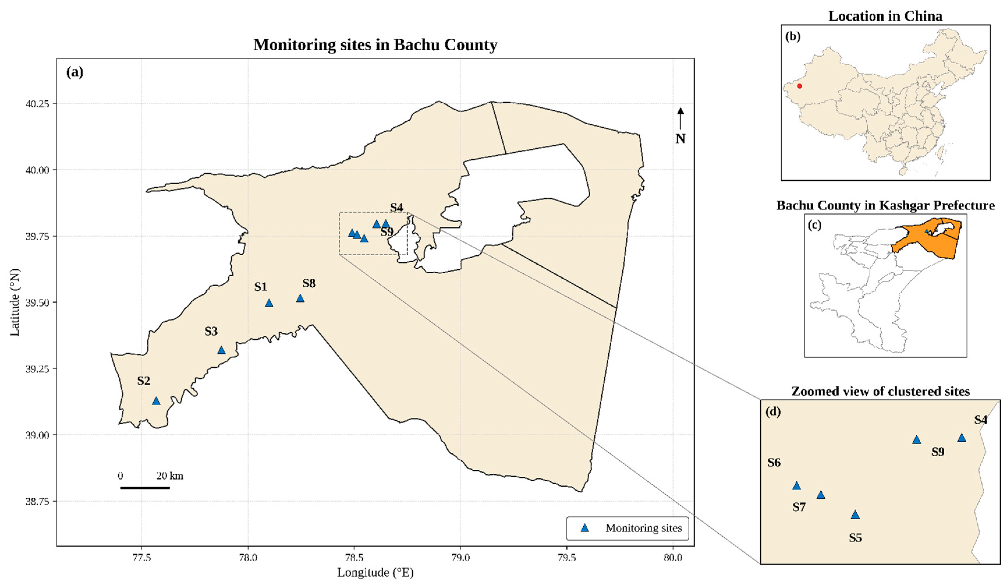
Cotton is the dominant crop in the study area, and field management includes winter irrigation, spring irrigation, and irrigation during the growing season. Because irrigation recharge, evapotranspiration, and changes in soil-profile moisture occur alternately throughout the year, the responses of EC to moisture variation may differ between the cultivated layer and deeper soil layers. To investigate the continuous intra-annual variation in farmland soil EC and its relationships with soil moisture and temperature in the Bachu irrigation district, nine continuous soil-monitoring sites were selected as the primary study sites and designated S1–S9. The monitoring sites were generally distributed along the agricultural area of the lower Yarkand River irrigation district. Site selection considered similarities in farmland distribution, cropping systems, and irrigation management, while also accounting for practical constraints including equipment security, power supply and communication conditions, interference from field management, and permission for installation from local authorities and farmers. The spatial distribution of the monitoring sites is shown in Figure 1.

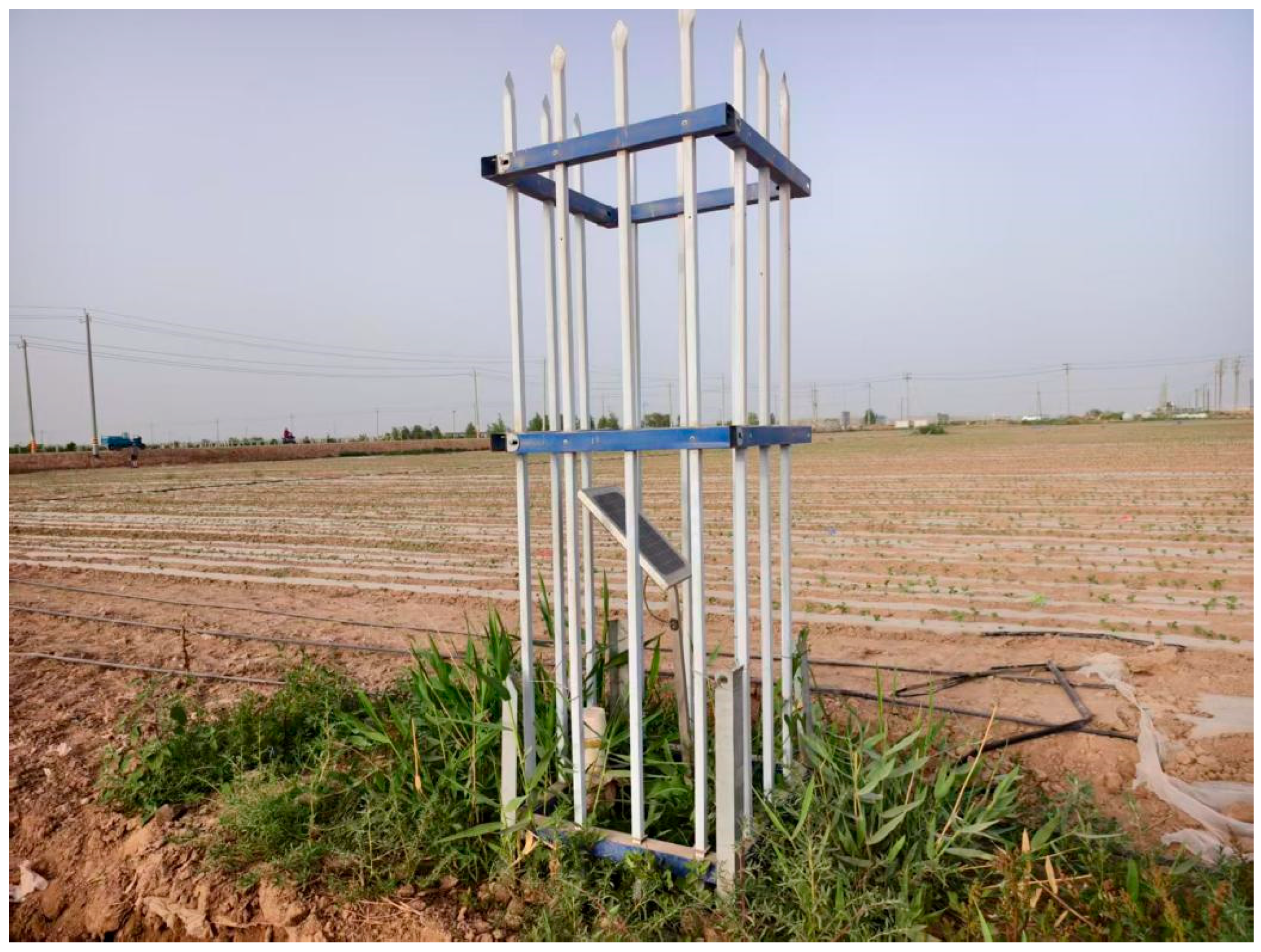
At each monitoring site, a Zhisang ETY150 tubular continuous monitoring station for soil water, salinity, and temperature, manufactured by Dongfang Zhigan (Zhejiang) Technology Co., Ltd. (Hangzhou, China), was installed to simultaneously record volumetric soil water content, soil temperature, and apparent electrical conductivity at multiple depths. Volumetric soil water content was determined based on the dielectric response of the soil, apparent electrical conductivity was measured using an alternating-current conductance method, and soil temperature was measured using a temperature-sensitive element. The general specifications of the ETY series include a soil water-content measurement range from dry to saturated soil with an accuracy of ±2%, a temperature range of −25 to 80 °C with an accuracy of ±0.5 °C, and a salinity measurement range of approximately 0–17 dS/m, with an accuracy of ±10% below 5 dS/m; measurements at higher salinity levels require calibration. The built-in temperature sensor is mainly used to compensate for the effects of temperature on soil moisture measurements. In this study, the apparent electrical conductivity measured in situ by the sensors is uniformly denoted as EC. The monitoring equipment and its field installation are shown in Figure 2.

During equipment installation, the soil profile at each monitoring site was surveyed by depth, and soil texture was recorded for the 0–20, 20–40, 40–60, 60–100, and 100–150 cm layers. The spatial and vertical variations in soil texture among the monitoring sites are presented in

Table 1. Soil texture types at different soil depths across the nine monitoring sites.

Site ID	0–20 cm	20–40 cm	40–60 cm	60–100 cm	100–150 cm
S1	Sand	Sand	Sand	Sand	Sand
S2	Loam	Loam	Loam	Clay	Loam
S3	Silt loam	Silt loam	Silt loam	Silt loam	Silt loam
S4	Clay loam	Clay loam	Clay loam	Clay loam	Clay loam
S5	Silt loam	Silt loam	Silt loam	Sand	Clay
S6	Loam	Loam	Silt loam	Silt loam	Clay
S7	Loam	Loam	Clay	Clay	Clay
S8	Heavy loam *	Heavy loam *	Heavy loam *	Heavy loam *	Clay
S9	Sandy loam	Sandy loam	Sandy loam	Sandy loam	Clay

Note: * Heavy loam is a local soil-texture designation retained from the original field survey records and does not correspond to a standard USDA or WRB texture class. Because the available data are insufficient for reliable conversion to a standard texture category, the original survey term is retained and its non-standard classification status is explicitly noted.

. The available soil data in this study were primarily used to characterize soil texture at different depths. Because complete information on diagnostic horizons, diagnostic properties, and diagnostic materials required by the World Reference Base for Soil Resources (WRB) was unavailable, WRB soil classification was not performed for the monitoring sites.

2.2. Data Preprocessing and Dataset Construction

This study used multi-depth measurements of soil volumetric water content, soil temperature, and apparent electrical conductivity from nine continuous soil-monitoring sites. The monitoring period extended from November 2024 to April 2026, with an original temporal resolution of 2 h and measurement depths of 10, 20, 40, 60, 80, 100, 120, and 150 cm. Data from November 2024 to October 2025 were used to characterize intra-annual variations in soil EC and their hydrothermal background, whereas valid post-irrigation samples with no additional irrigation and unfrozen soil were used to construct the physical-baseline-assisted two-layer residual-corrected conditional prediction model for soil moisture and EC.

The raw monitoring data were first organized by monitoring-site ID, timestamp, and soil depth to generate a dataset containing timestamp, site ID, soil depth, volumetric soil water content, soil temperature, and EC. Duplicate records for the same site, time, and depth were then removed, and data continuity and completeness were examined chronologically.

Meteorological data were obtained from the hourly ERA5-Seamless reanalysis dataset and matched point-by-point to each monitoring site according to its geographic coordinates. The variables included air temperature, relative humidity, wind speed, solar radiation, precipitation, and reference evapotranspiration demand. After spatial matching and temporal alignment, the meteorological data were linked to the soil-monitoring records using the actual timestamps and were used to construct meteorological forcing and water-deficit indicators from the forecast initialization time to the target time. Precipitation was treated as a natural meteorological forcing in the model but was not directly used to identify irrigation-recharge events.

Meteorological variables within each prediction window were derived from ERA5-Seamless reanalysis data that had already been realized. Therefore, the present evaluation represents retrospective conditional prediction under known meteorological forcing rather than operational forecasting under unknown future weather conditions.

The EC values reported by the sensors were used to represent apparent soil electrical conductivity under continuous in situ monitoring, with units of μS/cm. Sensor-derived EC is affected by soil water content, soil temperature, ionic status, and the continuity of conductive pathways; therefore, it was not directly equated with total soil salinity, nor was it converted to total salt content. Records with EC equal to 0, soil water content less than or equal to 0, or values outside the valid measurement range of the equipment were removed. Isolated abrupt increases or decreases in EC, water content, or temperature were examined against synchronous responses at adjacent time steps, neighboring soil depths, and related hydrothermal variables. Records that rapidly returned to previous levels and lacked support from neighboring depths or related variables were removed as anomalous spikes, whereas sustained high values or high-EC episodes supported by concurrent moisture changes were retained. Short-term missing data were not interpolated; instead, incomplete records were excluded during sample construction according to the completeness of the input variables and prediction targets.

To characterize the moisture and EC backgrounds at the cultivated-layer and full-profile scales, the integrated indices W_0–40, W_0–150, EC_0–40, and EC_0–150 were calculated using soil-layer-thickness weighting.

$$\mathrm{E}{\mathrm{C}}_{0-\mathrm{D}}={\displaystyle \frac{{\sum }_{\mathrm{d}\in {\mathsf{\Omega }}_{\mathrm{D}}}{\mathrm{h}}_{\mathrm{d}}\mathrm{E}{\mathrm{C}}_{\mathrm{d}}}{{\sum }_{\mathrm{d}\in {\mathsf{\Omega }}_{\mathrm{D}}}{\mathrm{h}}_{\mathrm{d}}}}$$

(1)

$${\mathrm{W}}_{0-\mathrm{D}}={\displaystyle \frac{{\sum }_{\mathrm{d}\in {\mathsf{\Omega }}_{\mathrm{D}}}{\mathrm{h}}_{\mathrm{d}}{\mathrm{W}}_{\mathrm{d}}}{{\sum }_{\mathrm{d}\in {\mathsf{\Omega }}_{\mathrm{D}}}{\mathrm{h}}_{\mathrm{d}}}}$$

(2)

where D is the integrated depth range, taken as either 40 cm or 150 cm; Ω_D is the set of monitored layers within the corresponding depth range that participate in the calculation; EC_d and W_d are the soil EC and volumetric water content at layer d, respectively; and h_d is the soil thickness represented by that monitored layer. From these calculations, the integrated indices EC_0–40, EC_0–150, W_0–40, and W_0–150 were obtained for subsequent analysis of the correspondence between salinity and water–heat conditions over the annual cycle.

Model samples were initialized using the soil state at the end of an irrigation-recharge event. Because event-specific measured irrigation amounts were unavailable for the individual monitoring sites, irrigation-recharge events were identified primarily from the continuous responses of soil water content at multiple depths. Irrigation or significant wetting events were detected mainly using the 2 h increase in soil water content at 20 cm, with the threshold defined as θ₂₀ = max[0.8, 0.45Q₉₀(ΔW₂₀ > 0)]. A wetting signal was identified when ΔW₂₀ ≥ θ₂₀; when ΔW₂₀ > 0.5θ₂₀ and either the 10 cm or 40 cm layer simultaneously satisfied ΔW₁₀ > 0.6θ₂₀ or ΔW₄₀ > 0.4θ₂₀, respectively; or when the increase in W₂₀ over a continuous 6 h period was ≥max(2.0, 1.5θ₂₀). Signals separated by no more than 24 h were merged into a single event, and the time of the W₂₀ peak within 24 h after the final wetting signal was defined as the forecast initialization time. Events with cumulative ERA5 precipitation ≥ 2 mm within 6 h before and after the event were flagged as rainfall-assisted wetting. Samples were excluded if the target time reached the next wetting event or if either the initialization or target time occurred between November and the following February.

Multiple rolling forecast starting points were established within each post-irrigation period without additional wetting recharge, and candidate samples were constructed for prediction horizons of 6, 12, 24, 48, 72, 96, 120, 144, 168, 240, 312, and 360 h. Each sample included the initialization time, target time, prediction horizon, monitoring site, initial state, historical changes, meteorological conditions during the prediction period, and target observations. Samples from all prediction horizons were jointly used for model training and were aggregated into four evaluation windows: 0–1 d, 1–3 d, 3–7 d, and 7–15 d. The first layer predicted future soil moisture at depths of 20, 40, and 60 cm, whereas the second layer predicted future apparent EC at the corresponding depths. Samples were discarded if a new irrigation or significant wetting recharge event occurred before the target time. In total, 266 wetting events were identified, of which 257 had a clearly defined subsequent-event boundary and therefore formed valid post-irrigation periods. A total of 37,904 candidate samples were generated; after screening for unfrozen conditions, absence of additional wetting recharge, and completeness of baseline variables, 21,580 formal samples were retained. Of these, 6328 were used as the initial training set, and the remaining 15,252 were used for 5-fold time-forward validation. The validation sample sizes for the 0–1 d, 1–3 d, 3–7 d, and 7–15 d windows were 5019, 2959, 4850, and 2424, respectively. These 15,252 samples constituted the five-fold validation dataset for the first-layer moisture model. The second layer used the out-of-fold predicted moisture trajectories from the first layer as inputs. To prevent information leakage, second-layer evaluation began only from the second validation fold, yielding 10,697 base samples available for evaluation. After EC validity and quality-control screening at each target depth, the effective sample sizes were 10,663 for EC₂₀ and 10,697 for both EC₄₀ and EC₆₀.

Winter monitoring data were retained for the intra-annual EC analysis to characterize stage-dependent variations in apparent soil EC and their hydrothermal background. The physical-baseline-assisted two-layer residual-corrected conditional prediction model for moisture and EC was applied only to unfrozen-soil samples. Records obtained during soil freezing and pronounced freeze–thaw transition periods were excluded from model training and evaluation to minimize the influence of changes in water phase and conductive pathways on sensor readings.

2.3. Construction of the Physical-Baseline-Assisted Two-Layer Residual-Corrected Conditional Prediction Model for Soil Moisture and Apparent EC

This study developed a physical-baseline-assisted two-layer residual-corrected conditional prediction model for soil moisture and EC. The first layer predicts future soil moisture at depths of 20, 40, and 60 cm, while the second layer uses the out-of-fold moisture predictions and their trajectory features generated by the first layer to predict future apparent EC at the corresponding depths. The model uses the ERA5-Seamless reanalysis meteorological conditions actually realized between the initialization time and the target time. Therefore, the present evaluation represents retrospective conditional prediction under given meteorological conditions rather than real-time forecasting under unknown future weather conditions.

Model inputs consisted of the initialization state, historical changes, and meteorological conditions during the prediction period. The initialization state included volumetric soil water content, temperature, apparent EC, and interlayer gradients at depths of 10, 20, 40, and 60 cm at time t₀. Historical changes included the magnitudes, rates of change, and statistical characteristics of each variable over the 3, 6, 12, 24, and 72 h preceding t₀. Meteorological conditions during the prediction period included reference evapotranspiration, precipitation, air temperature, relative humidity, wind speed, and solar radiation from t₀ to the target time. Prediction horizons were set to 6, 12, 24, 48, 72, 96, 120, 144, 168, 240, 312, and 360 h. Samples from all prediction horizons were jointly used for model training, and the results were aggregated and evaluated over four windows: 0–1 d, 1–3 d, 3–7 d, and 7–15 d.

The cumulative positive meteorological water deficit over the prediction period was calculated as:

$${\mathrm{D}}_{\mathrm{h}}^{+}={\sum }_{\mathsf{\tau }={\mathrm{t}}_0}^{{\mathrm{t}}_0+\mathrm{h}}\mathrm{m}\mathrm{a}\mathrm{x}\left(\mathrm{E}\mathrm{T}{0}_{\mathsf{\tau }}-{\mathrm{P}}_{\mathsf{\tau }},0\right)$$

(3)

where ${\mathrm{D}}_{\mathrm{h}}^{+}$ is the cumulative positive meteorological water deficit (mm) ${\mathrm{E}\mathrm{T}0}_{\mathsf{\tau }}$ and ${\mathrm{P}}_{\mathsf{\tau }}$ are the reference evapotranspiration and precipitation at the $\mathsf{\tau }$-th hour, respectively (mm).

In the first layer, a physical baseline for soil moisture was calculated using process-related terms including the initial moisture state, meteorological deficit, shallow-layer water storage, diurnal variation, interlayer gradients, and lagged responses in deeper layers, after which the residuals were corrected using a machine-learning model:

$${\widehat{\mathrm{W}}}_{\mathrm{d},\mathrm{t}+\mathrm{h}}={\mathrm{W}}_{\mathrm{d},{\mathrm{t}}_0}+{\sum }_{\mathrm{j}=1}^{\mathrm{m}}{\mathsf{\beta }}_{\mathrm{d},\mathrm{j}}{\mathrm{X}}_{\mathrm{d},\mathrm{j}}^{\mathrm{W}}+{\widehat{\mathrm{R}}}_{\mathrm{d},\mathrm{t}+\mathrm{h}}^{\mathrm{W}}$$

(4)

where $\mathrm{d}$ denotes the soil depth, taking values of 20, 40, or 60 cm; ${\mathrm{X}}_{\mathrm{d},\mathrm{j}}^{\mathrm{W}}$ represents the j-th moisture process term; ${\mathsf{\beta }}_{\mathrm{d},\mathrm{j}}$ is the physical baseline coefficient; ${\widehat{\mathrm{R}}}_{\mathrm{d},\mathrm{t}+\mathrm{h}}^{\mathrm{W}}$ is the moisture baseline residual predicted by the machine learning model; and ${\widehat{\mathrm{W}}}_{\mathrm{d},\mathrm{t}+\mathrm{h}}$ is the final predicted moisture value.

The first layer generated out-of-fold moisture predictions at depths of 20, 40, and 60 cm for each prediction horizon. For a target horizon h, the second layer used only first-layer outputs whose prediction times did not exceed h. These outputs were then used to derive future moisture states, moisture changes, cumulative wetting, cumulative water loss, early-stage moisture responses, late-stage drying processes, interlayer moisture-transfer indices, and deep-layer lag indices. Collectively, these variables derived from the first-layer predictions are referred to as the predicted moisture trajectory. No observed soil-moisture data from the target period were used in constructing these variables. First-layer moisture prediction performance was evaluated by soil depth and prediction window using R², RMSE, MAE, and Skill, whereas the incremental contribution of the predicted moisture trajectory to second-layer apparent EC prediction was assessed using paired ablation tests.

To represent the joint variation in apparent EC and soil moisture status, an EC–moisture interaction proxy was defined as:

$${\mathrm{Z}}_{\mathrm{d},\mathrm{t}}=\mathrm{E}{\mathrm{C}}_{\mathrm{d},\mathrm{t}}{\mathrm{W}}_{\mathrm{d},\mathrm{t}}$$

(5)

where $\mathrm{E}{\mathrm{C}}_{\mathrm{d},\mathrm{t}}$ and ${\mathrm{W}}_{\mathrm{d},\mathrm{t}}$ are the apparent EC and volumetric water content at depth d, respectively; ${\mathrm{Z}}_{\mathrm{d},\mathrm{t}}$ serves solely as an empirical proxy within the model and does not represent soil salt storage, salt mass, or actual solute concentration.

In the second layer, a physical baseline for the proxy variable is calculated based on the initial conditions and the predicted water trajectory:

$${\widehat{\mathrm{Z}}}_{\mathrm{d},\mathrm{t}+\mathrm{h}}^{\mathrm{p}\mathrm{h}\mathrm{y}\mathrm{s}}={\mathrm{Z}}_{\mathrm{d},{\mathrm{t}}_0}+{\sum }_{\mathrm{k}=1}^{\mathrm{n}}{\mathsf{\gamma }}_{\mathrm{d},\mathrm{k}}{\mathrm{X}}_{\mathrm{d},\mathrm{k}}^{\mathrm{Z}}$$

(6)

where ${\mathrm{X}}_{\mathrm{d},\mathrm{k}}^{\mathrm{Z}}$ includes predicted moisture change, inter-layer moisture transfer, inter-layer EC difference, meteorological deficit, temperature background, and lag terms; ${\mathsf{\gamma }}_{\mathrm{d},\mathrm{k}}$ are the corresponding physical baseline coefficients.

The second layer compares two approaches: residual correction on the proxy variable and residual correction directly on EC. The prediction results of the two approaches are expressed as:

$${\widehat{\mathrm{EC}}}_{\mathrm{d},\mathrm{t}+\mathrm{h}}^{\left(\mathrm{Z}\right)}={\displaystyle \frac{\max ({\widehat{\mathrm{Z}}}_{\mathrm{d},\mathrm{t}+\mathrm{h}}^{\mathrm{phys}}+\mathsf{\alpha }{\widehat{\mathrm{R}}}_{\mathrm{d},\mathrm{t}+\mathrm{h}}^{\mathrm{Z}},0)}{\max ({\widehat{\mathrm{W}}}_{\mathrm{d},\mathrm{t}+\mathrm{h}},0.1)}}$$

(7)

$${\widehat{\mathrm{EC}}}_{\mathrm{d},\mathrm{t}+\mathrm{h}}^{\left(\mathrm{EC}\right)}=\max [{\mathrm{f}}_{\mathrm{obs}}({\widehat{\mathrm{Z}}}_{\mathrm{d},\mathrm{t}+\mathrm{h}}^{\mathrm{phys}},{\widehat{\mathrm{W}}}_{\mathrm{d},\mathrm{t}+\mathrm{h}},{\mathrm{T}}_{\mathrm{d},{\mathrm{t}}_0})+\mathsf{\alpha }{\widehat{\mathrm{R}}}_{\mathrm{d},\mathrm{t}+\mathrm{h}}^{\mathrm{EC}},0]$$

(8)

where ${\widehat{\mathrm{E}\mathrm{C}}}_{\mathrm{d},\mathrm{t}+\mathrm{h}}^{\left(\mathrm{Z}\right)}$ and ${\widehat{\mathrm{E}\mathrm{C}}}_{\mathrm{d},\mathrm{t}+\mathrm{h}}^{\left(\mathrm{E}\mathrm{C}\right)}$ are the predicted apparent EC at depth d obtained using residual correction on the proxy variable and residual correction directly on EC, respectively; ${\widehat{\mathrm{Z}}}_{\mathrm{d},\mathrm{t}+\mathrm{h}}^{\mathrm{p}\mathrm{h}\mathrm{y}\mathrm{s}}$ is the physical baseline of the EC–moisture interaction proxy; ${\widehat{\mathrm{W}}}_{\mathrm{d},\mathrm{t}+\mathrm{h}}$ is the volumetric water content predicted by the first-layer model; ${\widehat{\mathrm{R}}}_{\mathrm{d},\mathrm{t}+\mathrm{h}}^{\mathrm{Z}}$ and ${\widehat{\mathrm{R}}}_{\mathrm{d},\mathrm{t}+\mathrm{h}}^{\mathrm{E}\mathrm{C}}$ are the residuals of the proxy variable and EC, respectively, predicted by the machine learning model ${\mathrm{f}}_{\mathrm{o}\mathrm{b}\mathrm{s}}$ denotes the observed EC mapping relationship; ${\mathrm{T}}_{\mathrm{d},{\mathrm{t}}_0}$ is the soil temperature at depth d at the initial time; and $\mathsf{\alpha }$ is the residual mixing coefficient, with candidate values of 0, 0.25, 0.50, 0.75, and 1.00. The max function is used to constrain the predicted values to be non-negative, and the value 0.1 in the denominator represents the lower limit of volumetric water content, with the same dimension as W in the model.

The coefficients of the soil-moisture physical baseline and the EC–moisture interaction-proxy baseline were estimated within each training fold using bounded non-negative least squares with a weak prior. The weak-prior coefficient was set to 0.10, and the upper bounds for the moisture-baseline coefficients and the EC–moisture interaction-proxy baseline coefficients were set to 3.0 and 1.8, respectively. Validation folds were not involved in parameter estimation.

All modeling analyses were conducted in Python 3.14.4. The residual models included ExtraTrees, RandomForest, HistGradientBoosting, and MLPRegressor implemented in scikit-learn 1.8.0, together with XGBoost 3.2.0 and LightGBM 4.6.0. Each algorithm was evaluated using a predefined and limited set of candidate hyperparameter combinations, mainly varying the number of trees, tree depth, minimum samples per leaf, learning rate, and number of leaf nodes. MLPRegressor used two hidden layers with 80 and 40 neurons, respectively. All candidate settings were defined before model validation and were not further tuned according to the results of individual validation folds. The primary random seed was fixed at 42. Ultimately, W₂₀ in the first layer used ExtraTrees with 500 trees, a minimum of 2 samples per leaf, and a maximum feature fraction of 0.75, whereas W₄₀ and W₆₀ used ExtraTrees with 550 trees, a minimum of 4 samples per leaf, and a maximum feature fraction of 0.85. In the second layer, ExtraTrees, RandomForest, XGBoost, or LightGBM, together with the corresponding residual-mixing coefficient, was selected separately according to EC prediction depth and prediction window.

The model was evaluated using 5-fold time-forward validation with post-irrigation periods partitioned as blocks. All post-irrigation periods were ordered by their starting time; the earliest 25% were used as the initial training set, and the remaining periods were divided chronologically into five consecutive validation folds. Each fold was trained using only earlier post-irrigation periods, while all rolling samples from the same post-irrigation period were retained within the same fold. Because validation folds were partitioned by complete post-irrigation periods and different periods generated different numbers of valid rolling samples, the five folds contained unequal sample sizes. The first validation fold contained 4555 samples, accounting for 29.9% of the total 15,252 validation samples. To ensure consistency in cross-layer performance comparisons, first-layer moisture-prediction metrics were recalculated using the actual second-layer evaluation samples, with the results reported in Supplementary Table S1. The first layer generated out-of-fold moisture predictions for each validation fold. To avoid cross-layer information leakage, the second layer used only out-of-fold moisture predictions generated from temporally earlier validation folds as training inputs and was evaluated from the second validation fold onward. Missing input features were imputed using the median of the corresponding training fold, and MLPRegressor inputs were standardized within each training fold. Model performance was evaluated using R², RMSE, MAE, Skill, and directional accuracy of changes.

2.4. Model Evaluation and Interpretation Methods

The prediction performance of the model is evaluated using the coefficient of determination (R²), root mean square error (RMSE), and mean absolute error (MAE), with the calculation formulas as follows:

$${\mathrm{R}}^2=1-{\displaystyle \frac{{\sum }_{\mathrm{i}=1}^{\mathrm{n}}({\mathrm{y}}_{\mathrm{i}}-{\widehat{\mathrm{y}}}_{\mathrm{i}}{)}^2}{{\sum }_{\mathrm{i}=1}^{\mathrm{n}}({\mathrm{y}}_{\mathrm{i}}-\overline{\mathrm{y}}{)}^2}}$$

(9)

$$\mathrm{R}\mathrm{M}\mathrm{S}\mathrm{E}=\sqrt{{\displaystyle \frac{1}{\mathrm{n}}}{\sum }_{\mathrm{i}=1}^{\mathrm{n}}({\mathrm{y}}_{\mathrm{i}}-{\widehat{\mathrm{y}}}_{\mathrm{i}}{)}^2}$$

(10)

$$\mathrm{M}\mathrm{A}\mathrm{E}={\displaystyle \frac{1}{\mathrm{n}}}{\sum }_{\mathrm{i}=1}^{\mathrm{n}}\left|{\mathrm{y}}_{\mathrm{i}}-{\widehat{\mathrm{y}}}_{\mathrm{i}}\right|$$

(11)

where y_i is the observed value of the i-th sample, ŷ_i is the predicted value of the i-th sample from the model, ȳ is the mean of all observed values, and n is the number of samples.

To evaluate the model’s gain relative to a persistence benchmark, this study uses the current moisture or EC at the initialization time as the predicted future state, and calculates the Skill score as follows:

$$\mathrm{S}\mathrm{k}\mathrm{i}\mathrm{l}\mathrm{l}={\displaystyle \frac{{\mathrm{R}}_{\mathrm{m}\mathrm{o}\mathrm{d}\mathrm{e}\mathrm{l}}^2-{\mathrm{R}}_{\mathrm{p}\mathrm{e}\mathrm{r}\mathrm{s}\mathrm{i}\mathrm{s}\mathrm{t}\mathrm{e}\mathrm{n}\mathrm{c}\mathrm{e}}^2}{1-{\mathrm{R}}_{\mathrm{p}\mathrm{e}\mathrm{r}\mathrm{s}\mathrm{i}\mathrm{s}\mathrm{t}\mathrm{e}\mathrm{n}\mathrm{c}\mathrm{e}}^2}}$$

(12)

where $R_{model}^2$ is the coefficient of determination of the model predictions and $R_{persistence}^2$ is that of the persistence benchmark. A Skill value greater than 0 indicates that the model outperforms the persistence benchmark, a value of 0 indicates comparable performance, and a value below 0 indicates poorer performance than the persistence benchmark. This metric represents the relative improvement achieved by the model within the residual error space of the persistence benchmark and is not simply the difference between two R² values.

To assess the incremental contribution of the first-layer predicted moisture trajectory to second-layer apparent EC prediction, paired ablation tests were further conducted. In the ablation model, the first-layer out-of-fold moisture predictions and associated trajectory features were removed, and the future moisture state was fixed at the initial value (W(t₀)). The full and ablation models were evaluated using the same time-forward validation procedure and identical evaluation samples, and were compared in terms of R², RMSE, MAE, and Skill. The results are presented in Supplementary Table S4.

Model interpretation was performed using SHapley Additive exPlanations (SHAP; version 0.51.0). SHAP values were used to quantify the relative contribution of each input feature to the prediction of an individual sample within the given model and data context. The input variables were grouped into different feature categories, and the relative contribution of each feature group was calculated from the sample-level absolute SHAP values as follows:

$${\mathrm{P}}_{\mathrm{g}}={\displaystyle \frac{{\sum }_{\mathrm{j}\in \mathrm{g}}\overline{\left|{\mathsf{\varphi }}_{\mathrm{j}}\right|}}{{\sum }_{\mathrm{k}=1}^{\mathrm{m}}\overline{\left|{\mathsf{\varphi }}_{\mathrm{k}}\right|}}}\times 100\%$$

(13)

where P_g is the contribution proportion of the g-th feature group, ϕ_j is the SHAP value of the j-th feature, and m is the total number of features.

To improve the readability of the interpretation results, the input features were grouped according to their data sources and process-related meanings. The main groups included current soil moisture, historical soil moisture, soil temperature, 10 cm surface-layer processes, meteorological deficit during the prediction period, physical-baseline terms, current EC background, historical EC changes, prediction window, and other eligible features. The other eligible features mainly included spatial background of the monitoring sites, temporal encoding, prediction horizon, statistical background at initialization, and auxiliary variables constructed using information available at or before the initialization time. This feature group did not include observed future soil moisture, observed future EC, observed future soil temperature, information on the next irrigation event, or any information derived retrospectively from the prediction target. For SHAP analysis, the input features were grouped into current soil moisture, historical soil moisture, soil temperature, surface-layer processes, meteorological conditions, current EC, historical EC, physical baseline, predicted moisture trajectory, and other auxiliary features. The predicted moisture trajectory included only the first-layer out-of-fold moisture predictions, their changes, and interlayer gradients. SHAP results represent model dependence and statistical associations only and should not be interpreted as causal relationships.

The scenario linkage analysis established local linear relationships among meteorological deficit, predicted moisture change, and apparent EC change based on the out-of-fold predictions of the two-layer model. Three scenarios were considered: a 20% increase in meteorological deficit, a 20% decrease, and a 40% decrease. The complete two-layer prediction model was not rerun under these scenarios; therefore, the analysis was used only to characterize local statistical linkages and was not interpreted as counterfactual prediction by the full model or as an estimate of causal effects.

$$\Delta \mathrm{E}\mathrm{C}=\mathrm{E}{\mathrm{C}}_{\mathrm{s}\mathrm{c}\mathrm{e}\mathrm{n}\mathrm{a}\mathrm{r}\mathrm{i}\mathrm{o}}-\mathrm{E}{\mathrm{C}}_{\mathrm{b}\mathrm{a}\mathrm{s}\mathrm{e}\mathrm{l}\mathrm{i}\mathrm{n}\mathrm{e}}$$

(14)

where EC_scenario is the predicted EC value under the perturbed scenario, and EC_baseline is the predicted EC value under the baseline scenario.

3. Results

3.1. Intra-Annual Variation in Farmland Soil EC and Differentiation Between the Cultivated Layer and the Full Soil Profile

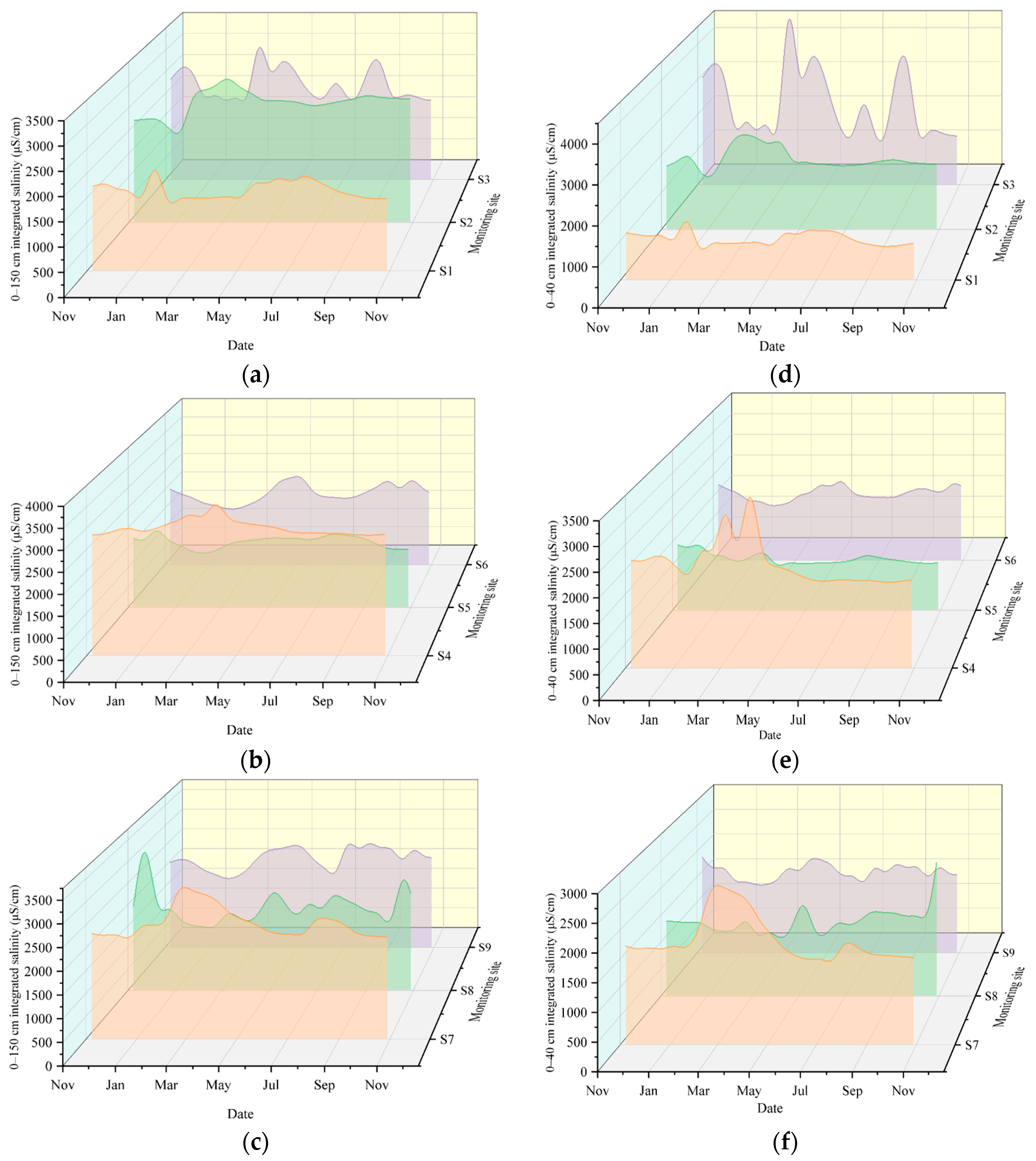
Continuous monitoring data from November 2024 to October 2025 were used to analyze the intra-annual variation in apparent soil EC across the nine monitoring sites. As shown in Figure 3 and

Table 2. Statistical characteristics of integrated EC at 0–40 cm and 0–150 cm.

Site ID	Mean	Median	Maximum	Date of Maximum	Minimum	Date of Minimum	Amplitude	SD	CV
S1	1086.09	1090.85	2093.48	21 January 2025	821.58	31 January 2025	1271.9	208.9	0.192
S1	1702.65	1685.11	2534.67	19 January 2025	1451.03	20 February 2025	1083.65	196.44	0.115
S2	1849.69	1784.62	2566.77	22 March 2025	1388.6	18 January 2025	1178.17	242.18	0.131
S2	2636.32	2677.5	3162.74	14 March 2025	1987.68	7 January 2025	1175.07	262.14	0.099
S3	2291.81	1741.22	5092.78	7 March 2025	1379.71	30 October 2025	3713.08	933.59	0.407
S3	2196.92	1990.41	3138.87	7 March 2025	1817.88	19 January 2025	1321	347.17	0.158
S4	2100.58	1977.13	3688.69	8 April 2025	1726.56	2 October 2025	1962.13	411.42	0.196
S4	3008.31	2939.92	3662.16	8 April 2025	2339.6	6 November 2024	1322.56	176.42	0.059
S5	1127.25	1088.48	1586.72	6 December 2024	976.58	27 March 2025	610.14	122.14	0.108
S5	1645.14	1691.25	2292.36	2 December 2024	1352.54	8 February 2025	939.83	152.93	0.093
S6	1573.03	1576.1	1990.93	6 October 2025	1259.31	28 January 2025	731.62	164.13	0.104
S6	1893.09	1875.93	2604.33	5 October 2025	1473.37	3 February 2025	1130.95	249.16	0.132
S7	1849.48	1687.83	2764.68	5 March 2025	1458.09	24 June 2025	1306.58	404.39	0.219
S7	2555.27	2475.59	3290.5	23 February 2025	2179.13	25 December 2024	1111.36	320.7	0.126
S8	1341.81	1311.73	2484.26	27 October 2025	1000.2	11 April 2025	1484.07	185.05	0.138
S8	1963.69	1892.99	3366.3	27 November 2024	1459.75	31 January 2025	1906.55	438.96	0.224
S9	1604.34	1594.8	2388.21	27 August 2025	1325.96	16 January 2025	1062.25	191.24	0.119
S9	2219.32	2234.86	2908.17	25 July 2025	1694.14	27 January 2025	1214.02	301.48	0.136

Note: The statistical parameters were calculated based on the daily-scale integrated EC series after excluding EC values of zero, obvious high-level or low-level outliers, and initially anomalous low values. The unit of EC is μS/cm. Amplitude is defined as the difference between the maximum and minimum values. CV denotes the coefficient of variation. For each monitoring site, the first row represents the 0–40 cm integrated EC, and the second row represents the 0–150 cm integrated EC.

, apparent EC at all sites exhibited varying degrees of intra-annual fluctuation, characterized by alternating phases of decline, rebound, and subsequent readjustment. Clear differences were observed among monitoring sites in apparent EC levels, fluctuation amplitudes, and the timing of peak values, indicating substantial site-level heterogeneity in apparent soil EC within the monitored farmland.

Figure 3 and Table 2 show substantial differences in integrated apparent EC within the 0–40 cm cultivated layer among monitoring sites. S3 exhibited the highest mean apparent EC in the cultivated layer, at 2291.81 μS/cm, with a maximum of 5092.78 μS/cm and a CV of 0.407, markedly higher than those at the other sites, indicating the strongest fluctuation in cultivated-layer apparent EC. S4 and S7 also showed relatively high apparent EC levels and pronounced intra-annual variability, whereas S1 and S5 generally exhibited lower EC levels. The relatively small CV values at S5 and S6 indicate more stable apparent EC dynamics in the cultivated layer. The timing of maximum EC values also differed among sites, suggesting that high apparent EC in the cultivated layer may be associated with local moisture conditions, the initial salinity background, and field management processes.

Compared with the cultivated layer, integrated apparent EC over the 0–150 cm soil profile was generally higher but exhibited relatively smoother temporal variation. As shown in Table 2, S4 had the highest mean EC_0–150 value, at 3008.31 μS/cm, followed by S2 and S7. At most sites, the CV of EC_0–150 was lower than that of EC_0–40, indicating that short-term fluctuations in integrated apparent EC were weaker at the full-profile scale than in the cultivated layer. S3 was an exception, with a higher mean EC_0–40 than EC_0–150 and a substantially larger CV in the cultivated layer, indicating that apparent EC variability at this site was concentrated mainly in the shallow soil.

Overall, the intra-annual dynamics of farmland apparent EC across the nine monitoring sites exhibited clear site-specific and profile-dependent differences. EC_0–40 was more sensitive to short-term variation, whereas EC_0–150 more strongly reflected the overall apparent EC background of the soil profile. Although their overall directions of change were broadly similar, the two indices differed in fluctuation amplitude, timing of peak values, and temporal stability.

3.2. Stage-Dependent Responses of Soil EC to Hydrothermal Conditions

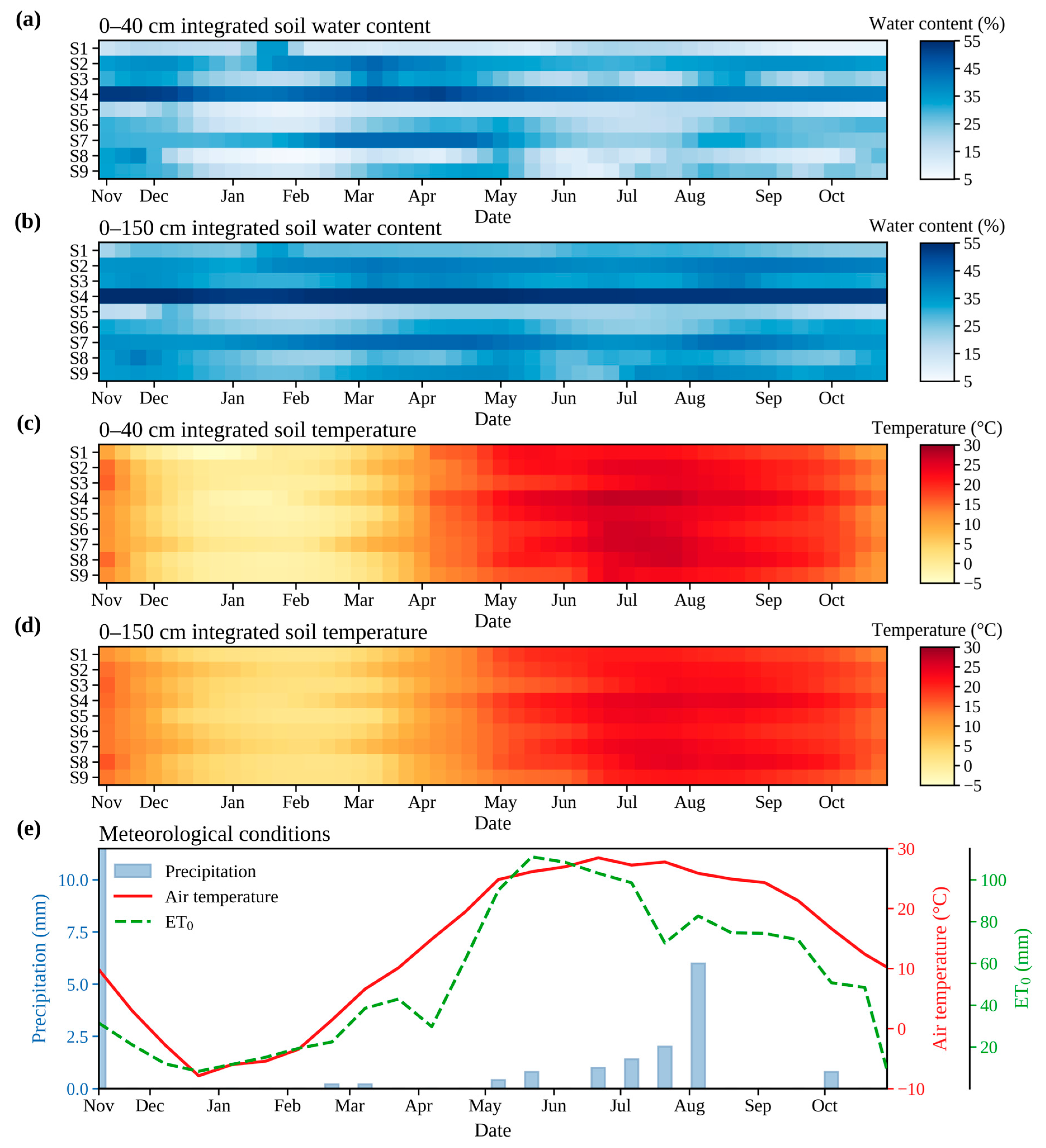
Section 3.1 showed that apparent EC dynamics varied markedly among monitoring sites and exhibited distinct stage-dependent patterns; however, the underlying drivers cannot be determined from the EC trajectories alone. Because the study period covered major field-management stages, including winter irrigation, spring irrigation, and growing-season irrigation, and because event-specific irrigation amounts were unavailable for the individual monitoring sites, soil water content, soil temperature, and meteorological conditions were jointly examined to further characterize the hydrothermal background associated with apparent EC variations. Figure 4 presents the intra-annual dynamics of integrated soil water content, integrated soil temperature, and concurrent meteorological variables at the monitoring sites.

Figure 4 shows clear site-specific differences and temporal fluctuations in integrated soil water content at 0–40 cm. S4 generally exhibited relatively high moisture levels, whereas S5 and S8 remained comparatively low. In contrast, integrated soil water content at 0–150 cm varied more smoothly, indicating that short-term moisture fluctuations were weaker at the full-profile scale than in the cultivated layer. Comparison with the apparent EC patterns in Figure 3 shows that sites with stronger fluctuations in cultivated-layer apparent EC generally also exhibited more pronounced changes in cultivated-layer moisture, suggesting a degree of temporal correspondence between the two. However, this relationship does not establish an independent effect of soil moisture on apparent EC.

Soil temperature and meteorological variables exhibited clear seasonal patterns. Integrated soil temperature at 0–40 cm declined rapidly during winter and gradually increased after spring as air temperature rose, whereas temperature changes at 0–150 cm lagged behind, reflecting the buffering effect of deeper soil layers. Air temperature and ET₀ increased after spring, while precipitation remained generally low, indicating that apparent EC dynamics during the study period occurred under conditions characterized by limited precipitation, relatively strong evapotranspiration demand, and stage-dependent irrigation management.

Taken together, Figure 3 and Figure 4 indicate that stage-dependent changes in apparent soil EC corresponded to variations in soil moisture, temperature, and meteorological conditions. From the period after winter irrigation to early spring, relatively high antecedent moisture and low-temperature conditions coincided with declining or persistently low apparent EC at some sites. After spring, as air temperature and ET₀ increased, moisture and temperature dynamics in the cultivated layer became more active, and apparent EC at some sites showed renewed increases or stronger fluctuations. It should be emphasized that Figure 4 primarily illustrates stage-dependent correspondence between the hydrothermal background and apparent EC dynamics and does not directly quantify the independent contribution of individual factors. Their relative importance is further evaluated below using the model results, with particular attention to model dependence on soil moisture, meteorological deficit, and process-related features.

3.3. Performance Evaluation of the First-Layer Soil Moisture Prediction Model

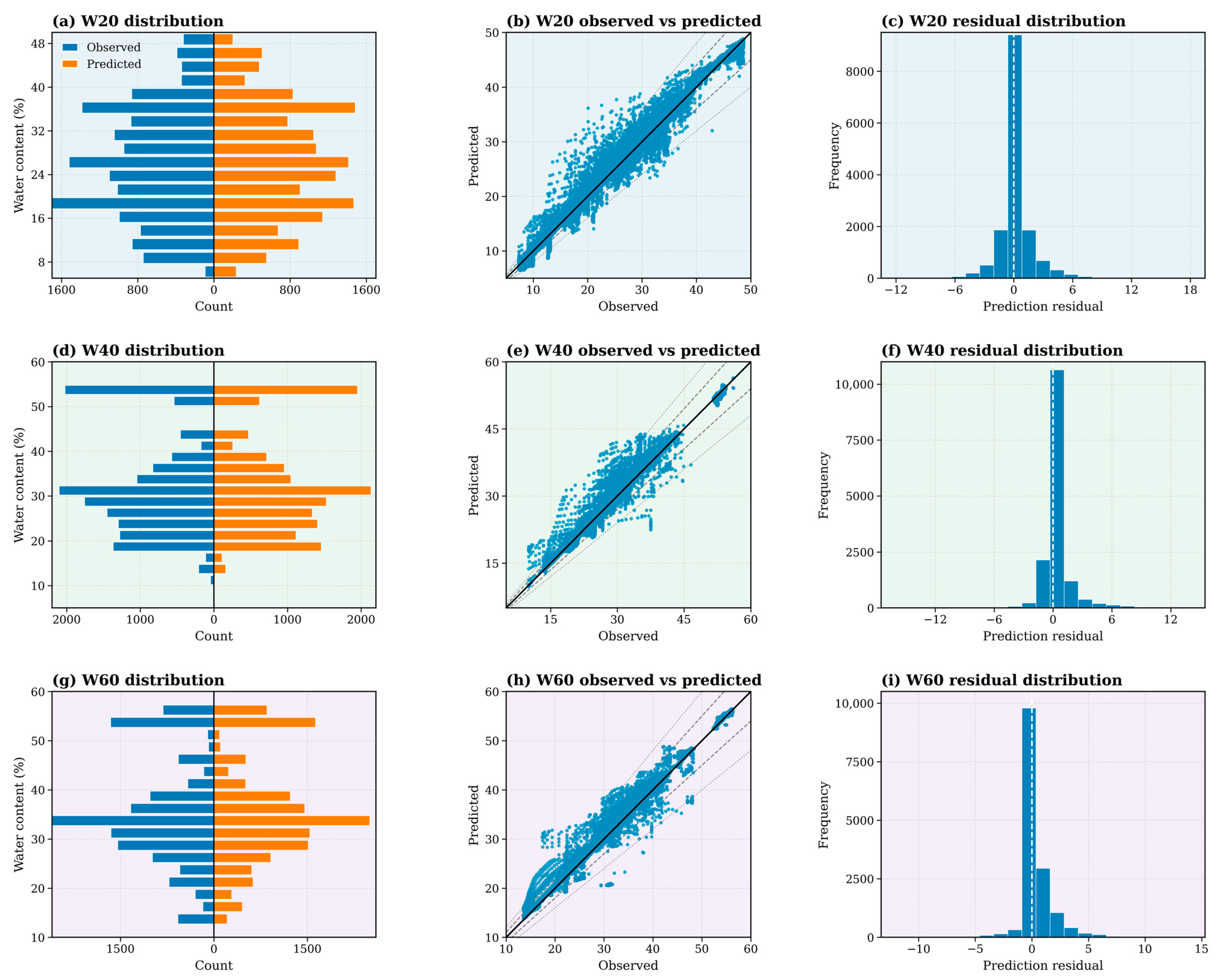
The first-layer model was used to predict future soil moisture states at W₂₀, W₄₀, and W₆₀ during post-irrigation periods without additional irrigation or significant wetting recharge, thereby providing conditional inputs for second-layer apparent EC prediction. The model used soil moisture at initialization, historical moisture changes, profile gradients, soil-temperature background, and point-specific matched ERA5 realized meteorological data as inputs, and was trained using a physical-baseline-assisted machine-learning residual-correction approach. Model performance was evaluated using 5-fold time-forward validation, in which post-irrigation periods were ordered by starting time, earlier samples were used for training, and later samples for validation; soil moisture at initialization was used as the persistence benchmark. Figure 5 presents the distributions of observed and predicted moisture values, fitted relationships, and residual distributions for the three soil depths, while

Table 3. Performance of the first-layer soil moisture prediction model across different prediction windows.

Target	Forecast Window	n	R2	RMSE (%)	MAE (%)	Persistence R2	Skill
W20	0–1 d	5019	0.991	0.93	0.48	0.975	0.65
W20	1–3 d	2959	0.979	1.48	0.88	0.933	0.68
W20	3–7 d	4850	0.968	1.87	1.21	0.881	0.728
W20	7–15 d	2424	0.939	2.82	1.89	0.779	0.722
W40	0–1 d	5019	0.995	0.77	0.26	0.993	0.241
W40	1–3 d	2959	0.988	1.18	0.58	0.979	0.429
W40	3–7 d	4850	0.978	1.72	1	0.954	0.51
W40	7–15 d	2424	0.957	2.72	1.68	0.907	0.538
W60	0–1 d	5019	0.996	0.65	0.22	0.994	0.318
W60	1–3 d	2959	0.987	1.16	0.54	0.98	0.354
W60	3–7 d	4850	0.98	1.56	0.94	0.968	0.38
W60	7–15 d	2424	0.952	2.77	1.82	0.927	0.345

Note: R², RMSE, and MAE were calculated from out-of-fold predictions. Persistence R² represents the coefficient of determination obtained using soil moisture or EC at the initialization time as the predicted future state. Skill denotes the normalized predictive gain of the model relative to the persistence benchmark.

summarizes the quantitative performance across different prediction windows.

As shown in Figure 5, the predicted and observed values of W₂₀, W₄₀, and W₆₀ exhibited generally similar distributions, with most points located close to the 1:1 line and residuals concentrated around zero. These results indicate that the first-layer model effectively characterized soil moisture states at different depths. W₂₀ showed relatively greater dispersion, which may reflect the higher sensitivity of shallow soil moisture to rapid post-irrigation wetting, redistribution, and evapotranspiration. In contrast, the scatter and residual distributions for W₄₀ and W₆₀ were more concentrated, indicating relatively greater prediction stability in the middle and deeper soil layers.

Table 3 shows that the first-layer model achieved high predictive accuracy across all four prediction windows. The R² values for W₂₀, W₄₀, and W₆₀ ranged from 0.939 to 0.991, 0.957 to 0.995, and 0.952 to 0.996, respectively, indicating that the model effectively characterized soil moisture states at different depths within 15 d after irrigation at sites included in the out-of-fold validation. It should be noted that the high R² values partly reflect the strong persistence of soil moisture itself, particularly over short prediction windows and in the middle and deeper soil layers. Therefore, R² alone may overestimate the incremental contribution of the model and should be interpreted together with the persistence benchmark and Skill.

In terms of Skill, the model outperformed the persistence benchmark at all depths and prediction windows. For W₂₀, Skill values were 0.680, 0.728, and 0.722 for the 1–3 d, 3–7 d, and 7–15 d windows, respectively. For W₄₀, Skill increased from 0.241 to 0.538 as the prediction window lengthened. Skill for W₆₀ ranged from 0.318 to 0.380 across the four windows and remained positive overall, although no monotonic increase was observed. These results indicate that the first-layer model not only utilized the initial moisture state at initialization, but also extracted incremental predictive information from historical changes and meteorological conditions beyond that provided by the persistence benchmark. This enables the model to provide out-of-fold moisture-trajectory inputs for second-layer apparent EC prediction. When evaluated using the same samples as the second layer, the R² values for W₂₀, W₄₀, and W₆₀ were 0.952–0.990, 0.962–0.992, and 0.932–0.993, respectively, indicating that the performance differences between the first and second layers were not primarily attributable to differences in evaluation sample size. Detailed results are provided in Supplementary Table S1.

3.4. Performance Evaluation of the Second-Layer Soil EC Prediction Model

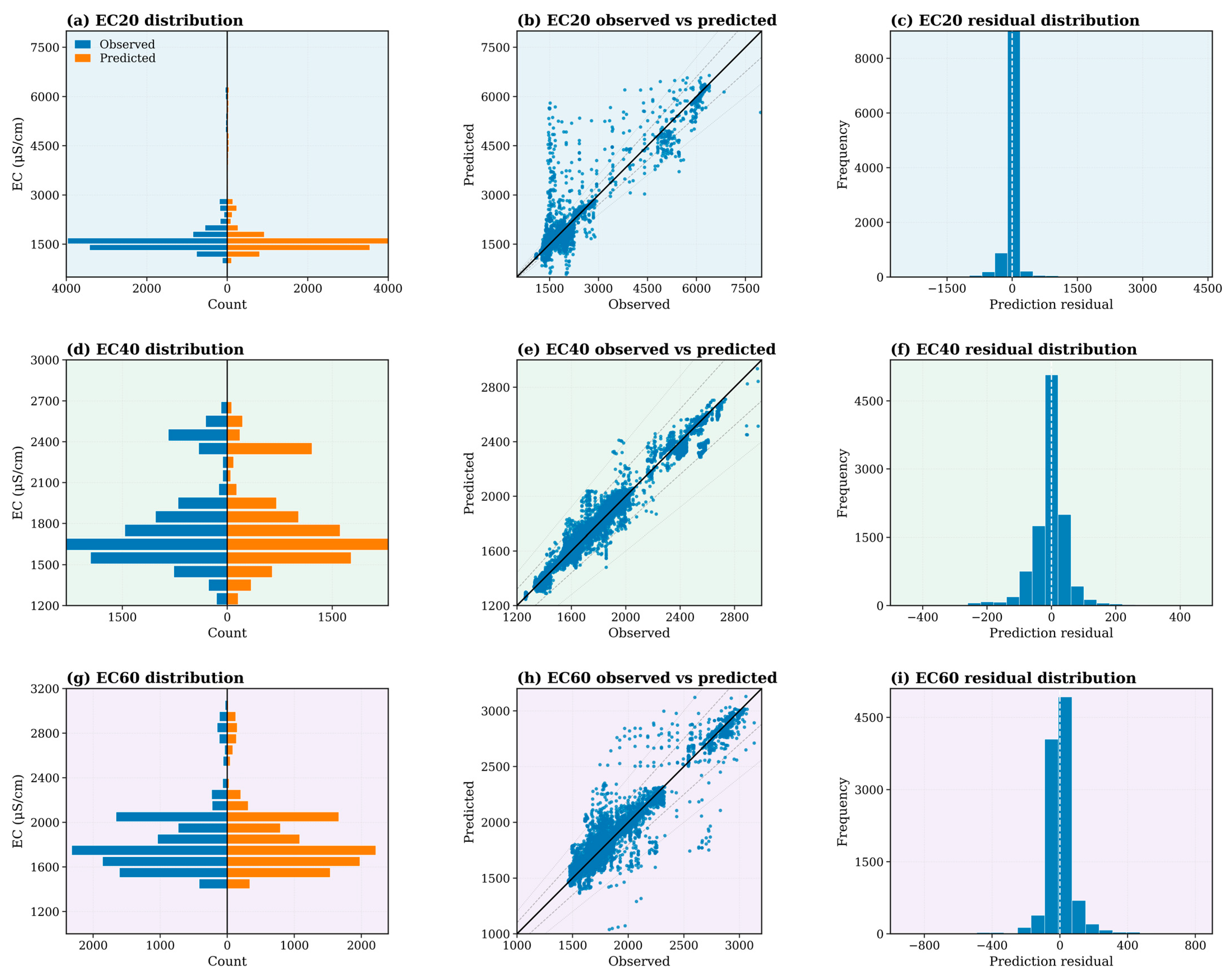
The second-layer model was used to further predict future apparent EC states at EC₂₀, EC₄₀, and EC₆₀ based on the first-layer soil-moisture predictions. Model inputs included the apparent EC background at initialization, historical changes in apparent EC, current soil moisture and temperature states, out-of-fold predicted moisture trajectories from the first layer, and point-specific matched ERA5 realized meteorological data. Apparent EC at the initialization time was used as the persistence benchmark. The second layer used only moisture variables derived from the first-layer out-of-fold predictions and did not use observed future soil moisture, observed future apparent EC, or observed future soil temperature. Figure 6 presents the distributions of observed and predicted apparent EC, their fitted relationships, and prediction-residual distributions at different depths, while

Table 4. Performance of the Second-Layer Apparent Soil EC Prediction Model Across Different Prediction Windows.

Target	Forecast Window	n	R2	RMSE (μS/cm)	MAE (μS/cm)	Persistence R2	Skill
EC20	0–1 d	3605	0.978	126.72	53.12	0.978	−0.001
EC20	1–3 d	2105	0.923	219.88	86.62	0.893	0.277
EC20	3–7 d	3396	0.727	320.71	122.37	0.406	0.54
EC20	7–15 d	1557	−1.376	517.6	185.24	−5.502	0.635
EC40	0–1 d	3614	0.987	34.64	19.69	0.98	0.325
EC40	1–3 d	2111	0.983	41.35	29.43	0.98	0.157
EC40	3–7 d	3406	0.962	65.02	44.09	0.961	0.029
EC40	7–15 d	1566	0.943	89.55	65.28	0.925	0.234
EC60	0–1 d	3614	0.974	47.33	25.06	0.971	0.084
EC60	1–3 d	2111	0.91	88.79	41.31	0.903	0.065
EC60	3–7 d	3406	0.885	101.45	60.31	0.863	0.163
EC60	7–15 d	1566	0.737	158.45	99.81	0.68	0.177

Note: EC₂₀, EC₄₀, and EC₆₀ denote soil electrical conductivity at depths of 20, 40, and 60 cm, respectively. R², RMSE, and MAE were calculated from out-of-fold predictions. Persistence R² represents the coefficient of determination obtained by using soil moisture or EC at the initialization time as the predicted future state. Skill denotes the normalized predictive gain of the model relative to the persistence benchmark. The second-layer sample size was smaller than that of the first layer mainly because the first validation fold was not included in the second-layer evaluation and because EC validity and quality-control screening were applied separately for each target depth.

summarizes the quantitative performance across the different prediction windows.

As shown in Figure 6, the predicted and observed values of EC₂₀, EC₄₀, and EC₆₀ were generally close, indicating that the second-layer model effectively characterized apparent soil EC states at different depths. The scatter distributions of EC₄₀ and EC₆₀ were more concentrated and exhibited narrower residual distributions, indicating greater prediction stability. In contrast, EC20 showed greater dispersion, suggesting that apparent EC in the shallow soil layer was more difficult to predict.

Across the prediction windows, EC₂₀ maintained relatively good predictive performance at 0–1 d, 1–3 d, and 3–7 d, whereas prediction uncertainty increased markedly at 7–15 d. It should be noted that the relatively high R² values for apparent EC prediction were also partly attributable to the initial EC background and strong persistence. Therefore, Skill should be considered together with R² to evaluate the incremental contribution of the model relative to the persistence benchmark. The optimal residual model was selected independently for each soil depth and prediction window. The final selected models included ExtraTrees, RandomForest, XGBoost, and LightGBM, with residual-mixing coefficients α of 0.75 or 1.00, as detailed in Supplementary Table S3.

Table 4 shows clear differences in the predictive performance of the second-layer model across soil depths. EC₄₀ and EC₆₀ maintained relatively high state-prediction accuracy across all prediction windows, with R² values of 0.943–0.987 and 0.737–0.974, respectively, indicating comparatively stable prediction of apparent EC in the middle and deeper soil layers. For EC₂₀, R² values were 0.978, 0.923, and 0.727 for the 0–1 d, 1–3 d, and 3–7 d windows, respectively, indicating that the model could effectively predict shallow-layer apparent EC within 7 d. However, R² declined to −1.376 in the 7–15 d window, indicating that absolute prediction of shallow-layer apparent EC was unreliable over this longer horizon and should not be used for quantitative prediction. In terms of Skill, the incremental advantage over the persistence benchmark varied markedly with soil depth and prediction horizon. EC₂₀ had a Skill of −0.001 at 0–1 d, indicating no improvement over the persistence benchmark. Similarly, Skill values for EC₄₀ at 3–7 d and EC₆₀ at 1–3 d were only 0.029 and 0.065, respectively, indicating weak incremental gains.

For EC₂₀ at 7–15 d, the positive Skill of 0.635 was mainly attributable to the substantially lower R² of the persistence benchmark (−5.502). Although the model reduced prediction error relative to directly using apparent EC at initialization as the future value, the model itself still yielded an R² of −1.376, indicating poor overall agreement between observations and predictions. Therefore, the positive Skill does not demonstrate reliable absolute predictive capability in this window and should be interpreted only as an improvement relative to the persistence benchmark, rather than as evidence of reliable long-horizon quantitative prediction for shallow-layer apparent EC. Because sensor-measured apparent EC is jointly affected by soil water content, temperature, and conductive conditions, these results cannot be used to infer specific mechanisms of salt transport.

Further site-level evaluation showed substantial differences in apparent EC prediction performance among the eight monitoring sites included in out-of-fold validation, and these differences generally increased with prediction horizon. At the longest prediction horizon (7–15 d), site-specific R² values ranged from −8.638 to 0.962 for EC₂₀, from −3.786 to 0.887 for EC₄₀, and from −10.635 to 0.840 for EC₆₀, indicating pronounced site-level heterogeneity. Therefore, the overall R² values reported in Table 4 represent aggregate predictive performance across all validation samples and do not imply identical prediction accuracy at every monitoring site; interpretation should consider both Skill and site-level heterogeneity. Full site-specific R² results across prediction depths and windows are provided in Supplementary Table S2. Paired ablation results further showed that the contribution of the predicted moisture trajectory was strongly depth- and horizon-dependent. Among the 12 depth–window combinations, only EC₂₀ at 3–7 d and EC₆₀ at 7–15 d showed consistent improvements across R², Skill, RMSE, and MAE, with the clearest gain observed for EC₂₀ at 3–7 d (ΔR² = 0.193; ΔSkill = 0.325). For this representative case, RMSE decreased by 23.5% relative to the ablation model, whereas MAE decreased by only 3.9%, suggesting that the gain was more pronounced for larger prediction errors than for typical absolute errors. Across the remaining ten combinations, ΔR² ranged from −0.727 to 0.007; eight showed deterioration across all four metrics, while EC₂₀ at 1–3 d showed slight improvements in R², Skill, and RMSE but worse MAE, and EC₂₀ at 7–15 d showed improved MAE but worse R², Skill, and RMSE. Full paired-ablation results, including R², RMSE, MAE, and Skill changes for all 12 depth–window combinations, are provided in Supplementary Table S4.

3.5. SHAP Feature Dependence and Post-Hoc Scenario Linkage Analysis of Meteorological Deficit

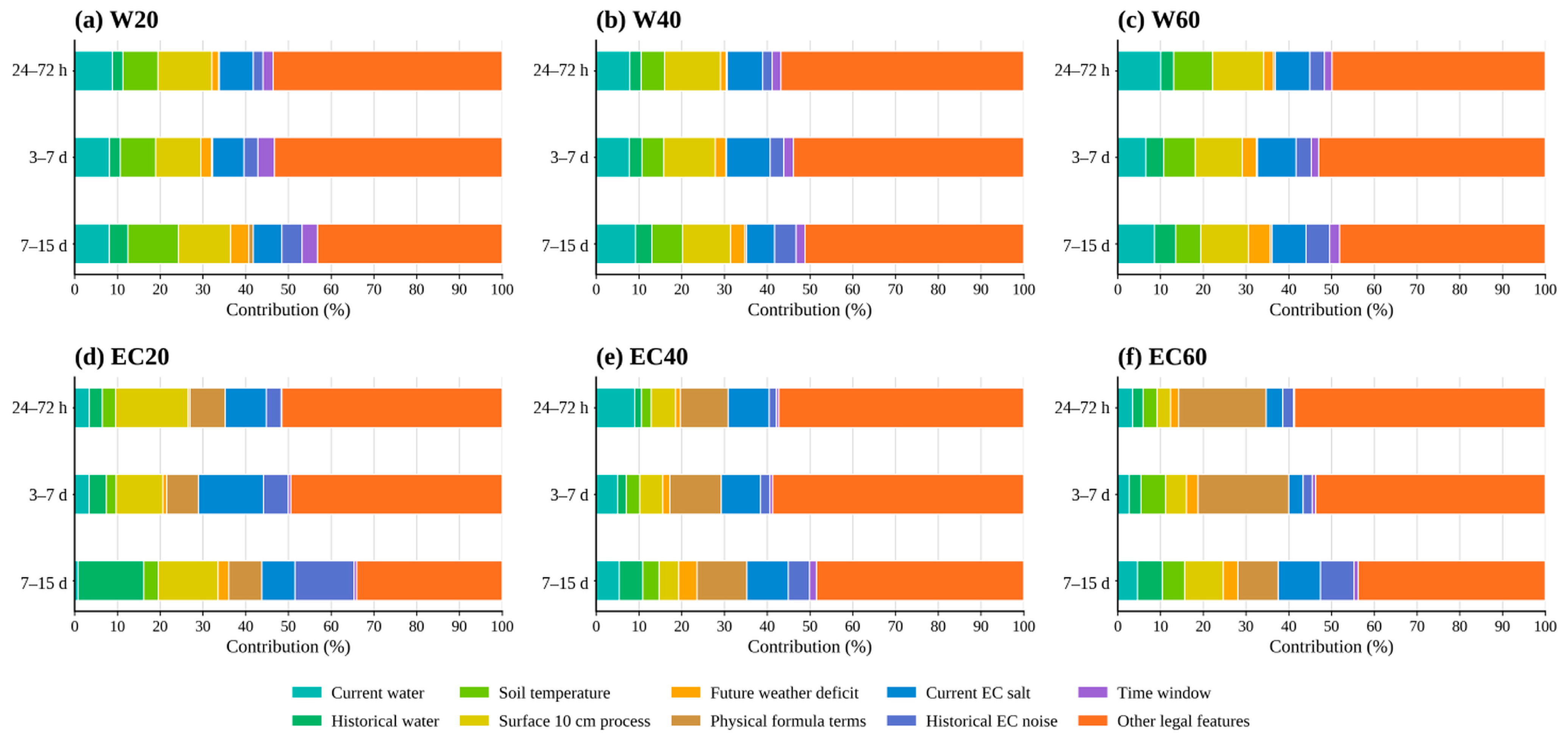
To further clarify the primary information sources underlying model predictions and their local statistical linkage with changes in meteorological deficit, this section analyzes two aspects: SHAP feature-group contributions and post-hoc scenario linkage of meteorological deficit. First, the relative contributions of feature groups were compared across different prediction windows for W₂₀, W₄₀, W₆₀, EC₂₀, EC₄₀, and EC₆₀ to evaluate model dependence on current states, historical changes, predicted moisture trajectories, physical-baseline terms, meteorological conditions, and related information. Second, local linear relationships among meteorological deficit, predicted moisture changes, and apparent EC changes were established based on out-of-fold predictions, and different meteorological-deficit scenarios were imposed within these local relationships to compare the direction and magnitude of associated changes in apparent EC at different depths. These results reflect only model dependence and statistical sensitivity and should not be interpreted as direct evidence of causal relationships among variables or actual water–salt transport mechanisms. The relative SHAP contributions of feature groups for different prediction targets and prediction windows are shown in Figure 7.

As shown in Figure 7, the mean contribution of the other eligible features was 51.43% in the first-layer moisture model and 50.55% in the second-layer apparent EC model. This feature group mainly included monitoring-site background, temporal encoding, prediction horizon, statistical background at initialization, and auxiliary variables constructed using information available at or before the initialization time. In the second layer, it also included the first-layer out-of-fold predicted moisture trajectories and their associated change features. The relatively high contribution of this feature group indicates strong model dependence on these inputs, but does not imply causal effects or the use of observed future values or other post-hoc information.

In the first-layer moisture model, the mean contributions of the 10 cm surface-layer process features, current soil moisture, current apparent EC background, and soil-temperature background were 11.74%, 8.34%, 8.00%, and 7.61%, respectively, indicating substantial model dependence on the initial moisture state, shallow-layer hydrothermal information, and apparent EC background. The mean contribution of the physical-formula terms in the first layer was 0.39%, indicating a relatively small direct SHAP contribution in the current model; these terms mainly served as auxiliary components of the physical baseline. This result does not imply that the corresponding physical processes themselves are unimportant.

In the second-layer apparent EC model, the first-layer out-of-fold predicted moisture trajectory was an important source of information. To further evaluate its role, variables related to the predicted moisture trajectory within the “other eligible features” group were summarized separately. Sample-level SHAP results showed that, within the 0–1 d window, the relative contributions of the predicted moisture trajectory to EC₂₀, EC₄₀, and EC₆₀ were 39.2%, 37.6%, and 26.8%, respectively, indicating that short-term apparent EC prediction depended strongly on the future moisture states and changes provided by the first layer. As the prediction window increased, the relative roles of the predicted moisture trajectory and physical-baseline terms diverged. For EC₂₀, the model remained primarily dependent on the predicted moisture trajectory and physical-baseline terms over the 1–15 d windows, with their combined contribution ranging from approximately 65.7% to 67.7%. For EC₄₀, the physical-baseline terms dominated the 3–7 d and 7–15 d windows, contributing 67.0% and 63.0%, respectively. For EC₆₀, dependence on the predicted moisture trajectory remained relatively high over 0–7 d, whereas the contribution of the physical-baseline terms increased to 65.5% in the 7–15 d window. These results indicate that the second-layer model showed clear dependence on the first-layer predicted moisture trajectory and that this dependence varied with soil depth and prediction horizon; whether such dependence translated into actual predictive improvement was further assessed using the paired ablation results.

As shown in

Table 5. Changes in Apparent Soil EC Across Prediction Windows Under Different Post-Hoc Meteorological-Deficit Scenarios.

Scenario	Target	0–1 d	1–3 d	3–7 d	7–15 d
Meteorological deficit increased by 20%	EC20	−2.23	−8.01	−21.11	−36.25
Meteorological deficit increased by 20%	EC40	1.18	0.78	4.78	8.4
Meteorological deficit increased by 20%	EC60	0.28	−3.69	−4.64	5.2
Meteorological deficit decreased by 20%	EC20	2.23	8.01	21.11	36.25
Meteorological deficit decreased by 20%	EC40	−1.18	−0.78	−4.78	−8.4
Meteorological deficit decreased by 20%	EC60	−0.28	3.69	4.64	−5.2
Meteorological deficit decreased by 40%	EC20	4.47	16.01	42.23	72.5
Meteorological deficit decreased by 40%	EC40	−2.36	−1.57	−9.56	−16.8
Meteorological deficit decreased by 40%	EC60	−0.56	7.39	9.27	−10.41

, under the established local linear relationships, the associated changes in apparent EC under different meteorological-deficit scenarios were generally small, although both the direction and magnitude varied with soil depth and prediction window. Under the scenario of a 20% increase in meteorological deficit, the predicted change in EC₂₀ ranged from −2.23 to −36.25 μS/cm, indicating that the magnitude of the decrease increased from 2.23 to 36.25 μS/cm. EC₄₀ increased slightly by 0.78–8.40 μS/cm across the prediction windows, whereas EC₆₀ changed by −4.64 to 5.20 μS/cm. These results reflect only the local sensitivity of the model to meteorological-deficit inputs and cannot be used to infer independent causal effects or specific water–salt transport processes under actual field conditions.

EC₂₀ showed a negative response under the 20% increase in meteorological deficit, but this result should not be interpreted as an actual decrease in shallow-layer soil salinity. Sensor-measured apparent EC is jointly affected by soil water content, pore-water conditions, and the continuity of conductive pathways. Therefore, the decrease in model-predicted EC may reflect statistical dependence on moisture-sensitive apparent-conductivity characteristics and cannot distinguish the relative contributions of changes in salt concentration and conductive conditions. In particular, because the baseline predictive performance of EC₂₀ at 7–15 d was unreliable, the negative response in this window is reported only to describe changes in model output and is not used for quantitative or mechanistic interpretation.

Under the 20% decrease and 20% increase in meteorological deficit scenarios, the associated changes in apparent EC at each depth were opposite in direction but approximately equal in magnitude, whereas the magnitude of change under the 40% decrease scenario was approximately twice that under the 20% decrease scenario. This proportional relationship mainly results from the local linear linkage calculation and does not imply a strictly linear response of the complete two-layer prediction model. Overall, this analysis is intended only to support interpretation of the statistical linkages among meteorological deficit, predicted moisture changes, and depth-specific apparent EC.

4. Discussion

4.1. Intra-Annual Differentiation of Farmland Apparent EC and Determination of Depth-Specific Prediction Targets

Previous studies have shown that variations in apparent soil EC in farmland within arid irrigation districts do not solely reflect salt accumulation, but are also associated with irrigation recharge, evapotranspiration demand, crop water uptake, and soil-profile water redistribution [29]. After irrigation, water infiltration may alter shallow-layer soil moisture and apparent EC, whereas during irrigation intervals, the development of soil water deficits may lead to differentiated changes in apparent EC among soil depths [30]. Changes in shallow-layer hydrothermal exchange under mulching may also result in different apparent EC responses between shallow and deeper soil layers [31]. In addition, soil texture affects water retention, infiltration, and electrical conductivity characteristics, and may therefore contribute to differences in apparent EC levels and fluctuation amplitudes among monitoring sites [32].

The results of this study are generally consistent with these findings. Integrated apparent EC at both 0–40 cm and 0–150 cm exhibited clear site-specific differences and stage-dependent variations, but the two indices represent different spatial scales. Integrated apparent EC at 0–40 cm showed stronger intra-annual fluctuations and greater sensitivity to changes in shallow-layer hydrothermal conditions, making it suitable for characterizing rapid changes in apparent EC within the cultivated layer. In contrast, integrated apparent EC at 0–150 cm was more strongly influenced by the deeper-soil background and the smoothing effect of soil-layer-thickness weighting, resulting in weaker short-term fluctuations and making it more suitable for representing the overall apparent EC status of the soil profile. In combination with Table 1, differences in soil texture among sites may be one factor contributing to variations in apparent EC background and fluctuation amplitude; however, the available data are insufficient for quantitative attribution. Therefore, integrated apparent EC indices are appropriate for describing intra-annual variation, site-level differences, and profile differentiation of apparent EC in the study area.

However, integrated apparent EC also has limitations when used as a prediction target during post-irrigation periods without additional irrigation or significant wetting events. Because the 0–40 cm and 0–150 cm integrated indices are weighted by soil-layer thickness, short-term changes in apparent EC within individual soil layers may be smoothed. If integrated apparent EC were retained as the primary prediction target, the model might achieve relatively high overall state-prediction accuracy, but its performance could be strongly influenced by the initial state and profile-averaging effects, thereby obscuring depth-specific changes across the 0–1 d, 1–3 d, 3–7 d, and 7–15 d prediction windows.

Accordingly, the prediction targets were further specified as W₂₀, W₄₀, W₆₀, EC₂₀, EC₄₀, and EC₆₀ for model evaluation. This treatment does not negate the utility of the integrated indices, but rather distinguishes their respective roles: integrated apparent EC is used to characterize intra-annual variation and the overall profile background, whereas depth-specific indices are used to evaluate soil moisture and apparent EC changes at different depths during post-irrigation prediction windows. Specifically, W₂₀ and EC₂₀ primarily represent shallow-layer changes, W₄₀ and EC₄₀ characterize middle-layer changes, and W₆₀ and EC₆₀ describe changes in the middle-to-deeper soil layer. Differences among depths may be related to surface hydrothermal exchange, root-zone water use, and profile redistribution; however, the present results are insufficient to establish the independent causal effects of these processes.

4.2. Role of First-Layer Predicted Moisture Trajectories in Conditional Prediction of Apparent EC

Previous studies have shown that apparent soil EC is not directly equivalent to soil salt content; rather, its variation is jointly influenced by soil water content, temperature, pore-water connectivity, and the continuity of conductive pathways [32]. Irrigation infiltration, evapotranspirative water loss, profile water redistribution, and capillary recharge may induce concurrent changes in soil moisture status, ionic conduction conditions, and apparent EC [33]. Under mulched drip irrigation, water inputs are highly localized and spatially heterogeneous, and the hydrothermal conditions and apparent EC responses of different soil layers often exhibit pronounced spatial and depth-dependent differences [34]. Therefore, post-irrigation increases or decreases in apparent EC cannot be attributed simply to gains or losses of soil water, but should be interpreted in conjunction with the initial apparent EC background, subsequent moisture trajectories, and soil-depth differences [35].

Based on this understanding, the role of the first-layer moisture model is not limited to predicting future W₂₀, W₄₀, and W₆₀ states, but also includes providing continuous moisture-condition information to the second-layer model. The second layer uses the out-of-fold predicted moisture trajectories generated by the first layer to construct variables describing predicted moisture states, moisture changes, and interlayer moisture differences. These variables are derived from information available at or before initialization together with meteorological conditions over the target period, and do not include observed soil moisture or apparent EC at the target time, thereby avoiding leakage of future observations. The second-layer model further combines apparent EC at initialization, historical changes, meteorological deficit, and related interaction variables to conditionally predict apparent EC at different depths and prediction windows. The physical-baseline terms provide structured process-based references, whereas the residual models correct nonlinear deviations and site-specific differences not captured by the baseline.

The first-layer model achieved high state-prediction R² values across all prediction windows, although these values also partly reflect the temporal persistence of soil moisture. Therefore, the persistence benchmark and Skill were additionally used to evaluate incremental predictive capability. W₂₀, W₄₀, and W₆₀ all achieved positive Skill across the prediction windows. W₂₀ maintained relatively high gains, the gain for W₄₀ generally increased with prediction horizon, and W₆₀ remained comparatively stable. These results indicate that, beyond the initial moisture state, the first-layer model extracted additional information from historical moisture changes, meteorological deficit, and profile conditions, thereby providing the second layer with predicted moisture states and trajectory information beyond that contained in the persistence benchmark.

The SHAP results of the second-layer model further indicate that the first-layer out-of-fold predicted moisture trajectory was not merely an intermediate variable within the two-layer structure. Within the 0–1 d window, its relative contributions to EC₂₀, EC₄₀, and EC₆₀ were 39.2%, 37.6%, and 26.8%, respectively. Over the 1–15 d windows, the combined dependence of EC₂₀ on the predicted moisture trajectory and physical-baseline terms was 65.7–67.7%. For EC₄₀, the physical-baseline terms contributed 67.0% and 63.0% in the 3–7 d and 7–15 d windows, respectively. EC₆₀ depended more strongly on the predicted moisture trajectory over 0–7 d, whereas the contribution of the physical-baseline terms increased to 65.5% in the 7–15 d window. These findings demonstrate a quantifiable dependence of the second-layer model on the first-layer predicted moisture trajectory. However, such model dependence does not necessarily translate into consistent predictive gain, and its actual contribution must be interpreted together with the paired ablation results. Nor should it be regarded as causal evidence that moisture changes drive salt transport.

Clear differences in apparent EC predictive performance were observed among soil depths. EC₄₀ and EC₆₀ remained generally stable across prediction windows, whereas the R² for EC₂₀ declined to −1.376 in the 7–15 d window, indicating unreliable absolute predictive performance. Although this window yielded a positive Skill of 0.635, this mainly resulted from the poorer performance of the persistence benchmark, for which R² was −5.502. Therefore, the positive Skill should not be interpreted as evidence of reliable long-term prediction of shallow-layer apparent EC. Shallow apparent EC is highly sensitive to changes in soil water content and conductive conditions, and its decline may reflect changes in pore water and conductive pathways as well as possible effects of salt redistribution; the available data cannot separate the independent contributions of these factors. From the perspective of model structure, the principal role of the two-layer framework is to incorporate the predicted moisture trajectory as a conditional input for second-layer apparent EC prediction. Paired ablation results further showed that this input did not yield consistent gains across all depths and prediction horizons. The clearest improvement occurred for EC₂₀ at 3–7 d, whereas some other windows exhibited trade-offs among evaluation metrics. Therefore, the first-layer predicted moisture trajectory provides conditional incremental value for second-layer prediction, and the hypothesis regarding its incremental contribution is only partially supported. Although the physical baseline and two-layer information transfer improve process interpretability, the resulting evidence primarily reflects internal model dependence and predictive associations and cannot be directly interpreted as causal evidence of actual water–salt transport mechanisms. Because data on root distribution, depth-specific root water uptake, and complete irrigation inputs were unavailable, crop water consumption and root-zone processes could only be represented indirectly through variables such as ET₀, historical moisture changes, and predicted moisture gradients.

4.3. Interpretation of SHAP Results and Meteorological-Deficit Linkages

Previous studies have applied cascaded machine-learning approaches in which predicted soil moisture is used as an input to salinity models [36], thereby providing information on changes in soil moisture conditions for salinity prediction. In this study, this concept was applied to farmland in an arid irrigation district by using the first-layer out-of-fold predicted moisture trajectory as a conditional input to the second-layer apparent EC model. SHAP analysis and post-hoc scenario linkage analysis of meteorological deficit were then used to evaluate model dependence on different types of input information and their local statistical linkages. It should be emphasized that these analyses were intended to interpret internal model relationships rather than to identify causal mechanisms of specific water–salt processes.

The SHAP results showed that both the first-layer moisture model and the second-layer apparent EC model depended on multiple types of input information. The first-layer model primarily used the initial moisture state, historical changes, shallow-layer hydrothermal information, and meteorological deficit, whereas the second-layer model further incorporated the first-layer predicted moisture trajectory, the apparent EC background at initialization, and variables related to the physical baseline. The relative contributions of different feature groups varied across soil depths and prediction windows, indicating that apparent EC prediction was not determined by any single variable. The relatively high contribution of the first-layer predicted moisture trajectory in the second layer indicates substantial model dependence on this information; however, whether this dependence translated into actual predictive gain must be assessed together with the paired ablation results. Similarly, SHAP values cannot be used to infer the independent effect of moisture changes on salt transport.

The post-hoc scenario linkage analysis showed that, under the established local linear relationships, the associated changes in apparent EC were generally limited in magnitude, although both their direction and magnitude varied with soil depth and prediction window. Under a 20% increase in meteorological deficit, predicted EC₂₀ changed by −2.23 to −36.25 μS/cm across the 0–1 d to 7–15 d windows; EC₄₀ showed small increases of 0.78–8.40 μS/cm; and the direction of EC₆₀ changes varied among prediction windows. These results indicate that the model exhibited some local sensitivity to meteorological-deficit inputs, but they do not establish meteorological deficit as an independent dominant factor controlling apparent EC. Comparison with the prediction errors reported in Table 4 further showed that, under the 40% decrease in meteorological deficit, the absolute associated changes in apparent EC ranged from 0.56 to 72.50 μS/cm across depths and prediction windows, whereas the corresponding model RMSE values ranged from 34.64 to 517.60 μS/cm. The post-hoc scenario-linked changes were therefore approximately 1.2–18.8% of the corresponding RMSE values and were generally much smaller than the model’s own prediction errors. Accordingly, these post-hoc scenario linkage results are primarily useful for characterizing local statistical associations between model predictions and changes in meteorological deficit and do not yet demonstrate clear practical management significance.

Under the 20% and 40% decreases in meteorological deficit, the predicted changes at each depth were generally opposite in direction to those under the 20% increase scenario, and the magnitude of change under the 40% decrease scenario was approximately twice that under the 20% decrease scenario, consistent with the imposed scenario amplitudes. Therefore, these results mainly reflect the numerical response of the model within the current sample domain and local scenario range and do not imply that apparent EC in actual field conditions responds linearly or symmetrically to meteorological conditions. Because the baseline prediction R² for EC₂₀ at 7–15 d was −1.376, the post-hoc scenario linkage result for this window is reported only to describe changes in model output and does not support reliable quantitative interpretation.

Overall, the SHAP and post-hoc meteorological-deficit scenario linkage analyses jointly indicate that second-layer apparent EC prediction depends on a combination of the apparent EC background at initialization, the first-layer predicted moisture trajectory, and variables related to the physical baseline. These two analyses improve the interpretability of the model results, but their scope is limited to model dependence and input sensitivity and cannot substitute for independent observations or causal validation of actual water–salt transport processes.

4.4. Model Applicability Boundaries and Future Improvements

The physical-baseline-assisted two-layer residual-corrected conditional prediction model for soil moisture and apparent EC developed in this study is primarily intended for depth-specific prediction of soil moisture and apparent EC during post-irrigation periods without additional irrigation or significant wetting recharge. Soil moisture, temperature, and apparent EC at the end of a wetting event are used as the initialization conditions, and rolling predictions are conducted over four windows: 0–1 d, 1–3 d, 3–7 d, and 7–15 d. When a new irrigation or significant wetting event occurs, the ongoing prediction is terminated and reinitialized using the updated soil state. This framework does not require event-specific measured irrigation amounts and is therefore applicable to farmland where irrigation records are incomplete but continuous multi-depth monitoring of soil water, salinity, and temperature is available.

The first-layer moisture model provides incremental predictive information beyond the initial moisture state, while the second-layer model further uses the first-layer out-of-fold predicted moisture trajectories, apparent EC at initialization, and variables related to the physical baseline to conditionally predict apparent EC at different soil depths. Accordingly, the model can support evaluation of depth-specific changes in soil moisture and apparent EC after irrigation. However, it cannot be used to directly identify specific processes such as salt leaching, transport, or accumulation, nor can it replace information on irrigation amount, soil properties, and crop conditions required for field irrigation management.

The current model is applicable only under unfrozen-soil conditions and when no additional irrigation or significant wetting recharge occurs within 15 d after initialization. For EC₂₀ at 7–15 d, R² was −1.376, indicating unreliable absolute predictive performance; therefore, this window is not suitable for quantitative interpretation. The model is also not applicable during soil freezing or pronounced freeze–thaw transitions, because changes in water phase and disruption of conductive pathways may substantially affect sensor measurements of soil moisture and apparent EC. In addition, the present study used ERA5 reanalysis data that had already been realized during the target period. Therefore, the reported performance represents retrospective conditional prediction under observed meteorological forcing. For real-time forecasting applications, weather-forecast data would need to be incorporated, and the influence of forecast uncertainty on model performance would require reevaluation.

The available dataset lacks complete event-specific irrigation amounts, irrigation-water chemistry, fertilization records, root distribution, depth-specific root water uptake, and systematic soil hydraulic parameters. In addition, the available soil information mainly consists of depth-specific texture data and lacks the complete diagnostic information required for WRB classification; therefore, the monitoring sites were not assigned WRB soil classes. This limitation also restricts further interpretation of model differences among soil types. Consequently, the independent effects of individual factors on soil moisture and apparent EC dynamics cannot be separated. The model has not yet been externally validated across independent years, new monitoring sites, or other irrigation districts. Future work should incorporate weather forecasts, groundwater-table depth, irrigation-water EC, root-zone processes, and multi-year monitoring data, together with cross-site and cross-year validation. The framework may be applicable to farmland with comparable monitoring conditions, but local calibration and validation remain necessary before application to new regions or different management systems.

5. Conclusions

This study analyzed the intra-annual variation and profile differentiation of apparent soil EC using multi-depth continuous monitoring data on soil water, salinity, and temperature from nine farmland sites in the Bachu irrigation district, together with point-specific matched hourly ERA5 meteorological data. A physical-baseline-assisted two-layer residual-corrected conditional prediction model for soil moisture and apparent EC was then developed for post-irrigation periods without additional irrigation or significant wetting events. The main conclusions are as follows:

• Apparent soil EC in the study area exhibited clear site-specific differences and vertical profile differentiation. Integrated apparent EC at 0–40 cm showed relatively strong intra-annual fluctuations and was suitable for characterizing short-term changes in the cultivated layer, whereas integrated apparent EC at 0–150 cm varied more smoothly because of the influence of deeper-soil background conditions and the smoothing effect of soil-layer-thickness weighting, making it more suitable for representing the overall profile background. Thus, integrated and depth-specific indices are better suited to describing overall soil conditions and short-term changes at individual depths, respectively.
• The first-layer model effectively predicted future W₂₀, W₄₀, and W₆₀ states during post-irrigation periods without additional wetting recharge. Across the prediction windows, R² values ranged from 0.939 to 0.991, 0.957 to 0.995, and 0.952 to 0.996 for W₂₀, W₄₀, and W₆₀, respectively, and Skill remained positive in all cases. These results indicate that, beyond the initial moisture state, the model extracted incremental predictive information relative to the persistence benchmark and provided moisture-condition inputs for second-layer apparent EC prediction.
• The second-layer model achieved depth-specific conditional prediction of apparent EC using the first-layer out-of-fold predicted moisture trajectories. Prediction performance for EC₄₀ and EC₆₀ was generally stable, with R² values of 0.943–0.987 and 0.737–0.974, respectively, although the incremental advantage over the persistence benchmark was weak in some windows. For EC₂₀, R² values were 0.978, 0.923, and 0.727 for the 0–1 d, 1–3 d, and 3–7 d windows, respectively, with corresponding Skill values of −0.001, 0.277, and 0.540. Although the 7–15 d window yielded a positive Skill of 0.635, R² declined to −1.376, indicating that absolute predictive performance remained unreliable. Paired ablation results showed that the incremental contribution of the first-layer predicted moisture trajectory was strongly dependent on soil depth and prediction horizon. The clearest improvement occurred for EC₂₀ at 3–7 d, while EC₆₀ at 7–15 d showed a modest improvement; most other depth–horizon combinations did not exhibit consistent gains. SHAP and post-hoc meteorological-deficit scenario linkage analyses further showed that the model had quantifiable dependence on predicted moisture trajectories and related process information, but these results should not be interpreted as causal evidence of actual water–salt transport mechanisms.

References

1. Zhang, Y.; Li, X.; Šimůnek, J.; Shi, H.; Chen, N.; Hu, Q. Quantifying Water and Salt Movement in a Soil–Plant System of a Corn Field Using HYDRUS (2D/3D) and the Stable Isotope Method. Agric. Water Manag. 2023, 288, 108492. [Google Scholar] [CrossRef] [Scilit]
2. Li, Y.; Yu, Q.; Ning, H.; Gao, Y.; Sun, J. Simulation of Soil Water, Heat, and Salt Adsorptive Transport Under Film Mulched Drip Irrigation in an Arid Saline-Alkali Area Using HYDRUS-2D. Agric. Water Manag. 2023, 290, 108585. [Google Scholar] [CrossRef] [Scilit]
3. Wang, R.; Kang, Y.; Wan, S.; Hu, W.; Liu, S.; Jiang, S.; Liu, S. Influence of Different Amounts of Irrigation Water on Salt Leaching and Cotton Growth under Drip Irrigation in an Arid and Saline Area. Agric. Water Manag. 2012, 110, 109–117. [Google Scholar] [CrossRef] [Scilit]
4. Liu, M.; Yang, J.; Li, X.; Liu, G.; Yu, M.; Wang, J. Distribution and Dynamics of Soil Water and Salt Under Different Drip Irrigation Regimes in Northwest China. Irrig. Sci. 2013, 31, 675–688. [Google Scholar] [CrossRef] [Scilit]
5. Nachshon, U.; Weisbrod, N.; Dragila, M.I.; Grader, A. Combined Evaporation and Salt Precipitation in Homogeneous and Heterogeneous Porous Media. Water Resour. Res. 2011, 47, W03513. [Google Scholar] [CrossRef] [Scilit]
6. Ning, S.; Zhou, B.; Shi, J.; Wang, Q. Soil Water/Salt Balance and Water Productivity of Typical Irrigation Schedules for Cotton Under Film Mulched Drip Irrigation in Northern Xinjiang. Agric. Water Manag. 2021, 245, 106651. [Google Scholar] [CrossRef] [Scilit]
7. Qi, Z.; Feng, H.; Zhao, Y.; Zhang, T.; Yang, A.; Zhang, Z. Spatial Distribution and Simulation of Soil Moisture and Salinity Under Mulched Drip Irrigation Combined with Tillage in an Arid Saline Irrigation District, Northwest China. Agric. Water Manag. 2018, 201, 219–231. [Google Scholar] [CrossRef] [Scilit]
8. Wang, Y.; Gao, M.; Chen, H.; Fu, X.; Wang, L.; Wang, R. Soil Moisture and Salinity Dynamics of Drip Irrigation in Saline-Alkali Soil of Yellow River Basin. Front. Environ. Sci. 2023, 11, 1130455. [Google Scholar] [CrossRef] [Scilit]
9. Yang, T.; Cherchian, S.; Liu, X.; Shahrokhnia, H.; Mo, M.; Šimůnek, J.; Wu, L. Effect of Water Application Methods on Salinity Leaching Efficiency in Different Textured Soils Based on Laboratory Measurements and Model Simulations. Agric. Water Manag. 2023, 281, 108250. [Google Scholar] [CrossRef] [Scilit]
10. Togneri, R.; dos Santos, D.F.; Camponogara, G.; Nagano, H.; Custodio, G.; Prati, R.; Fernandes, S.; Kamienski, C. Soil Moisture Forecast for Smart Irrigation: The Primetime for Machine Learning. Expert Syst. Appl. 2022, 207, 117653. [Google Scholar] [CrossRef] [Scilit]
11. Wang, Z.; Fan, B.; Guo, L. Soil Salinization after Long-Term Mulched Drip Irrigation Poses a Potential Risk to Agricultural Sustainability. Eur. J. Soil Sci. 2019, 70, 20–24. [Google Scholar] [CrossRef] [Scilit]
12. Sun, L.; Chang, X.; Yu, X.; Jia, G.; Chen, L.; Wang, Y.; Liu, Z. Effect of Freeze-Thaw Processes on Soil Water Transport of Farmland in a Semi-Arid Area. Agric. Water Manag. 2021, 252, 106876. [Google Scholar] [CrossRef] [Scilit]
13. Bing, H.; He, P.; Zhang, Y. Cyclic Freeze-Thaw as a Mechanism for Water and Salt Migration in Soil. Environ. Earth Sci. 2015, 74, 675–681. [Google Scholar] [CrossRef] [Scilit]
14. Li, Z.; Liu, X.; Zhang, X.; Li, W. Infiltration of Melting Saline Ice Water in Soil Columns: Consequences on Soil Moisture and Salt Content. Agric. Water Manag. 2008, 95, 498–502. [Google Scholar] [CrossRef] [Scilit]
15. Li, L.; Liu, H.; He, X.; Lin, E.; Yang, G. Winter Irrigation Effects on Soil Moisture, Temperature and Salinity, and on Cotton Growth in Salinized Fields in Northern Xinjiang, China. Sustainability 2020, 12, 7573. [Google Scholar] [CrossRef] [Scilit]
16. Hou, R.; Li, T.; Fu, Q.; Liu, D.; Li, M.; Zhou, Z.; Yan, J.; Zhang, S. Research on the Distribution of Soil Water, Heat, Salt and Their Response Mechanisms under Freezing Conditions. Soil Tillage Res. 2020, 196, 104486. [Google Scholar] [CrossRef] [Scilit]
17. Corwin, D.L.; Scudiero, E. Review of Soil Salinity Assessment for Agriculture across Multiple Scales Using Proximal and/or Remote Sensors. Adv. Agron. 2019, 158, 1–130. [Google Scholar] [CrossRef] [Scilit]
18. Noborio, K. Measurement of Soil Water Content and Electrical Conductivity by Time Domain Reflectometry: A Review. Comput. Electron. Agric. 2001, 31, 213–237. [Google Scholar] [CrossRef] [Scilit]
19. Scudiero, E.; Corwin, D.L.; Anderson, R.G.; Skaggs, T.H. Moving Forward on Remote Sensing of Soil Salinity at Regional Scale. Front. Environ. Sci. 2016, 4, 65. [Google Scholar] [CrossRef] [Scilit]
20. Lazarovitch, N.; Kisekka, I.; Oker, T.E.; Brunetti, G.; Wöhling, T.; Li, X.; Li, Y.; Skaggs, T.H.; Furman, A.; Sasidharan, S.; et al. Modeling of Irrigation and Related Processes with HYDRUS. Adv. Agron. 2023, 181, 79–181. [Google Scholar] [CrossRef] [Scilit]
21. Evett, S.R.; Schwartz, R.C.; Casanova, J.J.; Heng, L.K. Soil Water Sensing for Water Balance, ET and WUE. Agric. Water Manag. 2012, 104, 1–9. [Google Scholar] [CrossRef] [Scilit]
22. Robinson, D.A.; Jones, S.B.; Wraith, J.M.; Or, D.; Friedman, S.P. A Review of Advances in Dielectric and Electrical Conductivity Measurement in Soils Using Time Domain Reflectometry. Vadose Zone J. 2003, 2, 444–475. [Google Scholar] [CrossRef] [Scilit]
23. O, S.; Orth, R. Global Soil Moisture Data Derived through Machine Learning Trained with In Situ Measurements. Sci. Data 2021, 8, 170. [Google Scholar] [CrossRef] [Scilit]
24. Ivushkin, K.; Bartholomeus, H.; Bregt, A.K.; Pulatov, A.; Kempen, B.; de Sousa, L. Global Mapping of Soil Salinity Change. Remote Sens. Environ. 2019, 231, 111260. [Google Scholar] [CrossRef] [Scilit]
25. Corbari, C.; Salerno, R.; Ceppi, A.; Telesca, V.; Mancini, M. Smart Irrigation Forecast Using Satellite LANDSAT Data and Meteo-Hydrological Modeling. Agric. Water Manag. 2019, 212, 283–294. [Google Scholar] [CrossRef] [Scilit]
26. Jiang, Z.; Yang, S.; Dong, S.; Pang, Q.; Smith, P.; Abdalla, M.; Zhang, J.; Wang, G.; Xu, Y. Simulating Soil Salinity Dynamics, Cotton Yield and Evapotranspiration Under Drip Irrigation by Ensemble Machine Learning. Front. Plant Sci. 2023, 14, 1143462. [Google Scholar] [CrossRef] [Scilit]
27. Wang, Y.; Liu, X.; Ding, J. Assessing the Environmental Impact of Oasis Agriculture in the Yarkant River Basin: A Comprehensive Study of Water Use, Carbon Footprint, and Decoupling Index. Water 2024, 16, 3071. [Google Scholar] [CrossRef] [Scilit]
28. Lv, T.; Liu, Y.; Bian, M.; Zhang, X.; Chen, C.; Wang, M. Spatial Distribution and Temporal Evolution of Soil Salinization in the Oasis Irrigated Area. Agronomy 2025, 15, 2413. [Google Scholar] [CrossRef] [Scilit]
29. Minhas, P.S.; Ramos, T.B.; Ben-Gal, A.; Pereira, L.S. Coping with Salinity in Irrigated Agriculture: Crop Evapotranspiration and Water Management Issues. Agric. Water Manag. 2020, 227, 105832. [Google Scholar] [CrossRef] [Scilit]
30. Chen, W.; Hou, Z.; Wu, L.; Liang, Y.; Wei, C. Evaluating Salinity Distribution in Soil Irrigated with Saline Water in Arid Regions of Northwest China. Agric. Water Manag. 2010, 97, 2001–2008. [Google Scholar] [CrossRef] [Scilit]
31. Guo, T.; Huang, X.; Feng, K.; Mao, X. Impact of Deficit Drip Irrigation with Brackish Water on Soil Water–Salt Dynamics and Maize Yield in Film-Mulched Fields. Agronomy 2025, 15, 379. [Google Scholar] [CrossRef] [Scilit]
32. Corwin, D.L.; Lesch, S.M. Apparent Soil Electrical Conductivity Measurements in Agriculture. Comput. Electron. Agric. 2005, 46, 11–43. [Google Scholar] [CrossRef] [Scilit]
33. Ma, Z.; Ge, Y.; Pang, B.; Liang, W.; Ruze, T. Characteristics of Soil Salinity and Water-Salt Transport in the Vadose Zone of Salt-Impacted Regions with Variable Permeability. Environ. Geochem. Health 2024, 46, 442. [Google Scholar] [CrossRef] [Scilit]
34. Su, Y.; Mai, W.; Zhao, Z.; Liu, Y.; Yan, Y.; Yao, L.; Zhou, H. The Effects of Different Planting Patterns in Bare Strips on Soil Water and Salt Accumulation Under Film-Mulched Drip Irrigation. Agronomy 2024, 14, 1103. [Google Scholar] [CrossRef] [Scilit]
35. Suweis, S.; Rinaldo, A.; Van der Zee, S.E.A.T.M.; Daly, E.; Maritan, A.; Porporato, A. Stochastic Modeling of Soil Salinity. Geophys. Res. Lett. 2010, 37, L07404. [Google Scholar] [CrossRef] [Scilit]
36. Song, J.; Yi, Y. Cascaded Machine Learning of Soil Moisture and Salinity Prediction in Estuarine Wetlands Based on In Situ Internet of Things Monitoring. Water Resour. Res. 2025, 61, e2024WR038271. [Google Scholar] [CrossRef] [Scilit]
Figure 1. Location of the study area and distribution of the continuous soil-monitoring sites. Note: (a) Distribution of the nine continuous soil-monitoring sites within Bachu County, with blue triangles indicating the monitoring-site locations; (b) location of Bachu County within China, with the red dot indicating its approximate location; (c) location of Bachu County within Kashgar Prefecture, with the orange-shaded area indicating Bachu County; and (d) enlarged view of the clustered monitoring sites, with blue triangles indicating the monitoring-site locations.
Agriculture 16 01880 g001
Figure 2. Field installation of the tubular continuous monitoring station for soil moisture, salinity, and temperature. Note: The equipment is used for continuous acquisition of soil volumetric water content, soil temperature, and electrical conductivity (EC) data at multiple depths.
Agriculture 16 01880 g002
Figure 3. Intra-annual variations in integrated EC at 0–150 cm and 0–40 cm across different monitoring sites. Note: (a) Integrated EC at 0–150 cm for S1–S3; (b) integrated EC at 0–150 cm for S4–S6; (c) integrated EC at 0–150 cm for S7–S9; (d) integrated EC at 0–40 cm for S1–S3; (e) integrated EC at 0–40 cm for S4–S6; and (f) integrated EC at 0–40 cm for S7–S9. The curves were generated using 15-day moving medians to illustrate intra-annual trends while reducing the influence of short-term anomalous fluctuations.
Agriculture 16 01880 g003
Figure 4. Intra-annual variations in soil hydrothermal conditions and meteorological background across different monitoring sites. Note: (a) Integrated soil water content at 0–40 cm; (b) integrated soil water content at 0–150 cm; (c) integrated soil temperature at 0–40 cm; (d) integrated soil temperature at 0–150 cm; and (e) concurrent variations in air temperature, precipitation, and ET0. The soil moisture and temperature heatmaps were generated using statistics calculated over 15-day windows to illustrate intra-annual trends. Meteorological variables were presented at a daily scale, with air temperature expressed as the daily mean and precipitation and ET0 as daily cumulative values. To improve visualization of temporal continuity, moderate interpolation was applied only along the time dimension of the heatmaps, whereas all statistical analyses were based on the original calculated values.
Agriculture 16 01880 g004
Figure 5. Prediction results of the first-layer model for W20, W40, and W60. Note: (a) Distribution of observed versus predicted W20; (b) relationship between observed and predicted W20; (c) distribution of prediction residuals for W20; (d) distribution of observed versus predicted W40; (e) relationship between observed and predicted W40; (f) distribution of prediction residuals for W40; (g) distribution of observed versus predicted W60; (h) relationship between observed and predicted W60; and (i) distribution of prediction residuals for W60. In panels (b,e,h), the solid black line indicates the 1:1 line, while the gray dashed and dotted lines indicate the ±10% and ±20% reference bias ranges, respectively. In panels (a,d,g), the vertical black line separates the mirrored observed and predicted frequency distributions. In panels (c,f,i), the vertical white dashed line indicates zero prediction residual. The faint horizontal and vertical dashed lines are gridlines provided only to aid visual interpretation. W20, W40, and W60 denote the volumetric water content at soil depths of 20, 40, and 60 cm, respectively.
Agriculture 16 01880 g005
Figure 6. Prediction results and residual distributions of the second-layer apparent soil EC prediction model for EC20, EC40, and EC60. Note: (a) Distribution of observed and predicted EC20; (b) relationship between observed and predicted EC20; (c) distribution of prediction residuals for EC20; (d) distribution of observed and predicted EC40; (e) relationship between observed and predicted EC40; (f) distribution of prediction residuals for EC40; (g) distribution of observed and predicted EC60; (h) relationship between observed and predicted EC60; and (i) distribution of prediction residuals for EC60. In panels (b,e,h), the solid black line denotes the 1:1 line, while the gray dashed and dotted lines denote the ±10% and ±20% reference bias ranges, respectively. In panels (a,d,g), the vertical black line separates the mirrored observed and predicted frequency distributions. In panels (c,f,i), the vertical white dashed line denotes zero prediction residual. The faint horizontal and vertical dashed lines are gridlines provided only to aid visual interpretation. EC20, EC40, and EC60 denote apparent soil electrical conductivity at depths of 20, 40, and 60 cm, respectively.
Agriculture 16 01880 g006
Figure 7. Relative contributions of SHAP feature groups across different prediction targets and prediction windows. Note: (a) W20; (b) W40; (c) W60; (d) EC20; (e) EC40; and (f) EC60. W20, W40, and W60 are the first-layer soil-moisture prediction targets, whereas EC20, EC40, and EC60 are the second-layer apparent EC prediction targets. The figure shows the relative contributions of 10 input-feature groups: current soil moisture, historical soil moisture, soil temperature, surface-layer processes, meteorological conditions, current EC, historical EC, physical baseline, predicted moisture trajectory, and other auxiliary features. Other auxiliary features mainly include prediction horizon, temporal encoding, monitoring-site background, and auxiliary variables constructed using information available at or before initialization. The predicted moisture trajectory is used only in the second-layer model and includes first-layer out-of-fold moisture predictions, their changes, and interlayer gradients. None of the features include observed future soil moisture, observed future apparent EC, or other post-hoc information. SHAP results reflect model dependence and statistical associations only and do not indicate causal effects.
Agriculture 16 01880 g007