A Yield-Constrained Machine Learning Framework for Multi-Scenario Heat Hazard Assessment of Single-Cropping Rice in the Middle and Lower Reaches of the Yangtze River

Abstract

Rice is a staple grain crop central to China’s food security. As the core production region of single-cropping rice, the middle and lower reaches of the Yangtze River face escalating high daytime and nighttime temperatures and compound drought–heat stress amid global warming. The accurate assessment of heat hazards is therefore pivotal for regional yield stability and disaster mitigation. Based on meteorological, remote-sensing, and soil data, together with county-level rice yield statistics from 150 major producing counties spanning 1991 to 2024 (5009 county-year calibration units), we first constructed a composite heat damage index (CHI) by integrating daytime harmful accumulated temperature (Ha), nighttime harmful accumulated temperature (HNa), and the Vegetation Health Index (VHI). We then implemented a gradient boosting decision tree (GBDT) machine learning framework in which yield loss was imposed as a physical constraint. This framework was benchmarked against convolutional neural network (CNN), random forest (RF), and support vector machine (SVM) models, with the Shapley additive explanations (SHAP) method used for attribution analysis and an independent temporal partitioning strategy applied for model validation. The results indicate the following: (1) compared to the single daytime heat damage index, the CHI elevated the yield correlation coefficient from 0.52 to 0.63; (2) with yield constraint calibration, the model attained a balanced accuracy of 92.6% and 94.0% consistency with historical disaster records; (3) regional heat hazard presents a spatial pattern of “high in inland areas and low in coastal areas,” with the heading–flowering stage as the critical sensitive period; and (4) high nighttime temperature accounts for approximately 20% of the model’s relative importance, with higher discriminative sensitivity for high-grade hazards, while the amplifying effect of water deficit on heat stress maintains a stable relative importance of around 16%. In this study, the coupled optimization of traditional assessment paradigms and data-driven approaches is achieved, providing a methodological reference for refined growth stage–specific heat hazard assessment. Its cross-regional portability and independent predictive validity require further validation.

1. Introduction

Against the backdrop of global warming, extreme high-temperature events occur frequently with escalating intensity and duration, and they have become a core meteorological stress constraining the stability of global food production. Rice serves as a staple food for approximately 50% of the global population [1]. According to the Food and Agriculture Organization (FAO), global paddy rice output reached 785 million tonnes in 2023, while China’s annual paddy rice output stood at around 211 million tonnes, accounting for 26.9% of the global total [2], making it a core staple underpinning national food security. The middle and lower reaches of the Yangtze River represent China’s core rice-producing region, with the rice planting area accounting for 46% of the national total, and the total output reaching 48% of the national figure [3]. From 1991 to 2024, the number of summer extreme high-temperature days in this region increased at a rate of 2.3 days per decade, and the nighttime warming rate (0.38 °C per decade) was significantly higher than the daytime rate, with the frequency of compound day–night high-temperature events increasing 3.1-fold compared to the baseline period [4]. The critical growth stages of single-cropping rice are concentrated in July–August, which highly overlap with the annual high-temperature peak, leading to heat damage intensification. Continuous high temperatures ≥35 °C during the heading stage can reduce the seed-setting rate by 10–30%, and yield loss is further amplified when superimposed with high nighttime temperatures or water deficit. Regional high-temperature heatwaves in 2013 and 2022 caused average single-cropping rice (SCR) yield reductions of 9% and 12%, respectively, with over 30% loss in severely affected areas [5]. Therefore, conducting heat hazard assessments is of great importance for safeguarding regional food security.

A relatively mature traditional technical system has been established for rice heat damage evaluation. Early studies mostly adopted the daily maximum temperature as the core indicator and quantified heat damage intensity via parameters such as high-temperature days [6], event duration [7], and harmful accumulated temperature (Ha) [2]. As the core basis of China’s industrial grading standard for rice heat damage, Ha is widely applied in regional hazard assessment. However, traditional indicator systems have two general limitations. First, scenario coverage is singular: most assessments only focus on high daytime temperature stress and thus fail to systematically integrate the independent yield-reducing effect of high nighttime temperatures and the amplifying effect of water deficit on heat stress, making it difficult to capture real multi-scenario compound heat damage under field conditions. Second, traditional multi-factor comprehensive evaluations mostly rely on subjective or objective weighting methods [8]: subjective weighting is susceptible to cognitive bias, while objective weighting tends to deviate from physical laws, resulting in fluctuating consistency between evaluation results and actual disaster losses.

Compound heat damage scenarios have become a research hotspot in crop high-temperature stress studies. Numerous recent physiological experiments and observational studies have confirmed that high nighttime temperatures cause significant yield damage, and their marginal yield reduction effect per unit temperature rise is even stronger than that of high daytime temperatures [9]. Meanwhile, the synergistic stress of high temperatures and water deficits forms a positive feedback amplification effect via stomatal closure and reduced transpirational cooling capacity that yields a significantly higher disaster-causing intensity than the simple superposition of single stresses [9]. However, existing studies mostly focus on single-factor physiological mechanisms or two-factor correlation analysis. A unified hazard assessment system covering three scenarios—high daytime temperature, high nighttime temperature, and compound water deficit–heat stress—has not yet been established, and the characterization of stress heterogeneity across growth stages is insufficient, hindering full growth-stage hazard assessment.

Machine learning provides a new technical path for agrometeorological disaster assessment with a strong nonlinear fitting capability. Models including support vector machine (SVM), random forest (RF), and convolutional neural network (CNN) have been widely applied in crop disaster research. For example, Xu et al. proposed a multi-class classification model based on SVM to estimate regional frost disaster occurrence using tea frost cases recorded since 2017 [10]. Li et al. established a vulnerability model that integrates crop models and machine learning for wheat drought risk assessment [11]. Nevertheless, purely data-driven disaster assessment models have inherent limitations in that they are highly dependent on supervised label quality. If trained only with artificial grading labels, models tend to overfit subjective rules and label noise and cannot guarantee consistency between evaluation results and real disaster-causing mechanisms. Moreover, they generally function as “black boxes,” which makes it difficult to clarify the driving mechanism of each disaster factor, resulting in insufficient operational interpretability of the results.

The development of physics-informed machine learning and interpretability techniques provides a feasible solution to the above limitations. By embedding domain prior knowledge and field observations as constraints into model training, the empirical consistency of results with independent yield observations can be improved while retaining the accuracy advantages of data-driven models [12]. Xing et al. constructed a composite agricultural drought index (CAEDI) based on an unsupervised convolutional autoencoder (CAE) for complex agricultural drought monitoring, providing an objective methodological reference [13]. Interpretability methods such as Shapley additive explanations (SHAP) can quantify the contribution of each feature to model output and decipher the driving mechanisms of black box models. In another study, Liu et al. used machine learning to map meteorological data to standard water and temperature indices, constructed a heat–drought index (HCDHI) combined with a copula function to significantly enhance the monitoring accuracy of compound drought–heat events (CDHE), and identified precipitation and land surface temperature as key factors for both drought and heat monitoring models via SHAP analysis [14]. However, existing agricultural disaster studies mostly focus on optimizing a single component. Few have integrated mechanistic compound heat damage index labels, independent yield loss constraints, rigorous spatiotemporal split validation, and interpretability analysis into a unified hazard assessment framework. Consequently, current approaches struggle to simultaneously deliver method continuity, predictive credibility, and result interpretability, while systematically verifying the incremental value of each method component.

To address these research gaps, SCR in the middle and lower reaches of the Yangtze River is taken as the research object, and a machine learning assessment framework integrating disaster-causing mechanisms, multi-source data, growth stage heterogeneity, and yield loss constraints is constructed to realize comprehensive hazard assessment and driving mechanism analysis of three heat damage scenarios: high daytime temperature, high nighttime temperature, and water deficit–amplified heat stress. The objectives of this paper are to (1) develop a multi-scenario heat hazard assessment model; (2) discuss the applicability of machine learning models in the field of hazard assessment; (3) clarify the impacts of high daytime temperature, high nighttime temperature, and water deficit–affected high temperature on rice heat hazard from multiple perspectives; and (4) provide guidance for regional heat damage prevention and control.

2. Research Methods

2.1. Study Area

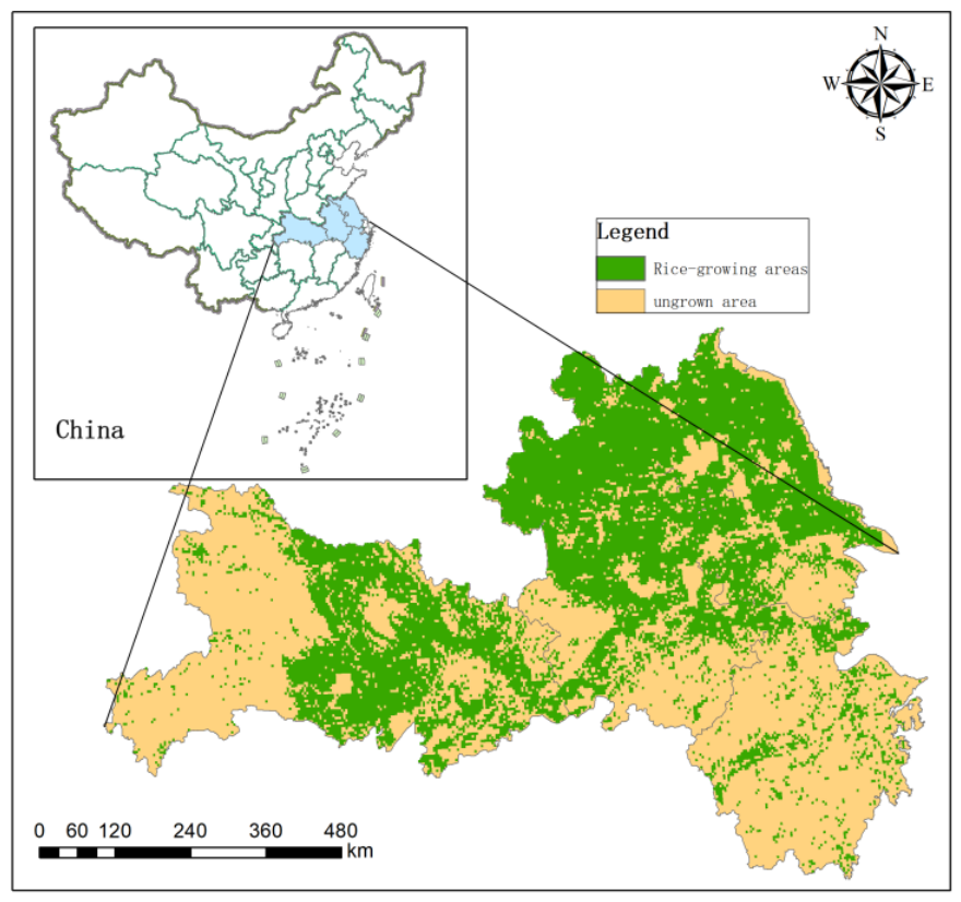
The MLYR is one of the major rice-producing regions in China (Figure 1), accounting for approximately 46% of the total rice cultivation area nationwide. Among them, Hubei, Anhui, Jiangsu, and Zhejiang Provinces are dominated by single-cropping rice cultivation [15]. The growing season of single-cropping rice lasts from June to October, and it is mainly governed by weather systems such as mid–high-latitude atmospheric circulation and the Western Pacific Subtropical High [16]. This climatic background exposes rice to frequent heat damage and causes substantial economic losses. Severe rice heat damage events in this region have drawn attention worldwide.

2.2. Data Source

In this study, multi-source meteorology, remote-sensing, crop, and soil data were used to construct a hazard assessment model of heat damage to single-cropping rice. The main data types and sources are shown in

Table 1. Main data types and sources.

Data Type	Data Content	Data Sources	Spatial Resolution	Time
Meteorological Data	Daily temperature (highest, lowest, average), precipitation, evapotranspiration	The Chinese high-resolution long-term air temperature and precipitation grid dataset (https://doi.org/10.1594/PANGAEA.941329)	1 km × 1 km	1991–2024
Remote Sensing Data	7-day interval VHI data	Global Vegetation Health products https://www.star.nesdis.noaa.gov/smcd/emb/vci/VH/index.php (accessed on 25 August 2026)	4 km × 4 km	1991–2024
	8-day interval GLASS GPP AVHRR data	National Earth System Science Data Center	0.05° × 0.05°	1991–2018
	8 d interval SIF-GPP data	“OCO-2” SIF dataset (GOSIF) https://globalecology.unh.edu/data/GOSIF.html (accessed on 25 August 2026)	0.05° × 0.05°	2000–2024
	Rice planting system	Data set of crop planting system in major countries in the Asian monsoon region https://doi.org/10.6084/m9.figshare.13567526 (accessed on 25 August 2026)	500 m × 500 m	1991–2021
Crop Data	Rice yield data	Statistical Yearbook, Department of Planting Industry Management, Ministry of Agriculture and Rural Affairs, PRC http://www.moa.gov.cn/ (accessed on 25 August 2026)	Provinces, cities, and counties in the MLYR	1991–2024
	Rice growth and development data	The Chinese Academy of Meteorological Sciences	36 agricultural meteorological stations in the MLYR	1991–2024
Soil Data	Daily root-zone soil moisture data	The National Soil Moisture Data Set http://dx.doi.org/10.11888/Terre.tpdc.272415	1 km × 1 km	1991–2024
Miscellaneous Data	Historical disaster data	Disaster grand ceremony, disaster yearbook, Chinese agricultural statistics	Provinces, cities, and counties in the MLYR	1991–2024
	Basic geographic information data	Research Center for Resources and Environmental Sciences, Chinese Academy of Sciences (RESDC) http://www.resdc.cn (accessed on 25 August 2026)	MLYR	1991–2024

. The data were taken from the 1991–2024 time period. Spatial dimension: All raster datasets were aligned to a grid system with 4 km spatial resolution, CGCS2000 coordinate system, and Albers equal-area projection. Detailed data preprocessing procedures are provided in the Supplementary Materials.

2.3. Methods

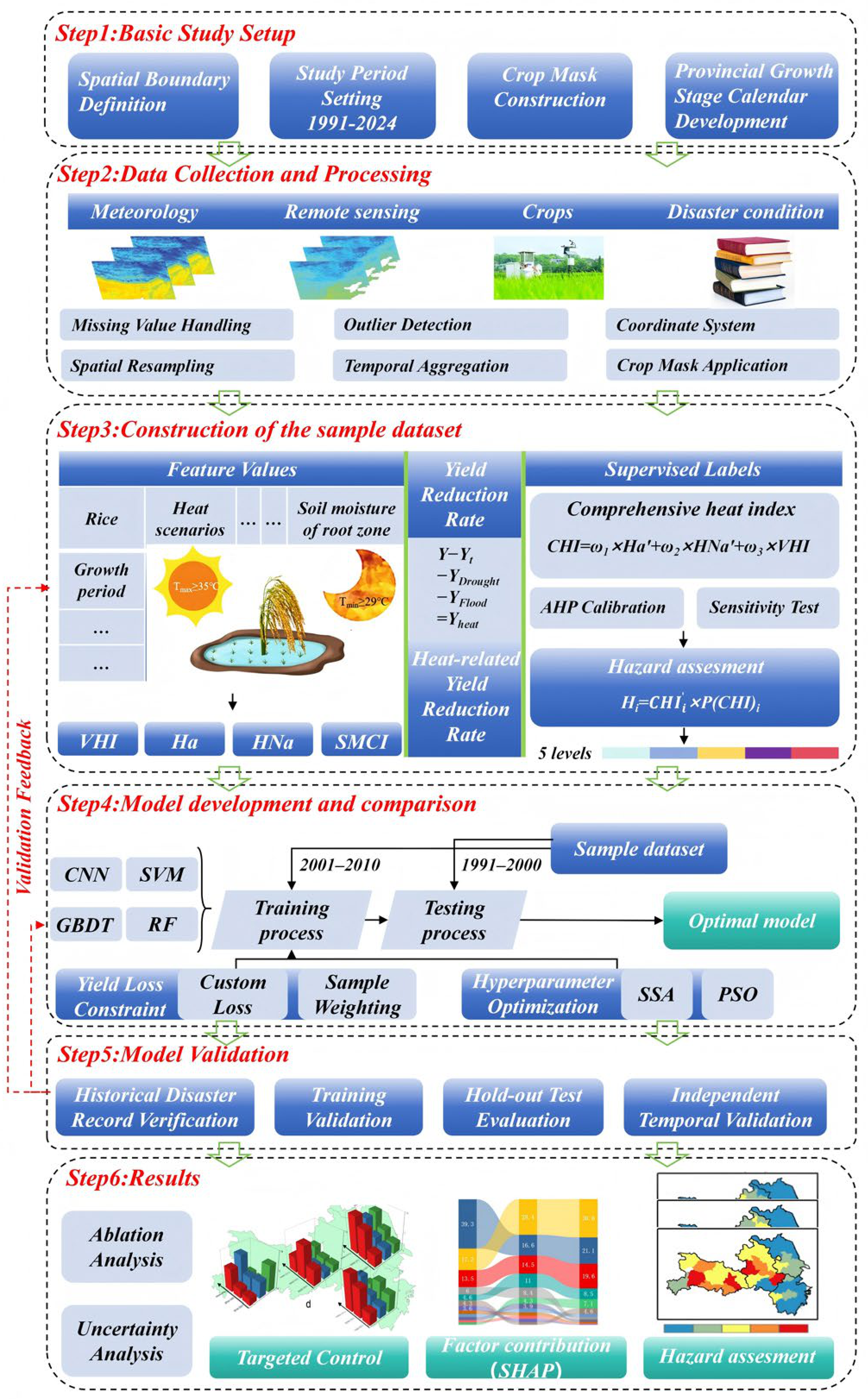
The overall technical workflow of this study is illustrated in Figure 2, with the steps taken detailed as follows: ① Basic setup: Define the spatial boundary and research period, construct a crop mask, and develop a provincial growth stage phenology calendar. ② Data acquisition and preprocessing: Collect multi-source data including meteorology, remote sensing, soil, crop, yield, and historical disaster records and perform missing value handling, outlier detection, coordinate alignment, spatial resampling, temporal aggregation, and crop mask application. ③ Index construction and yield separation: Calculate growth stage–specific core indicators, including daytime and nighttime harmful accumulated temperature, VHI, and root-zone soil moisture. Construct the CHI via AHP calibration, followed by grade definition and a sensitivity test. Conduct yield detrending to extract the heat-related yield reduction rate. ④ Model construction and validation: Divide samples into spatiotemporally independent subsets. Build baseline models with embedded yield constraints and select the optimal model through hyperparameter optimization and multi-model comparison. Implement multi-dimensional validation, including in-training validation, hold-out test evaluation, independent temporal validation, and historical disaster record comparison. ⑤ Result interpretation: Conduct uncertainty analysis and ablation analysis, interpret driving mechanisms using the SHAP method, map the hazard distribution, and propose region-specific prevention and control recommendations. A feedback loop is established in the validation phase: identified inconsistencies are fed back to upstream steps to revise data processing, index construction, or model parameters.

2.3.1. Construction of the Composite Heat Damage Index (CHI)

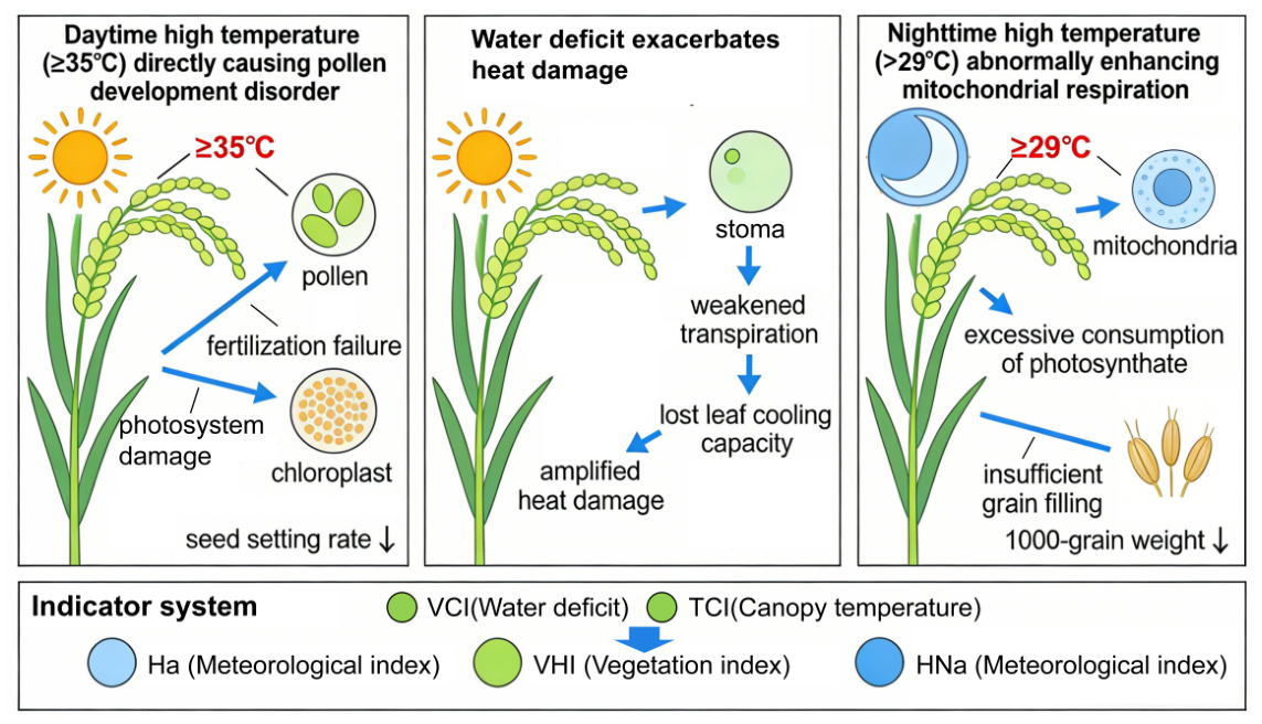
High daytime temperatures reduce the seed-setting rate and grain weight primarily by disrupting pollen development and pollination, inhibiting photosynthesis, and shortening the growth period. High nighttime temperatures mainly intensify respiratory consumption, disturb grain filling and hormone balance, and generally exhibit higher sensitivity to yield loss. Various studies have documented that rice exposed to high nighttime temperatures of 29 °C (33/29 °C, day/night) during the reproductive growth stage experiences carbon deficit in photosynthates driven by intensified respiratory metabolism, resulting in notable yield loss [17]. Importantly, the damage induced by high nighttime temperatures is characterized by sudden onset and pronounced detrimental effects, as even a single day of short-term exposure can significantly reduce spikelet fertility and grain weight [18]. Water deficit induces stomatal closure and suppresses transpiration, which impairs the heat dissipation capacity of plants and exerts an amplifying effect on heat damage (Figure 3) [19]. Due to the interaction of multiple factors, the occurrence of rice heat damage is highly complex and variable; therefore, monitoring based on a single meteorological index cannot fully reflect the actual conditions of heat damage.

Accordingly, the harmful accumulated temperature (Ha) [20] is selected as the daytime heat damage index. Following the same formulation as Ha, the nighttime harmful accumulated temperature (HNa) is constructed as the nighttime heat damage index, and the Vegetation Health Index (VHI) is further introduced. The VHI is composed of the Vegetation Condition Index (VCI) and the Temperature Condition Index (TCI) [21]. The VCI reflects actual vegetation growth status and the exacerbating effect of water deficit on heat damage, while the TCI captures canopy temperature variations to more accurately identify high-temperature stress and prevent the VCI from over-amplifying the effect of water deficit.

Furthermore, heat damage involves complex interactions within the soil–crop–atmosphere continuum system [22]. Based on remote sensing canopy observations, the VHI accounts for the deviation between air temperature and rice canopy temperature, accurately characterizing the transpiration capacity of single-cropping rice during critical growth stages. It also integrates underlying surface information missing from traditional meteorological indices, endowing the comprehensive index with a precise hazard-identification capabilities.

Meteorological data obtained from the National Meteorological Information Center were used to calculate the HNa and Ha, while the VHI was calculated from the NDVI retrieved using remote sensing. All three indices are on a weekly scale. Finally, the comprehensive heat damage index (CHI) was constructed using the analytic hierarchy process (AHP) implemented in Python (version 3.9.0, Python Software Foundation, Wilmington, DE, USA) [23], calculated as follows:

$${CHI}_i={\omega }_1\times {{Ha}_i}^{\prime }+{\omega }_2\times {{HNa}_i}^{\prime }+{\omega }_3\times {VHI}_i$$

(1)

where ${{Ha}_i}^{\prime }$ and ${{HNa}_i}^{\prime }$ denote standardized indicators; and ${\mathsf{\omega }}_1$, ${\mathsf{\omega }}_2$, and ${\mathsf{\omega }}_3$ are the indicator weights determined by the AHP, with values of 0.501, 0.169, and 0.330, respectively.

Both the HNa and Ha are positive indicators of hazard intensity, whereas the VHI is a negative indicator of hazard risk. Accordingly, the HNa and Ha were converted to negative indicators via min–max normalization, with all values scaled to the interval [0, 1]. The resulting CHI functions as a negative indicator, where higher CHI values correspond to healthier rice status or milder heat damage. The grading thresholds for the VCI and VHI were determined with reference to the meteorological grades of rice heat damage, the Technical Specification for Remote Sensing Monitoring and Assessment of Flood and Drought Disasters (SL750-2017, Water Conservancy Industry Standard of the People’s Republic of China), and relevant studies. As the CHI is calculated as the weighted average of three indicators, its stress grading criteria were formulated by referencing the three indices and revised against disaster records from 1991 to 2000 (

Table 2. Classification of rice heat damage grades based on the CHI.

Heat Damage Grade	CHI
Normal	(0.75, 1]
Light	(0.65, 0.75]
Moderate	(0.55, 0.65]
Severe	(0, 0.55]

).

The scientific rationale for weight assignment (Tables S3–S6) [18,24,25], sensitivity analysis (Tables S7 and S8), and detailed calculation methodologies for indicators, including Ha (Equations (S1)–(S3) and Tables S1 and S2), are available in the Supplementary Materials.

(1)

Nighttime harmful accumulated temperature (HNa)

High nighttime temperatures experienced during heat events increase the risk of heat damage to rice yield. Simulating the harmful accumulated temperature, the 95th percentile of the normal distribution of minimum temperature series from July to September in the MLYR from 1991 to 2024 (i.e., ≥29 °C) was taken as the rice high-nighttime-temperature threshold:

$$HNa={\displaystyle \sum _{j=1}^m}{\displaystyle \sum _{i=1}^{n_j}}\left[\mathit{f}\left(T_{\mathit{L}}^{ij}\right)\right]$$

(2)

$$f\left(T_L^{ij}\right)=T_L^{ij} - 29.0 T_L^{ij} \ge 29.0$$

(3)

where HNa is the nighttime harmful accumulated temperature, in degree-days (°C·d); m is the total number of rice heat damage processes during the evaluation period; j is the serial number of multiple rice heat damage processes, j = 1, 2, 3, …, m; ${\mathrm{n}}_{\mathrm{j}}$ is the total number of high-temperature days in the j-th rice heat damage process, in days (d); i is the serial number of each day in the j-th rice heat damage process, i = 1, 2, 3, …, n; $\mathrm{f}\left({\mathrm{T}}_{\mathrm{L}}^{\mathrm{ij}}\right)$ is the single-night accumulated heat; and ${\mathrm{T}}_{\mathrm{L}}^{\mathrm{ij}}$ is the daily minimum temperature on the i-th day of the j-th rice heat damage process.

2.3.2. Definition of Multi-Scenario Rice Heat Damage and Growth Stage Demarcation

(1)

If high-temperature days (maximum temperature > 35 °C) occur for three or more consecutive days in a given week, daytime heat damage is considered to have occurred in that growth stage. If high nighttime temperature days (minimum temperature > 29 °C) occur for no less than 1 day in a given week, nighttime heat damage is considered to have occurred in that week. Processes are counted per growing season (year), not across years. If daytime heat damage occurs in a given week and water deficit is identified by the VHI in that week, water deficit–affected heat damage is considered to have occurred in that week.

(2)

Heat damage for single-cropping rice in the MLYR is concentrated in July–August after the plum rain season, when single-cropping rice is in the booting, heading–flowering, and grain-filling stages and is prone to sustained high-temperature weather controlled by the Western Pacific Subtropical High and mid-latitude atmospheric circulation systems [26]. Therefore, the booting, heading–flowering, and grain-filling stages were selected as key growth stages (

Table 3. Key growth stages of single-cropping rice.

Province	Booting Stage (Week)	Heading Stage (Week)	Grain-Filling Stage (Week)
Hubei	30–31	32–33	34–35
Anhui	30–32	32–34	35–36
Jiangsu	32–33	34–35	36–37
Zhejiang	32–34	35–36	37–38

).

2.3.3. Estimation of Heat-Associated Yield Anomaly

The MLYR is a region with frequent meteorological disasters. Yield reduction in single-cropping rice is mainly affected by three types of disaster, namely drought, flood, and heat, and the dominant meteorological disaster type varies each year. Therefore, when conducting heat damage risk analysis, the heat-associated component of the yield anomaly must be separated. However, heat damage in the MLYR generally occurs concurrently with other disasters, resulting in insufficient samples to accurately model the relationship between meteorological heat damage indices and yield reduction alone. Therefore, we first established a model of meteorological disasters and yield reduction rates in non-heat years. We then estimated heat-associated yield anomalies in heat years as the residual after accounting for drought and flood effects. Detailed separation methods and illustrative examples, together with Equations (S4)–(S7), Tables S9–S11, and Figure S1, are provided in the Supplementary Materials.

2.3.4. Construction of Rice Heat Hazard Assessment Model

(1)

Traditional hazard assessment model

Hazard is a function of heat damage intensity and its occurrence frequency [27]:

$$H_i={CHI}_i^{\prime }\times P\left({CHI}_i\right)$$

(4)

$${CHI}_i^{\prime }={1-CHI}_i$$

(5)

where $H_i$ is the heat hazard value, ${CHI}_i^{\prime }$ is heat damage intensity, $P\left({CHI}_i\right)$ is the annual occurrence frequency of heat damage calculated from annual heat weekly frequency, and i is a grid point. The hazard levels were divided into five categories using the Jenks natural breaks method: very high, high, medium, low, and none. Annual hazard is computed per year: each of the 6 critical weeks is graded by the CHI, “none” weeks are excluded, and the within-grade mean positive intensity ${CHI}_i^{\prime }$ is multiplied by that grade’s week proportion and summed across grades. Period-level values are multi-year averages of annual values.

(2)

Machine learning–optimized hazard assessment model

Machine learning algorithms replace the subjective and cumbersome weighting process in traditional methods and can accurately capture nonlinear relationships and interaction effects between features, making the evaluation results more objective and classification more accurate. To prevent machine learning simulation results from merely fitting the outputs of traditional hazard assessment and reduce reliance on conventional labels, yield constraints were introduced to correct deviations caused by subjective weighting.

First, outlier removal and standardization were applied to the raw heat damage factors and yield data, based on which two sets of sample datasets were established. A temporal independent splitting strategy was adopted to partition the full dataset into training and test sets, and an independent validation set was further extracted from the training set by year for hyperparameter tuning and early stopping control. A machine learning heat hazard assessment model embedded with yield constraints was constructed. Multi-class cross-entropy was used as the primary loss function to guide weight optimization and ensure the model’s fitting accuracy for traditional hazard grading. Meanwhile, a yield correlation constraint term was introduced as auxiliary loss, which penalizes samples with mismatched hazard ranking and actual yield reduction ranking, thus improving the consistency between the assessment results and the spatial pattern of actual disaster losses. During training, hyperparameter optimization was performed based on the comprehensive performance of the validation set, and the optimal parameter combination was determined as the final model configuration. After model training, generalization performance was evaluated on the independent test set.

(a)

Construction of Sample Datasets

Two types of sample datasets were constructed to support model training and accuracy validation respectively:

County-year calibration dataset: Used for yield constraint calibration during the training phase. Taking counties as statistical units, we matched county-level yield reduction rates from 1991 to 2024 with the regional averages of the VHI, Ha, HNa, and soil moisture across growth stages within each corresponding county (

Table 4. Hazard evaluation indicator system.

Growth Stage	Scenario Type	Indicator (Feature Value)
Booting stage (BS) Heading stage (HS) Grain-filling stage (GFS)	Daytime heat damage (RDHH)	Harmful accumulated temperature (Ha)
	Nighttime heat damage (RNHH)	Nighttime harmful accumulated temperature (HNa)
	Water deficit–affected heat damage (RHH&D)	Vegetation Health Index (VHI)
	Hazard-forming environment	Root-zone soil moisture (SMCI)

). A total of 150 counties with a data missing rate below 5% were selected as the study sample set. Missing values for specific years were imputed via trend interpolation using data from adjacent counties in the same period, and only intra-period data were used in the imputation process to avoid introducing future information. Finally, 5009 valid county-year calibration units were obtained.

Grid feature dataset: Used for model feature input and hazard grading output. Taking 4 km grids as the minimum unit, the dataset contains 12 features including the VHI, Ha, HNa, and soil moisture for each growth stage per grid, as well as 5-level hazard grading labels calculated based on the traditional CHI, which serve as the supervised classification benchmark for the model.

(b)

Partition of Training and Test Sets

The 1991–2000 period was selected as the training period, and the 2001–2010 period was selected as the independent test period. Since 2001–2010 and 2011–2020 both fall within the accelerating phase of climate warming, the interannual climatic features exhibit strong temporal autocorrelation, posing a risk of trend leakage [28,29,30]. By contrast, the 1991–2000 period represents the early stage of climate warming, with significantly lower overall heat hazard intensity than the test period and greater differences in disaster distribution characteristics. Furthermore, heat hazard assessment models need to ensure rational grading across the full intensity range. Samples from 2001 to 2010 and 2011 to 2020 are concentrated in the medium–high disaster intensity range, which easily leads to a blind zone where the model produces distorted grading for low-intensity hazards.

Training set: The 1991–2000 period was selected as the training period. Each sample contains 12 factor features and CHI hazard grading labels. County-year yield reduction rates were only used to calculate the yield constraint loss term, not directly as input features of the model. An independent validation set was split from the training period along the temporal dimension [31], which did not participate in weight updates and was only used for early stopping control and hyperparameter performance validation during training (

Table 5. Dataset partitioning.

Modeling Phase	Time Range	Number of Counties	County-Year Units	Number of Grid Samples
Yield constraint estimation subset	1991–2000	100	1000	Aggregated at the county level
Model training set	1991–1998	100	800	8000 (1000 grids per year)
Hyperparameter validation set	1999–2000	100	200	2000 (1000 grids per year)
Independent test set	2001–2010	150	1500	All rice-growing grids within the study area
Generalization set	2011–2024	150	2081	All rice-growing grids within the study area
Full archive	1991–2024	150	5009	All rice-growing grids within the study area

) [32].

(c)

Model input variables and supervised labels

These variables and labels comprise the 12 feature values, including multi-scenario hazard and disaster-pregnant environment impacts, in the hazard evaluation indicator system in Table 4. The VHI was standardized as a positive indicator to align its polarity with that of the Ha and HNa. All four indices were calculated from a weekly scale to a growth-stage scale. Finally, the four indices were standardized, with the VHI converted to a positive indicator through standardization.

To ensure that the final hazard conforms to the definition of “intensity × frequency,” hazard assessment results from 1991 to 2000 calculated using the traditional heat hazard assessment model were divided into 5 levels, and the hazard grades were used as supervised labels for the machine learning model.

(d)

Machine learning model construction

Considering data volume and machine learning interpretability, four models were selected: a deep learning CNN model, two basic decision tree models—a random forest (RF) [33] model focusing on stability and a gradient boosting decision tree (GBDT) model focusing on accuracy—and a non-decision tree model support vector machine (SVM) model [33]. Optimization algorithms adapted to each model were selected. Detailed methodological descriptions are provided in the Supplementary Materials (Equations (S8)–(S15)).

(e)

Yield constraint penalty module

The model adopts a custom multi-class objective function embedded with the physical constraints of yield loss. The total loss is composed of a multi-class cross-entropy main loss and a weighted yield correlation constraint term, defined as follows [34,35]:

L_total = L_ce + λ·L_yield

(6)

where λ is the yield constraint weight coefficient, set to 0.2, as determined via grid search, to balance the fitting accuracy of traditional labels against the calibration intensity of actual disaster losses. The determination of the values of parameters λ and α, along with their sensitivity analysis, is fully detailed in the Supplementary Materials (Tables S16 and S17).

Constraint module for CNN and GBDT

Multi-class cross-entropy: The main loss takes the 5-level hazard grades of the comprehensive heat damage index (CHI) classified using the Jenks natural breaks method as sample-wise supervised labels to anchor the core classification framework and disaster-causing logic of traditional hazard assessment. The calculation formula is given as follows:

L_ce = −1/N ∑_{i = 1}^N ∑_{c = 1}⁵ y_i,c log(p_i,c)

(7)

where N is the total number of raster samples in the training set; y_i,c is the one-hot encoding of the true label for the i-th sample; and p_i,c is the predicted probability that the i-th sample belongs to the c-th hazard level output by the model via the Softmax layer.

Yield correlation constraint term: Taking the county-level detrended meteorological yield reduction rate as the independent calibration benchmark, only the relative ranking consistency between hazard and disaster loss is constrained, rather than fitting the absolute value of the yield reduction rate, to avoid deviating from the relative classification attribute of heat hazard. First, the five types of discrete prediction probabilities for each raster sample are weighted and summed according to hazard levels to convert into continuous hazard scores; then, the arithmetic mean is calculated by taking county-year as the statistical unit to obtain county-level average predicted hazard values, which are matched with the yield reduction rate data of the corresponding unit. Finally, after Z-score standardization of the two series, the mean squared error is used as the constraint loss, which is expressed as follows:

L_yield = 1/K ∑_{k = 1}^K [(H_k − μ_H)/σ_H − (Y_k − μ_Y)/σ_Y]²

(8)

where K is the total number of county-year units in the training set; H_k and Y_k are the average predicted hazard and detrended meteorological yield reduction rate of the k-th unit, respectively; and μ_H, σ_H and μ_Y, σ_Y are the mean and standard deviation of the predicted hazard and yield reduction rate series in the training set, respectively.

Adaptive Constraint Implementation for the GBDT Model (XGBoost Custom Objective)

The yield constraint loss defined above is formulated at the county-year aggregated unit scale and cannot be directly applied to sample-wise tree boosting in XGBoost. To address this, a custom objective function was developed based on the XGBoost framework [36]. Using chain rule differentiation, unit-level constraint errors are backward-decomposed and assigned to individual grid samples, enabling joint iterative optimization of classification supervision and yield constraints. XGBoost guides tree node splitting and leaf weight updates using the first-order gradient and second-order Hessian of the loss function with respect to the model’s logit outputs.

The gradient $g_{\mathrm{ce},i,c}$ and Hessian ${\mathrm{h}}_{\mathrm{ce},i,c}$ of the multi-class cross-entropy loss are calculated as follows:

$$g_{\mathrm{ce},i,c} ={ p}_{i,c} -y_{i,c}$$

(9)

$${\mathrm{h}}_{\mathrm{ce},i,c}={ p}_{i,c}\cdot \left(1 - p_{i,c}\right)$$

(10)

where $p_{i,c}$ is the predicted probability that the i-th grid sample belongs to the c-th heat damage grade; and $y_{i,c}$ is the one-hot encoded label of the sample’s actual disaster grade, taking a value of 1 for the true grade and 0 otherwise.

To embed county-level constraint loss into sample-wise optimization, a continuous mean hazard value for each county-year unit was first constructed:

$$H_k={\displaystyle \frac{1}{m_k}}\sum _{i\in k} {\displaystyle \sum _{c=1}^5} w_c\cdot p_{i,c}$$

(11)

where $m_k$ is the number of grid samples contained in the k-th county-year unit; $w_c$ denotes the weight of each heat damage grade, with values 1, 2, 3, 4, and 5 assigned to hazard grades I–V, respectively, to map discrete grading results into continuous hazard values; and i ∈ k represents all grid samples corresponding to the k-th county-year unit.

The gradient of the constraint loss with respect to the logit of class c for sample i is given by the following equation:

$$g_{yield ,i,c}={\displaystyle \frac{2\lambda }{K\cdot {\sigma }_H\cdot m_k}}\cdot \left({\displaystyle \frac{H_k-{\mu }_H}{{\sigma }_H}}-{\displaystyle \frac{Y_k - {\mu }_Y}{{\sigma }_Y}}\right)\cdot w_c\cdot p_{i,c}\cdot \left(1 - p_{i,c}\right)$$

(12)

where $p_{i,c}\cdot \left(1-p_{i,c}\right)$ is the chain rule derivative term of the Softmax output with respect to the logit. The second derivative of the constraint term exhibits large numerical fluctuations; to ensure training stability, the Hessian of the total loss retains the second-order term from the cross-entropy loss.

Constraint integration mechanism: During training, gradients from the county-level yield constraint loss are decomposed to each grid sample and fused with classification gradients to jointly guide XGBoost tree structure splitting and weight updates, realizing joint constrained optimization of traditional grading supervision and empirical consistency between hazard grading and independent yield anomaly.

Constraint module for RF and SVM

RF and SVM have no globally differentiable loss function or backpropagation chain. Therefore, the sample weight allocation method is adopted, taking county-year as the statistical unit, where the unit weights are calculated according to the relative intensity of the detrended meteorological yield reduction rate within the unit. Then, the unit weights are evenly distributed to all raster samples within the unit so that samples with more severe yield reduction contribute higher weights in decision tree node splitting, guiding the model to strengthen the learning of real disaster-driving features while fitting CHI classification labels. The unit weight calculation formula is given as follows:

W_k = 1 + α·(Y_k − μ_Y)/σ_Y

(13)

where W_k is the weight coefficient of the k-th county-year unit; Y_k is the detrended meteorological yield reduction rate of the corresponding unit; μ_Y and σ_Y are the mean and standard deviation of the yield reduction rate in the training set, respectively; and α is the constraint strength coefficient, set to 0.2. The controlled variable principle was adopted, where the strength of the constraint module was set as a uniform control variable with a fixed value of 0.2, matching the constraint strength of the other models. To ensure non-negative weights, weights below 0 are truncated to 0.

The final training weight for the i-th raster sample is defined as follows:

w_i = W_k/M_k, i ∈ S_k

(14)

where S_k is the set of raster samples contained in the k-th county-year unit, and M_k is the number of raster samples in the unit.

2.3.5. Ablation Study

To quantify the incremental value of each methodological component, identify the core sources of contribution [37], and determine whether the primary improvement stems from the novel CHI, yield constraints, GBDT flexibility, or the optimization procedure, two sets of experiments were designed in this study: progressive ablation and single-component leave-one-out ablation. Progressive ablation design: the traditional Ha-based heat hazard assessment (A0) was compared with the CHI-based heat hazard assessment (A1), and the machine learning model trained with unconstrained CHI labels (A2) was compared with the proposed yield-constrained machine learning model (A3). Single-component leave-one-out ablation: the effects of individual components were excluded one by one, including the high nighttime temperature variable (B1), VHI (B2), growth stage information (B3), and clustered hyperparameter optimization (B4).

Performance variations were evaluated in terms of balanced accuracy, macro-F1 score, multi-class AUC, yield correlation, calibration error, spatial consistency, and consistency with historical records.

2.3.6. SHAP Algorithm

The SHAP (Shapley additive explanations) algorithm is an additive feature attribution method used to interpret the outputs of machine learning models, rooted in game theory. It is used to determine the contribution of each feature to the model output. SHAP has two unique advantages: first, it supports both global and local interpretation; second, SHAP interaction values ensure consistency in the interpretation of feature interaction effects. Compared to existing feature importance metrics in machine learning models, SHAP has advantages in terms of identifying whether the contribution of each input feature is positive or negative. In addition, each observation has a corresponding SHAP value, so SHAP can help interpret both global and local model behavior [38].

$$y_i=y_{base}+f\left(x_{i1}\right)+f\left(x_{i2}\right)+\dots +f\left(x_{ij}\right)$$

(15)

where $y_{\mathrm{base} }$ is the mean value of the target variable across all samples, and $f\left(x_{ij}\right)$ is the SHAP value of feature $x_{ij}$.The implementation of the SHAP method is detailed in the Supplementary Materials (Equations (S16) and (S17)).

3. Results

3.1. Spatiotemporal Variation Characteristics of Multi-Scenario Heat Damage in Single-Cropping Rice

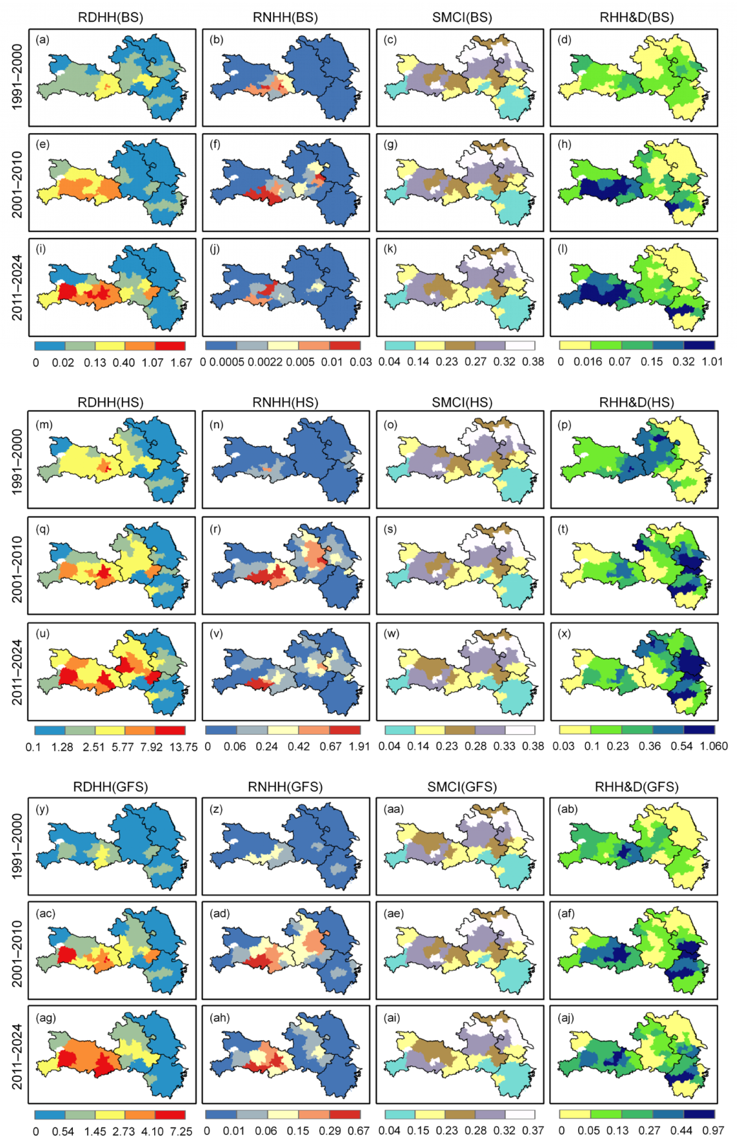
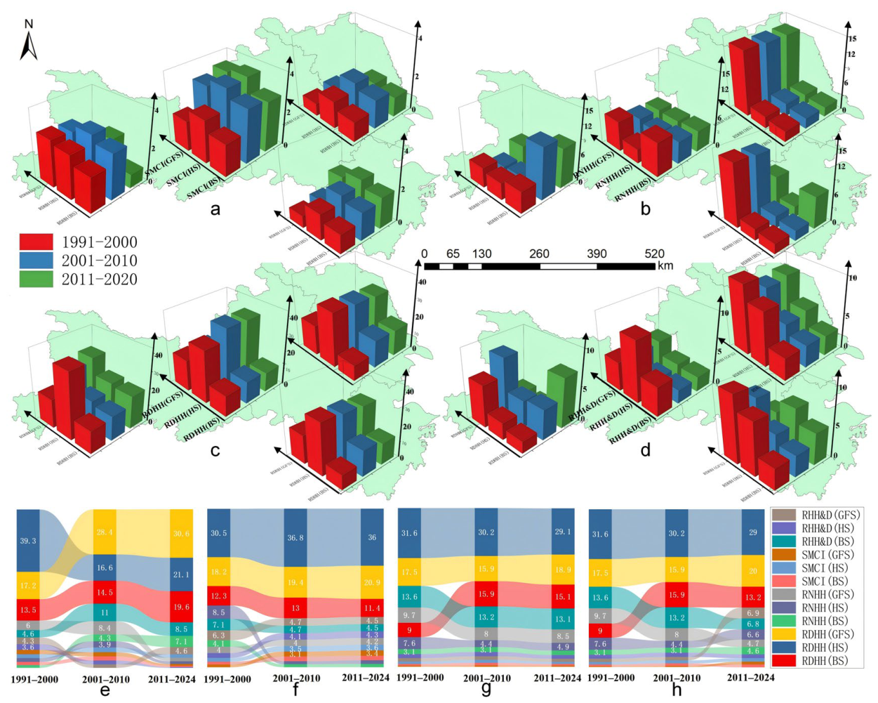
The intensity of daytime heat damage to single-cropping rice exhibited an increasing trend every decade (Figure 4). The intensity of nighttime heat damage rose from 1991 to 2000, and then from 2001 to 2010, before declining in 2011–2024. Hubei Province suffered severe nighttime heat damage throughout rice growth stages, while Jiangsu and Zhejiang Provinces only experienced mild nighttime heat damage at the heading stage. Water deficit–affected heat damage showed a continuous upward trend over the 30-year period, reflecting the frequent occurrence of combined drought–heat events. Hubei Province recorded the highest severity of water deficit–affected heat damage at the booting stage of single-cropping rice. No obvious long-term trend was observed in root-zone soil moisture over the three decades, and the average root-zone soil moisture during the grain-filling stage was lower than that during the booting and heading–flowering stages.

3.2. Rationality Validation of CHI and Hazard Assessment Results

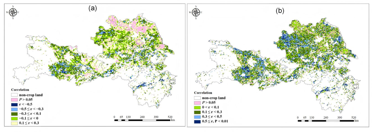
GPP data were used to examine the correlations between the Ha and the newly developed index with vegetation productivity (Figure 5).

From 1990 to 2024, the correlation coefficient between the cumulative GPP and CHI across critical SCR growth stages ranged from 0 to 0.78. Although the GPP was also affected by other disasters occurring from January to August, the average correlation coefficient still reached 0.55, confirming the significant impact of rice heat damage on the GPP. The average correlation between the Ha and GPP was 0.36, and the average correlation between the GPP and the composite index was significantly higher than that of the Ha. Correlation analyses were conducted between yield reduction rates and hazard values derived from the Ha and CHI, respectively, with all passing the significance test at p < 0.05. Details are provided in the ablation experiments presented in Section 3.4.

3.3. Performance Comparison and Model Validation of Yield-Constrained Machine Learning Models

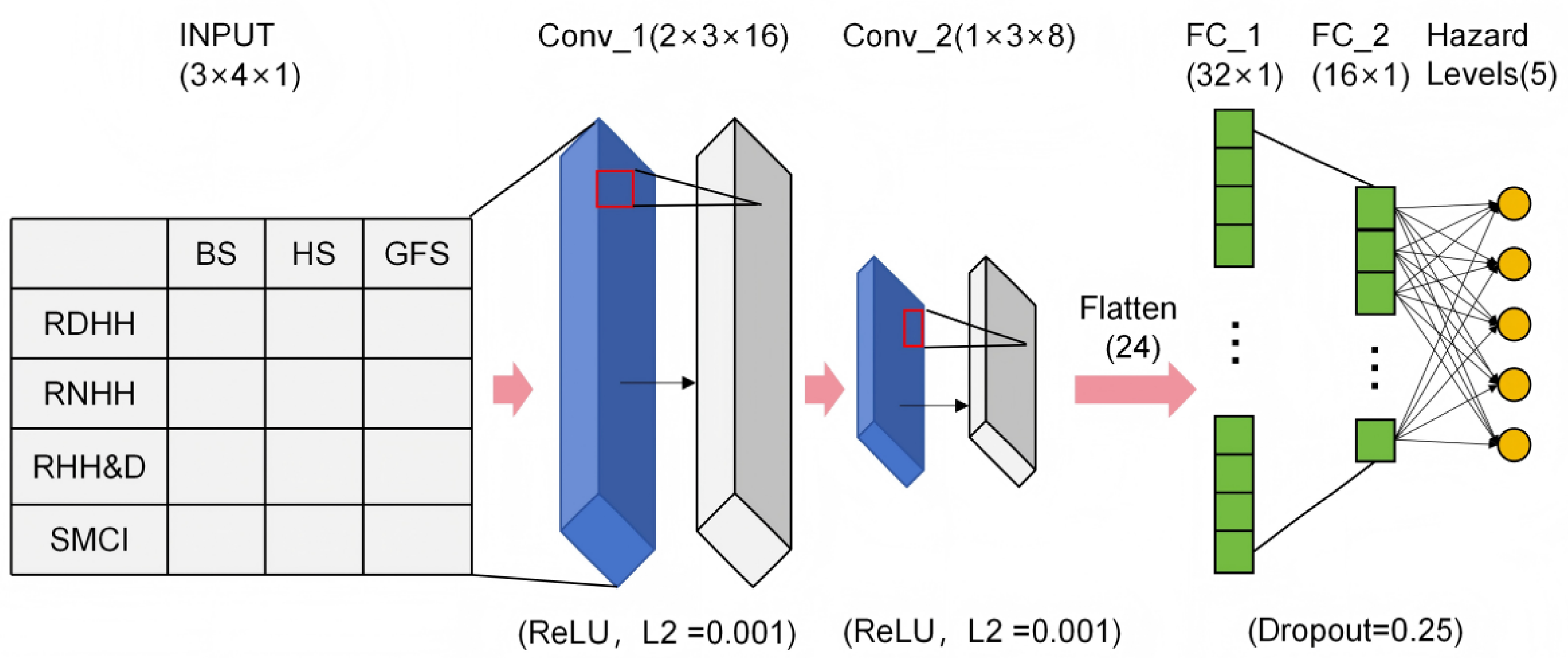
Model performance was determined via optimization strategies, which covered parameter tuning, data preprocessing, and other approaches. For the CNN model, the numbers of neurons and convolutional kernels were selected to adapt to the small sample size, prevent overfitting, and balance generalization capacity.

In the architecture shown in Figure 6, INPUT denotes the input layer, restructured into a two-dimensional layout following the logic of growth stages (three categories) × factor types (four categories). Conv_1 is the first convolutional layer, designed to extract two-dimensional local correlation features of adjacent factors within the same growth stage and the same factor across adjacent growth stages. Conv_2 is the second convolutional layer, which further extracts interactive pattern features across multiple growth stages and multiple factors based on the local features extracted by Conv_1. Subsequently, a flattening module converts the three-dimensional feature maps into one-dimensional vectors, realizing global feature fusion via local feature extraction. FC_1 and FC_2 are fully connected layers that perform secondary dimensionality reduction and refinement on the global features, producing the final five-class hazard classification results. Detailed construction parameters are provided in the Supplementary Materials (Tables S12 and S13).

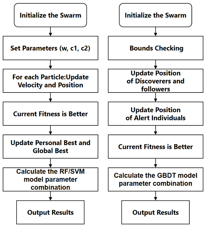
In this study, particle swarm optimization (PSO) was applied for hyperparameter optimization of RF and SVM (Figure 7). The main parameters of the PSO algorithm were set as follows: swarm size = 10; maximum iterations = 10. The sparrow search algorithm (SSA) was adopted for hyperparameter optimization of GBDT, with the main parameters set as follows: population size = 20; maximum iterations = 50; safety threshold = 0.8; proportion of discoverers = 20%; and proportion of alert individuals = 10%. The optimized main hyperparameter values of the models are provided in the Supplementary Materials (Tables S14 and S15).

The accuracy test results of each model on the test dataset are summarized in

Table 6. Accuracy of each model.

Model	SVM	RF	CNN	GBDT
Overall accuracy (%)	83.0 ± 1.7	87.0 ± 0.8	90.0 ± 1.3	94.0 ± 1.0
Balanced accuracy (%)	79.6 ± 2.0	84.1 ± 1.0	87.3 ± 1.5	92.6 ± 1.2
Macro F1 score	0.771 ± 0.020	0.825 ± 0.010	0.862 ± 0.015	0.918 ± 0.012
Weighted F1 score	0.827 ± 0.018	0.869 ± 0.009	0.898 ± 0.013	0.947 ± 0.010
Cohen’s Kappa	0.758 ± 0.022	0.826 ± 0.011	0.864 ± 0.016	0.932 ± 0.013
MCC coefficient	0.718 ± 0.024	0.785 ± 0.012	0.829 ± 0.017	0.901 ± 0.014
Macro-average AUC (one vs. rest)	0.909 ± 0.014	0.922 ± 0.007	0.953 ± 0.011	0.967 ± 0.008
ROC	0.9094	0.9222	0.9526	0.9668

. The results show that model performance ranked in the order of GBDT > CNN > RF > SVM. After optimization via the sparrow search algorithm, the GBDT model achieved an overall accuracy of 94%.

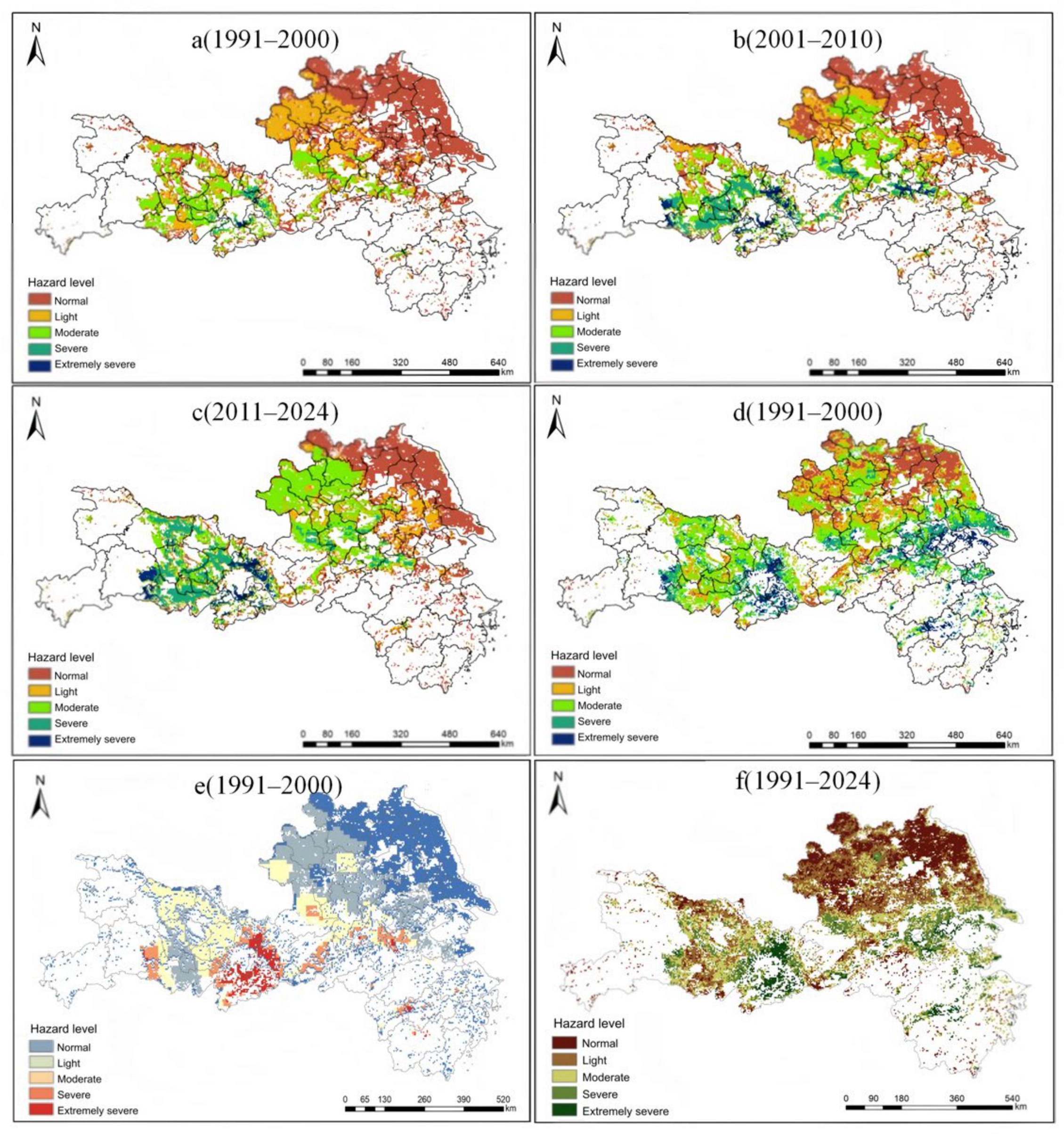
Figure 8e presents the CHI heat hazard assessment results calculated using the traditional model, while Figure 8d shows the results derived from the CNN model (Figure 8). The hazard levels in Anhui and Hubei Provinces derived from the CNN model were generally consistent with those obtained from the GBDT model, whereas the hazard values estimated using the CNN model in southern Jiangsu and Zhejiang Provinces were significantly higher than the GBDT results. A comparison with the remote sensing index, the VHI (panels i, x, and aj in Figure 4), revealed that the CNN model outputs aligned more closely with the VHI. Limited by the sample size, the CNN model may over-extract the dual stress features of water deficit and high temperatures during feature learning, causing water deficit–affected heat damage (RHH&D) to dominate the hazard assessment over daytime heat damage (RDHH). This mechanism also explains the relatively lower ROC value of the CNN model. Additional systematic evaluations were conducted using the GBDT model, covering classification performance assessment, spatial transferability validation, and generalization experiments. The comprehensive results are fully documented in the Supplementary Materials (Tables S18–S27 and Figures S2 and S3). Accordingly, it can be concluded that the GBDT model is the most suitable approach for heat hazard assessment of single-cropping rice. It not only possesses the strongest capability to capture heat damage features but also yields feature patterns that best conform to actual field conditions.

3.4. Progressive and Single-Component Ablation Experiments

To clarify the incremental value of each methodological component and identify the core sources of contribution, two sets of experiments were designed: progressive ablation and single-component removal ablation. Quantitative evaluations were conducted from the dimensions of classification accuracy, empirical consistency, and spatial consistency, with 95% confidence intervals provided for all performance variations.

The results of progressive ablation verified the rationality of the methodological upgrades. From the single Ha hazard assessment to the CHI multi-scenario integrated evaluation, the yield correlation coefficient increased from 0.52 to 0.63, and the matching rate with historical disaster records rose by 10 percentage points, confirming the necessity of the integrated daytime–nocturnal–vegetation evaluation framework. The GBDT model without yield constraint realized the transformation from linear rules to a nonlinear model carrier, but its yield correlation slightly decreased due to information loss caused by grading discretization. After introducing the physical yield constraint, the model achieved a yield correlation coefficient of 0.70, a historical record consistency of 94.0%, and a 15.3% reduction in expected calibration error at the cost of a minor decrease of 1.1 percentage points in balanced accuracy. This achieved a scientific trade-off between label fitting precision and empirical consistency (

Table 7. Progressive ablation of methodologies.

Scenario No.	A0	A1	A2	A3
Model Scheme	Traditional Ha hazard Model	Traditional CHI Hazard Model	GBDT Model Without Yield Constraint	Full Model
Balanced Accuracy (%)	-	-	93.7 ± 1.2	92.6 ± 1.2
Macro-F1 Score	-	-	0.930 ± 0.014	0.918 ± 0.012
Multi-class AUC (one vs. rest)	-	-	0.975 ± 0.009	0.967 ± 0.008
Yield Correlation (Pearson’s r)	0.52	0.63	0.59 ± 0.03	0.70 ± 0.03
Expected Calibration Error	-	-	0.072 ± 0.008	0.061 ± 0.007
Spatial Consistency (Kappa)	0.79	1.00 (baseline)	0.91 ± 0.02	0.87 ± 0.02
Historical Record Consistency (%)	80	90	87 ± 1.1	94.0 ± 1.0

).

The single-component ablation experiments further clarified the contribution hierarchy of each element. The VHI is the core component of the CHI, and its removal led to the most significant deviation in classification accuracy and spatial pattern. Nocturnal high temperatures have a stronger marginal explanatory power for actual yield loss; their removal caused a larger decline in yield correlation and disaster matching degree, verifying the calibration effect of yield constraint on the bias of traditional AHP weighting. The growth stage–specific feature organization has a limited impact on overall performance, and its core value lies in the fine-grained analysis of driving mechanisms. SSA swarm intelligence hyperparameter optimization delivered a stable accuracy gain of 1.5 percentage points. In summary, the core methodological innovation of this study stems from the coupled design of the CHI multi-scenario evaluation framework and physical yield constraint, while GBDT nonlinear fitting and SSA optimization serve as technical supporting elements rather than core sources of contribution (

Table 8. Single-component ablation.

Scenario No.	A3	B1	B2	B3
Model Scheme	Full Model	VHI Removed	Nocturnal High Temperature (HNa) Removed	Growth Stage–Specific Feature Organization Removed
Balanced Accuracy (%)	92.6 ± 1.2	88.5 ± 1.3	90.3 ± 1.4	91.8 ± 1.2
Macro-F1 Score	0.918 ± 0.012	0.875 ± 0.015	0.891 ± 0.016	0.907 ± 0.013
Multi-class AUC	0.967 ± 0.008	0.947 ± 0.009	0.954 ± 0.010	0.962 ± 0.008
Yield Correlation (Pearson’s r)	0.70 ± 0.03	0.64 ± 0.03	0.62 ± 0.03	0.66 ± 0.03
Expected Calibration Error (ECE)	0.061 ± 0.007	0.070 ± 0.008	0.067 ± 0.008	0.065 ± 0.008
Spatial Consistency (Kappa)	0.87 ± 0.02	0.83 ± 0.02	0.85 ± 0.02	0.88 ± 0.02
Historical Record Consistency (%)	94.0 ± 1.0	92.0 ± 1.2	90.8 ± 1.3	93.1 ± 1.1

).

3.5. SHAP-Based Model Interpretation and Analysis

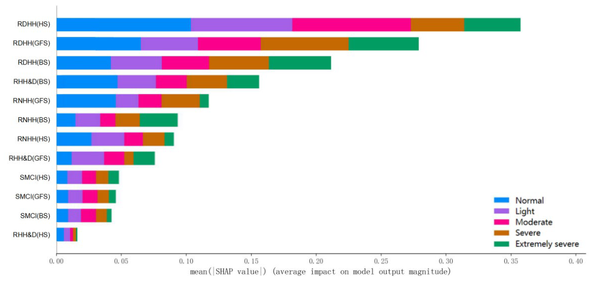
3.5.1. Overall Sample Analysis and Feature Importance Ranking

Over the 34-year period, from the perspective of growth stages, features at the heading–flowering stage exhibited the highest overall relative importance for the model’s hazard grading output, while features at the booting stage showed relatively lower overall importance. In terms of factor types, high daytime temperature–related features had the highest relative importance, followed by high nighttime temperature–related features, with both categories ranking among the top seven in the importance ranking. Notably, the relative importance of the VHI at the booting stage ranked fourth, indicating that the combined drought and heat stress during the booting stage is a non-negligible feature dimension in model grading (Figure 9).

3.5.2. Regional Impact Analysis of Feature Variables

The decadal changes in the absolute SHAP values (contribution degree) of each factor across different growth stages were calculated at the provincial level (Figure 10).

In 1991–2000, the relative importance of high daytime temperatures at the booting stage in Zhejiang and Jiangsu Provinces was relatively low, distinct from other growth stages, due to the lower intensity of high daytime temperatures during this period. In Jiaxing, Zhejiang, the annual average number of days with temperatures ≥ 35 °C at the booting stage was 4.2 in 1991–2000, with no records of more than three consecutive days; this figure increased to 8.7 in 2001–2024, and the probability of consecutive high-temperature events rose by 2.3 times.

High daytime temperature is the core dominant factor for hazard grading, which generates a contribution dilution effect. Despite this dilution effect, the average relative importance of high nighttime temperature features for whole-region model grading still exceeded 20%, making it a non-negligible key stress factor. This dilution mechanism was corroborated by the SHAP results: the accumulated high nighttime temperature of single-cropping rice in 2001–2010 increased significantly compared with 1991–2000, but high daytime temperature stress also increased substantially over the same period, intensifying the dilution effect and reducing the relative contribution of high nighttime temperature by 5%. By contrast, in 2011–2024, the accumulated high nighttime temperature decreased slightly from the previous stage, while the growth rate of high daytime temperature slowed and the dilution effect weakened, leading to a 2% rebound in the relative importance of high nighttime temperature. This temporal variation fully demonstrates that high nighttime temperature features exert a stable and independent discriminative effect in the model grading system, and a single high daytime temperature feature alone cannot achieve complete hazard grade differentiation.

The intensity of high daytime temperature heat damage followed the order of Hubei Province > Anhui Province > Zhejiang Province ≈ Jiangsu Province. For heat damage modified by water deficit in some provinces, the ranking of relative importance in the model was completely opposite to the above order. The importance values of the four provinces fluctuated within 2% of the mean, and the whole-region average maintained a stable contribution share of 16%.

The adequacy of root-zone water had a minor impact (5%) on low-hazard areas but a greater impact (10%) on medium–high-hazard areas such as Hubei and Anhui. The relative importance of root-zone water features at the booting stage was higher than that at other growth stages.

3.5.3. SHAP Prediction Probability Analysis

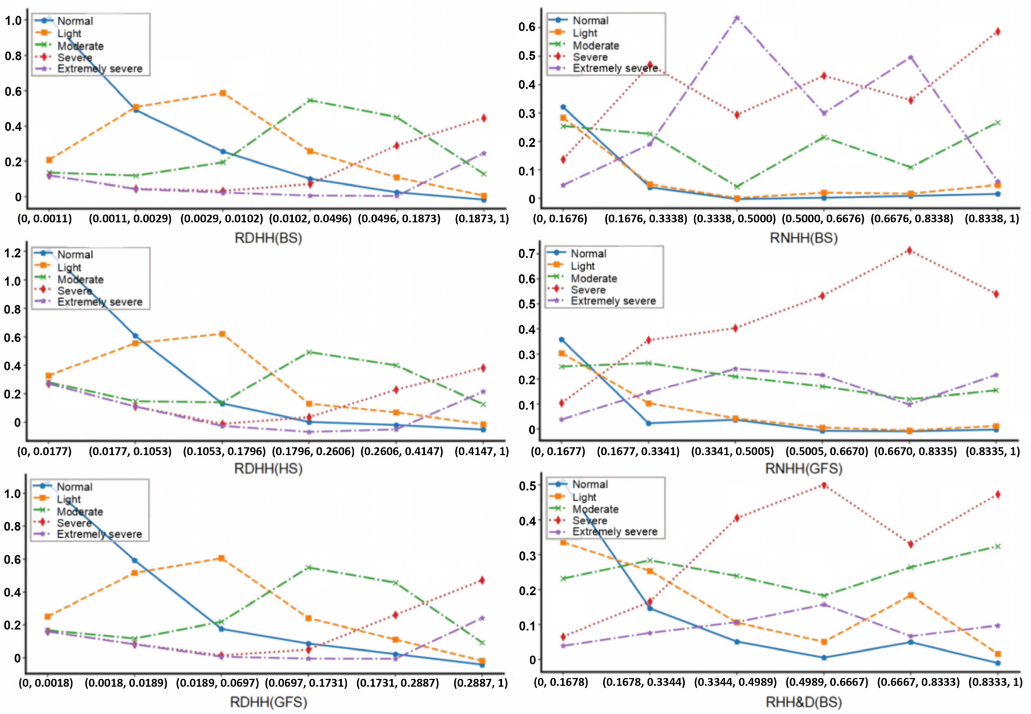
Figure 11 presents the feature contributions calculated via the TreeSHAP method on the logit scale, which were aggregated by feature value binning and mapped to the average predicted probability of each hazard grade. The grade probability changes corresponding to the top six most important features are shown in Figure 11.

As indicated, when the intensity of high daytime temperature heat damage was extremely low, there was an over 80% probability of no hazard. When the intensity approached the median, the probabilities of mild and moderate hazard increased. When high daytime temperature heat damage intensity was high, whether the overall hazard was severe or extremely severe was largely determined by other factors.

When the intensity of high nighttime temperature heat damage at the booting stage exceeded 0.0248, the probability distribution of overall hazard grading covered a wider range, indicating that high nighttime temperature heat damage at the booting stage exhibited strong and distinct sensitivity to hazard grading once it deviated from low values. When the intensity of high nighttime temperature heat damage at the grain-filling stage was non-zero, the hazard was highly likely to be classified as severe.

With increasing intensity of water deficit–modified heat damage, the hazard could only be moderate or severe, with a marked rise in the probability of severe hazard. Combined with the regional difference ranking, this indicates that water deficit can only slightly amplify heat stress intensity on the basis of high daytime temperature and does not possess strong discriminative ability to independently differentiate disaster grades. Compared to the sensitive identification capacity of high nighttime temperature for severe and extremely severe heat damage, the grading discrimination effect of water deficit is significantly weaker.

4. Discussion

In this study, a coupled framework was constructed integrating traditional scaling and machine learning calibration, which retains the mechanistic logic of traditional heat hazard assessment while correcting biases from subjective weight assignment via yield constraints. This section discusses the findings from three perspectives: generalization mechanism, physiological connotation of features, and spatial drivers. The scientific significance and unique value of this study are elaborated upon in light of advances in the field.

4.1. Comparison of Applicability Between GBDT and CNN

The performance of GBDT and CNN in the hazard assessment of rice heat damage was compared in this study. The results demonstrate that GBDT outperforms CNN across multiple evaluation metrics, including overall accuracy and Kappa coefficient. Given the scale and structure of the dataset used in this study—spanning 34 years, with 4 km grid units and 12 input features—we explicitly confirm that GBDT is the most appropriate model for this task. Theoretically, CNN is capable of capturing spatiotemporal interactions, which is appealing for deciphering the multi-scale driving mechanisms of heat damage. Nevertheless, CNN is highly prone to overfitting when the data volume is limited. By contrast, tree-based models possess an inherent inductive bias for medium-scale tabular feature data, rendering them less vulnerable to overfitting and more computationally efficient during training [39]. This indicates that deep learning requires large-scale datasets, whereas tree-based models are generally better suited to data of this magnitude. This finding provides a valuable reference for follow-up research in this field.

4.2. Dual Mechanisms of Yield Constraints in Enhancing Model Generalization

Compared to the unconstrained model, the introduction of yield constraints led to a slight decrease in classification accuracy but a significant improvement in yield correlation and matching degree with historical disaster conditions, and the expected calibration error was reduced by 15.3%. The gain in generalization capacity stems from the synergistic effect of statistical regularization and physiological rationality.

From a statistical perspective, the unconstrained model takes only CHI grading labels as the optimization objective, which is prone to overfitting the linear biases and label noise introduced by AHP subjective weight assignment, limiting its generalization ability for independent disaster loss data. The yield constraint takes county-level detrended yield anomaly values as an independent regularization term, compressing the model’s overfitting space for artificial rules and reducing overconfidence in predictions. This effect aligns with the core findings in the field of physics-informed machine learning [40]. In addition, Zhong et al. found that traditional statistical models such as random forest alone tend to systematically underestimate crop yield reduction under extreme climate conditions [41]. After integrating county-level measured yield data, the model’s fitting accuracy for extreme disaster years and spatial generalization capacity improved notably, which indirectly confirms that introducing field yield observations as model constraints can correct prediction biases from pure feature-based modeling, consistent with the rationale of using yield constraints to correct artificial grading noise in this study.

From a physiological perspective, the AHP weights of the CHI are determined based on literature reviews, which underestimate the actual yield reduction effect of factors such as high nighttime temperature. Anchored by field yield losses, the yield constraint drives the model’s feature weights to align with the physiological response patterns of rice to heat damage, making the assessment results more consistent with disaster-causing mechanisms. Unlike existing crop modeling studies that embed physiological process equations (e.g., photosynthesis and respiration) as hard constraints into regression models [11], macroscopic soft constraints of yield loss at the county scale are adopted in this study. This results in the achievement of empirical calibration without embedding complex process equations, making it more suitable for heat hazard assessment in the MLYR. This design of traditional labels as primary supervision and disaster losses as soft constraints not only retains the methodological continuity of the traditional assessment system but also corrects subjective weight biases, providing a feasible low-cost path for upgrading mature assessment methods with machine learning.

4.3. Physiological Basis for the Differentiated Contribution of High Nighttime Temperature

In this study, it was found that the total importance of high daytime temperature across all samples was higher than that of high nighttime temperature, but high nighttime temperature exhibited more significant discriminative ability for medium–high and extremely high disaster grades, demonstrating low overall contribution but strong marginal discriminative power. This phenomenon is supported by solid physiological mechanisms.

The low overall contribution stems from uneven occurrence frequency. During the single-cropping rice growing period in the study area, high daytime temperature covers a wide range and persists across multiple growth stages, raising its average contribution across all samples. By contrast, high nighttime temperature mostly occurs during extreme heatwaves and is only pronounced in moderate–severe disaster scenarios, so its average contribution across all samples is diluted by a large number of low-hazard samples.

The stronger grading discriminative power corresponds to two core physiological mechanisms. First, carbon balance imbalance. Existing physiological studies on rice heat injury have confirmed that for every 1 °C increase in nighttime temperature, crop dark respiration can increase by 10–15% [17], which is fully consistent with the model’s response pattern that the SHAP value for high nighttime temperature jumps sharply at the high-hazard threshold. Second, inhibited grain filling, which directly reduces 1000-grain weight. This aligns with the conclusions from field control experiments that the marginal damage effect of high nighttime temperature on 1000-grain weight is stronger than that of high daytime temperature, making it the core driver of severe yield loss.

Additionally, weight determination methods in traditional composite heat damage indices rely on the information coverage of individual factors. Due to the low occurrence frequency and limited single-dimensional information of high nighttime temperature, these methods assign lower weights, ignoring their strong marginal destructive power during high-grade disasters. Following calibration based on disaster losses, this study found that the discriminative power of high nighttime temperature for severe to extremely severe disasters was higher than that of composite indicators such as the VHI. This two-dimensional differentiation between total contribution across all samples and discriminative power across disaster grades also explains why a single weight system cannot accurately characterize the functional roles of different disaster-causing factors, providing a more refined perspective for the weight design of composite heat damage indices.

4.4. Multi-Factor Drivers of Spatial Differentiation in Regional Heat Hazard

The overall heat hazard of single-cropping rice in the MLYR presents a spatial gradient of high in inland areas, low in coastal areas and high in the west, low in the east, with significant inter-provincial variations in intensity and distribution across growth stages. This differentiation pattern is not determined by a single climatic factor but instead results from the combined effects of coastal climatic regulation [42], temporal overlap between planting periods and high temperature, soil water-holding capacity, irrigation conditions, and regional planting management. The dominant hazard-driving factors vary notably across provinces.

Hubei Province ranks first among the four provinces in heat hazard across the whole growth period. Climatically, Hubei is located inland of the middle Yangtze River, with weak thermal regulation from the ocean, resulting in long-lasting and intense extremely high temperatures in the summer. In terms of growth-stage matching, the traditional sowing date of single-cropping rice in Hubei is relatively early. With climate warming, the high-temperature peak period shifts forward, exposing all critical growth stages to strong heat stress.

In Anhui Province, the intensity of heat damage at the heading stage and its contribution to hazard are higher than those at other growth stages, and its growth stage distribution pattern is most consistent with the overall rule of single-cropping rice regions in the middle and lower Yangtze River. Anhui is located in the transitional zone between inland and coastal areas, with weaker oceanic regulation than in Jiangsu and Zhejiang but stronger than in Hubei, and its overall high-temperature intensity is at the medium level of the region. Meanwhile, the sowing date of single-cropping rice in the province is moderate, and the heading–flowering stage completely coincides with the midsummer high-temperature peak, forming a typical single-peak hazard pattern at the heading stage. This is consistent with the general recognition that the high-temperature sensitive period of single-cropping rice in the region is concentrated in the heading–flowering stage. The growth-stage hazard pattern in this province has strong regional representativeness and can serve as a benchmark for heat damage characteristics of rice regions in the middle and lower reaches.

4.5. Limitations of the Study

First, the accuracy of the yield attribution in this study requires improvement. The meteorological yield separation method was used to extract high temperature–related yield reduction rates, which cannot completely eliminate interference from other stresses such as pests, diseases, and floods, leading to uncertainties in yield reduction estimation.

Second, the weights of the base index still retain empirical characteristics. The initial weights of the CHI were constructed based on the AHP method. Although calibrated by yield constraints measured on a county level, they still carry certain subjective biases. The weight system can be further optimized in combination with field control experiment data in future work.

Third, there is still room for improvement in the multi-source data and factor dimensions. Limited by the differences in the spatial resolution of multi-source data and cumulative growth-stage indicators, the fine characterization accuracy of local short-term extreme heatwaves and rice planting boundaries can still be enhanced. Meanwhile, interannual changes in farmland management, such as variety renewal and sowing date adjustment, were not fully incorporated, which may exert a minor impact on the temporal consistency of the assessment results.

Fourth, the applicability of model validation and extrapolation can be further expanded. Grid data inherently exhibit spatial autocorrelation. Furthermore, because this study was conducted only for single-cropping rice regions in the middle and lower Yangtze River, the model parameters must be recalibrated when extended the framework to other rice-producing regions and crop types.

5. Conclusions

To address the common limitations of large subjective weight biases in traditional rice heat hazard assessment and the weak physical foundations of pure machine learning models, this study constructed a machine learning assessment framework integrating disaster-causing mechanism knowledge, multi-source data, growth stage heterogeneity, and yield loss constraints. The framework enables a comprehensive hazard assessment and driving mechanism analysis for three types of heat damage scenarios: high daytime temperature, high nighttime temperature, and heat stress aggravated by water deficit. This study demonstrates, through independent validation in the MLYR, that:

(1)

Compared to daytime heat hazard assessment, the hazard values calculated using the CHI increased the yield correlation coefficient from 0.52 to 0.63 and raised the matching degree with historical disaster records from 80% to 90%.

(2)

Compared to the baseline GBDT model without yield constraints, the full model achieved a 0.11 increase in the yield correlation coefficient (0.59 ± 0.03 → 0.70 ± 0.03) and a 7.0 percentage point increase in consistency with historical records (87% ± 1.1% → 94.0% ± 1.0%), at the cost of a 1.1 percentage point decrease in balanced accuracy (93.7% ± 1.2% → 92.6% ± 1.2%). On the premise of inheriting the core logic of the traditional assessment framework, it improved the empirical consistency and generalization reliability of the assessment results.

(3)

The spatial pattern of single-cropping rice heat damage in the MLYR generally follows the distribution rule of high in inland areas, low in coastal areas and high in the west, low in the east. Hubei Province has the highest heat hazard across the whole growth period. Anhui Province has the highest intensity of heat damage at the heading stage, and the relative feature importance of high-temperature factors at this growth stage for model hazard grading is higher than that at other stages, which is most consistent with the overall situation of single-cropping rice regions in the study area. Jiangsu and Zhejiang Provinces have the lowest heat hazard; however, the relative importance of heat injury intensity aggravated by water deficit ranks first among the four provinces, with a higher relative importance at the heading stage than at other growth stages.

(4)

High daytime temperature is the dominant disaster-causing factor throughout the whole growth period, with the strongest model importance at the heading–flowering stage. High nighttime temperature is more sensitive to disaster grading, accounting for approximately 20% of the relative feature importance, with the most prominent performance at the booting and grain-filling stages. The relative importance of the water deficit amplification effect on high temperature in the model stabilizes at around 16%, most prominently at the booting stage.

References

1. Li, Z.; Rosa, L.; Gorelick, S. Severe floods significantly reduce global rice yields. Sci. Adv. 2025, 11, 10. [Google Scholar] [CrossRef] [Scilit] [PubMed]
2. Liu, Z.Q.; Xu, D.P.; Wang, R.L.; Guo, X.; Song, Y.L.; Wang, M.T.; Cai, Y.A. Effects of Temperature Fluctuations on the Growth Cycle of Rice. Agriculture 2025, 15, 99. [Google Scholar] [CrossRef] [Scilit]
3. Ma, Z.Y.; Zhang, J.H.; Yu, L.M.; Jiang, X.; Bai, Y.; Yang, S.S.; Zhang, S.; Yao, F.M. Optimizing rice yield simulation by integrating dynamic dry matter partitioning and high-temperature stress with a remote sensing-based process model. Field Crops Res. 2026, 347, 110640. [Google Scholar] [CrossRef] [Scilit]
4. Li, S.Y.; Yu, S.F.; Yao, R.; Sun, P.; Liu, Y. Urbanization amplifies compound day-night heatwaves in the Yangtze River Delta urban agglomeration: Spatiotemporal characteristics and atmospheric drivers. Urban CLim. 2026, 68, 30. [Google Scholar] [CrossRef] [Scilit]
5. Yu, R.; Dong, S.Y.; Han, Z.Y.; Li, W. Increased exposure of rice to compound drought and hot extreme events during its growing seasons in China. Ecol. Indic. 2024, 167, 8. [Google Scholar] [CrossRef] [Scilit]
6. Jian, Y.W.; Wang, X.H.; Jägermeyr, J.; Ciais, P.; Müller, C.; Zscheischler, J.; Li, T.; Cheng, K.; Hou, P.F.; Huang, J.L.; et al. Vulnerability to high temperature shapes global warming impacts on rice yield. Sci. Adv. 2026, 12, 10. [Google Scholar] [CrossRef] [Scilit] [PubMed]
7. Yang, M.S.; Liu, R.Z.; Li, T.; Zhang, Z.T.; Zhao, Y.B.; Ma, H.Y.; Shi, Y.Y.; Liu, Z.J.; Xiao, F.J.; Yang, X.G. High-temperature stress during rice flowering stage: Critical roles of cumulative exposure and coastal adaptation. Clim. Change 2026, 179, 20. [Google Scholar] [CrossRef] [Scilit]
8. Xu, J.; Zhang, J.Q.; Wei, X.; Zhi, F.; Zhao, Y.M.; Guo, Y.; Wei, S.C.; Cui, Z.C.; Ga, R.M. Study on frost damage index and hazard assessment of wheat in the Huanghuaihai region. Ecol. Indic. 2024, 167, 112679. [Google Scholar] [CrossRef] [Scilit]
9. Yang, Y.; Luo, J.; Xian, Q.L.; Hu, H.H.; Liu, J.L.; Zou, T.; Nangia, V.; Li, Y.Z.; Liu, Y. Meta-analysis of rice yield and grain quality under high temperature: Effects of intensity, magnitude, timing, environment, and growth stage. Field Crops Res. 2026, 346, 110606. [Google Scholar] [CrossRef] [Scilit]
10. Xu, J.; Guga, S.; Rong, G.Z.; Riao, D.; Liu, X.P.; Li, K.W.; Zhang, J.Q. Estimation of Frost Hazard for Tea Tree in Zhejiang Province Based on Machine Learning. Agriculture 2021, 11, 607. [Google Scholar] [CrossRef] [Scilit]
11. Li, Z.Y.; Zhang, Z.; Zhang, L.Y. Improving regional wheat drought risk assessment for insurance application by integrating scenario-driven crop model, machine learning, and satellite data. Agric. Syst. 2021, 191, 103141. [Google Scholar] [CrossRef] [Scilit]
12. Cao, B.W.; Yu, L.; Zhong, L.H.; Qiao, S.C.; Tan, S.; Huang, X.M.; Wang, H. Physics-guided deep learning for crop yield estimation. Eur. J. Agron. 2026, 172, 127850. [Google Scholar] [CrossRef] [Scilit]
13. Xing, X.W.; Wei, S.J.; Chen, X.; Qian, J.; Peng, S.H.; Sun, J.Y.; Sun, B.; Chen, C.L. A deep learning-based composite agricultural drought index for monitoring and impact assessment in Central Asia. Agric. Water Manag. 2026, 323, 110043. [Google Scholar] [CrossRef] [Scilit]
14. Liu, G.B.; Yu, X.; Kong, D.L.; Al-Sakkaf, A.S.; Zhang, J.H. Multisource Data and Explainable Machine Learning for Monitoring Compound Drought and Heat Events at Fine Scale in a Typical Arid and Semiarid Region. IEEE Trans. Geosci. Remote Sens. 2025, 63, 4419419. [Google Scholar] [CrossRef] [Scilit]
15. Tang, S.; Qiao, S.; Feng, T.; Wang, Y.; Yang, Y.; Zhang, Z.; Feng, G. Asymmetry of probabilistic prediction skills of the midsummer surface air temperature over the middle and lower reach of the Yangtze River valley. Clim. Dyn. 2021, 57, 3285–3302. [Google Scholar] [CrossRef] [Scilit]
16. Yang, K.; Zhang, J.; Wu, L.; Wei, J. Prediction of summer hot extremes over the middle and lower reaches of the Yangtze River valley. Clim. Dyn. 2018, 52, 2943–2957. [Google Scholar] [CrossRef] [Scilit]
17. Bahuguna, R.N.; Solis, C.A.; Shi, W.J.; Jagadish, K.S.V. Post-flowering night respiration and altered sink activity account for high night temperature-induced grain yield and quality loss in rice (Oryza sativa L.). Physiol. Plant. 2017, 159, 59–73. [Google Scholar] [CrossRef] [Scilit] [PubMed]
18. Sakai, H.; Cheng, W.G.; Chen, C.P.; Hasegawa, T. Short-term high nighttime temperatures pose an emerging risk to rice grain failure. Agric. For. Meteorol. 2022, 314, 108779. [Google Scholar] [CrossRef] [Scilit]
19. Zhang, M.; Li, Z.; Feng, K.; Ji, Y.; Xu, Y.; Tu, D.; Teng, B.; Liu, Q.; Liu, J.; Zhou, Y.; et al. Strategies for indica rice adapted to high-temperature stress in the middle and lower reaches of the Yangtze River. Front. Plant Sci. 2022, 13, 1081807. [Google Scholar] [CrossRef] [Scilit] [PubMed]
20. Huang, J.; Zhang, F.M.; Xue, Y.; Lin, J. Recent changes of rice heat stress in Jiangxi province, southeast China. Int. J. Biometeorol. 2017, 61, 623–633. [Google Scholar] [CrossRef] [Scilit] [PubMed]
21. Burka, A.; Biazin, B.; Bewket, W. Spatial drought occurrences and distribution using VCI, TCI, VHI, and Google Earth Engine in Bilate River Watershed, Rift Valley of Ethiopia. Geomat. Nat. Hazards Risk 2024, 15, 2377672. [Google Scholar] [CrossRef] [Scilit]
22. Wang, R.; Zhang, J.; Wang, C.; Guo, E. Characteristic Analysis of Droughts and Waterlogging Events for Maize Based on a New Comprehensive Index through Coupling of Multisource Data in Midwestern Jilin Province, China. Remote Sens. 2019, 12, 60. [Google Scholar] [CrossRef] [Scilit]
23. Zewdu, D.; Krishnan, C.M.; Raj, P.P.N.; Makadi, Y.C.; Arlikatti, S. Assessing climate change risks using multi-criteria decision-making (MCDM) techniques in Raichur Taluk, Karnataka, India. Stoch. Environ. Res. Risk Assess. 2024, 38, 4501–4526. [Google Scholar] [CrossRef] [Scilit]
24. Su, Q.; Rohila, J.S.; Ranganathan, S.; Karthikeyan, R. Rice yield and quality in response to daytime and nighttime temperature increase-A meta-analysis perspective. Sci. Total Environ. 2023, 898, 165256. [Google Scholar] [CrossRef] [Scilit] [PubMed]
25. Gu, G.Y.; Wang, Q.; Shi, J.; Gu, Y.D.; Li, H.H.; Wang, Y.; Dai, J.H.; Shu, J. Comprehensive risk assessment of high-temperature disasters affecting rice production in Shanghai. Ecol. Indic. 2025, 171, 113160. [Google Scholar] [CrossRef] [Scilit]
26. Yang, J.; Huo, Z.; Li, X.; Wang, P.; Wu, D. Hot weather event-based characteristics of double-early rice heat risk: A study of Jiangxi province, South China. Ecol. Indic. 2020, 113, 106148. [Google Scholar] [CrossRef] [Scilit]
27. Guo, E.; Zhang, J.; Ren, X.; Zhang, Q.; Sun, Z. Integrated risk assessment of flood disaster based on improved set pair analysis and the variable fuzzy set theory in central Liaoning Province, China. Nat. Hazards 2014, 74, 947–965. [Google Scholar] [CrossRef] [Scilit]
28. Scher, S.; Molinder, J. Machine Learning-Based Prediction of Icing-Related Wind Power Production Loss. IEEE Access 2019, 7, 129421–129429. [Google Scholar] [CrossRef] [Scilit]
29. Li, S.J.; Huang, J.X.; Xiao, G.L.; Huang, H.; Sun, Z.G.; Li, X.C. Improved Winter Wheat Yield Estimation by Combining Remote Sensing Data, Machine Learning, and Phenological Metrics. Remote Sens. 2024, 16, 3217. [Google Scholar] [CrossRef] [Scilit]
30. Ramesh, V.; Kumaresan, P. Stacked ensemble model for accurate crop yield prediction using machine learning techniques. Environ. Res. Commun. 2025, 7, 035006. [Google Scholar] [CrossRef] [Scilit]
31. Zhu, G.C.; Zhao, C.X.; Zhou, L.L.; Li, Z.H.; Zhu, H.C. Winter wheat yield prediction at a county scale using time series variation features of remote sensing spectra and machine learning. Eur. J. Agron. 2025, 170, 127751. [Google Scholar] [CrossRef] [Scilit]
32. Abebe, A.K.; Zhou, X.; Lv, T.T.; Tao, Z.; Bayissa, Y.; Zhang, H.M.; Elnashar, A. Advancing basin-scale drought monitoring: Development of a regional combined drought index using precipitation, soil moisture, and vegetation data. Agric. Water Manag. 2025, 318, 20. [Google Scholar] [CrossRef] [Scilit]
33. Chen, J.; Huang, G.; Chen, W. Towards better flood risk management: Assessing flood risk and investigating the potential mechanism based on machine learning models. J. Environ. Manag. 2021, 293, 112810. [Google Scholar] [CrossRef] [Scilit] [PubMed]
34. Lu, J.G.; He, Y.; Zhang, L.F.; Zhang, Q.; Tang, J.P.; Huo, T.B.; Zhang, Y.H. A Synergistic CNN-DF Method for Landslide Susceptibility Assessment. IEEE J. Sel. Top. Appl. Earth Obs. Remote Sens. 2025, 18, 6584–6599. [Google Scholar] [CrossRef] [Scilit]
35. Mackay, C.T.; Nowell, D. Informed machine learning methods for application in engineering: A review. Proc. Inst. Mech. Eng. Part C-J. Mech. Eng. Sci. 2023, 237, 5801–5818. [Google Scholar] [CrossRef] [Scilit]
36. Bukowski, M.; Kurek, J.; Swiderski, B.; Jegorowa, A. Custom Loss Functions in XGBoost Algorithm for Enhanced Critical Error Mitigation in Drill-Wear Analysis of Melamine-Faced Chipboard. Sensors 2024, 24, 1092. [Google Scholar] [CrossRef] [Scilit] [PubMed]
37. Hao, P.F.; An, J.P.; Cai, Q.; Cao, J.Q.; He, C.C.; Ma, Z.Q.; Hua, S.J.; Lin, B.G. Data-efficient and accurate rapeseed leaf area estimation by self-supervised vision transformer for germplasms early evaluation. Plant Methods 2025, 21, 159. [Google Scholar] [CrossRef] [Scilit] [PubMed]
38. Xue, C.L.; Ghirardelli, A.; Chen, J.P.; Tarolli, P. Investigating agricultural drought in Northern Italy through explainable Machine Learning: Insights from the 2022 drought. Comput. Electron. Agric. 2024, 227, 11. [Google Scholar] [CrossRef] [Scilit]
39. Abu Jabed, M.; Murad, M.A.A. Crop yield prediction in agriculture: A comprehensive review of machine learning and deep learning approaches, with insights for future research and sustainability. Heliyon 2024, 10, e40836. [Google Scholar] [CrossRef] [Scilit] [PubMed]
40. Rajaperumal, T.A.; Chinnappan, C.C. Integrating data-driven and physics-based approaches for robust wind power prediction: A comprehensive ML-PINN-Simulink framework. Sci. Rep. 2025, 15, 29102. [Google Scholar] [CrossRef] [Scilit] [PubMed]
41. Zhong, R.; Zhu, Y.; Wang, X.; Li, H.; Wang, B.; You, F.; Rodriguez, L.F.; Huang, J.; Ting, K.C.; Ying, Y.; et al. Detect and attribute the extreme maize yield losses based on spatio-temporal deep learning. Fundam. Res. 2023, 3, 951–959. [Google Scholar] [CrossRef] [Scilit] [PubMed]
42. Jiang, J.L.; Liu, Y.M.; Mao, J.Y.; Wu, G.X. Extreme heatwave over Eastern China in summer 2022: The role of three oceans and local soil moisture feedback. Environ. Res. Lett. 2023, 18, 044025. [Google Scholar] [CrossRef] [Scilit]
Figure 1. Research area.
Agriculture 16 01860 g001
Figure 2. Flowchart of rice heat hazard assessment.
Agriculture 16 01860 g002
Figure 3. Framework of rice heat damage mechanisms under multiple high-temperature scenarios.
Agriculture 16 01860 g003
Figure 4. Spatiotemporal variation in all model feature variables from 1991 to 2024. Booting stage: (ac) (Ha) for 1991–2000, 2001–2010, and 2011–2024; (df) HNa; (gi) VHI; (jl) SMCI. Heading stage: (mo) Ha; (pr) HNa; (su) VHI; (vx) SMCI. Grain-filling stage: (yaa) Ha; (abad) HNa; (aeag) VHI; (ahaj) SMCI.
Agriculture 16 01860 g004
Figure 5. (a) Maximum value composite results of the correlation analysis between Ha and GPP during the high-temperature sensitive period of single-cropping rice in the middle and lower reaches of the Yangtze River, 1991–2024; (b) corresponding results for CHI and GPP.
Agriculture 16 01860 g005
Figure 6. Architecture of the convolutional neural network.
Agriculture 16 01860 g006
Figure 7. Flowchart of machine learning model optimization with two optimization algorithms.
Agriculture 16 01860 g007
Figure 8. Heat hazard assessment results. (ac,f): GBDT; (d): CNN; (e): control group.
Agriculture 16 01860 g008
Figure 9. Feature importance ranking.
Agriculture 16 01860 g009
Figure 10. Regional contribution variations in different factors. (ad) Decadal contribution changes in SMCI, high nighttime temperature, high daytime temperature, and water deficit–affected high temperature across provinces, following the order of booting stage, heading stage, and grain-filling stage along the arrow direction; (eh) decadal ranking changes in factor contributions in Hubei, Anhui, Jiangsu, and Zhejiang Provinces.
Agriculture 16 01860 g010
Figure 11. Probability variations in factor impacts on model classification.
Agriculture 16 01860 g011