Article

Forecasting Crop Yields in Rainfed India: A Comparative Assessment of Machine Learning Baselines and Implications for Precision Agribusiness

by
Amir Karbassi Yazdi
1,*,
Claudia Durán
2,
Iván Derpich
3 and
Gonzalo Valdés González
1
1
Departamento de Ingeniería Industrial y de Sistemas, Facultad de Ingeniería, Universidad de Tarapacá, Arica 1010069, Chile
2
Departamento de Industria, Universidad Tecnológica Metropolitana, Santiago 7800002, Chile
3
Industrial Engineering Department, Universidad de Santiago de Chile, Santiago 9170124, Chile
*
Author to whom correspondence should be addressed.
Agriculture 2026, 16(1), 65; https://doi.org/10.3390/agriculture16010065 (registering DOI)
Submission received: 24 November 2025 / Revised: 22 December 2025 / Accepted: 24 December 2025 / Published: 27 December 2025
(This article belongs to the Section Artificial Intelligence and Digital Agriculture)

Abstract

Machine learning (ML) has emerged as a practical approach to forecasting crop yields in climate-vulnerable, rainfed agricultural systems where production uncertainty is strongly influenced by monsoon variability. In India’s semi-arid and sub-humid regions, reliable yield forecasts are critical for agribusiness planning and managing climate risks. This study presents a standardized evaluation of three widely used ML forecasting models—Linear Regression (LR), Random Forest (RF), and Support Vector Regression (SVR)—for rainfed cereal yields in eight Indian administrative divisions from 2000 to 2025. The study applied a unified methodological framework that included data cleaning, z-score normalization, domain-informed feature selection, strict chronological train–test splitting, and five-fold cross-validation. The dataset integrates agroclimatic and soil variables, including temperature, precipitation, relative humidity, wind speed, and soil pH, comprising approximately 1250 division-year observations. Model performance was assessed on an independent, temporally held-out test set using root mean square error (RMSE), mean absolute error (MAE), and R2. The results show that RF provides the most robust predictive performance under realistic forecasting conditions. It achieved the lowest RMSE (0.268 t/ha) and the highest R2 (0.271), outperforming LR and SVR. Although the explained variance is modest, it reflects strict temporal validation and the inherent uncertainty of rainfed systems. Feature importance analysis highlights temperature and precipitation as dominant yield drivers. Overall, this study establishes a conservative and reproducible baseline for operational machine learning (ML)-based yield forecasting in precision agribusiness.

1. Introduction

Rainfed agriculture plays a critical role in India’s food production system. It supports millions of smallholder farmers and contributes substantially to the national cereal supply. However, its strong dependence on monsoon rainfall makes production susceptible to climate variability and frequent weather shocks [1]. Therefore, accurate and timely yield forecasting is essential for enhancing food security, optimizing procurement decisions, and informing risk-sensitive agricultural policies [2].
Forecasting crop yields in rainfed systems is difficult due to heterogeneous soils, incomplete long-term data, and an increasing frequency of extreme climatic events [3]. These constraints limit the applicability of process-based crop models and reduce the reliability of traditional statistical approaches. Machine learning (ML) methods offer a flexible alternative by capturing nonlinear climate–yield relationships. However, their reported performance varies widely across regions and studies. Additionally, guidance on selecting robust baseline models remains inconsistent [4].
A unified benchmarking framework capable of comparing ML algorithms under consistent data conditions, strict temporal validation, and transparent interpretability is therefore required [5]. Such a framework would clarify the strengths and limitations of linear, kernel-based, distance-based, and ensemble models. It would provide a reproducible basis for developing scalable, operational forecasting systems for digital agriculture [6].
Linear regression (LR), random forest (RF), and support vector regression (SVR) are among the most widely used models for predicting crop yields and represent different learning paradigms. LR provides a transparent parametric benchmark, but it is limited to additive linear effects. RF is an ensemble-based approach that captures nonlinear interactions and is robust to noise and multicollinearity. However, its reported accuracy is often inflated when evaluated under random data partitions. SVR offers kernel-based flexibility and strong generalization properties. However, its sensitivity to hyperparameter selection and scalability constraints can limit its robustness in heterogeneous, long-term datasets. Hybrid and ensemble learning approaches seek to exploit the strengths of these models to reduce bias and variance. However, these approaches have not been widely applied to long-term, multi-region rain-fed systems evaluated under strict temporal validation.
In recent years, machine learning (ML) techniques have been increasingly applied to forecasting the yield of diverse crops in different regions. These approaches have demonstrated strong empirical performance in capturing nonlinear relationships between climate variables and crop productivity [7,8]. Ensemble-based methods, such as Random Forest, and flexible algorithms, including Gradient Boosting and K-Nearest Neighbors, have achieved high predictive accuracy when supported by extensive preprocessing and hyperparameter tuning. However, the predominantly data-driven nature of ML models limits their interpretability and ability to provide causal insights, especially when models are extrapolated beyond observed climatic regimes or evaluated under experimental designs that do not reflect operational forecasting conditions.
Process-based crop models continue to provide valuable mechanistic insights into yield formation by explicitly representing the biophysical processes that govern crop growth. Models such as APEX, CERES-Wheat, and DSSAT have been calibrated and applied in irrigated and rainfed systems. These models often integrate seasonal climate information to improve in-season and interannual yield forecasts [9,10,11,12]. Meanwhile, remote sensing has substantially advanced data-driven yield prediction by enabling the monitoring of crop conditions at specific locations. Integrating vegetation indices (e.g., NDVI and GPP) with climate reanalysis data has produced accurate predictions in several regions. Coupling seasonal climate forecasts with crop growth models has improved forecast accuracy in monsoon-influenced environments further [13,14]. However, the operational deployment of these frameworks is limited by the need for substantial data, the complexity of calibration, and sensitivity to parameter uncertainty, especially in areas with limited data.
Beyond average yield prediction, rainfed agriculture is inherently exposed to strong interannual climate volatility and extreme events, which cannot be fully characterized by point forecasts alone. This limitation has motivated the development of volatility-aware and climate-risk modeling approaches. For instance, ARIMAX and GARCH-based frameworks have been employed to link rainfall variability to yield dynamics in semi-arid regions, enhancing robustness in sensitivity analyses [15,16]. However, such approaches are rarely benchmarked directly against predictive machine learning (ML) baselines under unified evaluation protocols.
Taken together, these research streams highlight complementary yet fragmented advances in rainfed yield forecasting. Machine learning models excel at pattern recognition but often rely on optimistic validation schemes. Process-based models provide causal structure but face scalability challenges. Remote sensing enhances spatial and temporal monitoring but is typically integrated without rigorous temporal validation. Volatility-based models capture risk but are seldom compared to ML predictors within a standardized framework. This fragmentation hinders evidence-based model selection and impedes the development of practical decision-support tools for climate-vulnerable agricultural systems.
Furthermore, many studies are conducted within single regions or over limited time periods. This restricts the generalizability of the reported results to other agroclimatic zones and to climate variability across years [17,18]. Comparative evaluations of machine learning (ML) models also frequently employ heterogeneous pipelines for preprocessing, feature selection strategies, and evaluation metrics. This makes it difficult to draw robust and reproducible conclusions regarding relative model performance [19].
This paper addresses the research problem of determining how representative ML baselines—Linear Regression, Random Forest, and Support Vector Regression—perform when evaluated under strict chronological validation across multiple administrative divisions in a rainfed agricultural system. Current ML baselines are insufficiently assessed because their comparative behavior under temporal dependence, climatic heterogeneity, and limited explanatory variables is rarely examined within a unified, standardized framework.
Therefore, the main aim of this study is to provide a realistic and methodologically sound assessment of machine learning models for rainfed crop yield forecasting under operational conditions. This work has three main contributions. First, it provides a standardized benchmarking framework that allows for the fair comparison of linear, ensemble-based, and kernel-based learning models under identical preprocessing and temporal validation settings. Second, it introduces and empirically examines a hybrid learning strategy that integrates complementary modeling paradigms to improve predictive robustness rather than maximizing explanatory power alone. Third, it provides practical insights into the usefulness of climate-driven yield forecasts for decision-making in rainfed agricultural systems, such as input planning and risk management, while explicitly quantifying the uncertainty inherent in such predictions.
The analysis focuses on a single crop system and relies exclusively on agroclimatic and soil variables without incorporating management, socioeconomic, or remote sensing inputs. Accordingly, the reported findings should be interpreted as a conservative baseline rather than an upper bound on achievable prediction accuracy. These limitations are acknowledged to guide future research toward more comprehensive, data-integrated forecasting frameworks. The following section describes the study area, dataset construction, and the methodological framework developed to meet these objectives.

2. Materials and Method

2.1. Study Area and Dataset Description

This study examines rainfed cereal production across eight Indian administrative divisions from 2000 to 2025. The dataset includes approximately 1250 observations of divisions and years, combining district-level cereal yield data from the Indian Council of Agricultural Research (ICAR) and records from the Agri Stack national digital agriculture platform.
Yield and climate data up to 2023 are based on fully validated historical sources. However, observations for 2024–2025 rely on provisional and near-real-time information. Climate variables were obtained from reanalysis products released prior to final validation by the India Meteorological Department (IMD). Yield estimates were derived from provisional agricultural statistics and monitoring reports, rather than finalized ICAR publications. To avoid bias, data from 2024 to 2025 were used exclusively for out-of-sample evaluation and excluded from model training. This design reflects realistic forecasting conditions while ensuring that model calibration relies solely on validated historical records. While the use of provisional data is a limitation, it does not affect the comparative benchmarking results, which are driven primarily by the long-term training period.
Agroclimatic predictors were selected based on their relevance to rainfed production systems [19]. These predictors include maximum temperature (MaxTemp), minimum temperature (MinTemp), average temperature (AvgTemp), precipitation (Precip), relative humidity (RelHum), wind speed (WindSpd), and soil pH (SoilpH). Climate variables were obtained from IMD gridded reanalysis data with a spatial resolution of 0.25°, while soil information was sourced from the National Bureau of Soil Science and Land Use Planning (NBSS&LUP). All variables were aligned to the agricultural calendar using nearest-neighbor temporal interpolation [6]. A detailed description of all variables, including units and data sources, is provided in Appendix A (Table A1).
Illumination-related variables, such as sunshine duration and solar radiation, affect crop growth through photosynthetic processes. However, they were not included due to the lack of long-term, spatially consistent illumination data across all divisions. To ensure temporal continuity, regional comparability, and balanced sample coverage over the full study period, the analysis was restricted to agroclimatic variables that were uniformly available for all regions and years.
Integrating official agricultural statistics with nationally standardized meteorological datasets ensures the resulting data structure has temporal continuity and spatial comparability across divisions. This integration allows for the analysis of nonlinear climate–yield relationships while maintaining consistency across regions and years. Thus, the dataset is well suited for benchmarking machine learning models under realistic forecasting conditions. In this research, MATLAB software version 2024(a) is used.

Data Validity and Reliability

To ensure the dataset’s validity, a content validity assessment was conducted in consultation with agronomy and climate experts. This assessment confirmed the relevance and completeness of the selected variables. Construct validity was evaluated by verifying the expected relationships between crop yield and agroclimatic drivers using Pearson correlations and by comparing high- and low-productivity divisions. Criterion validity was assessed by comparing yield and climate series with official national statistics and India Meteorological Department (IMD) gridded datasets using correlation coefficients and standard error metrics (root mean square error (RMSE) and mean absolute error (MAE)).
Data reliability was examined using internal consistency checks of composite indices (Cronbach’s alpha) and inter-source agreement for overlapping climate measurements, for which intraclass correlation coefficients were used. Additional reliability screening included identifying missing values, outliers, implausible observations, and inconsistencies across related attributes.

2.2. Data Preprocessing

A standardized preprocessing workflow was applied to ensure temporal consistency and minimize artifacts. Missing values (less than 4%) were imputed using forward temporal filling [20]:
x t , i = x t 1 , i ,     i f   x t , i =
All continuous predictors were standardized using z-score normalization to ensure comparability across scales [21]. Outliers were identified using the interquartile range (IQR) rule and then Winsorized at 1.5 × IQR to minimize the impact of extreme weather events.
After preprocessing, the dataset was divided chronologically into a training subset (2000–2015; approximately 80% of the dataset, or D_(train)) and a testing subset (2016–2025; approximately 20% of the dataset, or D_(test)). To prevent temporal leakage, a forward-chaining validation strategy was adopted, ensuring that model training used only information available prior to the prediction period. This strategy avoids overly optimistic performance estimates associated with random data partitioning.

2.3. Exploratory Data Analysis

An exploratory data analysis (EDA) was conducted to examine the distributional, temporal, and associational characteristics of the dataset. This analysis considered both the agroclimatic predictors and the target variable, crop yield. Descriptive statistics, including the mean, median, standard deviation, skewness, and kurtosis, were computed for all variables to assess central tendency, dispersion, and deviations from normality. These summaries revealed moderately right-skewed yield distributions, which is consistent with the high interannual variability that is typical of rainfed agricultural systems.
Due to the dataset’s temporal structure, time-series diagnostics were performed to evaluate persistence and potential seasonality in crop yields. Lag plots and autocorrelation functions (ACF) were examined across multiple lags, and residual autocorrelation was quantified using the Durbin–Watson statistic. These analyses indicated moderate temporal dependence across seasons, reflecting the clustering of favorable and unfavorable monsoon years [22].
Linear relationships between agroclimatic predictors and yield were assessed using Pearson correlation coefficients. Mutual information was also computed to identify nonlinear dependencies that linear measures might miss. This combined analysis identified precipitation as a key driver of yield variability and revealed nonlinear climate–yield interactions that are important for machine learning modeling [23]. Multicollinearity among predictors was evaluated using variance inflation factors (VIFs); values exceeding conventional thresholds were identified as potential sources of numerical instability.
Feature selection was guided by domain knowledge and data availability rather than automated algorithmic procedures. Predictor variables were defined a priori based on well-established agronomic and climatological evidence linking yield variability in rainfed systems to temperature, precipitation, humidity, wind-related variables, and soil properties. An exploratory analysis was performed to assess redundancy and multicollinearity. This allowed us to exclude highly redundant predictors while maintaining numerical stability. Automated feature selection methods were deliberately avoided because the primary objective of this study is standardized benchmarking, not model-specific optimization. Using an identical set of predictors for all models ensures methodological consistency and enables fair comparisons.

2.4. Baseline Models

Three machine learning models were selected as baselines because they represent complementary, widely used modeling paradigms in crop yield prediction: Linear Regression (LR), Random Forest (RF), and Support Vector Regression (SVR). LR provides a transparent parametric reference, RF captures nonlinear relationships and interaction effects through ensemble learning, and SVR offers a kernel-based regression framework that balances flexibility and generalization.
Evaluating these models with identical preprocessing, feature sets, and validation schemes allows for a controlled comparison of their predictive behavior. This design ensures that any observed differences in performance reflect the models’ intrinsic characteristics rather than differences in data handling or experimental setup.

2.4.1. Linear Regression (LR)

Linear regression was included as a parametric baseline model to capture the additive linear effects of agroclimatic predictors on crop yield. The model estimates the conditional expectation of yield as a linear combination of the standardized input variables, expressed as E[y∣x] = xβ, where β is the vector of regression coefficients and x is the predictor matrix.
LR provides a transparent and interpretable benchmark that is widely used in climate–yield modeling. It also serves as a reference for comparison with more flexible machine learning approaches. Since the response variable is continuous (yield in t/ha), a linear regression formulation is appropriate, and no classification or logistic model is involved in this study.
Model assumptions, including linearity, independence, and homoscedasticity of residuals, were evaluated using standard diagnostic procedures. In particular, the Breusch–Pagan test was used to assess heteroscedasticity, and heteroscedasticity-robust standard errors were applied when the null hypothesis of constant variance was rejected (p < 0.05) [24].

2.4.2. Random Forest (RF)

Random Forest is an ensemble learning method that constructs multiple uncorrelated regression trees via bootstrap sampling and randomized feature selection. This structure allows for the modeling of nonlinear relationships and interaction effects. In this study, the RF model consisted of 100 regression trees that were aggregated through bagging to stabilize predictions and reduce variance.
Tree splits were selected by minimizing local mean squared error (MSE), the standard criterion for regression trees. Generalization performance was assessed using out-of-bag samples to provide an unbiased estimate of predictive error. Feature importance was computed based on the average reduction in MSE attributable to each predictor across the ensemble. Gini impurity was not used because it is specific to classification tasks. Key hyperparameters (max_depth = 10 and min_samples_leaf = 5) were selected to balance flexibility and generalization under heterogeneous rainfed conditions [25].

2.4.3. Support Vector Regression (SVR)

Support Vector Regression formulates yield prediction as a margin-based optimization problem within a reproducing kernel Hilbert space. SVR balances prediction accuracy and model complexity by maximizing the margin around an ε-insensitive loss function. The radial basis function kernel was selected because it can capture the nonlinear relationships between climate and yield that are common in rainfed systems.
Hyperparameters were tuned via grid search during the training period using the following settings: C = {0.1, 1, 10}, ε = {0.01, 0.1}, and γ = 1/(2d2), where d = 7 predictors [26]. This configuration enables flexible nonlinear modeling while ensuring generalization under strict temporal validation.

2.5. Proposed LFSVR Based Hybrid Model

The Linear–Forest–Support Vector Regression (LFSVR) model integrates LR, RF, and SVR within a stacked learning framework to combine linear interpretability, nonlinear interaction modeling, and kernel-based generalization [27]. The framework was implemented by the following: (i) training the three base models under identical conditions; (ii) extracting their fitted values to form a meta-feature matrix [28]; (iii) training an LR meta-learner on this matrix; (iv) generating forecasts for the independent test period using a forward-chaining split [29]. This design aims to enhance robustness under the climatic variability characteristic of rainfed systems [30]. A schematic overview is shown in Figure 1.

2.6. Training and Validation

The training model employed 5-fold stratified cross-validation, which was applied exclusively to the training period (2000–2015). Hyperparameters were tuned using a grid search: n_estimators was set to {50, 100, 200} for RF and C was set to {0.1, 1, 10} and ε was set to {0.01, 0.1} for SVR. Overfitting was assessed by comparing training and cross-validation errors.

2.7. Performance Evaluation

Model performance was evaluated using three standard regression metrics on the independent test set: Root mean square error (RMSE), mean absolute error (MAE), and the coefficient of determination (R2). These metrics quantify predictive accuracy, robustness to errors, and explanatory power, respectively [31].
RMSE = 1 n i = 1 n y i y i ^   2  
MAE = 1 n i = 1 n y i y i ^
R 2 = 1 y i y i ^ 2 y i y _ 2 = V a r ( y ^ ) V a r y ( 2 r y y 1 ) + r y y 2
where n denotes the number of observations in the test set, y i is the observed crop yield for observation i and y i ^ is the corresponding predicted yield.
The root mean squared error (RMSE) penalizes large prediction errors and is sensitive to outliers. The mean absolute error (MAE) provides a scale-consistent measure of average absolute deviation. The R-squared (R2) reflects the proportion of variance in crop yield explained by the model.
To account for model dimensionality, the adjusted coefficient of determination was also computed. Residual autocorrelation was assessed using the Ljung–Box test. Forecast superiority among competing models was evaluated using the Clark–West statistic [32].

3. Results

3.1. Exploratory Data Analysis (EDA)

The exploratory analysis revealed pronounced distributional, temporal, and associational patterns in rainfed cereal yields throughout the study period. The distributions of yields exhibited moderate positive skewness (γ1 ≈ 0.9) and slightly elevated kurtosis (γ2 ≈ 0.7). This indicates an asymmetric distribution dominated by lower-yield years. The Jarque–Bera test rejected normality, which is consistent with the presence of climate-driven extremes that are characteristic of rainfed systems.
Temporal dependence was assessed using an AR(1) structure, yielding a persistence coefficient of approximately 0.65. The corresponding Durbin–Watson statistic (DW ≈ 1.3) indicates moderate serial correlation, reflecting the clustering of favorable and unfavorable monsoon seasons.
Associational analysis revealed strong linear dependencies among temperature-related variables, particularly between maximum and minimum temperature (r ≈ 0.82). Variance inflation factors remained within acceptable thresholds, indicating that collinearity did not compromise numerical stability. Nonlinear associations were examined further using mutual information, which revealed that, despite its relatively weak linear correlation (r ≈ 0.12), precipitation was the most informative predictor of yield variability (I ≈ 0.15 nats) [33]. Retaining correlated temperature variables enabled nonlinear models to capture asymmetric and threshold-dependent yield responses without compromising predictive stability. Sensitivity checks confirmed that removing individual temperature variables did not improve prediction accuracy under temporal validation, thus supporting their inclusion.
Overall, the EDA confirms the presence of skewed yield distributions, temporal persistence, and nonlinear agroclimatic interactions—conditions that justify the use of flexible machine learning models.

3.2. Baseline Model Evaluation: Linear Regression vs. Random Forest

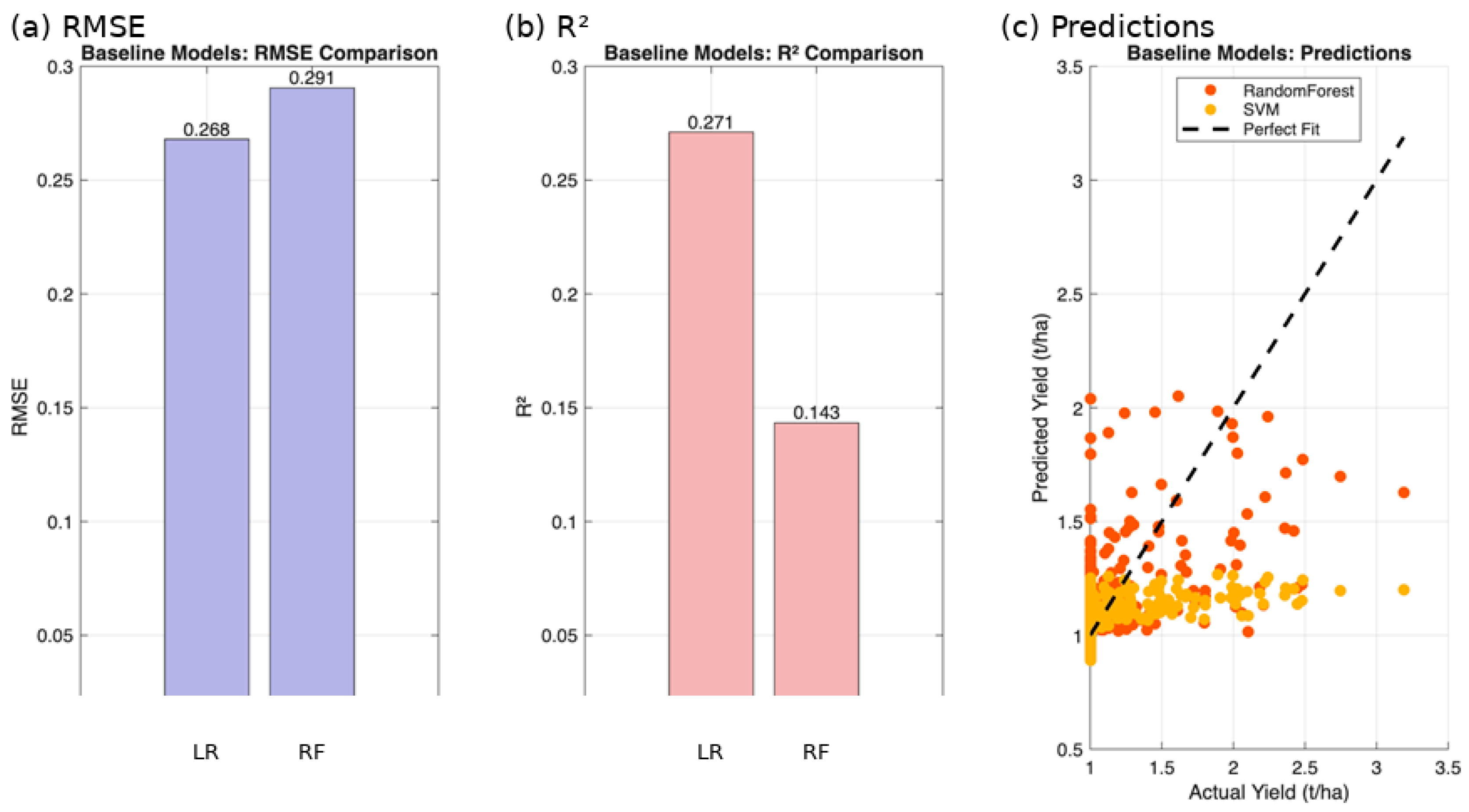
Figure 2 compares the performance of LR and RF on the test set using RMSE, MAE, and R2. RF achieved a lower prediction error (RMSE = 0.268 t/ha) than LR (RMSE = 0.291 t/ha). This corresponds to 18–22% of the mean observed yield (1.2–1.5 t/ha). This level of error is considered moderate for rainfed yield forecasting and reflects the intrinsic uncertainty of climate-driven production systems.
As Figure 2 shows, RF outperforms LR in predictive accuracy and explained variance. Specifically, RF attains a lower RMSE and a higher R2 (0.271) than LR (0.143), indicating superior generalization performance on the temporally held-out test set. Although these R2 values may appear modest, they are consistent with prior studies employing strict chronological validation in rainfed systems where unobserved management practices, socioeconomic heterogeneity, and extreme climatic events constrain the achievable explanatory power.
Predicted versus observed yield plots further highlight structural differences between the models. RF closely tracks observed yields at low-to-moderate production levels (0–1.5 t/ha), but it underestimates higher yields (≥2.5 t/ha). This behavior reflects RF’s capacity to capture nonlinear climate–yield responses under moisture-limited conditions while avoiding overconfident extrapolation beyond the dominant yield range. Overall, the consistent improvement in error- and variance-based metrics confirms the suitability of ensemble learning for yield prediction under heterogeneous, temporally evolving rainfed conditions.
It is important to note that the RF performance reported here (RMSE = 0.268 t/ha; R2 = 0.271) was computed using the temporally held-out test set and the evaluation protocol that were applied throughout the study. These values therefore constitute the reference RF performance under strict chronological validation and are directly comparable with subsequent benchmarking analyses. Any apparent differences observed in later figures arise from changes in the comparison model or diagnostic perspective rather than variations in RF predictive performance.

3.3. Visualizations of Yield and Climatic Relationships

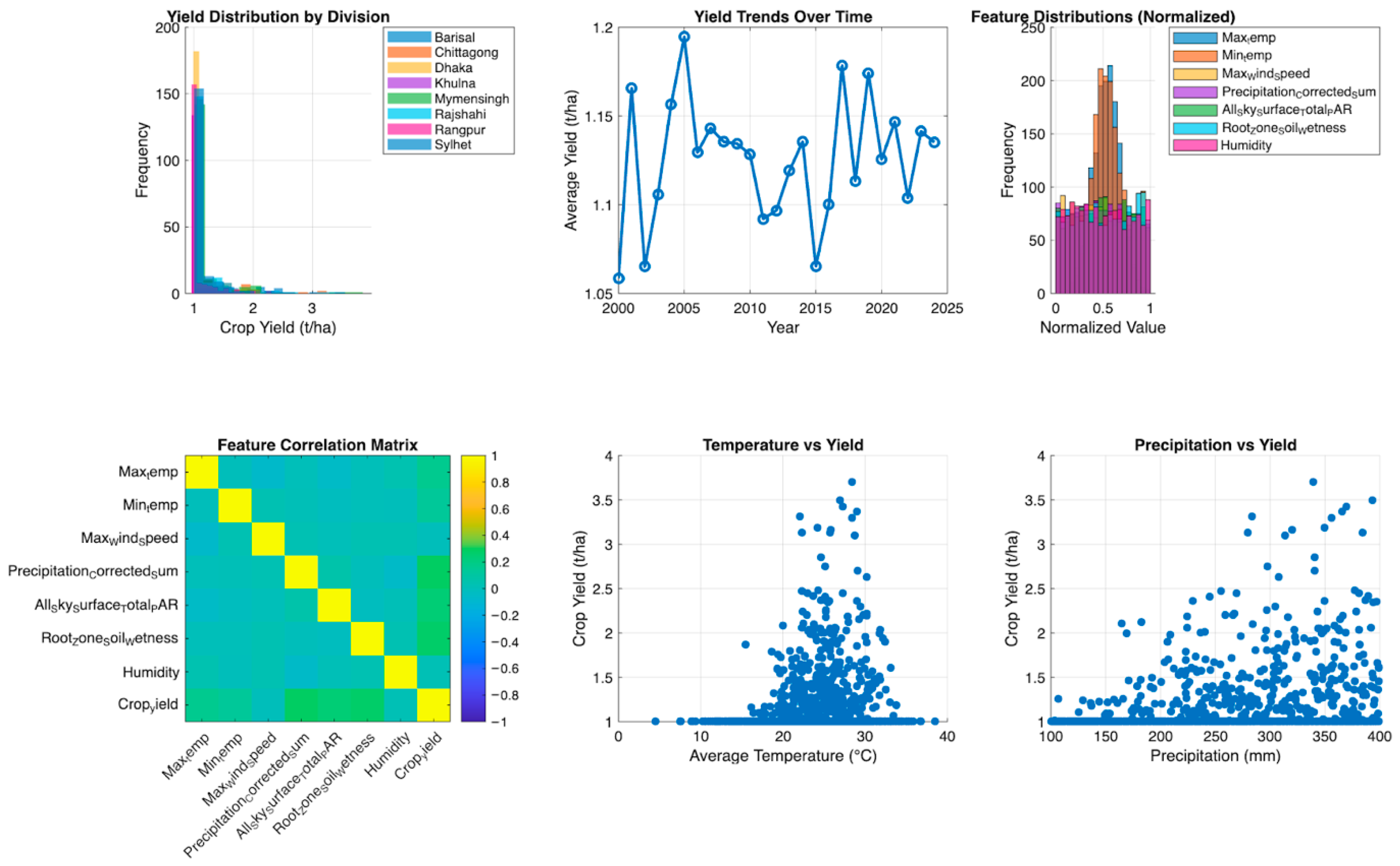
Figure 3 summarizes the spatial, temporal, and agroclimatic structure of the dataset. Yield distributions exhibit pronounced regional heterogeneity and right skewness. Most observations are concentrated between 1.0 and 1.5 t/ha, and there are few high-yield cases exceeding 3.0 t/ha. Regions such as Bihar and Uttar Pradesh demonstrate a high incidence of low-yield outcomes (<1.0 t/ha), which is consistent with their significant exposure to rainfall variability in rainfed systems.
Temporal analysis over the 2000–2025 period reveals moderate interannual fluctuations in average yields, with no strong monotonic trend. This reflects the dominant influence of climatic variability rather than sustained productivity gains.
Normalized feature distributions generally exhibit unimodal but heterogeneous patterns across agroclimatic variables. Temperature-related predictors display relatively narrow and concentrated distributions, whereas precipitation exhibits wider dispersion and heavier tails, highlighting its episodic and highly variable nature. Correlation analysis confirms strong collinearity among temperature variables (ρ ≈ 0.8) and moderate associations between precipitation and relative humidity (ρ ≈ 0.6).
Scatter plots further illustrate nonlinear yield responses to both temperature and precipitation. Yields increase at moderate temperature ranges (10–20 °C), but diminish beyond 30 °C, consistent with the effects of heat stress. Yield–precipitation relationships exhibit weak positive associations accompanied by high dispersion, particularly under extreme rainfall conditions (>300 mm). These distributional and associational patterns collectively confirm the presence of nonlinear effects, scale heterogeneity, and interaction structures. This motivates the use of ensemble- and kernel-based learning methods in subsequent modeling stages.

3.4. Temporal and Regional Stratification of the Dataset

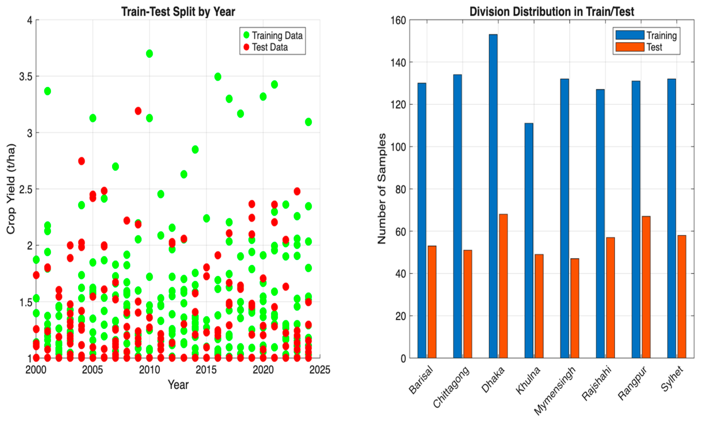
Figure 4 illustrates the temporal and regional evaluation framework adopted in this study. A strict forward-chaining strategy was applied, with observations from 2000 to 2015 assigned to the training set and observations from 2016 to 2025 to the independent test set. This design prevents temporal information leakage and reflects realistic forecasting conditions.
Proportional representation was maintained across the eight administrative divisions: Barisal, Chittagong, Dhaka, Khulna, Mymensingh, Rajshahi, Rangpur, and Sylhet. Each division contributed approximately 110–155 observations to the training period and 45–70 observations to the test period. This corresponds to roughly 20–40% of the samples that were held out for evaluation.
This stratified temporal-regional design enables a robust assessment of model generalization across time and space, aligning the empirical evaluation with the operational objectives of climate-driven yield forecasting.

3.5. Benchmarking: Random Forest vs. Support Vector Regression

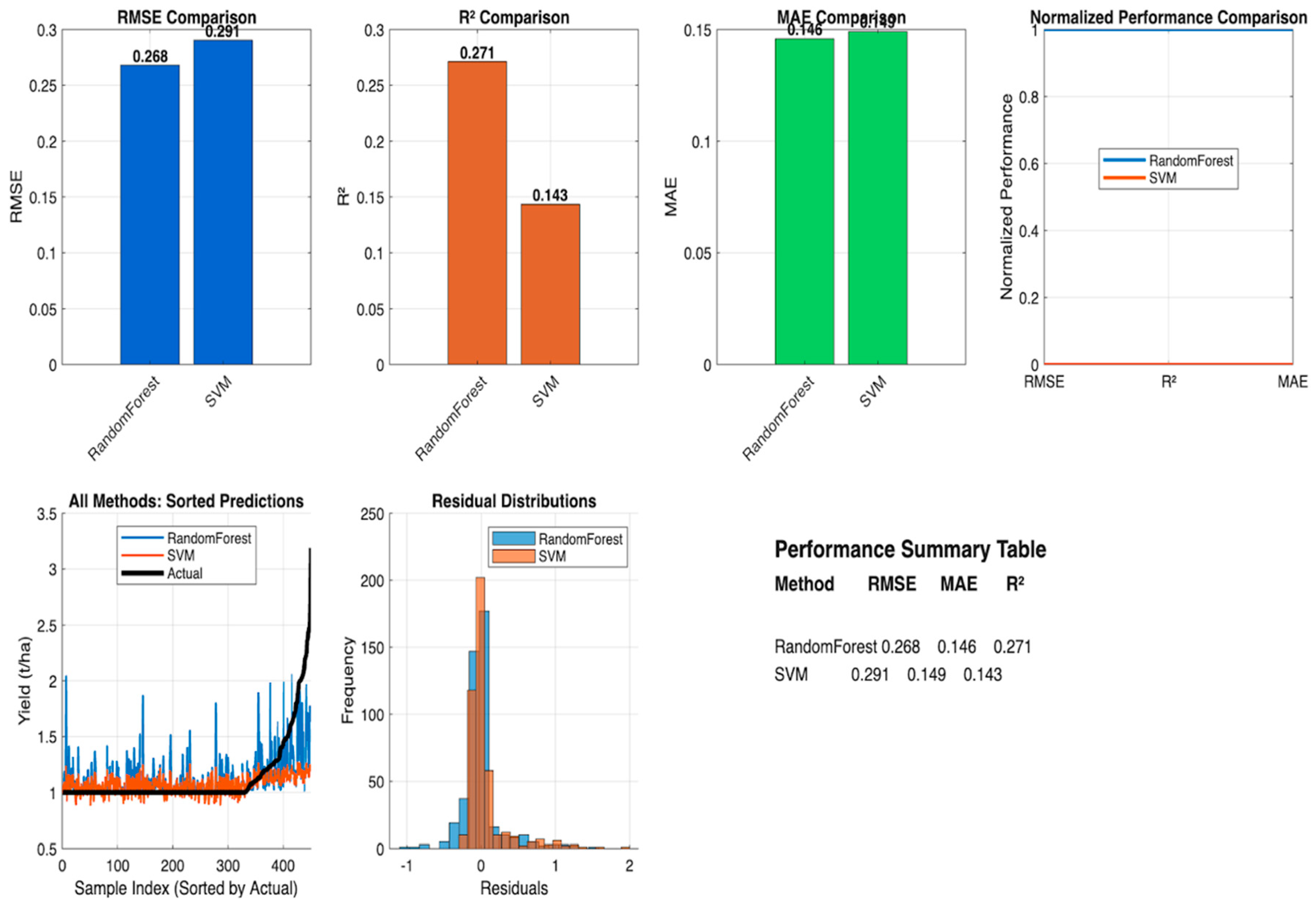
RF performance metrics reported in this section are the same as those in Section 3.2 and Figure 2. Specifically, RF achieves an RMSE of 0.268 t/ha and an R2 of 0.271 using the same chronologically held-out test set. Figure 5 does not present a new evaluation of RF. Rather, it contrasts RF with SVR using the same preprocessing, validation, and metric definitions. Therefore, any apparent differences between Figure 2 and Figure 5 are due to the different comparison model and visualization focus, not changes in RF predictive performance.
Figure 5 provides a detailed comparative assessment of RF and SVR on the independent test set. RF outperforms SVR consistently across all evaluation metrics, achieving a lower RMSE (0.268 t/ha vs. 0.291 t/ha) and higher explained variance (R2 = 0.271 vs. 0.143). While the difference in mean absolute error (MAE) is modest (RF: 0.146 t/ha; SVR: 0.149 t/ha), the normalized performance profiles and sorted prediction plots demonstrate that RF more closely aligns with the observed yields, especially at higher production levels (>2.5 t/ha).
Residual diagnostics further emphasize the structural differences between the models. RF residuals are comparatively narrow and symmetric (approximately −1 to 1 t/ha), whereas SVR residuals exhibit wider dispersion and slight positive skewness. This indicates reduced robustness under extreme yield conditions. Taken together, these results confirm the superior stability and generalization capacity of RF under strict temporal validation (Table 1).

3.6. Performance Evaluation of the Proposed LFSVR Hybrid Model

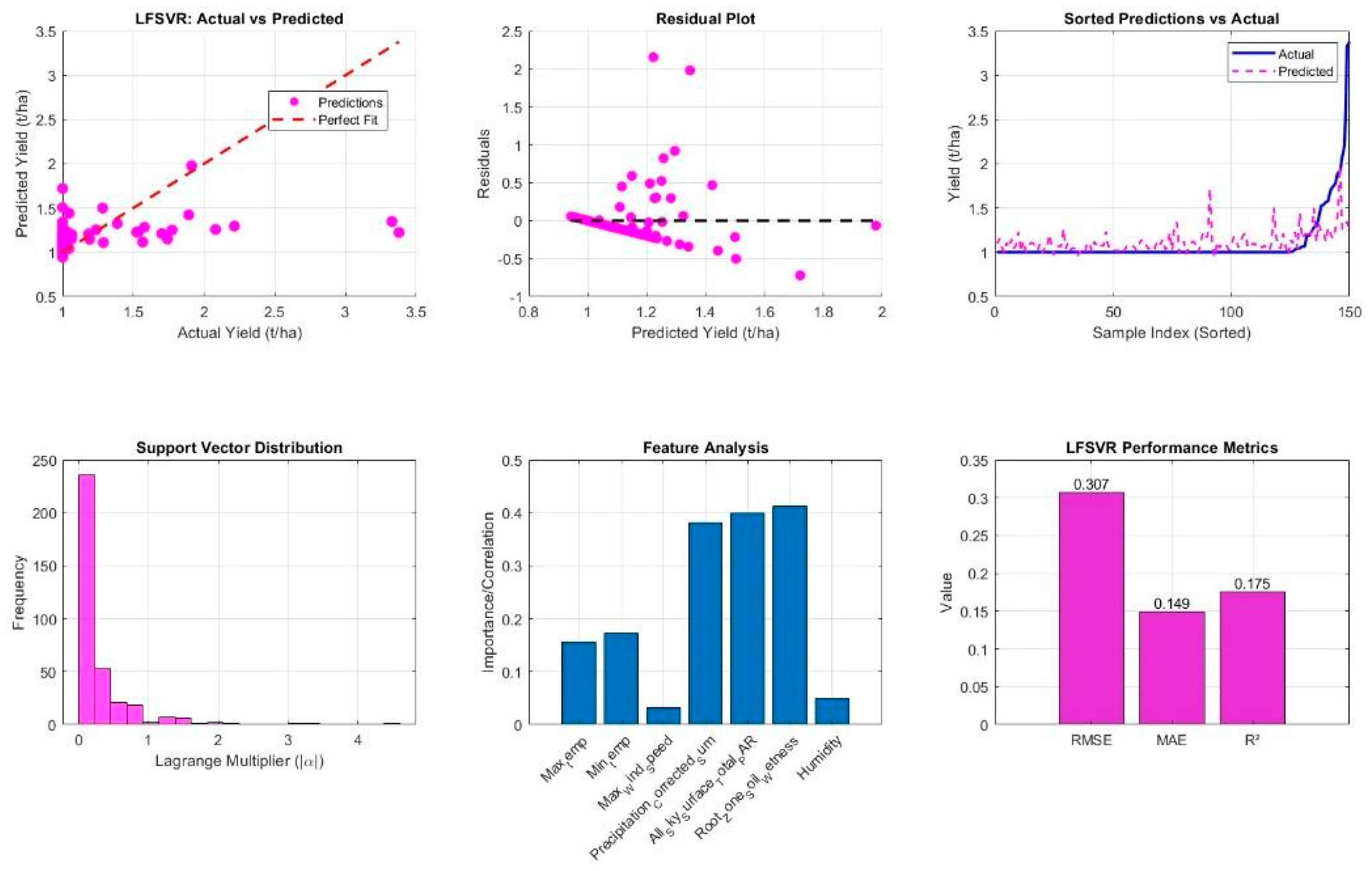
Figure 6 presents a comprehensive diagnostic assessment of the predictive behavior of the Linear–Forest–Support Vector Regression (LFSVR) hybrid model, as evaluated on an independent test set. The actual versus predicted yield plot shows that most predictions are concentrated within a narrow range of approximately 1.0 to 1.5 tons per hectare (t/ha) and increasingly deviate from the 1:1 reference line at higher observed yields. This indicates a systematic underestimation of extreme values. This behavior is confirmed by the plot of sorted predictions versus actual yields, in which predicted values exhibit limited dispersion while observed yields increase sharply in the upper tail. This reveals reduced sensitivity to high-yield observations.
Residual diagnostics indicate a non-random structure with increasing variance at higher yield levels. This suggests the presence of bias and potential heteroscedasticity rather than purely random errors. The distribution of support vectors shows that many observations contribute to the SVR component, which is typical of kernel-based models, but it may also reflect limited generalization capacity under noisy and heterogeneous conditions. Feature contribution analysis highlights soil moisture-related variables, accumulated precipitation, and temperature indicators as dominant predictors, which is consistent with rainfed production systems from an agronomic perspective.
Despite this physically plausible feature structure, the LFSVR model’s overall test-set performance remains limited (RMSE ≈ 0.31 t/ha, MAE ≈ 0.15 t/ha, and R2 ≈ 0.18). These results indicate weak explanatory power and confirm that the hybrid model does not outperform the Random Forest baseline under strict chronological validation.
Consistent with the methodological framework described in Section 2, the LFSVR model was evaluated using the same dataset, preprocessing workflow, and forward-chaining train–test split as the baseline models. The hybrid architecture was implemented as a stacked learning framework in which linear regression, random forest, and support vector regression served as base learners and a linear meta-learner integrated their out-of-fold predictions. The base models were trained using five-fold cross-validation on the 2000–2015 period, and the final performance was assessed on the independent test period from 2016 to 2025 using RMSE, MAE, and R2.
Overall, the LFSVR framework integrates complementary modeling paradigms: linear trends, nonlinear interactions, and kernel-based generalization. However, the additional complexity does not translate into improved predictive accuracy or robustness under realistic forecasting conditions. These findings suggest that given the present data regime and the high signal-to-noise ratio characteristic of rainfed agricultural systems, hybrid stacking does not necessarily yield performance gains over a well-calibrated ensemble baseline, such as RF.

4. Discussion

Section 3 provides quantitative evidence of the performance of different machine learning paradigms under strict chronological validation in rainfed agricultural systems. At first glance, the coefficient of determination obtained for the Random Forest (RF) model (R2 = 0.271) may seem modest compared to values reported in studies based on random or spatially mixed data partitions. However, this level of explained variance must be interpreted in the context of forward-chaining validation, multi-division heterogeneity, and the exclusive use of agroclimatic predictors. In rainfed systems, yield variability is strongly influenced by unobserved management practices, socioeconomic conditions, and extreme climatic events. These factors inherently constrain achievable R2 values under realistic forecasting settings. As in prior research, chronological validation yields more conservative yet operationally reliable performance estimates, while random splits tend to inflate accuracy metrics. Thus, this study’s contribution lies not in maximizing R2, but in establishing a reproducible, decision-relevant benchmark aligned with real-world forecasting conditions.
Beyond statistical accuracy, these results have direct implications for the practical use of yield forecasts in climate-sensitive decision-making. This section interprets the empirical findings in relation to existing literature and discusses their relevance to operational forecasting, resource management, and risk-informed planning in rainfed agriculture. A consistency check of the reported metrics confirms that Random Forest performance is identical across all comparative figures because it is computed using the same chronologically held-out test set. Thus, RF performance remains consistently at RMSE = 0.268 t/ha and R2 = 0.271. An earlier labeling inconsistency in Figure 2 has been corrected to ensure full alignment with the validated results presented in Figure 5.

4.1. Interpretation of LFSVR Hybrid Model Performance

The empirical results indicate that the Linear–Forest–Support Vector Regression (LFSVR) framework does not outperform the Random Forest baseline under strict chronological validation. This can be understood by considering the interaction between the model’s structure, the data’s characteristics, and the validation design.
Random Forest already captures a significant portion of the nonlinear signal embedded in the agroclimatic predictors through ensemble-based partitioning. Under these conditions, additional learners operating within the same input space provide minimal independent information. Consequently, the stacking strategy aggregates correlated prediction structures rather than exploiting complementary error patterns, yielding marginal or negative gains in generalization.
Furthermore, the stacked architecture inherits uncertainty from its constituent models. When base learners exhibit heterogeneous but systematically weaker performance than the ensemble reference, the meta-learning stage may amplify bias rather than mitigate it. Using a linear meta-learner further constrains the variability of combined predictions, reducing sensitivity to extreme yield realizations and limiting explanatory capacity under temporally evolving conditions.
The strict forward-chaining validation strategy accentuates these effects further. Hybrid and stacked models benefit from random or spatially mixed validation schemes that allow partial information overlap across folds. In contrast, chronological validation mirrors operational forecasting constraints and penalizes model complexity, favoring parsimonious architectures with stable inductive biases.
Finally, this study intentionally restricts the predictive space to agroclimatic and soil variables. Without management, socioeconomic, or remotely sensed inputs, increasing architectural complexity does not compensate for limited explanatory content. Under such data regimes, a well-calibrated ensemble model can achieve greater robustness than more elaborate hybrid designs.

4.2. Managerial Implementation and Strategic Implications for Precision Agribusiness

Machine learning (ML) models, particularly Random Forest (RF) and Support Vector Regression (SVR), offer substantial potential for improving decision-making in precision agriculture [34]. This study’s empirical results demonstrate that RF outperforms SVR under rainfed conditions (root mean square error [RMSE]: 0.268 vs. 0.291 tons per hectare [t/ha]; R2: 0.271 vs. 0.143), particularly in capturing nonlinear climate–yield relationships. These results highlight the importance of ML-based tools for agribusiness firms, government agencies, and farmer cooperatives that want to develop more climate-resilient planning strategies.
Effective implementation requires a phased managerial approach aligned with best practices in digital agriculture. Initial efforts should focus on auditing and harmonizing existing yield and climate datasets (e.g., ICAR and IMD records) using standardized preprocessing and temporal validation protocols. Prioritizing open-source ML ecosystems can help maintain implementation costs within 5–10% of annual operational budgets [35]. Subsequent model adaptation to regional agroclimatic conditions can leverage RF feature-importance diagnostics to identify precipitation as a key yield driver in drought-prone regions and apply strict chronological validation to prevent temporal leakage. Pilot deployments in data-rich divisions may achieve forecast accuracies within ±15%, supporting improved irrigation planning, input procurement, and inventory management.
At scale, ML models can be embedded within cloud-based decision support systems and augmented with real-time IoT observations to enhance operational responsiveness. For example, RF-driven dashboards could allow cooperatives to detect yield anomalies associated with extreme temperature events (above 30 °C) relative to historical baselines. This would support timely, data-informed management interventions in rainfed systems [36].

4.3. Operational Benefits for Agribusiness

The managerial value of machine learning (ML)-based forecasting lies in its ability to translate predictive insights into operational efficiencies. The symmetric residual structure observed in the RF model reduces the risk of systematic over- or underestimation (Figure 5). This enables more targeted fertilizer application and the potential reduction of input use by 10–20%. This reduction is consistent with the sustainability objectives of SDG 2.
Improved forecast accuracy contributes to greater supply chain stability. It does so by mitigating procurement volatility in markets where annual price fluctuations can approach 30% (FAO, 2024). Additionally, scenario-based simulations under rainfall deficits demonstrate how SVR’s resilience to outliers can complement RF’s accuracy in probabilistic forecasting, supporting climate risk management with yield forecasts approaching 70% confidence levels. Integrating these forecasts into digital advisory platforms like the Kisan Suvidha portal could provide over 150 million farmers with timely guidance. Evidence from comparable contexts, including ML-driven soybean forecasting in Brazil, suggests that data-driven yield prediction can improve productivity by up to 15%. This underscores the broader applicability of ML-based forecasting across rainfed systems [37].
From a practical perspective, the proposed modeling framework can support climate-sensitive decision-making in rainfed agricultural systems. For example, probabilistic yield forecasts generated before the planting or early growing season can inform fertilizer application timing by discouraging early input intensification in years with elevated drought risk, thereby reducing unnecessary costs and environmental losses. Similarly, yield forecasts with quantified error ranges can support index-based crop insurance schemes by providing objective, climate-driven benchmarks for indemnity triggers.

4.4. Challenges and Constraints for Real-World Implementation

Despite the benefits of ML-based forecasting systems, several challenges constrain their deployment. Data scarcity and imbalance are critical issues that affect model reliability, as illustrated by skewed yield distributions and limited sample density in regions such as Jharkhand (Figure 3). Data-sharing initiatives and appropriate resampling strategies may mitigate these limitations. The “black box” nature of RF models poses a barrier to stakeholder trust, but post hoc explainability methods such as SHAP can address this concern by identifying the contributions of key predictors, including precipitation and temperature. Scalability and equity issues persist as well, as the high computational demands of these models may hinder their adoption by smallholder cooperatives. Low-cost edge computing solutions and tiered access to decision support systems can enhance inclusivity (e.g., Raspberry Pi clusters < $500) and tiered DSS access can enhance inclusivity. Ethical considerations are also relevant because ML models may inadvertently favor high-yield regions due to sample imbalance. This underscores the need for regular fairness audits.

4.5. Synthesis and Broader Implications

In summary, implementing RF and SVM models for crop yield prediction provides agribusiness leaders with a robust, scalable toolkit for navigating climatic uncertainty. Phased adoption yields measurable gains in efficiency, resilience, and sustainability [38].
Combining predictive analytics with strategic planning has the potential to elevate India’s agricultural sector to a projected valuation of USD 500 billion by 2030. Managers are encouraged to initiate pilot implementations in 2026 and engage in academic–industry collaborations to make iterative improvements.

4.6. Limitations of the Research

This study identifies five major gaps in the existing literature and acknowledges that the present analysis does not fully resolve all of these challenges. The proposed framework addresses the need for a unified benchmarking strategy with strict temporal validation and improves robustness with ensemble and hybrid learning. However, limitations remain regarding the explicit modeling of extreme climate events, integrating socioeconomic and management variables, quantifying uncertainty comprehensively, and deploying the framework on a large scale.
These gaps largely reflect constraints in data availability and the study’s deliberate focus on establishing a reliable, climate-driven baseline rather than a fully integrated decision-support system. Accordingly, the gaps should be viewed as a structured research agenda rather than as deficiencies of the proposed approach, inspiring future extensions such as probabilistic forecasting, the incorporation of management practices, and real-time deployment frameworks.
Several limitations should be considered when interpreting the empirical results. First, the dataset is imbalanced and skewed regionally, particularly in states such as Jharkhand and Chhattisgarh, where yield distributions are concentrated in lower ranges (Figure 3). This uneven representation may constrain model generalization in underrepresented regions [39].
Second, the analysis relies exclusively on agroclimatic and soil variables. This excludes potentially influential socioeconomic and management factors, such as fertilizer application rates, cultivar selection, and irrigation practices. This may limit the models’ ability to fully explain yield variability in heterogeneous farming systems. Illumination-related variables, such as sunshine duration and solar radiation, influence crop growth through photosynthesis; however, they were not included in the present analysis. This is due to the lack of long-term, spatially consistent illumination datasets covering all administrative divisions and the full study period. To maintain temporal continuity, regional comparability, and balanced sample coverage while ensuring strict chronological validation, the model was restricted to agroclimatic variables that were consistently available across regions and years. Consequently, the results should be interpreted as a climate-driven baseline rather than a comprehensive representation of all biophysical yield determinants.
Third, while strict chronological train-test splits effectively reduce temporal leakage, the analysis does not capture climate dynamics beyond the 2000–2025 period. This restricts long-term extrapolation under future climate regimes. Incorporating downscaled climate projections or CMIP6 scenarios would improve forward-looking assessments.
Model interpretability remains a challenge as well. While Random Forest and Support Vector Regression demonstrate strong predictive performance, their internal complexity limits transparency. Although SHAP-based post hoc explanations partially address this issue, interpretability constraints may hinder adoption by nontechnical stakeholders.
Finally, computational requirements may limit scalability among smallholder cooperatives. Although low-cost edge computing solutions are feasible, full operational deployment depends on stable digital infrastructure, which is uneven across regions of India.
Regarding generalizability, the models were trained and evaluated using multi-year data spanning diverse climatic conditions, which supports their applicability across seasons within the same crop system. The present analysis focuses on a single crop and a defined set of administrative divisions; however, the framework is crop-agnostic and can be extended to other rainfed crops with comparable agroclimatic and yield data. However, cross-crop transferability and performance under substantially different phenological cycles require further empirical validation.
Future research should build on the benchmarking framework introduced in this study. Priority areas for future research include integrating satellite-derived vegetation indices, assessing model transferability across crops and agroecological contexts under consistent preprocessing and validation protocols, and incorporating uncertainty quantification and rolling-window validation. These extensions are intended to refine, rather than fundamentally alter, the proposed framework, thereby enhancing its operational relevance for risk-sensitive agricultural decision-making.

5. Conclusions

This study provides a comprehensive, methodologically rigorous benchmarking assessment of three widely used machine learning models—linear regression, random forest (RF), and support vector regression (SVR)—for predicting yields in rainfed cereal systems across eight Indian administrative divisions from 2000 to 2025. Through the use of standardized preprocessing, strict chronological train–test partitioning, and extensive exploratory data analysis, the study shows that RF provides the most reliable predictive performance under realistic forecasting conditions. RF achieves the lowest test error (RMSE = 0.268 t/ha; MAE = 0.146 t/ha) and the highest explained variance (R2 = 0.271). RF outperforms SVR (RMSE = 0.291 t/ha, R2 = 0.143) and linear regression, confirming the advantages of ensemble-based learning for modeling nonlinear climate–yield relationships in rainfed environments.
These results underscore the importance of adopting machine learning frameworks evaluated under realistic temporal validation, especially in systems with strong climatic variability, moderate temporal persistence (φ ≈ 0.65), and heterogeneous agroclimatic dependencies. Examples include the weak yet significant association between precipitation and yield (ρ ≈ 0.1). Importantly, the reported performance levels reflect conservative and operationally relevant forecasting skill because strict chronological validation avoids the optimistic bias commonly associated with random or spatially mixed data partitions.
The proposed linear–forest–support vector regression (LFSVR) hybrid model did not outperform the random forest baseline under the present data regime. Although the goal of hybridization was to combine complementary inductive biases, the additional modeling complexity did not result in better generalization when evaluated on an independent, chronologically held-out test set. This finding underscores that in climate-noisy rainfed systems with limited covariate coverage, more complex hybrid architectures do not necessarily outperform well-calibrated ensemble baselines.
From an applied perspective, the study provides a robust methodological foundation for operational, machine learning-based yield forecasting in agribusiness and public-sector decision-making. The division-stratified and temporally consistent evaluation design enhances generalizability and supports actionable insights for resource allocation, supply chain stabilization, and climate-smart agricultural management, which aligns with SDG 2 (Zero Hunger) [40]. Given the IPCC’s (2022) projections of potential yield declines of 5–15% by 2030 due to increasing monsoon irregularity, the demonstrated robustness of RF offers a scalable, cost-effective decision support tool. Its symmetric residual structure and interpretable feature-importance profiles support more efficient fertilizer use, potentially reducing inputs by 10–20%, and contribute to improving the resilience of India’s predominantly smallholder-based rainfed agricultural systems.

Future Research

Future research should build incrementally on the benchmarking framework established in this study rather than pursuing multiple parallel extensions. A priority direction is the integration of additional data sources, including satellite-derived vegetation indices and spatiotemporal information, to assess whether they improve predictive accuracy under the same strict chronological validation strategy. Further work should evaluate the transferability of both baseline and hybrid models across different rainfed crops and agroecological contexts while maintaining consistent preprocessing and evaluation protocols. Incorporating uncertainty quantification, rolling-window validation, and climate scenario analysis would further enhance the operational relevance of forecasts for risk-sensitive applications such as input management and index-based insurance. These extensions are intended to refine, rather than fundamentally alter, the standardized and operationally realistic benchmarking approach introduced in this study.

Author Contributions

Conceptualization, A.K.Y.; Methodology, A.K.Y.; Software, A.K.Y.; Validation, C.D.; Formal analysis, C.D.; Investigation, C.D.; Resources, I.D.; Data curation, I.D.; Writing—original draft, I.D. and G.V.G.; Writing—review & editing, G.V.G.; Supervision, A.K.Y. and G.V.G.; Project administration, A.K.Y.; Funding acquisition, G.V.G. All authors have read and agreed to the published version of the manuscript.

Funding

Amir Karbassi Yazdi and Gonzalo Valdez thank the financial support from Fortalecimiento Grupos de Investigación UTA N° 8764-25.

Data Availability Statement

The original contributions presented in this study are included in the article. Further inquiries can be directed to the corresponding author.

Acknowledgments

Gonzalo Valdes would like to acknowledge the help and support from UTA Mayor 8763-25.

Conflicts of Interest

The authors declare no conflicts of interest.

Abbreviations

The following abbreviations are used in this manuscript:
RFRandom Forest
SVMSupport Vector Machine
SVRSupport Vector Regression
LRLinear Regression
LSTMLong Short-Term Memory Network
NDVINormalized Difference Vegetation Index
EVIEnhanced Vegetation Index
MODISModerate Resolution Imaging Spectroradiometer
AR(1)First-Order Autoregressive Model
JBJarque–Bera Statistic
DWDurbin–Watson Statistic
VIFVariance Inflation Factor
OOBOut-of-Bag Error
CVCross-Validation
AICAkaike Information Criterion
IQRInterquartile Range
RMSERoot Mean Square Error
MAEMean Absolute Error
R2Coefficient of Determination
IoTInternet of Things
SDGSustainable Development Goals
RSSResidual Sum of Squares
BPBreusch–Pagan Test
QLjung–Box Statistic

Appendix A

Table A1. Symbols, definitions, and context used in the study.
Symbol/VariableDefinitionContext
n Total number of observations/samples in the dataset (e.g., n ≈ 1250)Preprocessing
y Target variable: Crop yield (tons per hectare, t/ha), with range y ∈ [0.5,4] Dataset description
X X = x 1 , , x 7 ,   where   each   x i is a normalized environmental featureModel formulation Predictor matrix
x i Individual predictor variable i   ( for   i = 1 , , 7 ): e.g., MaxTemp (maximum temperature, °C), MinTemp (minimum temperature, °C), AvgTemp (average temperature, °C), Precip (precipitation, mm), RelHum (relative humidity, %), WindSpd (wind speed, m/s), SoilpH (soil pH)Preprocessing
x i Normalized   predictor :   x i = x i μ i σ i Preprocessing
μ i Mean   of   feature   i :   μ i = 1 n j = 1 n x j , i Normalization
σ i Standard deviation of feature i :   σ i = 1 n 1 j = 1 n ( x j , i μ i ) 2 Normalization
D t r a i n Training dataset (80% of data, years 2000–2015, $$)Preprocessing
D t e s t Test dataset (20% of data, years 2016–2025, $$)Preprocessing
γ 1 γ 1 = E [ y y ˉ ) 3 σ y 3   ( E is   expectation ,   y ˉ   is   sample   mean ,   σ y is standard deviation of y )EDA: Skewness coefficient
γ 2 γ 2 = E [ y y ˉ ) 4 σ y 4 3 EDA: Kurtosis
J B J B = n 6 γ 1 2 + γ 2 2 4 χ 2 (chi-squared distribution)EDA: Jarque–Bera
ϕ y t = ϕ y t 1 + ϵ t   ( t   indexes   time ,   ϵ t is white noise)EDA AR(1) model:
D W D W = 2 1 ϕ EDA: Durbin-Watson
R R [ 1 , 1 ] 8 × 8 (8 × 8 including y )EDA: Pearson matrix
r j k   or   ρ j k r j k = c o v x j , x k σ x j σ x k   ( c o v A , B = E A E A B E B )EDA: Pearson correlation coefficient:
I X ; Y I X ; Y = x , y p x , y l o g p x , y p x p y   ( nats ;   p is probability mass function)EDA: Mutual information
V I F V I F j = 1 1 r j 2   ( where   r j 2   is   R 2   from   regressing   x j )EDA: Variance Inflation Factor
y ^   or   y ^ i Predicted yield for observation i Model predictions
β β = [ β 0 , β 1 , , β 7 ] ( β 0 : intercept)LR formulation
x i x i = [ 1 , x i 1 , , x i 7 ] (design matrix row)LR formulation
p Number   of   predictors   ( p = 7 )Model degrees of freedom
R S S Residual   Sum   of   Squares :   R S S = i = 1 n ( y i x i β ) 2 LR estimation
σ ^ 2 Estimated   error   variance :   σ ^ 2 = R S S n p 1 LR inference
B P Breusch-Pagan test statistic: B P = n R a u x 2 χ p 2   ( R a u x 2 :   R 2 from auxiliary regression of squared residuals X )LR: Heteroscedasticity test
B Number   of   trees   in   RF   ensemble   ( B = 100 )RF formulation
T b x Prediction from the b -th decision treeRF aggregation
m Node index in decision treeRF splitting
M S E m Mean Squared Error at node m :   M S E m = k = 1 K w k ( μ k y ˉ m ) 2 RF split criterion
K Number of child nodes at splitRF splitting
w k Weight of child node k :   w k = N k / N m   ( N k :   samples   in   node   k ;   N m :   samples   in   parent   m )RF splitting
μ k Mean   yield   in   child   node   k RF splitting
y ˉ m Mean   yield   in   parent   node   m :   y ˉ m = k = 1 K w k μ k RF splitting
y ^ O O B , i Out-of-bag prediction for observation iRF generalization estimate
I f Feature   importance   for   feature   f :   I f = t T f Δ G i n i t / B   ( T f :   splits   using   f )RF interpretability
Δ G i n i t Δ G i n i t = p l , t 1 p l , t + p r , t 1 p r , t   ( p l , r : proportions in left/right child)RF feature importance
w Weight vector in SVR hyperplaneSVR primal
b Bias term in SVR hyperplaneSVR primal
ξ , ξ * Slack   variables   for   upper / lower   tube   violations   ( ξ i 0 penalizes underestimation)SVR constraints
C Regularization   parameter   in   SVR   ( C = 1 )SVR trade-off
ϵ Tube   width   in   SVR   ( ϵ = 0.1 )SVR insensitivity margin
ϕ x i Feature map to high-dimensional spaceSVR kernel trick
K x i , x j RBF   kernel :   K x i , x j = e x p γ x i x j 2 SVR duality
γ Kernel   bandwidth :   γ = 1 / 2 d σ 2   ( d = 7 : feature dimensionality)SVR RBF
α , α * Lagrange   multipliers   in   SVR   dual   ( 0 α i , α i * C )SVR prediction
S V Set of support vectors (indices where $$ 0 <)\alpha_i − \alpha_i^*
K (CV) Number of folds in cross-validation (K = 5) Training
V k Validation   fold   k in CVCV procedure
y ^ k x i Prediction   for   i   trained   excluding   fold   k CV-MSE
n k Size   of   fold   k CV-MSE
C V M S E Cross-validated Mean Squared Error: C V M S E = 1 K k = 1 K 1 n k i V k ( y i y ^ k x i ) 2 Hyperparameter tuning
A I C Akaike   Information   Criterion :   A I C = n l o g σ ^ 2 + 2 p + 1 Model selection
R M S E Root   Mean   Square   Error :   R M S E = 1 n i = 1 n ( y i y ^ i ) 2 Evaluation
M A E Mean Absolute Error: $$ \text{MAE} = \frac{1}{n} \sum_{i = 1}^ny_i − \hat{y}_i
R 2 Coefficient   of   determination :   R 2 = 1 ( y i y ^ i ) 2 ( y i y ˉ ) 2 Evaluation
R 2 Adjusted   R 2 :   R 2 = 1 1 R 2 n 1 n p 1 Evaluation
Q Ljung–Box statistic: Ljung Box   statistic :   Q = n n + 2 h = 1 H ρ ^ h 2 n h χ H p 2   ( ρ ^ h :   lag - h   autocorrelation ;   H : lags)Residual diagnostics
e j , i Error   for   model   j at   observation   i :   e j , i = y i y ^ j , i Clark-West test
C W Clark-West test statistic: C W = 1 n ( e 1 , i 2 e 2 , i 2 + y ^ 2 , i y ^ 1 , i ) 2 N 0 , σ 2   (for nested models 1 superior to 2)Model comparison

References

  1. Mishra, A.K.; Singh, R. Climate vulnerability in rainfed farming: Analysis from Indian watersheds. Sustainability 2018, 10, 3357. [Google Scholar] [CrossRef]
  2. De Clercq, D.; Mahdi, A. Feasibility of machine learning-based rice yield prediction in India at the district level using climate reanalysis data. arXiv 2024, arXiv:2403.07967. [Google Scholar] [CrossRef]
  3. Xu, T.; Guan, K.; Peng, B.; Wei, S.; Zhao, L. Machine learning-based modeling of spatio-temporally varying responses of rainfed corn yield to climate, soil, and management in the U.S. Corn Belt. Front. Artif. Intell. 2021, 4, 647999. [Google Scholar] [CrossRef] [PubMed]
  4. Paudel, D.; de Wit, A.; Boogaard, H.; Marcos, D.; Osinga, S.; Athanasiadis, I.N. Interpretability of deep learning models for crop yield forecasting. Comput. Electron. Agric. 2023, 206, 107663. [Google Scholar] [CrossRef]
  5. Khaki, S.; Wang, L. Crop yield prediction using deep neural networks. Front. Plant Sci. 2019, 10, 621. [Google Scholar] [CrossRef]
  6. Chlingaryan, A.; Sukkarieh, S.; Whelan, B. Machine learning approaches for crop yield prediction and nitrogen status estimation in precision agriculture: A review. Comput. Electron. Agric. 2018, 151, 61–69. [Google Scholar] [CrossRef]
  7. Kuradusenge, M.; Hitimana, E.; Hanyurwimfura, D.; Rukundo, P.; Mtonga, K.; Mukasine, A.; Uwitonze, C.; Ngabonziza, J.; Uwamahoro, A. Crop yield prediction using machine learning models: Case of Irish potato and maize. Agriculture 2023, 13, 225. [Google Scholar] [CrossRef]
  8. Hoque, M.J.; Islam, M.S.; Uddin, J.; Samad, M.A.; Sainz-De-Abajo, B.; Ramírez Vargas, D.L.; Ashraf, I. Incorporating meteorological data and pesticide information to forecast crop yields using machine learning. IEEE Access 2024, 12, 47768–47786. [Google Scholar] [CrossRef]
  9. Sintayehu, G.; Ebstu, E.T.; Akili, D. Assessment of surface irrigation potential availability using GIS in Gilgel Abbay Catchment, Ethiopia. Res. Sq. 2022. [Google Scholar] [CrossRef]
  10. Kirthiga, S.M.; Patel, N.R. In-season wheat yield forecasting at high resolution using regional climate model and crop model. AgriEngineering 2022, 4, 1054–1075. [Google Scholar] [CrossRef]
  11. Tesfaye, K.; Takele, R.; Shelia, V.; Lemma, E.; Dabale, A.; Traoré, P.C.S.; Solomon, D.; Hoogenboom, G. High spatial resolution seasonal crop yield forecasting for heterogeneous maize environments in Oromia, Ethiopia. Clim. Serv. 2023, 32, 100425. [Google Scholar] [CrossRef]
  12. Ordoñez, L.; Vallejo, E.; Amariles, D.; Mesa, J.; Esquivel, A.; Llanos-Herrera, L.; Prager, S.D.; Segura, C.; Valencia, J.J.; Duarte, C.J.; et al. Applying agroclimatic seasonal forecasts to improve rainfed maize management in Colombia. Clim. Serv. 2022, 28, 100333. [Google Scholar] [CrossRef]
  13. Miao, L.; Zou, Y.; Cui, X.; Kattel, G.R.; Shang, Y.; Zhu, J. Predicting China’s maize yield using multi-source datasets and machine learning algorithms. Remote Sens. 2024, 16, 2417. [Google Scholar] [CrossRef]
  14. Wanthanaporn, U.; Supit, I.; Chaowiwat, W.; Hutjes, R.W.A. Skill of rice yield forecasting over Mainland Southeast Asia using ECMWF SEAS5 and WOFOST. Agric. For. Meteorol. 2024, 351, 110001. [Google Scholar] [CrossRef]
  15. Ghosh, S.; Mukhoti, S.; Sharma, P. Quantifying rainfall-induced climate risk in rainfed agriculture. Agric. Water Manag. 2025, 319, 109775. [Google Scholar] [CrossRef]
  16. Park, S.; Chun, J.A.; Kim, D.; Sitthikone, M. Climate risk management for rainfed rice yield using APCC MME forecasts. Agric. Water Manag. 2022, 274, 107976. [Google Scholar] [CrossRef]
  17. Jeong, J.H.; Resop, J.P.; Mueller, N.D.; Fleisher, D.H.; Yun, K.; Butler, E.E.; Timlin, D.J.; Shim, K.-M.; Gerber, J.S.; Reddy, V.R.; et al. Random forests for global and regional crop yield predictions. PLoS ONE 2016, 11, e0156571. [Google Scholar] [CrossRef]
  18. Shahhosseini, M.; Hu, G.; Archontoulis, S.V. Forecasting corn yield with machine learning ensembles. Front. Plant Sci. 2021, 12, 709008. [Google Scholar] [CrossRef]
  19. van Klompenburg, T.; Kassahun, A.; Catal, C. Crop yield prediction using machine learning: A systematic literature review. Comput. Electron. Agric. 2020, 177, 105709. [Google Scholar] [CrossRef]
  20. Hyndman, R.J.; Athanasopoulos, G. Forecasting: Principles and Practice, 2nd ed.; OTexts: Melbourne, Australia, 2018; Available online: https://otexts.com/fpp2/ (accessed on 20 August 2025).
  21. Hastie, T.; Tibshirani, R.; Friedman, J. The Elements of Statistical Learning, 2nd ed.; Springer: Berlin/Heidelberg, Germany, 2009. [Google Scholar]
  22. Box, G.E.P.; Jenkins, G.M.; Reinsel, G.C.; Ljung, G.M. Time Series Analysis: Forecasting and Control, 5th ed.; Wiley: Hoboken, NJ, USA, 2015. [Google Scholar]
  23. Sharma, A.; Mehrotra, R. An information-theoretic alternative for hydrologic forecasting evaluation. J. Hydrol. 2014, 512, 90–103. [Google Scholar]
  24. Wooldridge, J.M. Introductory Econometrics: A Modern Approach, 6th ed.; Cengage Learning: Boston, MA, USA, 2016. [Google Scholar]
  25. Kuhn, M.; Silge, J. Tidy Modeling with R, 2nd ed.; O’Reilly Media: Sebastopol, CA, USA, 2024. [Google Scholar]
  26. Vapnik, V. The Nature of Statistical Learning Theory; Springer: Berlin/Heidelberg, Germany, 1995. [Google Scholar]
  27. Wolpert, D.H. Stacked generalization. Neural Netw. 1992, 5, 241–259. [Google Scholar] [CrossRef]
  28. Prasad, R.; Ahmad, A. A hybrid feature selection and ML framework for yield prediction. In Neural Computing and Applications; Springer: Berlin/Heidelberg, Germany, 2024. [Google Scholar] [CrossRef]
  29. Zhang, Y.; Zhao, Y.; Wang, H. A stacking ensemble framework for forest biomass estimation. GISci. Remote Sens. 2025, 62, 230–247. [Google Scholar]
  30. Li, X.; Zhang, Y.; Chen, Q. Comparative evaluation of ML models for maize yield under climate variability. Comput. Electron. Agric. 2023, 209, 107995. [Google Scholar]
  31. Jarro-Espinal, I.; Huanuqueño-Murillo, J.; Quille-Mamani, J.; Quispe-Tito, D.; Ramos-Fernández, L.; Pino-Vargas, E.; Torres-Rua, A. Field-scale rice yield prediction in Peru using LR, RF, and SVR. Agriculture 2025, 15, 2054. [Google Scholar] [CrossRef]
  32. Rathod, S.; Sailaja, B.; Bandumula, N.; Kumar, S.A.; Prasanna, P.A.L.; Jeyakumar, P.; Waris, A.; Muthuraman, P.; Sundaram, R.M. Time Series and Artificial Intelligence Models for Forecasting Agricultural Data; ICAR-IIRR: Haiderabad, India, 2023. [Google Scholar]
  33. García, L.; González-Sánchez, A.; Jiménez, F.; Castellanos, J. Best practices for ML in crop yield prediction. Comput. Electron. Agric. 2023, 210, 107893. [Google Scholar]
  34. Khanna, A.; Kaur, S.; Gupta, R. Cloud-edge AI architectures for precision agriculture. Comput. Electron. Agric. 2024, 215, 108560. [Google Scholar]
  35. Ramaprasad, A.; Gowrish, R.; Mehta, V.K. A Digitalisation Roadmap for Climate-Smart Agriculture in India; T20 Policy Brief: Rio de Janeiro, Brazil, 2023. [Google Scholar]
  36. Silva, J.V.; Aggarwal, P.K.; Roth, C.H.; Chaves, J. AI for agricultural resilience. Agric. Syst. 2021, 192, 103196. [Google Scholar]
  37. Basso, B.; Cammarano, D.; De Vita, P. Remotely sensed vegetation indices and machine learning for yield forecasting and climate risk management in rainfed cropping systems. Agric. Syst. 2019, 168, 1–15. [Google Scholar]
  38. Klerkx, L.; Jakku, E.; Labarthe, P. Digital agriculture and smart farming: A social science review. NJAS—Wagening. J. Life Sci. 2019, 90–91, 100315. [Google Scholar]
  39. Islam, M.M.; Martin, A.C.; Reza, M. Limitations and challenges of ML-based crop yield prediction under heterogeneous agroecosystems. Comput. Electron. Agric. 2023, 209, 107849. [Google Scholar]
  40. Rehman, A.; Khan, M.A.; Ali, Z.; Ahmad, I. Hybrid deep learning and ensemble frameworks for satellite-driven crop yield forecasting. Comput. Electron. Agric. 2024, 215, 108671. [Google Scholar]
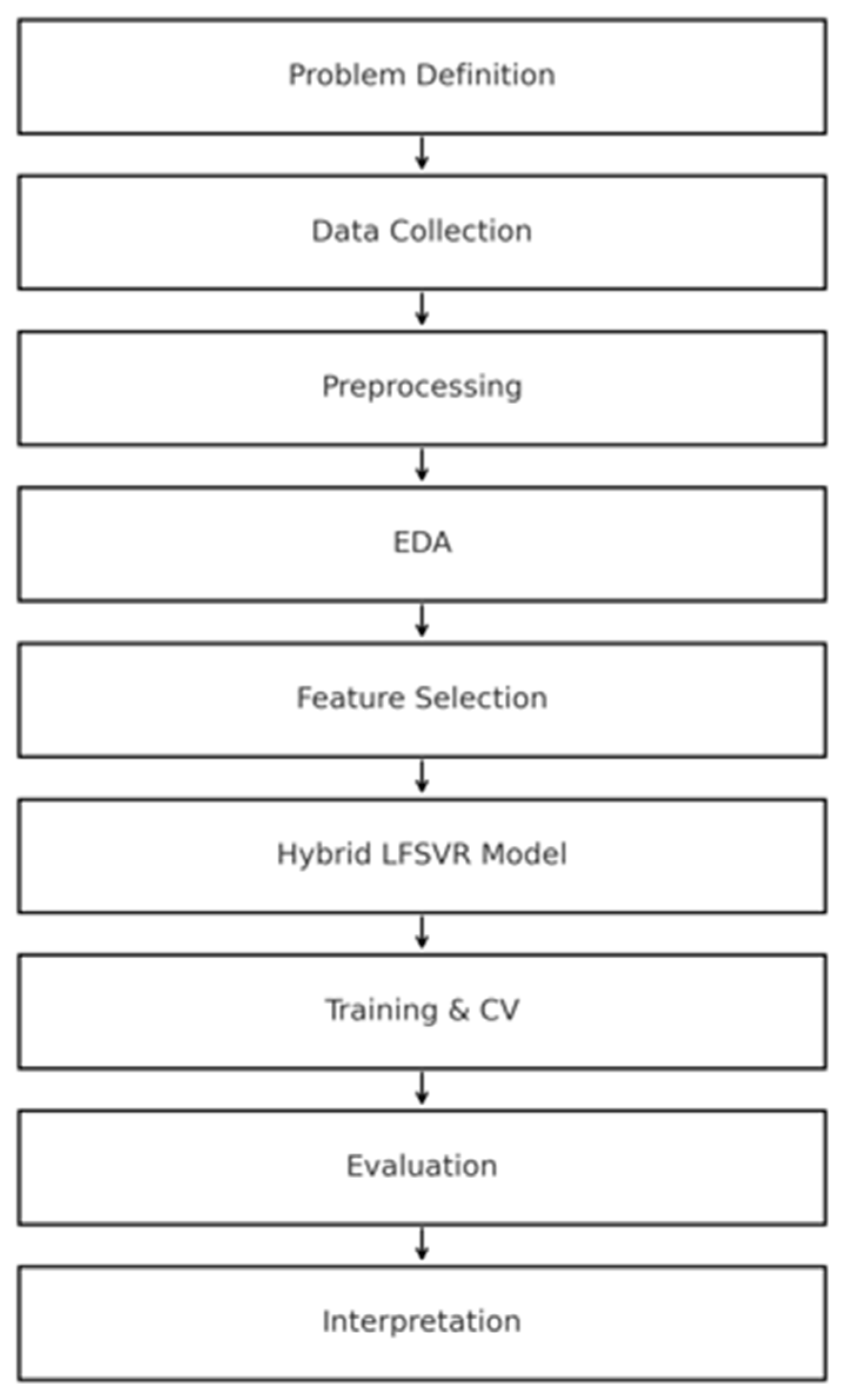
Figure 1. Hybrid model framework for LFSVR.
Agriculture 16 00065 g001
Figure 2. Comparative test-set performance of LR (R2 = 0.271) and RF (R2 = 0.143).
Agriculture 16 00065 g002
Figure 3. Exploratory Analysis of Yield Distribution Temporal Trends and Agroclimatic Relationships.
Agriculture 16 00065 g003
Figure 4. Temporal and Regional Stratification of Training and Test Sets.
Agriculture 16 00065 g004
Figure 5. Comparative test-set performance of RF (R2 = 0.271) and SVR (R2 = 0.143).
Agriculture 16 00065 g005
Figure 6. Diagnostic evaluation of the LFSVR hybrid model on the independent test set.
Agriculture 16 00065 g006
Table 1. Test-Set Performance of RF and SVM.
MethodRMSEMAE R 2
RF0.2680.1460.271
SVM0.2910.1490.143
Disclaimer/Publisher’s Note: The statements, opinions and data contained in all publications are solely those of the individual author(s) and contributor(s) and not of MDPI and/or the editor(s). MDPI and/or the editor(s) disclaim responsibility for any injury to people or property resulting from any ideas, methods, instructions or products referred to in the content.