Estimating Pruning Wood Mass in Grapevine Through Image Analysis: Influence of Light Conditions and Acquisition Approaches

Abstract

Pruning wood mass is crucial for grapevine management, as it reflects the vine’s vigor and balance. However, traditional manual measurement methods are time-consuming and labor-intensive. Recent advances in digital imaging offer non-invasive techniques, but limited research has explored pruning wood weight estimation, especially regarding the use of artificial backgrounds and lighting. This study assesses the use of image analysis for estimating wood weight, focusing on image acquisition conditions. This research aimed to (i) evaluate the necessity of artificial backgrounds and (ii) identify optimal daylight conditions for accurate image capture. Results demonstrated that estimation accuracy strongly depends on the sun’s position relative to the camera. The highest accuracy was achieved when the camera faced direct sunlight (morning on the northwest canopy side and afternoon on the southeast side), with R² values reaching 0.90 and 0.93, and RMSE as low as 44.24 g. Artificial backgrounds did not significantly enhance performance, suggesting that the method is applicable under field conditions. Leave-One-Group-Out Cross-Validation (LOGOCV) confirmed the model’s robustness when applied to Catarratto cv. (LOGOCV R² = 0.86 in NB and 0.84 in WB), though performance varied across other cultivars. These findings highlight the potential of automated image-based assessment for efficient vineyard management, using minimal effort adjustments to image collection that can be incorporated into low-cost setups for pruning wood weight estimation.

1. Introduction

Pruning wood mass plays a fundamental role in the management of grapevines (Vitis vinifera L.). Being considered for growth–yield relationship and used in the Ravaz Index as an indicator of vine balance, pruning wood weight is a key factor that can be used to achieve higher fruit quality, consistent production, and satisfying oenological results [1,2,3,4,5]. By adjusting pruning practices based on wood mass, vine potential can be evaluated, and various aspects can be regulated. These include the production of fertile shoots, and the number and size of the clusters, thus enabling crucial yield regulation in Wine Appellation circumstances, the maintenance of a vegetative and productive balance, and the reduction of the need for summer pruning. All of these aspects can promote grape quality, shoot lignification, reserves accumulation, and deeper root development. Additionally, they help control long-term productivity and contain production costs [6,7,8,9]. Moreover, pruning assists in achieving a balanced canopy structure and improved air circulation, which reduces the risk of pest infestations and fungal diseases [10]. Additionally, agronomical practices involving pruning residue burial as a sustainable tool to enhance soil nitrate availability also benefit from accurate assessment of the pruning mass [11]. At times, the process of manually measuring the pruning wood weight can be time-consuming due to the need for separating canes belonging to individual vines, as well as for interrupting the natural flow of the pruning work with the task of stacking, weighing, and recording the pruned wood [12]. Due to the influence of multiple factors, such as soil depth, slope, fertility, and agronomic practices, pruning wood assessment is essential for understanding the variability of a vineyard allowing for its effective management [13]. Non-destructive techniques capable of acquiring these data could bring benefits to both researchers and wine growers in quantifying spatial variability in terms of vigor and subsequent fruit quality and production [14,15,16,17]. These benefits include enabling selective operations such as targeted harvesting, a more efficient use of inputs, and overall vineyard precision management [18]. For this reason, the implementation of cost-reducing methods and procedures are needed [19,20]. In recent years, image analysis has risen as a promising technique for non-invasive phenotyping of plants and evaluation of yield components [21]. Moreover, the introduction of affordable digital cameras, larger hard-drive storage capacities, and advances in image-processing technology has been fundamental in helping to facilitate the advancement of this field [22]. Various methods have been proposed for the development of digital imaging and computer vision in viticulture. These approaches include classical RGB image processing techniques, such as segmentation, shape recognition, and feature extraction algorithms, which are defined to specific tasks. Examples include estimation of yield components, such as number of berries per bunch [23,24,25], number of flowers per inflorescence [18,26,27], or bunch number and weight [28,29,30,31,32,33]. Other authors proposed semi-automated or automated methods for canopy vigor and porosity assessment [34,35,36,37], for pruning automatization using mobile platforms and proximal sensors [38,39,40,41], or for berry quality components detection via proximal and remote sensing [42,43].

However, only a few studies have assessed pruning wood weight using image analysis, excluding UAV platforms and LiDAR sensors [13,44,45,46]. Some authors [47] experimented with a semi-automatic approach directly in the field without artificial backgrounds, using an extended prototype image acquisition system (PIAS) equipped with a complex multicamera system to acquire and analyze RGB images, achieving an R² = 0.44 in the relationship between the number of pixels segmented as pruned wood and the actual wood weight on ungrafted grapevine seedlings. Other authors [48] achieved promising results employing computer-based analysis of RGB images captured manually and on-the-go within a VSP Tempranillo vineyard, using a background and artificial illumination at night, obtaining an R² = 0.92 on manually captured vine images and an R² = 0.77 on on-the-go acquired images, and thus confirming the capability of this methodology to predict the pruning wood weight using cheap cameras and map the variability of the vine pruning weight.

Little research has explored the challenges of working without artificial backgrounds and the effects of varying daylight conditions, which are critical factors for adapting image analysis techniques to vineyard-level processes. Addressing these challenges could significantly improve the scalability and practicality of such methods for growers and researchers [32,49,50]. The hypothesis underlying this study was that vine image segmentation could be simplified by enhancing the scene’s conditions without introducing artificial modifications. To explore this, three lighting conditions commonly encountered in field conditions during image acquisition were identified. Additionally, an effort was made to replicate the uniformity typically achieved with an artificial background by angling the camera to ensure that the sky served as the sole background element. By incorporating these strategies, it could be possible to improve the accuracy and efficiency of assessing wood weight, enabling more informed decisions in vineyard management [23,25,28]. In light of this, the aims of the present study are as follows: (i) to overcome the limitations associated with using an artificial background, considering future process automation at the farm level; and (ii) to identify the suitable daylight conditions for image acquisition and analysis. By addressing these objectives, this work aims to enhance the efficiency and effectiveness of image analysis, providing valuable insights for researchers.

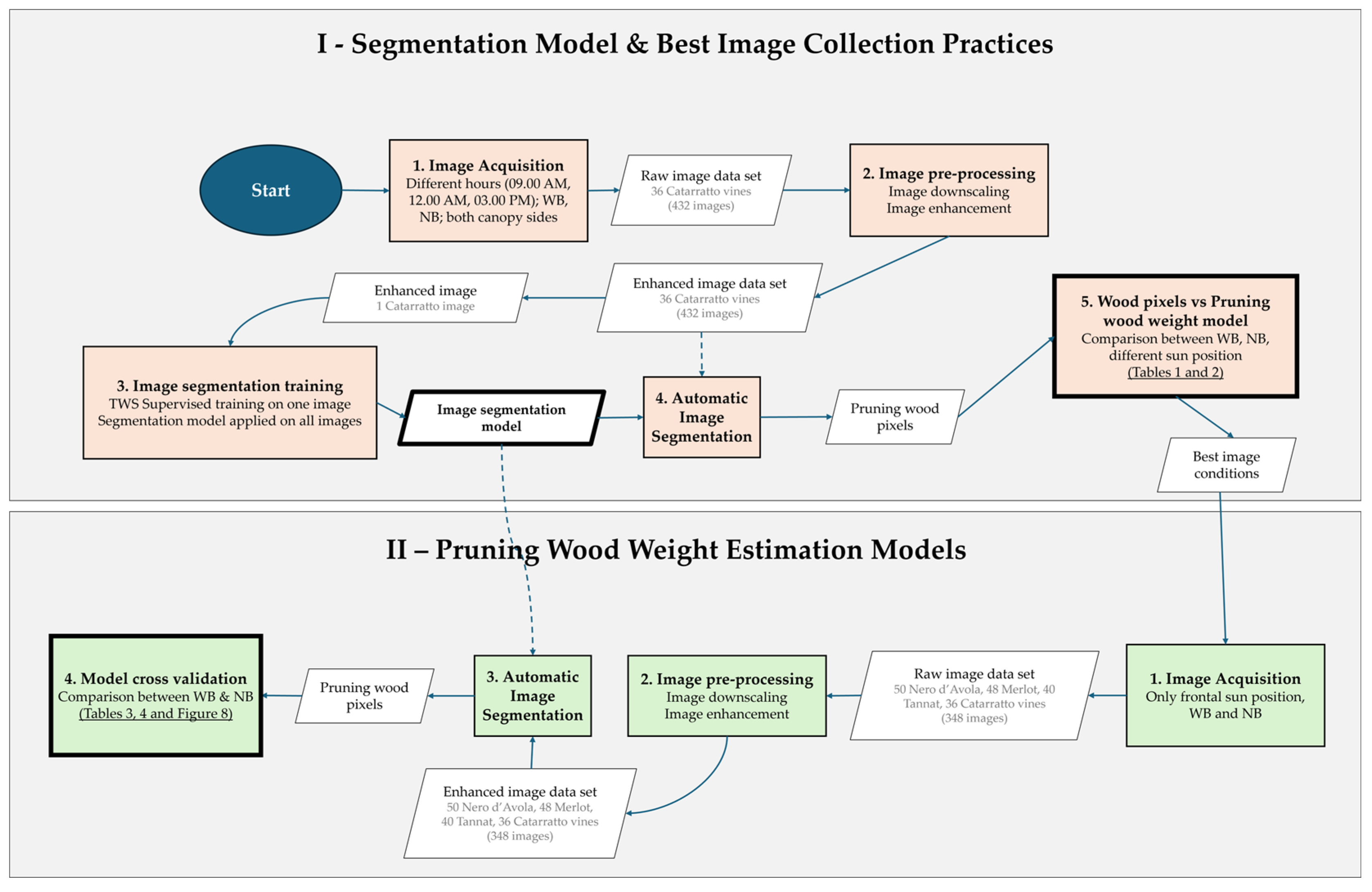
2. Materials and Methods

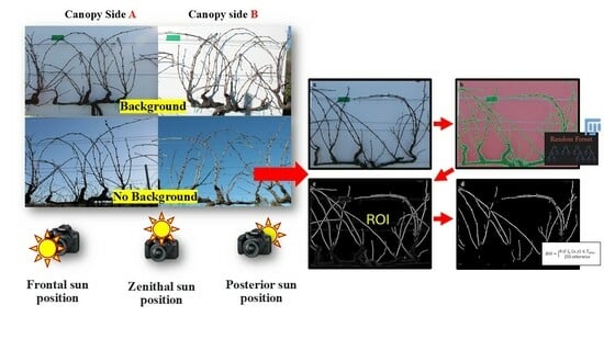
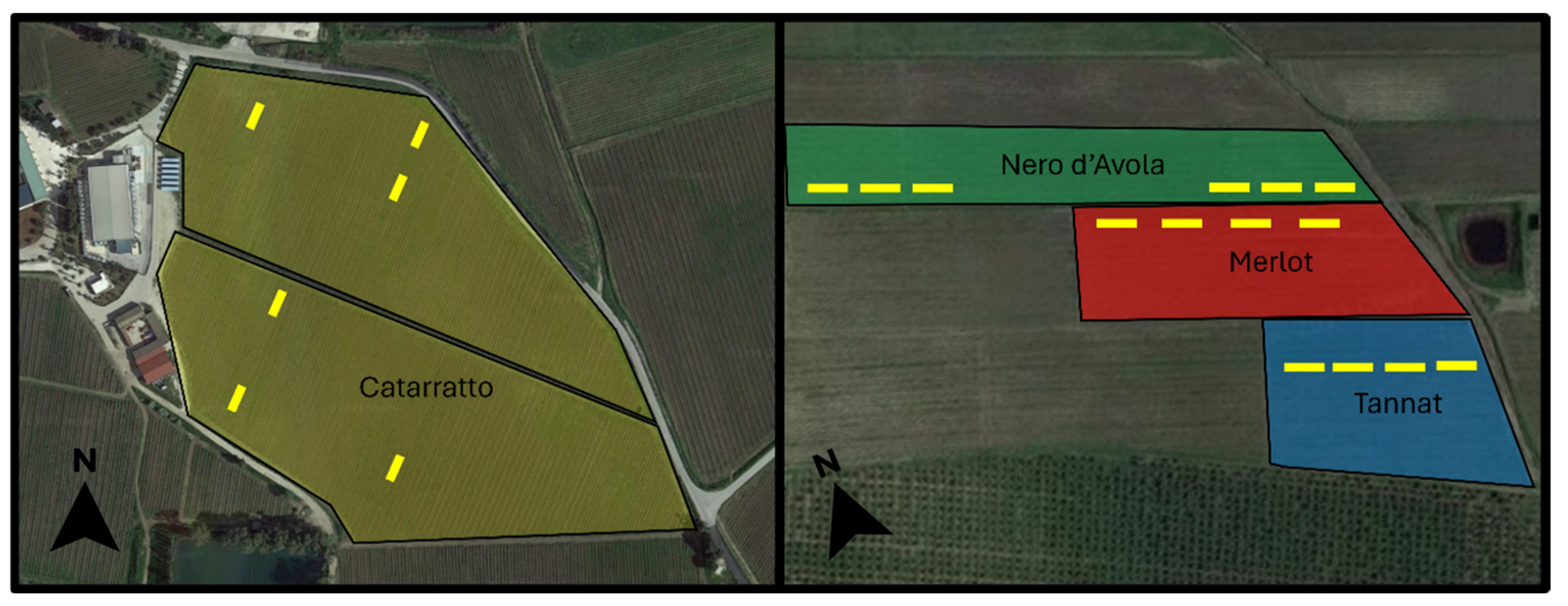
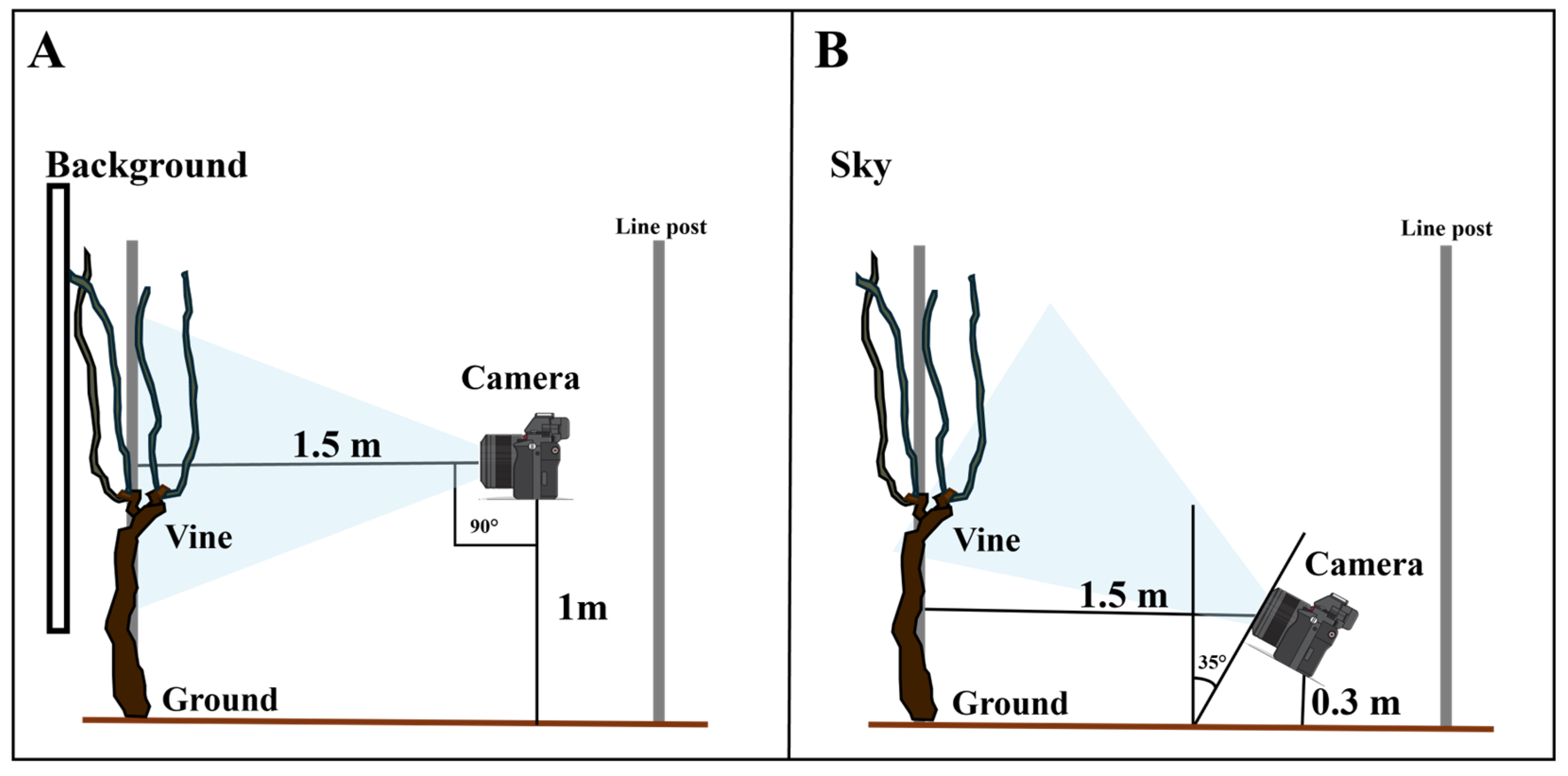
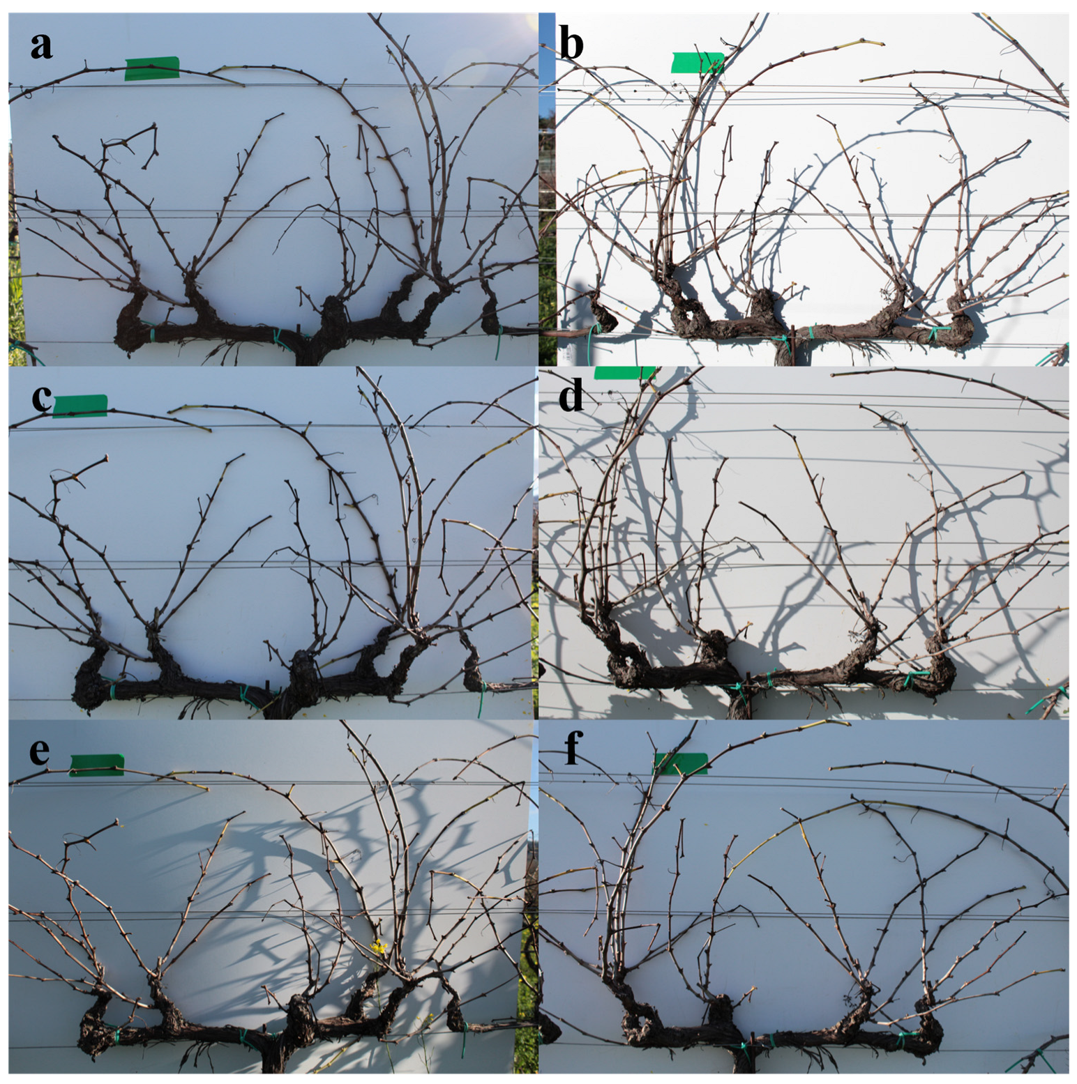
2.1. Experimental Design and Image Acquisition

Image acquisition was carried out between December 2022 and January 2023, before winter pruning, in four commercial vineyards of Catarratto, Nero d’Avola, Merlot, and Tannat cultivars (Vitis vinifera L.), grafted onto 1103P. Catarratto vineyard was located in Camporeale (37°55′12.82″ N, 13°04′28.33″ E; 320 m a.s.l.; Palermo, Italy). Vines were trained to a vertically shoot positioned (VSP) trellis system; pruned to double cordon; and spaced 0.9 m in rows and 2.2 m between rows, with northeast–southwest row orientation. Nero d’Avola, Merlot and Tannat vineyards were located in Santa Margherita Belice (37°40′47.93″ N; 13°04′28.96″ E; 252 m a.s.l.; Agrigento, Italy). All vines were trained to a vertically shoot positioned (VSP) trellis system pruned to single cordon and spaced 0.9 m in rows and 2.5 m between rows, with northwest–southeast row orientation. All four vineyards were drip-irrigated. Between each vineyard, a total of 174 vines were randomly selected to cover a wide range of pruning weight and occlusion conditions (36 vines of Catarratto, 50 of Nero d’Avola, 48 of Merlot, and 40 of Tannat).

The images of the vines were manually acquired using a Canon 1300D digital single-lens reflex camera equipped with an 18–55 mm f/3.5–5.6 DC Canon lens (Canon, Tokyo, Japan). The camera was configured with a sensitivity of ISO 400, an aperture of f/5.6, and a focal length of 24 mm. The exposure time was automatically selected. To define the best daylight condition and acquisition modality, a pilot test was conducted on the 36 vines of Catarratto cultivar, incorporating variability in light and acquisition setups (Figure 1).

Vines were photographed on both sides of the canopy (called A and B) under two acquisition modalities: (i) the camera was positioned directly perpendicular to the vine row, 1.5 m from the vines and 1 m above the ground, and a white board was used for background homogenization (with background—WB); and (ii) the camera was positioned 1.5 m from the vines with a 35° tilt angle from the ground to obtain images with the sky as homogeneous background (no background—NB) (Figure 2).

These acquisition modalities accounted for the variability caused by adjacent vines and aimed to evaluate the influence of background elements on segmentation accuracy. The same images were acquired under three different light conditions: (a) the sun was in front of the operator and directed toward the camera lens (approximately 09:00 a.m.); (b) the sun was at its zenith (approximately 12:00 a.m.); (c) the sun was behind the operator (approximately 03:00 p.m.) and directed toward the vines and the white background, in the case of with background (WB) (Figure 3 and Figure 4). Despite being taken at the same time of day, sunlight affects the images differently: in (b), shadows are cast on the background due to the sun’s position behind the camera, while in (d), variations in color occur among pixels representing the shoots. Conversely, in (a) and (c), where the sun is in front of the camera, higher contrast results in greater uniformity. The image acquisition protocol was designed for sunny or partly cloudy conditions, as these present the most challenging lighting scenarios due to direct sunlight and the presence of cast shadows. Images were taken at three different times of the day and on both canopy sides to account for variations in sun position relative to the camera. In fully overcast conditions, light diffusion minimizes shadow artifacts, making segmentation easier.

After image analysis and model evaluation, Nero d’Avola, Merlot and Tannat images were acquired under a single daylight condition (the one where the best results were obtained for the Catarratto pilot test) on each acquisition modality (Figure 5). Subsequently, after image acquisition, vines were pruned, and pruning wood weight was measured using a digital gauge for the ground-truthing process.

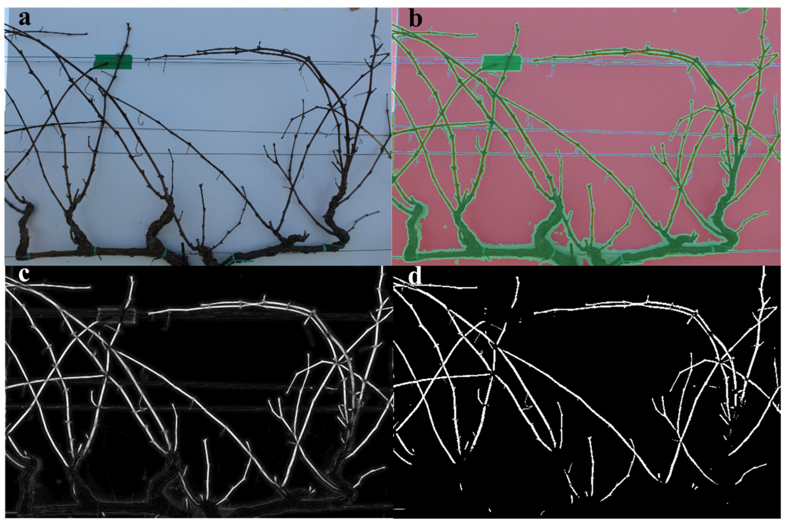
2.2. Image Analysis for Pruning Weight Assessment

Acquired images were pre-processed and analyzed using the open-source FIJI/ImageJ^® version 1.53c software and its Trainable Weka Segmentation (TWS) plug-in [51]. The TWS plug-in employs a combination of image segmentation and machine learning algorithms to classify red–green–blue or grayscale image pixels into different classes based on similar visual characteristics, such as color, shape, and texture. It uses machine learning algorithms for data mining tasks. It was developed at Waikato University in New Zealand and is a well-known workbench for data mining using machine learning [51,52]. The image acquisition, processing, and data analysis stages are illustrated in Figure 6.

First, since the training, segmentation, and measurement process speed can be affected by image resolution, all images were downscaled from 5184 × 3456 to 1773 × 1182 pixels using bicubic interpolation to ensure smooth transitions and better preservation of fine details. Then, all images were uploaded in FIJI/Imagej^® to manually remove the adjacent vines within the same row to the one under study using the Pencil tool. This step aims to prevent their canes and shoots from interfering with the scene and to avoid affecting the precision of the ground-truthing process. Following that, Trainable Weka Segmentation was activated (plug-ins > segmentation > Trainable Weka Segmentation) and, still within the image pre-processing task, the following functions were used in default mode [53]: Gaussian blur to smooth the image; Sobel filter to capture the edges in the image; Hessian to capture the shape of objects; difference of Gaussians to highlights edges and other details in the image that vary in size; membrane projections to enhance the contrast along the boundary; and FastRandomForest, a decision tree algorithm that builds a tree of “if-then” rules to classify image pixels based on the color, shape, and texture similarities. Prior to segmentation, the TWS plug-in requires a supervised segmentation by manually training the classifier with traces or sets of training pixels (STPs) over the region of interest (ROI) for each class. For the training process, one image per acquisition modality from the dataset was selected and used as a sample. Four classes were defined within the image (pruning wood, trunk and cordon, trellis wires, and background) by manually drawing ten free-hand lines for each class (approximately 50 pixels length and 1 pixel width). The training process yielded a stack of four images (one per class) encompassing all the manually selected lines (see Supplementary Materials). Subsequently, the segmentation model was applied to all images in the dataset by stacks of six images at a time. The images obtained as a result of the TWS segmentation were turned into a single stack containing only the class for the ROI. This stack was converted to 8-bit and then transformed into the binary format to reduce the amount of information (image > type > 8-bit). Next, the region of interest (ROI), i.e., pruning wood, was extracted from the image by automatic thresholding of the b* channel of the CIELAB color space using Otsu’s method [54]. This method calculates the optimal T_otsu threshold for a grayscale image by assuming the existence of two classes of pixels, related to the background and foreground, and maximizing their variance to include them in one of the two classes. If I_b represents a grayscale image, b*, as a two-dimensional function in discrete space whose values fall in the interval [0, ..., 255], then the following applies:

$$ROI=\left\{\begin{array}{c}0if{I}_b\left(x,y\right)\le T_{otsu}\\ 255otherwise\end{array}\right.$$

(1)

This yields a binary image (0 = white; and 255 = black) containing only the ROI and background pixels (image > adjust > auto-threshold). The ROI pixel number was then measured using the Measure tool and turned into a percentage of black pixels in a frame of 1773 × 1182 pixels. The flowchart of the main steps for estimating pruning wood weight is shown in Figure 7.

2.3. Statistical Analysis and Models Evaluation

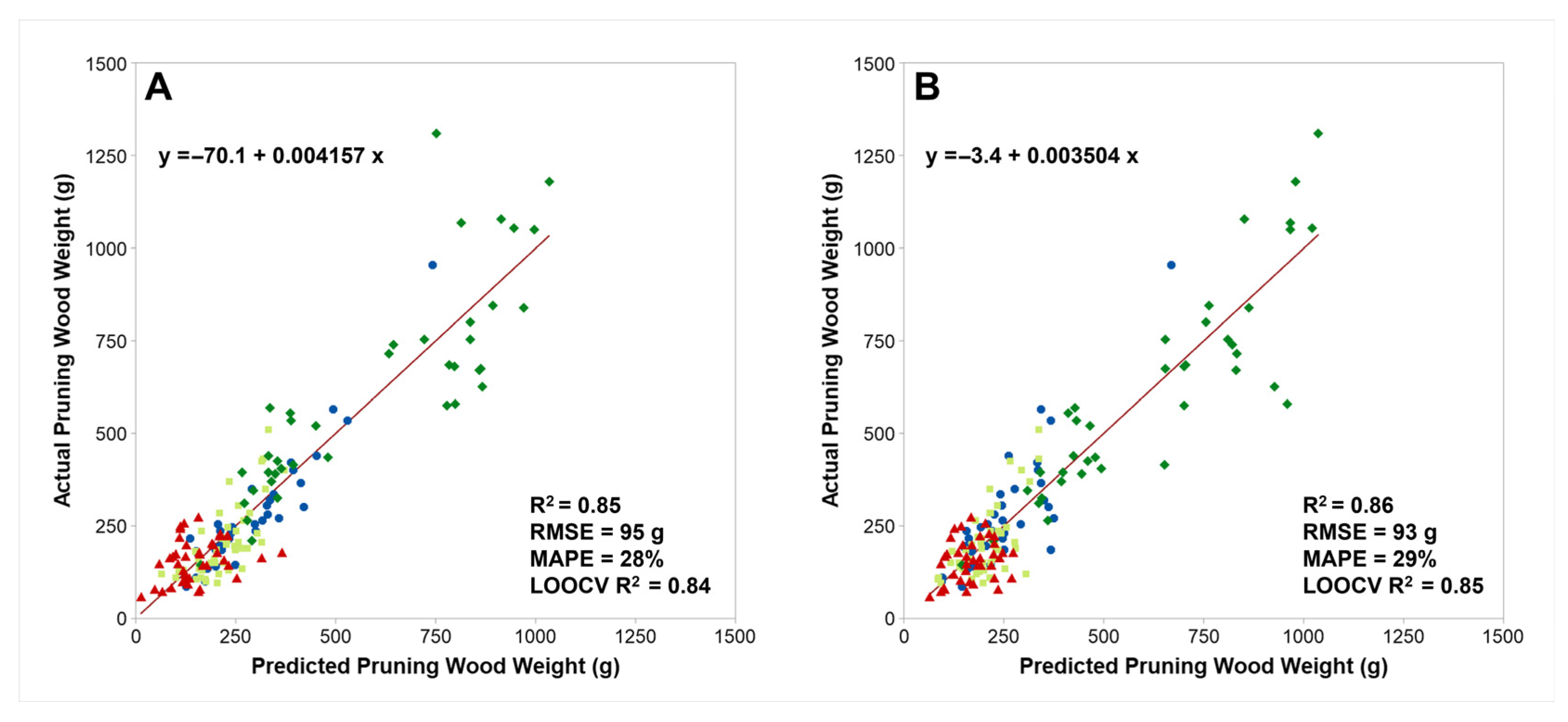
The data obtained from the image processing and their relationship to reference ground-truthing values were analyzed using the statistical software Minitab^® version 17 (Minitab, Inc., Philadelphia, PA, USA). Regression lines, along with their coefficient of determination (R²), 95% confidence intervals of the slope coefficients, and p-values, were calculated. To quantify the absolute magnitude of the prediction errors, models were evaluated using Root Mean Square Error (RMSE) and Mean Absolute Percentage Error (MAPE), as described by [55], using the following equation:

$$RMSE=\sqrt{mean{(t-a)}^2}$$

(2)

$$MAPE=mean\left(\left|{\displaystyle \frac{t-a}{t}}\ast 100\right|\right)$$

(3)

where t (target) is the predicted value, and a (actual) the actual value.

The Akaike Information Criterion (AIC) and Bayesian Information Criterion (BIC) were also calculated. Additionally, Leave-One-Out Cross-Validation (LOOCV) and Leave-One-Group-Out Cross-Validation (LOGOCV) were performed.

3. Results

This study investigated the relationship between the number of pixels extracted from images as pruning wood and the actual weight of pruning assessed in the vineyard, according to different acquisition modes and light conditions. The aim was to determine the best combination that would allow for more accurate segmentation and estimation. The automatic segmentation process made it possible to exclude from the images the elements related to trunk and cordons, structure support wires, and background (natural or artificial) without requiring manual intervention; it was necessary only to exclude elements correctly segmented but belonging to contiguous plants. The segmentation process took about twenty seconds per image. The performance of the linear models for each combination of acquisition time, sun position, and canopy side in both WB and NB modes is summarized in

Table 1. Summary of linear models’ performance for each combination of acquisition time, sun position relative to the camera, and canopy side, from images acquired with the presence of artificial background (WB) on Catarratto cv.

Time (±1 h)	Canopy Side	Sun Position	p-Value	R2	RMSE (g)	MAPE	AIC	BIC	LOOCV R2
09.00 a.m.	A	Frontal	0.00	0.84	66.57	18.61	409.13	413.13	0.77
	B	Behind	0.00	0.30	138.25	41.00	461.75	467.75	0.16
12.00 a.m.	A	Top	0.00	0.69	91.34	22.54	431.91	435.91	0.58
	B	Top	0.00	0.42	125.23	33.83	454.63	458.63	0.27
03.00 p.m.	A	Behind	0.00	0.27	141.25	44.34	463.32	467.32	0.09
	B	Frontal	0.00	0.89	55.80	15.74	396.42	400.42	0.84

R², coefficient of determination; RMSE, Root Mean Square Error; MAPE, Mean Absolute Percentage Error; AIC, Akaike Information Criterion; BIC, Bayesian Information Criterion; LOOCV R², coefficient of determination of Leave-One-Out Cross-Validation. N = 36.

and

Table 2. Summary of linear models’ performance for each combination of acquisition time, sun position relative to the camera, and canopy side from images acquired without the presence of artificial background (NB) on Catarratto cv.

Time (±1 h)	Canopy Side	Sun Position	p-Value	R2	RMSE (g)	MAPE	AIC	BIC	LOOCV R2
09.00 a.m.	A	Frontal	0.00	0.90	51.75	17.41	391.00	395.00	0.86
	B	Behind	0.00	0.32	136.54	40.67	460.85	464.58	0.17
12.00 a.m.	A	Top	0.00	0.74	83.60	22.10	425.54	429.54	0.62
	B	Top	0.00	0.48	118.40	33.01	450.59	454.59	0.32
03.00 p.m.	A	Behind	0.00	0.33	135.00	43.59	460.02	464.02	0.11
	B	Frontal	0.00	0.93	44.24	16.62	379.70	383.71	0.92

R², coefficient of determination; RMSE, Root Mean Square Error; MAPE, Mean Absolute Percentage Error; AIC, Akaike Information Criterion; BIC, Bayesian Information Criterion; LOOCV R², coefficient of determination of Leave-One-Out Cross-Validation. N = 36.

, highlighting the impact of lighting conditions on estimation accuracy.

For the WB mode, morning measurements showed significant differences between the northwest (A) and southeast (B) sides of the canopy in terms of model performance. Side A, where the camera faced the sun, exhibited the highest accuracy (R² = 0.84; RMSE = 66.57 g), while side B, where the sun was behind the camera, had lower precision (R² = 0.30; RMSE = 138.25 g). At midday, when the sun was positioned directly above the canopy, side A retained a higher R² (0.69) compared to side B (0.42), though both showed moderate estimation errors (RMSE = 91.34 g and 125.23 g, respectively). In the afternoon, the accuracy patterns were inverted compared to the morning: side A, now with the sun behind the camera, had the lowest R² (0.27) and the highest estimation error (RMSE = 141.25 g), whereas side B, which now faced the sun, achieved the best accuracy among all cases studied (R² = 0.89; RMSE = 55.80 g) (Table 1). In accordance with the lowest BIC, AIC, and MAPE values, the best-performing models were those corresponding to the frontal position of the sun at 09:00 a.m. and 03:00 p.m.

Similar trends were observed in the NB mode, with the highest accuracy occurring when the sun was positioned in front of the canopy side being captured. Morning acquisitions showed a high R² for side A (0.90; RMSE = 51.75 g) and lower precision for side B (R² = 0.32; RMSE = 136.54 g). At midday, both sides showed moderate accuracy (side A: R² = 0.74 and RMSE = 83.60 g; side B: R² = 0.48 and RMSE = 118.40 g). In the afternoon, side A had a low R² (0.33) and high RMSE (135.00 g), while side B, which was frontal to sunlight, had the highest overall accuracy across all cases (R² = 0.93; RMSE = 44.24 g) (Table 2). Other model performance indicators, such as MAPE, AIC, and BIC, followed similar relative trends.

After identifying the best illumination conditions (morning images of side A and afternoon images of side B) the full dataset (with all four cultivars) was used to model the relationship between pruning wood pixels and pruning weight on both WB and NB modes. Other model options were tested to explore this relationship (quadratic and polynomial regression) with no significant or inexistant improvements when compared to a linear regression or with high Variance Inflation Factor values. Thus, for parsimony reasons, the linear model was selected. Although machine learning methods were considered, we opted for regression models that provide greater interpretability and robustness in this context. Given the structured nature of our dataset, lower-complexity models were considered more suitable for effectively capturing the relationships between variables. To assess the generalizability of the models across different cultivars, Leave-One-Group-Out Cross-Validation (LOGOCV) was performed, with results presented in

Table 3. Leave-One-Group-Out Cross-Validation results for model performance from images acquired with the presence of artificial background (WB) on Catarratto cv.

Training Set	Validation	n	p-Value	R2	RMSE (g)	MAPE	AIC	BIC
Merlot, Nero d’Avola, Tannat	Catarratto	36	0.00	0.73	85.95	26.26	427.53	431.53
Catarratto, Nero d’Avola, Tannat	Merlot	48	0.00	0.44	74.01	32.93	553.93	559.00
Catarratto, Merlot, Tannat	Nero d’Avola	40	0.00	0.78	131.96	15.15	496.14	500.45
Catarratto, Merlot, Nero d’Avola	Tannat	40	0.13	0.06	56.46	36.90	440.82	445.22

R², coefficient of determination; RMSE, Root Mean Square Error; MAPE, Mean Absolute Percentage Error; AIC, Akaike Information Criterion; BIC, Bayesian Information Criterion.

and

Table 4. Leave-One-Group-Out Cross-Validation results for model performance from images acquired without the presence of artificial background (NB) on Catarratto cv.

Training Set	Validation	n	p-Value	R2	RMSE (g)	MAPE	AIC	BIC
Merlot, Nero d’Avola, Tannat	Catarratto	36	0.00	0.89	55.8	15.74	396.42	400.42
Catarratto, Nero d’Avola, Tannat	Merlot	48	0.00	0.55	66.23	27.46	543.26	548.33
Catarratto, Merlot, Tannat	Nero d’Avola	40	0.00	0.72	150.66	18.19	506.26	510.56
Catarratto, Merlot, Nero d’Avola	Tannat	40	0.05	0.09	55.46	36.55	493.38	443.78

R², coefficient of determination; RMSE, Root Mean Square Error; MAPE, Mean Absolute Percentage Error; AIC, Akaike Information Criterion; BIC, Bayesian Information Criterion.

.

The results from the Leave-One-Group-Out Cross-Validation for model performance on the four cultivars show varying levels of accuracy depending on the presence of an artificial background (WB) or not (NB). In WB, the R² values range from 0.06 to 0.78, with the highest value (0.78) when training with Catarratto, Merlot, and Tannat to predict Nero d’Avola, and the lowest (0.06) when training with Catarratto, Merlot, and Nero d’Avola to predict Tannat. RMSE values also indicate more significant prediction errors for some validation sets, with the highest error (131.96 g) in the Catarratto, Merlot, and Tannat to Nero d’Avola prediction. MAPE shows a similar trend, with the best accuracy (15.15%) for predicting Nero d’Avola and the worst (36.90%) for Tannat. The AIC and BIC values are lowest for the prediction of Catarratto from Merlot, Nero d’Avola, and Tannat (AIC = 427.53; BIC = 431.53), indicating the most balanced model. In NB, R² values generally improve, with the highest value (0.89) when predicting Catarratto from Merlot, Nero d’Avola, and Tannat, and the lowest (0.09) when predicting Tannat from Catarratto, Merlot, and Nero d’Avola. The RMSE values are also lower for NB, with the best result (55.8 g) when predicting Catarratto from the same varieties. The MAPE values show better accuracy as well, with the lowest (15.74%) for the prediction of Catarratto. AIC and BIC values are again lowest for the Catarratto prediction (AIC = 396.42; BIC = 400.42), supporting the better performance of the NB models. Overall, the models perform better with images without artificial background, with the best prediction accuracy occurring for Catarratto, while the Tannat predictions remain the least accurate in both cases. The AIC and BIC values further emphasize the better fit of the models trained with the NB images.

Scatter plots of actual vs. predicted wood weight in the WB and NB modes were similar. The regression models (Figure 8) among the four cultivars that had a significant correlation between pixels and wood weight show that, regardless of the use of artificial background, the estimation accuracy is similar for the two acquisition modes: an R² of 0.84 for the WB mode and 0.85 for the NB mode after LOOCV, with an RMSE of 95 and 93 g and a MAPE of 28 and 29%, respectively.

4. Discussion

The following study contributes to accrediting the possibility of using image analysis to estimate pruning wood weight, a useful parameter for monitoring vegetative balance and variability in vineyards, without resorting to destructive methods. As found in other studies supporting such possibilities, one of the main limitations related to this need in outdoor conditions is the influence of lighting conditions and the need to use backgrounds or artificial illumination.

The use of an artificial background helps create a controlled image acquisition environment, making it easier to segment and analyze targeted plant parts, such as grape clusters, canes, or leaves. Similarly, artificial lighting enhances image quality, color contrast, and feature extraction algorithms. However, these methods may not be practical or feasible for on-farm applications, as they hinder expedite data collection; meanwhile, not using them can create diverse challenges, as vineyards are characterized by diverse lighting conditions and non-homogeneous backgrounds [23,25,28]. In this study, we evaluated the impact of different lighting conditions throughout the day on the acquired images and explored the elimination of the artificial background by adjusting the camera angle. The accuracy of the estimation can change depending on the position of the sun relative to the camera and the presence of disruptive objects within the image. As shown in Figure 4, one of the main variables influencing the quality of the images and, therefore, the estimation, was the shadow cast by the shoots on other objects within the image. In fact, where the image had excessive variations in terms of color and texture for the same class (e.g., “pruning wood”), an overestimation of the weight of the wood was observed. This occurred when the sun was behind the camera (regardless of WB or NB cases), in the afternoon (3:00 p.m.) for canopy side A and in the morning (9:00 a.m.) for canopy side B. In these cases, the shadows cast on the background were perceived as disturbances, and the automatic segmentation algorithm identified them as real shoots. For this reason, determining the optimal image acquisition conditions—such as the time of day and camera positioning—can help reduce noise and facilitate easier segmentation with minimal effort and cost. On the contrary, when the sun was in front of the operator (in the morning, on side A; and in the afternoon, on side B), images were obtained with better contrast, which made the shoots stand out against the background, thus improving the segmentation process by creating more uniform pixels in terms of color.

Having established the most effective acquisition modality for segmentation on the Catarratto cultivar, the same process was applied to images of other cultivars, namely Nero d’Avola, Tannat and Merlot, creating a single dataset for both WB and NB modalities (Figure 5). The results of this approach show that it is possible to dispense with the artificial background and still achieve reliable pruning weight estimates, without the need for specialized equipment other than a camera mounted on a vehicle performing regular vineyard tasks, as highlighted by other authors [48]. Regardless of whether the artificial background was used, the segmentation process yielded similar results in terms of the accuracy of wood weight estimation, suggesting that this acquisition method can be effectively applied in the field without adding complexity to the system.

One of the main challenges in applying this methodology, as observed in this study, is occlusion. Occlusion refers to when parts of the grapevine shoots or canes are hidden or obscured by other shoots, making it difficult to accurately determine their dimensions or weight. Occlusion can occur due to the natural growth pattern of grapevines, where shoots overlap each other, or due to the increase in density as the vine’s vigor increases. In addition, where shoots tend to grow procumbently, causing mutual overlap, this results in an image in which the shoot pixels are inevitably underestimated. To further investigate the impact of occlusion, the number of shoot overlaps was manually identified in each image for the Catarratto variety. This indicator showed a strong correlation with pruning weight (r = 0.85), suggesting that higher pruning mass tends to result in increased occlusion. This result aligns with expectations, as higher pruning weight generally leads to increased shoot density and, consequently, a greater likelihood of occlusion. However, when comparing this indicator with estimation error, no significant correlation was found (r ≈ 0), suggesting that within the pruning weight range of our dataset, the method remains reliable regardless of occlusion magnitude. Despite these findings, it is important to acknowledge that extreme occlusion scenarios, particularly in highly vigorous vineyards with dense shoot growth, could still introduce estimation biases, which are not addressed in this work. The issue of occlusion is common when using image-based methods to estimate the mass or number of other grapevine organs [28], such as shoots at an early stage [28,56], inflorescences [57], and clusters [58]. However, particularly regarding inflorescences and clusters, occlusion can reach magnitudes up to 90% [23], which is significantly different from when leaves are no longer present in the vine, as is the case of the pruning weight. One other challenge of the current methodology is the natural variability in shoot positioning regarding the camera. Although the distance between the camera and the plants remained constant, the shoots themselves were not perfectly straight, leading to small variations in their actual distance from the camera. These variations could result in slight underestimation or overestimation of pruning wood weight. Additionally, another contributing factor to estimation error is the variability in wood density, which can fluctuate depending on the amount of stored starch [59]. This intrinsic variability in shoot structure and composition may overshadow the error introduced by occlusion, making its direct effect on estimation accuracy less apparent.

In Kicherer et al. [47], authors evaluated a set of 39 vines images taken without background under daylight conditions and found an R² of 0.84 and a RMSE of 0.12 g operating a manual segmentation, but only an R² of 0.44 and RMSE of 0.23 g operating with an automated depth segmentation because of the difficulty of the algorithm to identify vines featuring thin shoots and abundant tendrils. As they suggested, in our work, the problem was overcome by incorporating prior knowledge about the scene thanks to the definition of the four classes and adopting features that take into account more information from the RGB images, like color, to better distinguish between the foreground plant and the background. Other authors [48] operated on a set of 44 vines, obtaining an R² of 0.91, RMSE of 87.7 g, and MAE of 61.7 g, using an artificial background, but only a R² of 0.77, RMSE of 148 g and MAE of 147.9 g on nighttime acquired images without the use of background due to the uncontrolled background and the motion of the on-the-go acquisition. They also highlighted that the coefficient of determination decreased when the lower pruning weight vine values were removed. Increasing the variability within the sample in our 174-image set from different cultivars helped to obtain a solid result. This suggests that a larger dataset may contribute to obtaining a more stable model and highlights that the present methodology has the potential to generalize across different grapevine cultivars. This is an important step forward because, unlike previous studies [47,48], which did not specifically address cultivar variability, the present study suggests that cultivar can influence the relationship between pixel number and actual wood weight. In fact, one of the varieties used (Tannat), when used solely for validation in a Leave-One-Group-Out Cross-Validation, presented a low and non-significant R². Variety dependence is common in image-based modeling in the vineyard [25,60,61]; however, although the worse results were specific for one variety, it also coincided with the fact that this variety presented a much lesser magnitude of pruning weight variability.

The present research reveals highly competitive results when compared to other similar studies that use technologies such as Multispectral Imaging (R² = 0.88) [13], manual image segmentation (R² = 0.84) [47], LiDAR (R² = 0.91) [45], Backdrop Image Segmentation, Mahalanobis distance, and SVM classifiers (R² = 0.92 and 0.77) [48], Photogrammetry (R² = 0.62) [44], and low-cost structured light 2D and 3D imaging (R² = 0.80) [62]. In the present case, the cost associated with the methodology rivals the one presented by Jaramillo et al. [62], potentially being even cheaper, as it does not require for it to be performed during nighttime, thus not requiring artificial lighting. Additionally, the present methodology is capable of being associated with other activities in the vineyard if the imaging device is coupled with other machinery.

Considering the several handicaps that are still relevant in the topic of pruning weight estimation, further studies should apply the methodology to a larger number of cultivars, taking into consideration rootstock characteristics (vigor) and vegetative habitus, which can certainly contribute to very different occlusion conditions. Furthermore, while our methodology does not explicitly quantify light intensity, it considers variations in sunlight direction to ensure robustness across different times of day. Future studies could explore adaptive image enhancement techniques, such as histogram equalization, to further mitigate lighting variability. Future research should also focus on refining segmentation methods to better handle occlusion, potentially integrating depth information or machine learning techniques to improve segmentation accuracy in complex vineyard canopies. Additionally, developing a standardized occlusion index applicable to different vineyard conditions could further enhance model robustness and generalization. Furthermore, while our methodology does not explicitly quantify light intensity, it considers variations in sunlight direction to ensure robustness across different times of day. Future studies could also explore adaptive image enhancement techniques, such as histogram equalization, to further mitigate lighting variability.

5. Conclusions

This study contributes to validating image analysis as a viable tool for estimating pruning wood weight in vineyards, offering a non-destructive alternative for monitoring vegetative balance and variability. The findings highlight the potential of this method to be applied without the need for destructive measures and elaborate instrumentation, making it feasible for routine vineyard operations if coupled with platforms or vehicles that already move through the vineyard, such as tractors or autonomous robots.

The observed variations in image quality due to shadows and lighting conditions emphasize the importance of selecting an optimal acquisition modality for consistent and reliable results. Addressing the limitations associated with outdoor conditions, particularly variations in lighting, was a key focus of this research. Rather than developing a new segmentation method, this study emphasized optimizing the image acquisition setup, including the time of day and the tilted camera position, to eliminate the need for artificial backgrounds. The results demonstrated that flexible acquisition timing can accommodate different vineyard orientations, provided the sun remains behind the canopy, opposite to the camera, thereby reducing shadow interference and improving segmentation accuracy. This flexibility makes the approach adaptable to diverse vineyard setups and practical for large-scale applications. Differences in performance between varieties were clear, demonstrating that this system can generalize across different cultivars while accounting for potential variability. This highlights the potential for scaling this approach beyond the specific cultivars studied, enabling broader adoption across vineyard management systems.

The results indicate that, regardless of the use of artificial backgrounds, the segmentation process yielded comparable outcomes in terms of the accuracy of wood weight estimation. This finding underscores the practicality of dispensing with artificial backgrounds, thereby simplifying implementation to only require a camera mounted on routine vineyard vehicles or even a smartphone. Such simplicity makes this approach more accessible for widespread use in commercial vineyards, particularly when integrated into existing digital viticulture platforms. For example, this method could be paired with real-time data analytics, allowing vineyard managers to assess pruning weight distribution across the field and adjust canopy management strategies accordingly. Future research could focus on developing a fully automated version of this system, integrating it with AI-powered vineyard monitoring tools to enable real-time processing and decision support for pruning operations. Additionally, expanding the dataset to include a larger variety of cultivars and vineyard orientations will be essential for ensuring robustness. Furthermore, testing additional correction factors could further enhance the generalizability of the proposed methodology. By incorporating such improvements, this method could contribute to the development of a powerful, scalable tool for non-destructive vineyard monitoring, playing a crucial role in modern precision viticulture and sustainable vineyard management.

References

1. Petrie, P.R.; Trought, M.C.; Howell, G.S. Growth and Dry Matter Partitioning of Pinot Noir (Vitis vinifera L.) in Relation to Leaf Area and Crop Load. Aust. J. Grape Wine Res. 2000, 6, 40–45. [Google Scholar] [CrossRef]
2. Howell, G.S. Sustainable Grape Productivity and the Growth-Yield Relationship: A Review. Am. J. Enol. Vitic. 2001, 52, 165–174. [Google Scholar] [CrossRef]
3. Petrie, P.R.; Trought, M.C.; Howell, G.S. Fruit Composition and Ripening of Pinot Noir (Vitis vinifera L.) in Relation to Leaf Area. Aust. J. Grape Wine Res. 2000, 6, 46–51. [Google Scholar] [CrossRef]
4. Smart, R.; Robinson, M. Sunlight into Wine: A Handbook for Winegrape Canopy Management; Winetitles: Underdale, Australia, 1991. [Google Scholar]
5. Viala, P.; Ravaz, L. American Vines (Resistant Stock): Their Adaptation, Culture, Grafting and Propagation; Press of Freygang-Leary: Tokyo, Japan, 1908. [Google Scholar]
6. Tomasi, D.; Gaiotti, F.; Petoumenou, D.; Lovat, L.; Belfiore, N.; Boscaro, D.; Mian, G. Winter Pruning: Effect on Root Density, Root Distribution and Root/Canopy Ratio in Vitis vinifera Cv. Pinot Gris. Agronomy 2020, 10, 1509. [Google Scholar] [CrossRef]
7. Palliotti, A.; Poni, S.; Silvestroni, O. Manuale di Viticoltura; Edagricole: Bologna, Italy, 2018; ISBN 88-506-5533-9. [Google Scholar]
8. Poni, S.; Tombesi, S.; Palliotti, A.; Ughini, V.; Gatti, M. Mechanical Winter Pruning of Grapevine: Physiological Bases and Applications. Sci. Hortic. 2016, 204, 88–98. [Google Scholar] [CrossRef]
9. Kliewer, W.M.; Dokoozlian, N.K. Leaf Area/Crop Weight Ratios of Grapevines: Influence on Fruit Composition and Wine Quality. Am. J. Enol. Vitic. 2005, 56, 170–181. [Google Scholar] [CrossRef]
10. Calonnec, A.; Burie, J.B.; Langlais, M.; Guyader, S.; Saint-Jean, S.; Sache, I.; Tivoli, B. Impacts of Plant Growth and Architecture on Pathogen Processes and Their Consequences for Epidemic Behaviour. Eur. J. Plant Pathol. 2013, 135, 479–497. [Google Scholar] [CrossRef]
11. Pisciotta, A.; Di Lorenzo, R.; Novara, A.; Laudicina, V.A.; Barone, E.; Santoro, A.; Gristina, L.; Barbagallo, M.G. Cover Crop and Pruning Residue Management to Reduce Nitrogen Mineral Fertilization in Mediterranean Vineyards. Agronomy 2021, 11, 164. [Google Scholar] [CrossRef]
12. Taylor, J.A.; Bates, T.R. Comparison of Different Vegetative Indices for Calibrating Proximal Canopy Sensors to Grapevine Pruning Weight. Am. J. Enol. Vitic. 2021, 72, 279–283. [Google Scholar] [CrossRef]
13. Dobrowski, S.Z.; Ustin, S.L.; Wolpert, J.A. Grapevine Dormant Pruning Weight Prediction Using Remotely Sensed Data. Aust. J. Grape Wine Res. 2003, 9, 177–182. [Google Scholar] [CrossRef]
14. Santesteban, L.G. Precision Viticulture and Advanced Analytics. A Short Review. Food Chem. 2019, 279, 58–62. [Google Scholar] [CrossRef]
15. Bramley, R.G.V.; Ouzman, J.; Boss, P.K. Variation in Vine Vigour, Grape Yield and Vineyard Soils and Topography as Indicators of Variation in the Chemical Composition of Grapes, Wine and Wine Sensory Attributes. Aust. J. Grape Wine Res. 2011, 17, 217–229. [Google Scholar] [CrossRef]
16. Urretavizcaya, I.; Miranda, C.; Royo, J.B.; Santesteban, L.G. Within-Vineyard Zone Delineation in an Area with Diversity of Training Systems and Plant Spacing Using Parameters of Vegetative Growth and Crop Load. In Precision Agriculture ’15; Wageningen Academic Publishers: Wageningen, The Netherlands, 2015; pp. 479–486. ISBN 978-90-8686-267-2. [Google Scholar]
17. Urretavizcaya, I.; Royo, J.B.; Miranda, C.; Tisseyre, B.; Guillaume, S.; Santesteban, L.G. Relevance of Sink-Size Estimation for within-Field Zone Delineation in Vineyards. Precis. Agric. 2017, 18, 133–144. [Google Scholar] [CrossRef]
18. Aquino, A.; Millan, B.; Gutiérrez, S.; Tardáguila, J. Grapevine Flower Estimation by Applying Artificial Vision Techniques on Images with Uncontrolled Scene and Multi-Model Analysis. Comput. Electron. Agric. 2015, 119, 92–104. [Google Scholar] [CrossRef]
19. Diago, M.P.; Krasnow, M.; Bubola, M.; Millan, B.; Tardaguila, J. Assessment of Vineyard Canopy Porosity Using Machine Vision. Am. J. Enol. Vitic. 2016, 67, 229–238. [Google Scholar] [CrossRef]
20. Archer, E.; van Schalkwyk, D. The Effect of Alternative Pruning Methods on the Viticultural and Oenological Performance of Some Wine Grape Varieties. S. Afr. J. Enol. Vitic. 2007, 28, 107–139. [Google Scholar] [CrossRef]
21. Fiorani, F.; Schurr, U. Future Scenarios for Plant Phenotyping. Annu. Rev. Plant Biol. 2013, 64, 267–291. [Google Scholar] [CrossRef]
22. Mohimont, L.; Alin, F.; Rondeau, M.; Gaveau, N.; Steffenel, L.A. Computer Vision and Deep Learning for Precision Viticulture. Agronomy 2022, 12, 2463. [Google Scholar] [CrossRef]
23. Íñiguez, R.; Palacios, F.; Barrio, I.; Hernández, I.; Gutiérrez, S.; Tardaguila, J. Impact of Leaf Occlusions on Yield Assessment by Computer Vision in Commercial Vineyards. Agronomy 2021, 11, 1003. [Google Scholar] [CrossRef]
24. Aquino, A.; Millan, B.; Diago, M.-P.; Tardaguila, J. Automated Early Yield Prediction in Vineyards from On-the-Go Image Acquisition. Comput. Electron. Agric. 2018, 144, 26–36. [Google Scholar] [CrossRef]
25. Millan, B.; Aquino, A.; Diago, M.P.; Tardaguila, J. Image Analysis-based Modelling for Flower Number Estimation in Grapevine. J. Sci. Food Agric. 2017, 97, 784–792. [Google Scholar] [CrossRef]
26. Palacios, F.; Bueno, G.; Salido, J.; Diago, M.P.; Hernández, I.; Tardaguila, J. Automated Grapevine Flower Detection and Quantification Method Based on Computer Vision and Deep Learning from On-the-Go Imaging Using a Mobile Sensing Platform under Field Conditions. Comput. Electron. Agric. 2020, 178, 105796. [Google Scholar] [CrossRef]
27. Diago, M.P.; Sanz-Garcia, A.; Millan, B.; Blasco, J.; Tardaguila, J. Assessment of Flower Number per Inflorescence in Grapevine by Image Analysis under Field Conditions. J. Sci. Food Agric. 2014, 94, 1981–1987. [Google Scholar] [CrossRef]
28. Victorino, G.; Braga, R.; Santos-Victor, J.; Lopes, C.M. Yield Components Detection and Image-Based Indicators for Non-Invasive Grapevine Yield Prediction at Different Phenological Phases. OENO One 2020, 54, 833–848. [Google Scholar] [CrossRef]
29. Lopes, C.M.; Cadima, J. Grapevine Bunch Weight Estimation Using Image-Based Features: Comparing the Predictive Performance of Number of Visible Berries and Bunch Area. OENO One 2021, 55, 209–226. [Google Scholar] [CrossRef]
30. Luo, L.; Tang, Y.; Zou, X.; Wang, C.; Zhang, P.; Feng, W. Robust Grape Cluster Detection in a Vineyard by Combining the AdaBoost Framework and Multiple Color Components. Sensors 2016, 16, 2098. [Google Scholar] [CrossRef] [PubMed]
31. Casser, V. Using Feedforward Neural Networks for Color Based Grape Detection in Field Images. In Proceedings of the CSCUBS, Computer Science Conference for University of Bonn Students, Bonn, Germany, 25 May 2016; pp. 23–33. [Google Scholar]
32. Diago, M.-P.; Correa, C.; Millán, B.; Barreiro, P.; Valero, C.; Tardaguila, J. Grapevine Yield and Leaf Area Estimation Using Supervised Classification Methodology on RGB Images Taken under Field Conditions. Sensors 2012, 12, 16988–17006. [Google Scholar] [CrossRef]
33. Dunn, G.M.; Martin, S.R. Yield Prediction from Digital Image Analysis: A Technique with Potential for Vineyard Assessments Prior to Harvest. Aust. J. Grape Wine Res. 2004, 10, 196–198. [Google Scholar] [CrossRef]
34. De Bei, R.; Fuentes, S.; Gilliham, M.; Tyerman, S.; Edwards, E.; Bianchini, N.; Smith, J.; Collins, C. VitiCanopy: A Free Computer App to Estimate Canopy Vigor and Porosity for Grapevine. Sensors 2016, 16, 585. [Google Scholar] [CrossRef]
35. Gatti, M.; Dosso, P.; Maurino, M.; Merli, M.C.; Bernizzoni, F.; José Pirez, F.; Platè, B.; Bertuzzi, G.C.; Poni, S. MECS-VINE®: A New Proximal Sensor for Segmented Mapping of Vigor and Yield Parameters on Vineyard Rows. Sensors 2016, 16, 2009. [Google Scholar] [CrossRef]
36. Diago, M.P.; Aquino, A.; Millan, B.; Palacios, F.; Tardaguila, J. On-the-Go Assessment of Vineyard Canopy Porosity, Bunch and Leaf Exposure by Image Analysis. Aust. J. Grape Wine Res. 2019, 25, 363–374. [Google Scholar] [CrossRef]
37. Klodt, M.; Herzog, K.; Töpfer, R.; Cremers, D. Field Phenotyping of Grapevine Growth Using Dense Stereo Reconstruction. BMC Bioinform. 2015, 16, 143. [Google Scholar] [CrossRef] [PubMed]
38. Guadagna, P.; Fernandes, M.; Chen, F.; Santamaria, A.; Teng, T.; Frioni, T.; Caldwell, D.; Poni, S.; Semini, C.; Gatti, M. Using Deep Learning for Pruning Region Detection and Plant Organ Segmentation in Dormant Spur-Pruned Grapevines. Precis. Agric. 2023, 24, 1547–1569. [Google Scholar] [CrossRef]
39. Fernandes, M.; Scaldaferri, A.; Fiameni, G.; Teng, T.; Gatti, M.; Poni, S.; Semini, C.; Caldwell, D.; Chen, F. Grapevine Winter Pruning Automation: On Potential Pruning Points Detection through 2D Plant Modeling Using Grapevine Segmentation. In Proceedings of the 2021 IEEE 11th Annual International Conference on CYBER Technology in Automation, Control, and Intelligent Systems (CYBER), Jiaxing, China, 27–31 July 2021; pp. 13–18. [Google Scholar]
40. Botterill, T.; Paulin, S.; Green, R.; Williams, S.; Lin, J.; Saxton, V.; Mills, S.; Chen, X.; Corbett-Davies, S. A Robot System for Pruning Grape Vines. J. Field Robot. 2017, 34, 1100–1122. [Google Scholar] [CrossRef]
41. Gao, M.; Lu, T. Image Processing and Analysis for Autonomous Grapevine Pruning. In Proceedings of the 2006 International Conference on Mechatronics and Automation, Luoyang, China, 25–28 June 2006; pp. 922–927. [Google Scholar]
42. Cubero, S.; Diago, M.P.; Blasco, J.; Tardaguila, J.; Prats-Montalbán, J.M.; Ibáñez, J.; Tello, J.; Aleixos, N. A New Method for Assessment of Bunch Compactness Using Automated Image Analysis. Aust. J. Grape Wine Res. 2015, 21, 101–109. [Google Scholar] [CrossRef]
43. Hall, A.; Wilson, M.A. Object-Based Analysis of Grapevine Canopy Relationships with Winegrape Composition and Yield in Two Contrasting Vineyards Using Multitemporal High Spatial Resolution Optical Remote Sensing. Int. J. Remote Sens. 2013, 34, 1772–1797. [Google Scholar] [CrossRef]
44. García-Fernández, M.; Sanz-Ablanedo, E.; Pereira-Obaya, D.; Rodríguez-Pérez, J.R. Vineyard Pruning Weight Prediction Using 3D Point Clouds Generated from UAV Imagery and Structure from Motion Photogrammetry. Agronomy 2021, 11, 2489. [Google Scholar] [CrossRef]
45. Siebers, M.H.; Edwards, E.J.; Jimenez-Berni, J.A.; Thomas, M.R.; Salim, M.; Walker, R.R. Fast Phenomics in Vineyards: Development of GRover, the Grapevine Rover, and LiDAR for Assessing Grapevine Traits in the Field. Sensors 2018, 18, 2924. [Google Scholar] [CrossRef]
46. Tagarakis, A.; Koundouras, S.; Fountas, S.; Gemtos, T. Evaluation of the Use of LIDAR Laser Scanner to Map Pruning Wood in Vineyards and Its Potential for Management Zones Delineation. Precis. Agric. 2018, 19, 334–347. [Google Scholar] [CrossRef]
47. Kicherer, A.; Klodt, M.; Sharifzadeh, S.; Cremers, D.; Töpfer, R.; Herzog, K. Automatic Image-Based Determination of Pruning Mass as a Determinant for Yield Potential in Grapevine Management and Breeding. Aust. J. Grape Wine Res. 2017, 23, 120–124. [Google Scholar] [CrossRef]
48. Millán Prior, B.; Diago, M.P.; Aquino Martín, A.; Palacios, F.; Tardaguila, J. Vineyard Pruning Weight Assessment by Machine Vision: Towards an on-the-Go Measurement System. OENO One 2019, 53, 307–319. [Google Scholar] [CrossRef]
49. Herzog, K. Initial Steps for High-Throughput Phenotyping in Vineyards. Vitis 2014, 53, 1–8. [Google Scholar]
50. Roscher, R.; Herzog, K.; Kunkel, A.; Kicherer, A.; Töpfer, R.; Förstner, W. Automated Image Analysis Framework for High-Throughput Determination of Grapevine Berry Sizes Using Conditional Random Fields. Comput. Electron. Agric. 2014, 100, 148–158. [Google Scholar] [CrossRef]
51. Lormand, C.; Zellmer, G.F.; Németh, K.; Kilgour, G.; Mead, S.; Palmer, A.S.; Sakamoto, N.; Yurimoto, H.; Moebis, A. Weka Trainable Segmentation Plugin in ImageJ: A Semi-Automatic Tool Applied to Crystal Size Distributions of Microlites in Volcanic Rocks. Microsc. Microanal. 2018, 24, 667–675. [Google Scholar] [CrossRef] [PubMed]
52. Witten, I.H.; Frank, E.; Trigg, L.; Hall, M.; Holmes, G. Weka: Practical Machine Learning Tools and Techniques with Java Implementations, Computer Science Working Papers; Department of Computer Science, University of Waikato: Hamilton, New Zealand, 1999. [Google Scholar]
53. Broeke, J.; Pérez, J.M.M.; Pascau, J. Image Processing with ImageJ; Packt Publishing Ltd.: Birmingham, UK, 2015. [Google Scholar]
54. Otsu, N. A Threshold Selection Method from Gray-Level Histograms. Automatica 1975, 11, 23–27. [Google Scholar] [CrossRef]
55. Paulus, S.; Behmann, J.; Mahlein, A.-K.; Plümer, L.; Kuhlmann, H. Low-Cost 3D Systems: Suitable Tools for Plant Phenotyping. Sensors 2014, 14, 3001–3018. [Google Scholar] [CrossRef]
56. Liu, S.; Cossell, S.; Tang, J.; Dunn, G.; Whitty, M. A computer vision system for early stage grape yield estimation based on shoot detection. Comput. Electron. Agric. 2017, 137, 88–101. [Google Scholar] [CrossRef]
57. Rudolph, R.; Herzog, K.; Töpfer, R.; Steinhage, V. Efficient identification, localization and quantification of grapevine inflorescences and flowers in unprepared field images using Fully Convolutional Networks. Vitis. J. Grapevine Res. 2019, 58, 95–104. [Google Scholar] [CrossRef]
58. Nuske, S.; Wilshusen, K.; Achar, S.; Yoder, L.; Narasimhan, S.; Singh, S. Automated Visual Yield Estimation in Vineyards. J. Field Robot. 2014, 31, 996. [Google Scholar] [CrossRef]
59. Călugăr, A.; Cordea, M.I.; Babeş, A.; Fejer, M. Dynamics of starch reserves in some grapevine varieties (Vitis vinifera L.) during dormancy. Horticulture 2019, 76, 185–192. [Google Scholar]
60. Victorino, G.; Poblete-Echeverría, C.; Lopes, C.M. A Multicultivar Approach for Grape Bunch Weight Estimation Using Image Analysis. Horticulturae 2022, 8, 233. [Google Scholar] [CrossRef]
61. Aquino, A.; Diago, M.P.; Millán, B.; Tardáguila, J. A new methodology for estimating the grapevine-berry number per cluster using image analysis. Biosyst. Eng. 2017, 156, 80–95. [Google Scholar] [CrossRef]
62. Jaramillo, J.; Wilhelm, A.; Napp, N.; Heuvel, J.V.; Petersen, K. Inexpensive, Automated Pruning Weight Estimation in Vineyards. In Proceedings of the 2024 IEEE International Conference on Robotics and Automation (ICRA), Yokohama, Japan, 13–17 May 2024; IEEE: New York, NY, USA, 2024; pp. 11869–11875. [Google Scholar] [CrossRef]
Figure 1. Georeferenced map of the four commercial vineyards included in the study: Catarratto (yellow), Nero d’Avola (green), Merlot (red), and Tannat (blue). The yellow dashed lines indicate the approximate locations of the sampled vines used for data collection.
Agriculture 15 00966 g001
Figure 2. Schematic representation of the field image acquisition setup. Images were captured using a digital camera. Two different perspectives were considered: (A) front view and (B) oblique view. The images were acquired following these two modalities at three different times of the day, around 9:00 a.m., 12:00 p.m., and 3:00 p.m., on both sides of the canopy in order to obtain images with the sun positioned at different angles relative to the camera (low-angle frontal illumination, zenithal illumination, and backlighting). This setup aimed to optimize the visibility of the vine structure while minimizing occlusions.
Agriculture 15 00966 g002
Figure 3. Images of cv. Catarratto vine canopies manually captured in the morning. (a,b) Examples of image acquisition with an artificial background (WB) on both sides of the canopy. (c,d) Examples of image acquisition without a background, using a tilted camera (NB), on both sides of the canopy.
Agriculture 15 00966 g003
Figure 4. Images of cv. Catarratto vines manually acquired during three moments of the day with the presence of artificial background: (a,b) acquisition made on the two sides of the canopy in the morning, (c,d) acquisition made on the two sides of the canopy at noon, and (e,f) acquisition made on the two sides of the canopy in the afternoon.
Agriculture 15 00966 g004
Figure 5. Images of vines manually acquired with and without the use of an artificial background under the illumination condition with sun positioned in front of the camera: (a,b) cv Merlot, (c,d) cv Nero d’Avola, and (e,f) cv Tannat.
Agriculture 15 00966 g005
Figure 6. Overview of the experimental pipeline illustrating the methodology, including data acquisition, processing, and analysis. Continuous arrows show the primary sequence of steps, and dashed arrows indicate dependencies. WB, with background; NB, no background.
Agriculture 15 00966 g006
Figure 7. Flowchart of the main steps in the image analysis process: (a) original image, (b) result of automatic classification, (c) automatic extraction of the region of interest (ROI), and (d) image binarization for pixel count related to ROI.
Agriculture 15 00966 g007
Figure 8. Scatter plot of actual vs. predicted pruning wood weight with (A) the use of artificial background (WB) and (B) without it (NB) in the cultivars Catarratto (blue circles). Merlot (yellow squares), Nero d’Avola (green diamonds), and Tannat (red triangles). R2, coefficient of determination; RMSE, Root Mean Square Error; MAPE, Mean Absolute Percentage Error; LOOCV, Leave-One-Out Cross-Validation.
Agriculture 15 00966 g008