Crossformer-Based Model for Predicting and Interpreting Crop Yield Variations Under Diverse Climatic and Agricultural Conditions

Abstract

Crop yield prediction is critical for agricultural decision making and food security. Traditional models struggle to capture the complex interactions among meteorological, soil, and agricultural factors. This study introduces Crossformer, a Transformer-based model with a Local Perception Unit (LPU) for local dependencies and a Cross-Window Attention Mechanism for global dependencies. Experiments on winter wheat, rice, and corn datasets show that Crossformer outperforms CNN, LSTM, and Transformer in Test Loss, R², MSE, and MAE. For instance, on the corn dataset, Crossformer achieves a Test Loss of 0.0271 and an R² of 0.9863, compared to 0.7999 and 0.1634 for LSTM, respectively, demonstrating a substantial improvement in predictive performance. Interpretability analysis highlights the importance of temperature and precipitation in yield prediction, aligning with agricultural insights. The results demonstrate Crossformer’s potential for precision agriculture.

1. Introduction

Crop yield prediction plays a vital role in agricultural planning and policy-making. Accurate yield predictions are essential for ensuring food security, optimizing agricultural production, and addressing global challenges such as climate change, land degradation, and water scarcity [1]. The development of efficient and precise crop yield prediction models has emerged as a crucial goal in modern agricultural research [2].

Traditional crop yield prediction methods primarily rely on statistical models and regression analysis, which are typically based on historical data modeling to generate yield forecasts [3,4]. However, these methods often struggle to handle large-scale and complex agricultural datasets, particularly in integrating multi-dimensional data and capturing nonlinear relationships. For instance, conventional models frequently assume linear relationships, making it difficult to accurately model the complex interactions among factors such as climate variations, soil moisture, and crop growth stages [5].

Among these, Transformer-based architectures have demonstrated remarkable success in fields such as natural language processing and computer vision, primarily due to their capability to capture long-range dependencies and complex nonlinear features efficiently. In the context of crop yield prediction, Transformer models leverage self-attention mechanisms to effectively process large-scale, time-series agricultural and meteorological data, thereby mitigating the long-term dependency issues commonly associated with traditional RNN and LSTM models.

Despite the remarkable success of Transformer models in various domains, their application in agricultural prediction still faces several challenges, particularly in multi-source heterogeneous data fusion and feature modeling [6]. Crop yield prediction involves complex data sources, including meteorological data, soil data, irrigation records, and historical crop growth data, all of which exhibit spatial distributions and distinct temporal variation patterns. Effectively integrating these diverse data sources and capturing their interactions is crucial for enhancing the accuracy and reliability of yield predictions. Although Transformer models possess strong modeling capabilities, further optimizations are necessary to tailor them for agricultural applications [7,8,9]. Despite these advancements, several critical knowledge gaps remain in the current literature. First, few studies have adapted Transformer-based architectures—particularly advanced variants such as Crossformer—for regression-based crop yield prediction across multi-source agricultural datasets. Second, while many deep learning models focus on improving predictive performance, their lack of interpretability limits practical deployment in agricultural management. Finally, although some research has explored the fusion of agro-meteorological data, there is a lack of unified frameworks that simultaneously address data integration, prediction, and interpretation. This study seeks to bridge these gaps by developing an interpretable Crossformer-based model tailored for yield prediction, which jointly leverages agricultural statistics and meteorological time-series to identify key influencing factors.

To address these challenges, the Crossformer model—a variant of Transformer—introduces a cross-modal learning mechanism that enhances multi-source data fusion [10]. While conventional Crossformer models have been primarily used for time-series forecasting tasks, this study adapts and extends them for regression-based yield prediction, ensuring better suitability for agricultural applications. The proposed model effectively integrates agricultural statistical data (e.g., crop yield, irrigation area, and crop growth cycle) with meteorological variables (e.g., precipitation, wind speed, and temperature), analyzing their contributions to yield prediction. The seamless fusion of agricultural and meteorological data plays a pivotal role in improving the model’s prediction accuracy. The main objectives and contributions of this study are as follows. 1. We adapt and optimize the Crossformer model for crop yield regression tasks, enabling it to handle both agricultural and meteorological features in a unified framework. 2. We construct a large-scale multi-source dataset covering three major crops (winter wheat, rice, and corn) and integrate agricultural statistics with meteorological records from 1985 to 2022. 3. We conduct extensive experiments to evaluate the model’s performance against state-of-the-art baselines, demonstrating significant improvements in accuracy and generalizability. 4. We perform interpretability analysis using both attention-based and gradient-based methods to reveal the contributions of different features to the model’s prediction. 5. We analyze the real-world relevance of our findings, providing implications for crop management strategies and agricultural decision support systems.

The interpretability analysis not only identifies key factors influencing crop yield but also offers new perspectives for agricultural data analysis. For example, the attention mechanism highlights the most influential meteorological variables, such as precipitation and temperature fluctuations, while gradient-based analysis provides insights into the impact of agricultural data, such as irrigation area and crop growth stages, on the model’s output. These findings not only facilitate model optimization but also provide scientific insights for agricultural producers, enabling them to adjust farming strategies under different climatic conditions to enhance yield outcomes.

Crop yield prediction is a critical task in agricultural decision making, resource management, and food security assurance. In the face of global climate change and increasingly volatile agricultural environments, crop yields are becoming increasingly influenced by multiple environmental factors. These fluctuations not only impact farmers’ incomes and the sustainability of agricultural production but also pose significant challenges to national food security. As a result, improving the accuracy of crop yield prediction has become a key research focus in global agricultural studies.

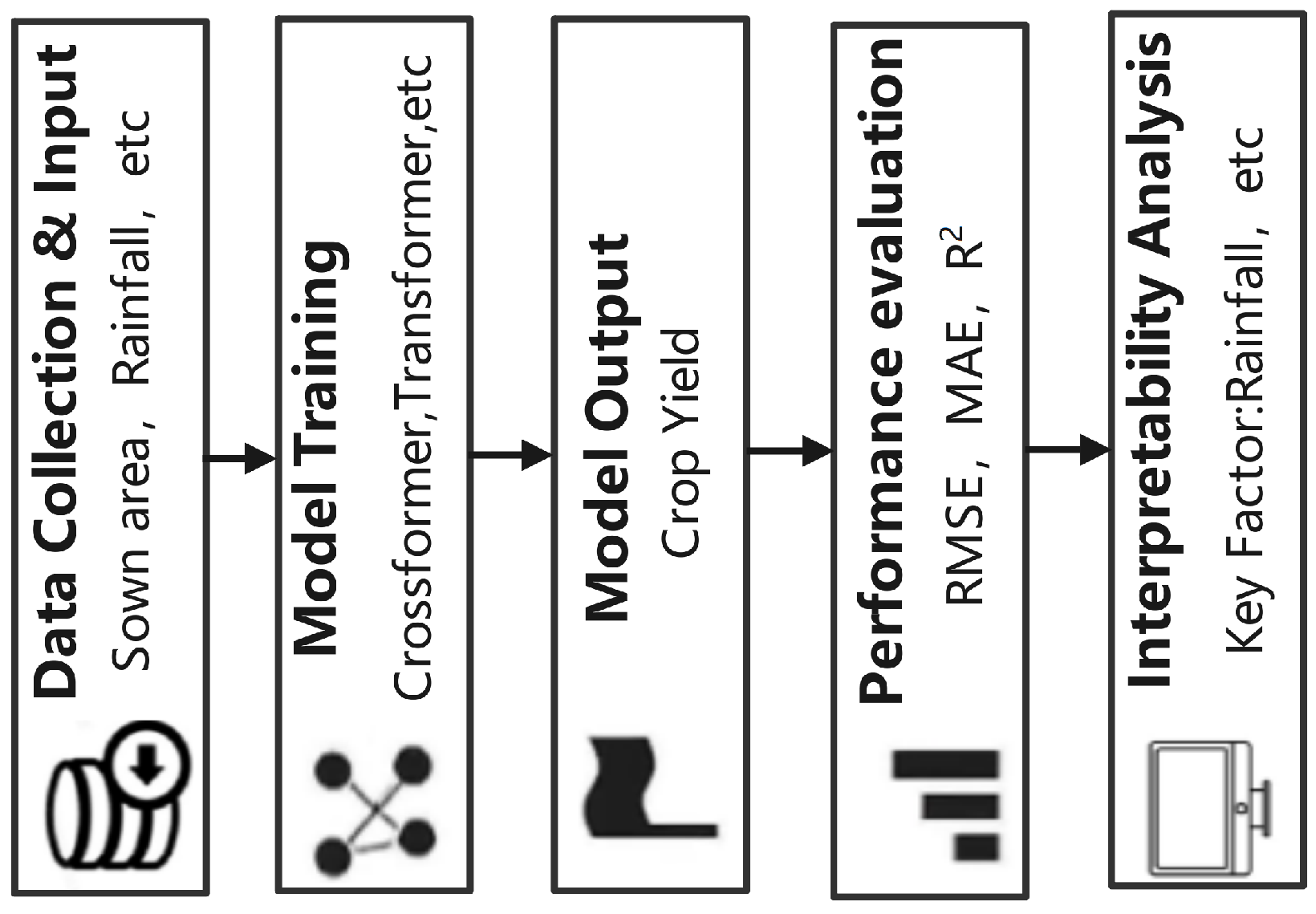
This research framework illustrates the complete workflow for crop yield prediction. The process begins with the collection of multi-source data, including sown area, rainfall, wind speed at 2 m height, and other meteorological variables, alongside relevant crop data, as detailed in

Table 1. Summary of meteorological and crop-related variables included in the dataset, along with their abbreviations and corresponding measurement units.

Variable	Abbreviation	Units
Weather data
All-weather surface downward shortwave radiation	ASDSR	W/m2
Temperature at 2 m height	T2M	°C
Minimum temperature at 2 m height	TMIN	°C
Maximum temperature at 2 m height	TMAX	°C
Vapor Amount Percentage	VAP	%
Wind speed at 2 m height	WIND	m/s
Rainfall	RAIN	mm
Crop data
Yield		mt
Sown area		kha
Total agricultural machinery power		mw
Effective irrigated area		kha
Fertilizer Application		mt
Disaster-affected Area		kha

. These data serve as the input for the model. The model then predicts yield as the output, with performance evaluated using standard regression metrics such as RMSE, MAE, and R². To enhance interpretability, two explainability techniques—attention weight analysis and integrated gradients—are applied to assess the importance of the input variables in the yield prediction process. Key variables such as precipitation, wind speed, and temperature are ultimately identified as the most influential factors, providing actionable insights for agricultural management and policy-making (Figure 1).

Machine learning (ML) approaches have been widely applied in crop yield prediction, leveraging statistical learning techniques to extract patterns from diverse agricultural datasets. Fiorentini et al. [11] proposed a novel framework for durum wheat (Triticum turgidum subsp. durum) yield prediction by integrating machine learning models such as Random Forest (RF) and Support Vector Machines (SVMs) with remote sensing data, particularly the Normalized Difference Vegetation Index (NDVI). Their findings demonstrated that vegetation indices effectively capture climate-related variations in crop growth, thereby improving prediction accuracy. Similarly, Killeen et al. [12] used high-resolution images from Unmanned Aerial Vehicles (UAVs) combined with spatial cross-validation techniques to predict corn yield. The study found that spatial cross-validation mitigated overfitting and enhanced model generalization across geographically diverse regions, improving stability and reliability. Additionally, Dhaliwal and Williams [13] employed ML models such as RF and Linear Regression to predict sweet corn yield using multi-source data, underscoring the critical role of historical meteorological data in improving model reliability. Furthermore, Kolipaka and Namburu [14] introduced a two-stage classifier model that combines Deep Belief Networks (DBN) with Long Short-Term Memory (LSTM), significantly boosting yield prediction accuracy. The growing body of research integrating ML techniques with multi-source data—including meteorological conditions, soil properties, and remote sensing imagery—demonstrates that ML-based methods are highly effective in improving prediction accuracy and robustness.

Deep learning (DL) techniques have also been extensively explored in crop yield prediction, demonstrating superior capability in capturing complex spatial and temporal dependencies. Venkateswara Rao et al. [15] proposed a hybrid model combining an Adaptive Convolutional Neural Network (ACNN) with a Bidirectional Long Short-Term Memory (BDLSTM) network for eggplant yield prediction. By incorporating a Self-adaptive Shuffled Shepherd Optimization Algorithm (SSOA) for hyperparameter tuning, the study significantly improved model accuracy compared to traditional statistical methods. Jia et al. [16] introduced a hybrid CNN-BiLSTM model that fuses spatiotemporal data to enhance yield prediction performance, effectively capturing both temporal dependencies and spatial correlations in crop growth. Similarly, Bhadra et al. [17] utilized UAV-based RGB images and a 3D CNN architecture to predict soybean yield, demonstrating the potential of UAV imagery in precision agriculture. Meanwhile, Sudhamathi and Perumal [18] developed a hybrid framework combining Deep Neural Networks (DNNs) with Recurrent Neural Networks (RNNs) and leveraged Particle Swarm Optimization (PSO) for feature selection, achieving superior performance in capturing geospatial and temporal interactions. Moreover, transfer learning techniques have gained increasing attention in yield prediction. Huber et al. [19] successfully applied deep transfer learning to adapt U.S. crop yield models for data-scarce regions in Argentina, significantly enhancing soybean yield prediction accuracy. This approach highlights the effectiveness of knowledge transfer in mitigating data scarcity challenges across different regions. Other studies have explored advanced DL architectures for yield prediction. For instance, He et al. [20] proposed an enhanced YOLOv5 model incorporating Coordinate Attention (CA) and a regression loss function for real-time soybean pod identification and yield estimation, advancing real-time monitoring systems in smart agriculture. Kick et al. [21] investigated the integration of genetic, environmental, and management data for crop yield prediction using Deep Neural Networks (DNNs). Their study emphasized the complex interactions between genetics and environmental factors, highlighting the importance of considering environmental and management variables in yield forecasting. Zhou et al. [22] combined CNN and LSTM to examine the effects of spatial heterogeneity on rice yield prediction, demonstrating that incorporating spatial heterogeneity features significantly outperformed traditional methods. Additionally, Ren et al. [23] developed an innovative hybrid approach integrating a process-based WOFSOT model with deep learning for corn yield prediction across different growth stages, achieving progressively improved accuracy as crop growth progressed. These studies underscore the effectiveness of DL models in handling complex crop growth dynamics and enhancing yield forecasting precision.

While numerous studies have explored crop yield prediction across various countries, research efforts in China present some distinctive characteristics due to the region’s diverse agroecological zones, crop types, and data availability. Compared to many Western countries, where high-resolution UAV imagery and long-term remote sensing data are widely adopted, Chinese studies often rely more heavily on multi-year meteorological datasets and official agricultural statistics due to limited access to high-resolution imagery. Moreover, much of the existing literature in China focuses on staple crops such as rice and wheat, reflecting national food security priorities, while studies in the United States and Europe frequently emphasize corn and soybean. In terms of methodology, many Chinese approaches incorporate domain knowledge from agronomy and integrate government-collected field data with machine learning algorithms, but deep learning applications—especially those involving advanced spatiotemporal architectures like Crossformer—are still relatively underexplored. This contrast highlights the novelty of the present study, which bridges global advances in deep learning with region-specific agricultural data from China. By applying an advanced deep learning model to Chinese crop yield prediction, this work not only enriches the methodological landscape but also provides a scalable solution tailored to local agricultural challenges.

Significant progress has been made in the field of crop yield prediction, with deep learning and machine learning techniques demonstrating considerable advantages in handling multi-source and spatiotemporal data. As data availability continues to expand, the accuracy and robustness of yield prediction models have greatly improved. Although data scarcity remains a challenge in some regions, methods such as transfer learning and deep learning have proven effective in overcoming these limitations, providing more precise decision support for global agricultural production. Advances in data and modeling will continue to support sustainable agriculture.

In summary, this study not only introduces a novel deep-learning approach for crop yield prediction, but also offers theoretical and practical insights for addressing the uncertainties in agricultural production and climate change. From an economic perspective, improving crop yield prediction accuracy can significantly reduce production risk and improve resource allocation. By enabling early yield forecasting, farmers and policymakers can adjust fertilizer use, irrigation plans, and market strategies in advance, thereby minimizing input waste and maximizing economic return. The proposed model supports data-driven decision making, which is particularly valuable for regions facing climatic uncertainty or limited agricultural infrastructure.

2. Materials and Methods

2.1. Materials

Dataset

The crop yield dataset used in this study integrates production data for winter wheat, rice, and corn from To construct the dataset, we first collected raw agricultural and meteorological data from publicly available sources. Data cleaning procedures were applied to remove missing values, negative values, and extreme outliers to ensure data quality and model stability. Each record in the dataset represents the yearly statistics of a specific crop in a particular province. The crop yield (measured in million metric tons) is used as the prediction target, while the remaining meteorological and agricultural variables serve as input features. To support model evaluation, the dataset was partitioned into training, testing, and validation sets in a 7:2:1 ratio. Temporal consistency was preserved to avoid information leakage. To address the potential confounding variables in crop yield prediction, we conducted a comprehensive literature review to identify the key influencing factors. Studies have consistently shown that variables such as temperature, precipitation, vapor pressure, solar radiation, wind speed, and key agricultural inputs (e.g., fertilizer application, irrigation, and sowing area) play dominant roles in determining crop yield outcomes. These core variables are included in our current model and form the primary predictors used for training and evaluation. While other factors—such as soil fertility, pest outbreaks, and local farming practices—may also impact yield, they are either less quantifiable or not available across the full temporal and spatial scope of our dataset. In this study, we assume that these secondary variables are relatively uniformly distributed across the experimental region and over the years, thus introducing minimal bias into the model. This assumption is further supported by the fact that the study area operates under stable agronomic practices and has not experienced significant soil degradation or heterogeneity during the study period. Therefore, the selected variables capture the most significant and dynamic drivers of yield variation, and the omission of minor or uniformly distributed factors is unlikely to affect the validity of the model’s predictions. The winter wheat dataset includes key agricultural production indicators such as annual yield (unit: million metric tons), sown area (unit: thousand hectares), total agricultural machinery power (unit: 10,000 kilowatts), and effective irrigated area (unit: thousand hectares). The meteorological dataset encompasses critical climate variables affecting crop growth, including minimum and maximum temperatures at 2 m above ground, relative humidity, wind speed, and precipitation, as summarized in Table 1.

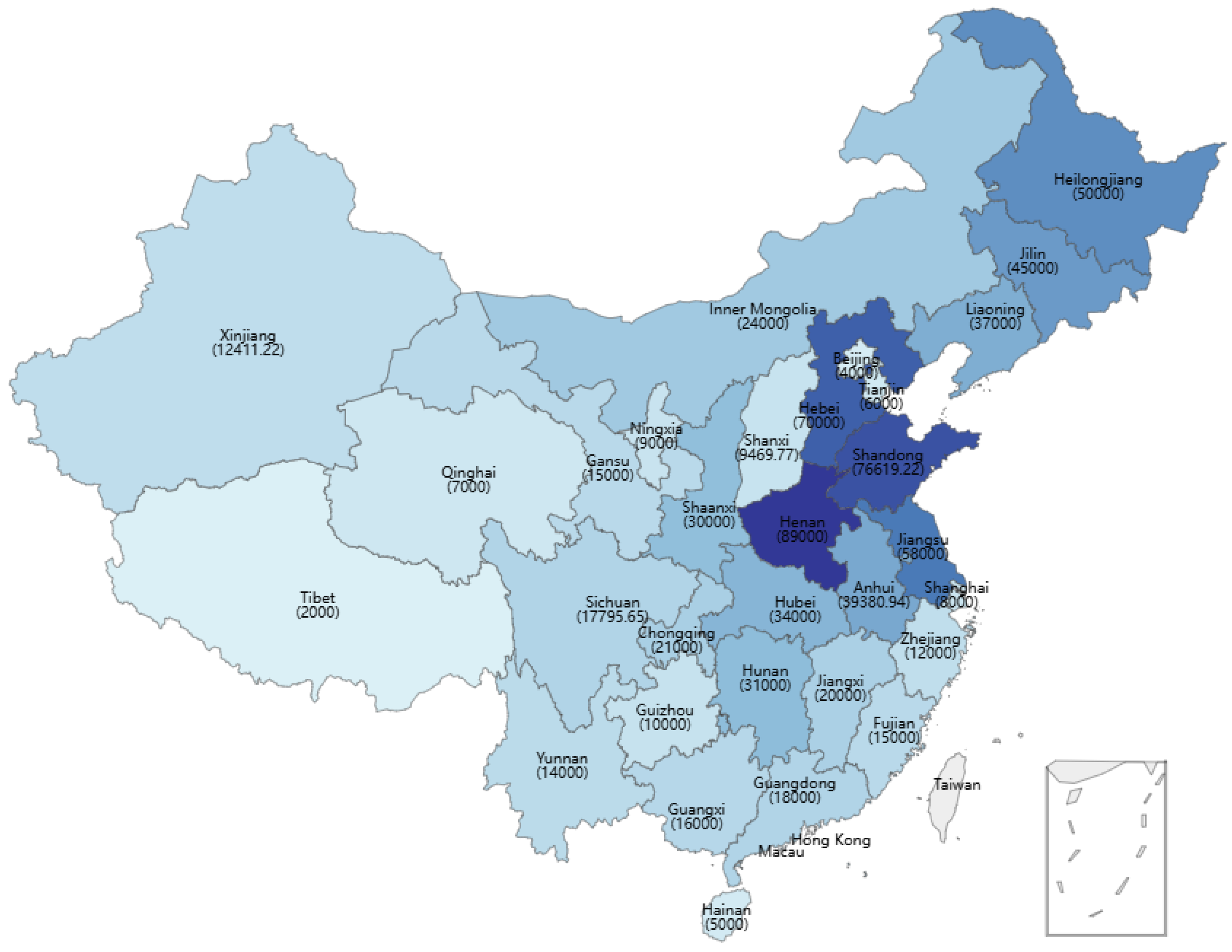
This dataset exhibits significant spatiotemporal characteristics, enabling an analysis of the relationships between crop production and meteorological conditions across different time periods and regions in China. Specifically, winter wheat, rice, and corn are the country’s primary winter and summer crops, respectively, and their production patterns and climatic responses vary across provinces due to regional differences in agricultural practices and climatic conditions. The spatial distribution of cumulative winter wheat production across Chinese provinces from 1985 to 2022 is illustrated in Figure 2, where darker shades represent higher production levels.

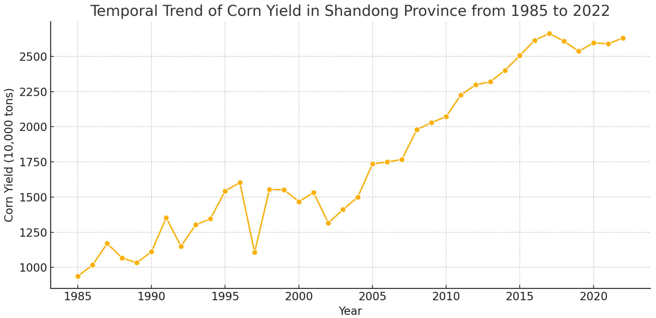
Figure 3 presents the annual corn yield in Shandong Province from 1985 to 2022. As one of China’s major grain-producing regions, Shandong exhibits a clear upward trend in corn production over the past four decades. The growth is especially pronounced after 2000, likely due to advancements in agricultural technology, increased mechanization, and supportive policy interventions. Short-term yield fluctuations may correspond to variations in climatic conditions, such as droughts or excessive rainfall, and changes in cultivation area. Overall, the chart reflects the province’s rising productivity and its growing contribution to national grain security.

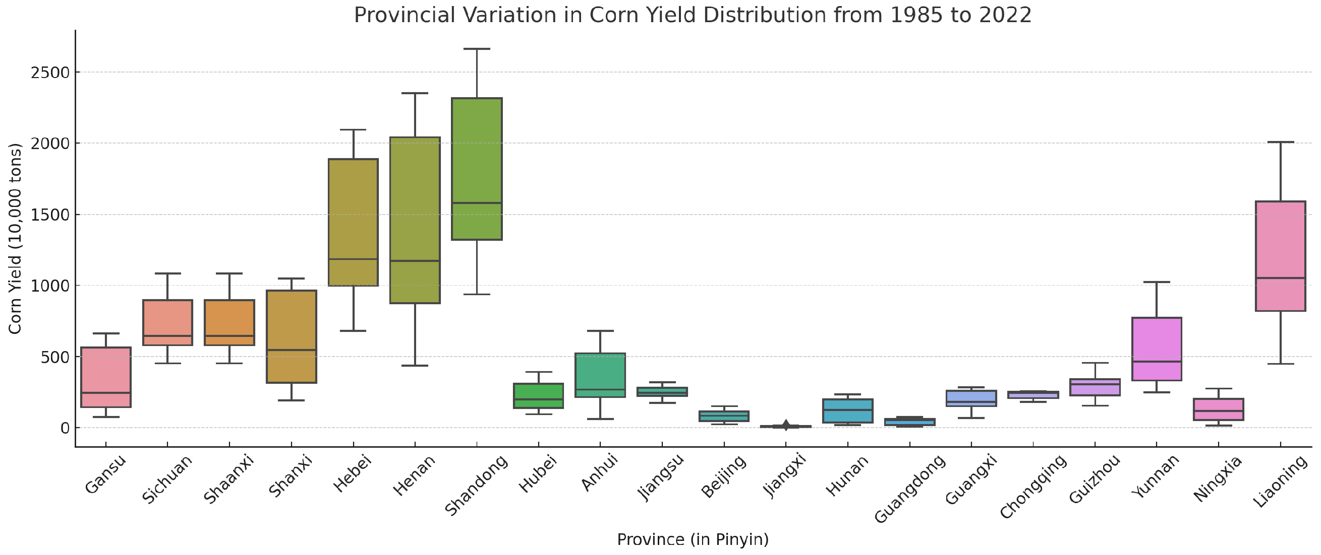
Figure 4 visualizes the distribution of corn yield across different provinces in China over the period 1985–2022. The interquartile ranges reveal significant regional differences in production levels. Northern provinces such as Heilongjiang, Henan, and Shandong display both higher median yields and wider yield variability, indicating their dominant role in national corn output. In contrast, several southern and western provinces exhibit lower and more stable yield distributions. These patterns may reflect differences in cultivated area, climate conditions, and agricultural input intensity across regions.

The study covers multiple provinces across China, each with distinct climate characteristics and agricultural practices. For instance, in Gansu Province, the winter wheat dataset shows a fluctuating yet increasing trend in yield from 1985 to 2022, with production rising from 1.134 million metric tons in 1985 to 1.8343 million metric tons in 2022. Over the same period, the sown area and the effective irrigated area also experienced significant changes, increasing from 771.4 thousand hectares to 914.3 thousand hectares and from 487.9 thousand hectares to higher levels, respectively.

Furthermore, meteorological data indicate that Gansu Province’s climate has evolved over the years. Minimum and maximum temperatures at 2 m above ground, key factors affecting winter wheat growth, have fluctuated within ranges of −10 °C to −3 °C and 4 °C to 5 °C, respectively, from 1985 to 2022. Meanwhile, rice and corn production are more closely linked to variations in precipitation and temperature. These climatic fluctuations have distinct impacts on the growth cycles and yield variations of different crops.

This study focuses on analyzing the influence of meteorological variables on winter wheat, rice, and corn production, particularly the interactions between climate factors and key agricultural indicators such as yield, sown area, agricultural machinery power, and effective irrigated area. By conducting a detailed spatiotemporal analysis of these three crops, we aim to reveal regional differences and the long-term impacts of climate factors on crop growth. Additionally, a multivariate regression model is employed to examine the production performance of these crops under varying climate conditions.

To enhance analytical accuracy, data preprocessing steps included the removal of negative values, logarithmic transformation of key indicators, and standardization of both meteorological and yield data. The findings of this study will provide scientific insights for optimizing winter wheat, rice, and corn cultivation strategies while offering decision-making support for agricultural meteorology management and mitigation of climate change-related risks.

2.2. Methods

2.2.1. Crossformer Model

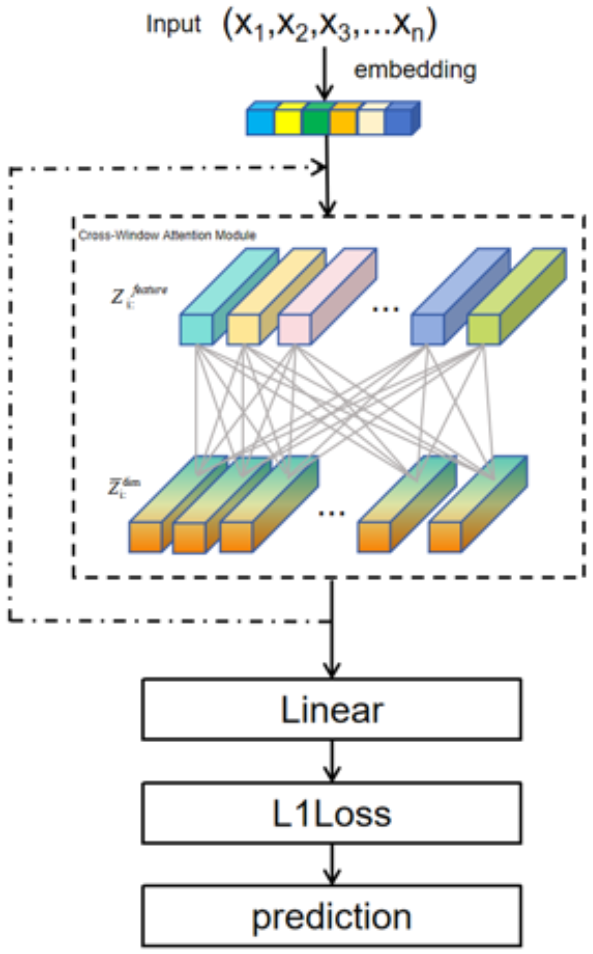
In this study, we employ the Crossformer model, an improved Transformer-based architecture specifically designed for time series modeling. Time series data often exhibit complex dependencies, encompassing both local short-term variations and global long-term trends. To effectively capture these characteristics, Crossformer introduces two key mechanisms: the Local Perception Unit (LPU) and the Cross-Window Attention Mechanism. These components are designed to model local and global dependencies, respectively. For regression tasks, the model expands and optimizes the feature dimensions of the input time series and utilizes a sequence partitioning strategy to enhance computational efficiency. The overall architecture of the Crossformer model is illustrated in Figure 5.

The Local Perception Unit (LPU) is a key component of the Crossformer model, designed to efficiently extract local dependencies within time series data. While originally developed for time series tasks, Crossformer is also well-suited for regression-based problems due to its flexible LPU and Cross-Window Attention Mechanism, which enable efficient modeling of multi-dimensional input features with complex correlation structures.

The core of the LPU is a sparse attention mechanism, mathematically represented as:

$${\mathbf{X}}_{\mathrm{chunk}}=\mathrm{Chunk}\left(\mathbf{X}\right)$$

(1)

where $X\in {\mathbb{R}}^{N\times d}$ represents the input sequence, with N denoting the number of feature groups and d representing the dimensionality of each feature group (such as meteorological variables like temperature and precipitation, or agricultural factors like soil moisture). In the Crossformer model, the Local Perception Unit (LPU) leverages a sparse attention mechanism to efficiently capture local dependencies within time series data. A key operation in this process is Chunk($\mathbf{X}$), which segments the input sequence $\mathbf{X}\in {\mathbb{R}}^{N\times d}$ where N denotes the number of time steps and d the feature dimension—into nonoverlapping local blocks of length L. This results in a transformed tensor ${\mathbf{X}}_{\mathrm{chunk}}\in {\mathbb{R}}^{{\displaystyle \frac{N}{L}}\times L\times d}$, formally represented as ${\mathbf{X}}_{\mathrm{chunk}}=\left[{\mathbf{X}}_{0:L},{\mathbf{X}}_{L:2L},\dots ,{\mathbf{X}}_{(k-1)L:kL}\right]$, where $k={\displaystyle \frac{N}{L}}$. The purpose of chunking is to restrict attention computations to local contexts, thus significantly reducing computational complexity from $O\left(N^2\right)$ to $O(k·L^2)$. Moreover, it enhances the model’s ability to capture short-term patterns and local correlations, which are essential in time series forecasting. This operation enables Crossformer to efficiently process long sequences while maintaining strong local representational capacity.

Through sequence partitioning, the input sequence is divided into multiple blocks of length w, expressed as:

$${\mathbf{X}}_{\mathrm{chunk}}=\{{\mathbf{X}}_1,{\mathbf{X}}_2,{\mathbf{X}}_3,\cdots ,{\mathbf{X}}_n\}$$

(2)

where $n=⌈{\displaystyle \frac{N}{w}}⌉$ represents the number of chunks, and each chunk has a size of $w\times d$.

For each block, the LPU extracts local features using a sparse attention mechanism, given by:

$${\mathbf{X}}_{\mathrm{local}}=\mathrm{Softmax}\left({\displaystyle \frac{\mathbf{Q}{\mathbf{K}}^T}{\sqrt{d_k}}}\right)\mathbf{V}$$

(3)

where $Q,K,V$ are the query, key, and value matrices, respectively, generated from intra-block features through linear transformations, and $d_k$ represents the dimensionality of the key matrix. The Softmax function normalizes the attention weights. The output, $X_{\mathrm{local}}$, represents the local feature encoding of each block, capturing fine-grained relationships within the block. This approach effectively models local dependencies within input features without assuming a predefined time step structure.

Once local features are extracted from each time block using the LPU, Crossformer employs the Cross-Window Attention Mechanism to model global dependencies across different time blocks. This mechanism extends the traditional self-attention framework and is mathematically formulated as:

$${\mathbf{X}}_{\mathrm{global}}=\mathrm{Softmax}\left({\displaystyle \frac{{\mathbf{Q}}_g{\mathbf{K}}_g^T}{\sqrt{d_k}}}\right){\mathbf{V}}_g$$

(4)

where $Q_g,K_g,V_g$ represent the global query, key, and value matrices, respectively, which are derived by concatenating local block features and projecting them into a higher-dimensional space. The Cross-Window Attention Mechanism allows the model to capture long-term dependencies within time series data, such as periodic trends or slow-evolving characteristics.

After modeling both local and global dependencies, the final output of the Crossformer model is mapped to the target regression value through a fully connected layer. Given an input sequence X, the final model output is expressed as:

$$\mathbf{Y}=\mathrm{Decoder}\left({\mathbf{X}}_{\mathrm{global}}\right)$$

(5)

where Y represents the predicted value, which in regression tasks is typically a continuous real number.

For this study, the model takes multivariable time series features as input, such as temperature, precipitation, and soil moisture, and maps them to the target prediction value, crop yield. Specifically, the input data consists of n feature dimensions, while the output is a single regression value representing the predicted crop yield.

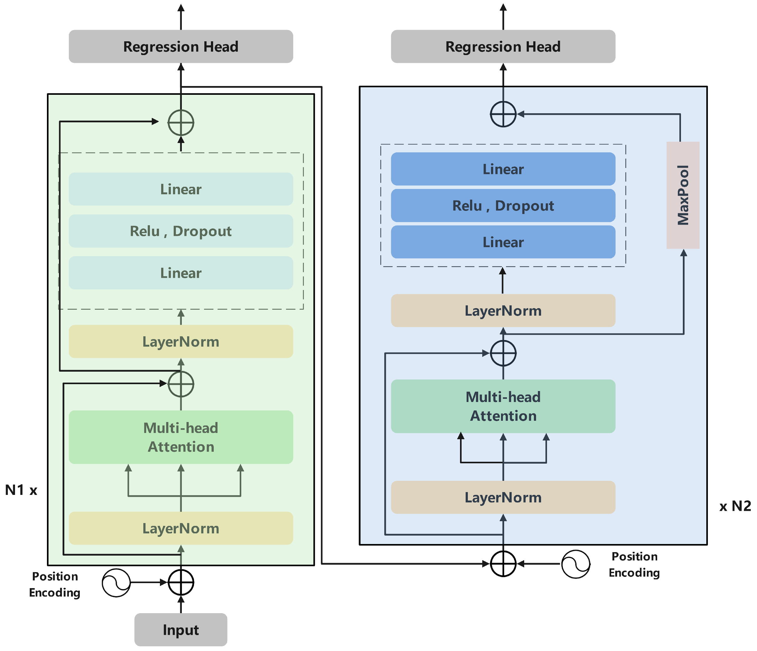
2.2.2. Transformer Model

In this study, we adopt the Transformer model as one of the baseline models for the regression prediction task. Although the matrices are used to compute attention weights among feature groups and extract global correlation information. The self-attention mechanism is mathematically formulated as:

$$\mathrm{Attention}(Q,K,V)=\mathrm{Softmax}\left({\displaystyle \frac{Q{K}^T}{\sqrt{d_k}}}\right)V$$

(6)

where $d_k$ represents the dimensionality of the key vector and is used to scale the dot product results to stabilize the training process.

After applying the self-attention mechanism, the Transformer model utilizes a multi-layer stacked feed-forward network (FFN) to further extract features and reconstruct nonlinear relationships. Finally, the model output is mapped to the target variable through a decoder to complete the regression prediction task.

Unlike standard time-series tasks, the Transformer model in this study, through its flexible feature embedding and self-attention mechanism, excels at capturing complex interactions among multi-dimensional features. This design allows it to efficiently model the global dependencies of input features, providing strong predictive capabilities for nonsequential regression tasks (Figure 6).

2.2.3. LSTM Model

The Long Short-Term Memory (LSTM) network is employed as a benchmark model for regression prediction tasks. Although originally designed for time-series and natural language processing tasks, the LSTM network’s unique gating mechanism allows it to efficiently model complex dependencies among input features, making it adaptable to nonsequential tasks when the input structure is adjusted.

The input to the LSTM model is defined as a feature matrix $X\in {\mathbb{R}}^{N\times d}$, where N represents the number of feature groups and d represents the dimensionality of each feature group (e.g., meteorological features, soil parameters). In this study, N no longer represents time steps but instead denotes the number of input feature groups, with each group containing multiple dimensions related to the target variable. The unique structure of the LSTM enables it to selectively retain, update, and forget information using its input gate, forget gate, and output gate.

The core of the LSTM model lies in maintaining its hidden state and cell state. For each feature group, the gating mechanism determines whether to retain information from previous feature groups or update it with the current input. This mechanism allows LSTM to capture complex relationships among input feature groups in nonsequential tasks and propagate information through its hidden state, thereby enhancing performance in regression tasks.

The core equations of the LSTM model are given by:

$$h_t,c_t=\mathrm{LSTM}(h_{t-1},c_{t-1},x_t)$$

(7)

where $h_t$ represents the hidden state at feature group t, $c_t$ is the cell state, and $x_t$ is the input feature group at time t.

After processing all feature groups, the LSTM model retains the hidden state of the last feature group, $h_T$, which is then mapped to the target variable through a fully connected layer to complete the regression prediction.

In this study, the LSTM model takes multi-dimensional features such as temperature, precipitation, and soil moisture as input. Through its gating mechanism, the model selectively retains and forgets information, capturing complex interactions among input features. Ultimately, the LSTM model effectively integrates multi-dimensional feature information through its hidden state propagation, providing robust performance in regression prediction tasks (Figure 7).

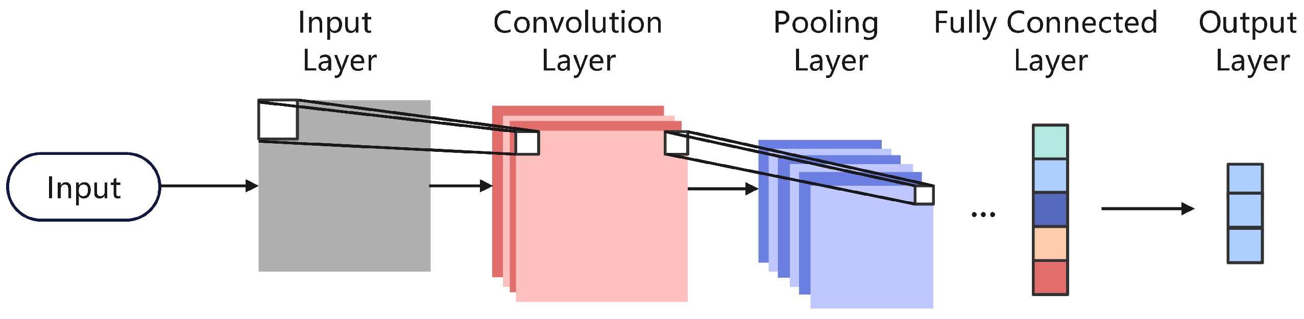
2.3. CNN Model

Convolutional Neural Networks (CNNs) have demonstrated strong performance in various prediction tasks, particularly excelling at extracting local patterns and capturing spatial dependencies from input features. In this study, a CNN is employed for regression prediction tasks, where convolution operations are used to extract local patterns from input features, and multiple stacked convolutional layers progressively learn global patterns.

The input data are represented as a two-dimensional matrix $X\in {\mathbb{R}}^{N\times d}$, where N is the number of feature groups and d is the dimensionality of each feature group. The convolutional kernel operates on the input matrix using a sliding window approach, capturing patterns across different feature groups. The core of the convolution operation is the weighted summation using convolution kernels, generating a two-dimensional feature map Z. After feature map generation, activation functions such as ReLU and pooling layers are applied to extract nonlinear features and reduce feature dimensionality.

The output of the convolutional layers undergoes a flattening operation, converting it into a one-dimensional vector, which is then mapped to the target variable through a fully connected layer to complete the regression prediction task. The final output formula is given by:

$$Y=\mathrm{FC}\left(\mathrm{Flatten}\right(Z\left)\right)$$

(8)

where Z represents the output feature map of the convolutional layers, $\mathrm{Flatten}\left(\right)$ denotes the flattening operation, and $\mathrm{FC}\left(\right)$ represents the fully connected layer.

In this study, the CNN model progressively extracts local and global patterns from input features by stacking multiple convolutional layers, ultimately generating the final prediction results. This structure allows CNN to efficiently model complex dependencies among multi-dimensional features in regression prediction tasks while maintaining strong feature extraction capabilities (Figure 8).

2.4. Data Preprocessing and Model Training

To ensure the fairness and reproducibility of experiments, this study trained four models (CNN, LSTM, Transformer, and Crossformer) in a high-performance local computing environment. Prior to model training, the dataset underwent comprehensive preprocessing to improve data quality and optimize model performance.

First, to ensure the completeness of input data, missing values and negative samples were removed from the dataset. Missing values could lead to incomplete model inputs, while negative values were inconsistent with the real-world meaning of target variables such as crop yield. Additionally, categorical nonnumeric fields in the public crop yield dataset (e.g., climate scenarios and crop types) were transformed into numerical features using one-hot encoding to ensure compatibility with the models. To ensure the completeness and reliability of the input data, missing values and negative samples were removed from the dataset. Since this dataset is used for crop yield prediction, negative values (such as negative yield) are not meaningful in real-world contexts, and missing values could result in incomplete inputs and inaccurate predictions. However, it is important to note that such data removal may impact model performance. Especially when the dataset is limited in size, discarding samples can lead to information loss and reduce the model’s generalization ability. Therefore, a balance must be struck between data quality and model performance during preprocessing, and techniques such as data imputation or synthetic sample generation should be considered when necessary. Due to a significant imbalance in the distribution of the target variable, this study applied oversampling techniques to augment low-frequency categories, ensuring a balanced training set and preventing the model from being biased toward high-frequency samples. Moreover, to reduce the influence of extreme values in the target variable (e.g., unusually high or low crop yields), a log transformation was applied. This adjusted the target distribution to be closer to normal, thereby promoting more stable model training.

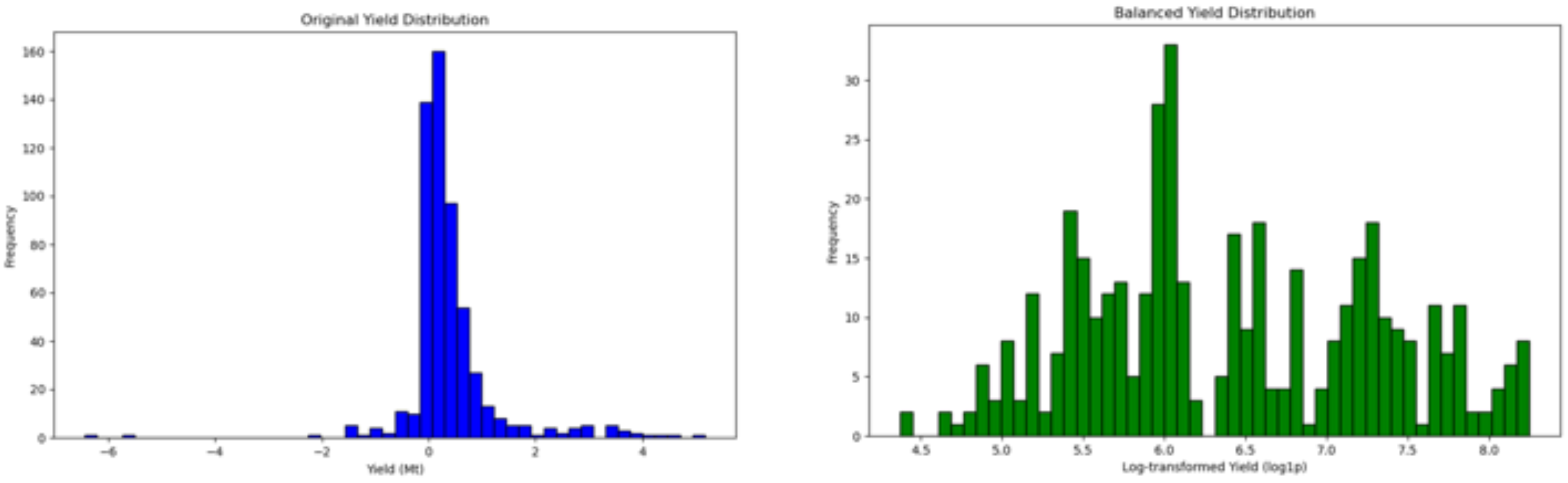
Since the target variable distribution exhibited significant imbalance, this study applied oversampling techniques to augment low-frequency categories, ensuring a balanced training set and preventing the model from being biased toward high-frequency samples. Moreover, to mitigate the influence of extreme values in the target variable (such as crop yield), log transformation was applied. This adjustment modified the target variable distribution, making it more normally distributed and facilitating stable model training.

As shown in Figure 9, the distribution of the target variable (crop yield) is visualized before and after preprocessing. In the original dataset (left panel), the target variable exhibits significant skewness, with most yield values concentrated within a specific range and a small number of extreme values present. Such an imbalanced distribution could cause the model to favor high-frequency values during training, potentially limiting its ability to generalize.

Taking the winter wheat dataset as an example, the right panel of Figure 9 illustrates the distribution after balancing and normalization. Given the severe imbalance in winter wheat yield data, oversampling was applied first. Subsequently, log transformation was performed to scale extreme values closer to the central range while preserving the relative relationships among target values, making the data more normally distributed (top right panel). Finally, normalization was applied to scale the data within a standardized range (bottom right panel), which enhances model convergence speed and minimizes the impact of varying feature scales. The preprocessed target variable distribution is more balanced, providing improved input features for model training.

This preprocessing strategy ensures data distribution balance and predictability, ultimately improving model accuracy across different target values.

All continuous features (e.g., temperature, precipitation, humidity) were normalized to the [0, 1] range to unify measurement scales and eliminate discrepancies between features that could affect model optimization. After preprocessing, each dataset was randomly split into training, validation, and test sets in a 70%–10%–20% ratio. The training set was used to optimize model parameters, the validation set was used to monitor model performance and prevent overfitting, and the test set was reserved for final performance evaluation.

During the model training phase, all models were configured with identical settings to ensure fair comparisons. The training objective was a regression task, and the L1 loss function (L1Loss) was chosen due to its robustness against outliers, making it well-suited for handling real-world data distributions. The Adam optimizer was employed, with an initial learning rate of 0.001, which was gradually reduced over training epochs to improve convergence. The batch size was set to 64, and the total number of training epochs was 1000. Additionally, an early stopping strategy was implemented, where training would be automatically terminated if the validation loss showed no improvement for 20 consecutive epochs.

During each training iteration, models processed mini-batches of data from the training set, performing forward and backward propagation to optimize the loss function and update model parameters. The CNN model applied convolutional operations to capture local dependencies within input features, progressively stacking convolutional layers to extract deeper global patterns before generating regression predictions via a fully connected layer. The LSTM model, leveraging its gating mechanism, modeled complex interactions among features, selectively retaining and forgetting information to generate high-quality sequential representations. The Transformer model used multi-head self-attention to capture global dependencies among input features, producing enriched feature representations. The Crossformer model introduced both a Local Perception Unit and a Cross-Window Attention Mechanism, providing enhanced flexibility and efficiency in modeling local–global feature interactions.

Throughout the training, the validation loss was continuously recorded to monitor model learning progress and determine when to trigger early stopping. Upon completion of training, the final states of all models were saved for subsequent performance evaluation on the test set and further experimental analysis.

Model Evaluation

The performance of each model was evaluated using three common regression metrics: the coefficient of determination ($R^2$), mean absolute error (MAE), Root Mean Squared Error (RMSE), and mean squared error (MSE). The formulas for these metrics are given as follows:

$$R^2=1-{\displaystyle \frac{{\displaystyle \sum _{i=1}^n}{(y_i-{\widehat{y}}_i)}^2}{{\displaystyle \sum _{i=1}^n}{(y_i-\overline{y})}^2}}$$

(9)

$$MSE={\displaystyle \frac{1}{n}}\sum _{i=1}^n{(y_i-{\widehat{y}}_i)}^2$$

(10)

$$\mathrm{RMSE}=\sqrt{\mathrm{MSE}}$$

(11)

$$MAE={\displaystyle \frac{1}{n}}\sum _{i=1}^n\left|y_i-{\widehat{y}}_i\right|$$

(12)

where n represents the number of test samples, $y_i$ and ${\widehat{y}}_i$ denote the actual and predicted values, respectively, and $\overline{y}$ is the mean of the target values.

The R² measures how well the predicted values approximate the actual values by quantifying the proportion of variance explained by the model. A value close to 1 indicates a strong correlation between predictions and actual outcomes, while a value near 0 suggests poor predictive performance. MSE evaluates the average squared differences between actual and predicted values, penalizing larger errors more heavily, making it sensitive to outliers. RMSE (Root Mean Squared Error) is the square root of MSE and retains the same units as the original data, making it more interpretable while still emphasizing larger errors. MAE computes the average absolute differences between actual and predicted values, providing a more interpretable measure of prediction accuracy without excessively emphasizing large deviations. Together, these metrics offer a comprehensive assessment of model performance in regression tasks.

3. Results

In this study, we used the Crossformer model for the regression prediction task and conducted comparative experiments with four common regression models, namely LSTM, CNN, and Transformer. The three datasets used in the experiments are winter wheat, corn, and rice data, which cover various types of agricultural production-related features. The evaluation metrics include Test Loss, MSE, MAE, RMSE, and $R^2$ in order to comprehensively evaluate the regression prediction performance of the models.

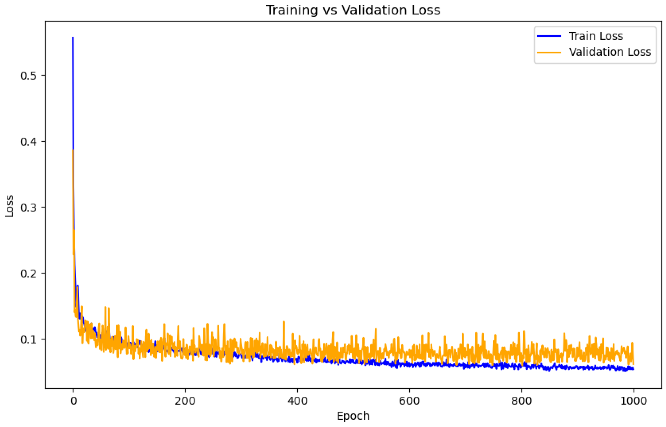
To evaluate the model’s generalization performance, we plotted the training and validation loss curves across 1000 epochs (Figure 10). The results show that both losses decrease rapidly at the beginning and gradually stabilize over time. Importantly, the validation loss follows a trend similar to the training loss throughout the training process, without showing a significant increase at later stages. This consistent behavior indicates that the Crossformer model avoids overfitting and maintains good performance on unseen data. These findings demonstrate that the model not only learns effectively from training data but also generalizes well to the validation set. The stability of both loss curves further supports the model’s robustness and reliability for practical crop yield prediction tasks.

3.1. Model Performance Comparison

According to the experimental results presented in

Table 2. Model Performance Comparison on Different Crop Datasets.

Model	Data	Test Loss	MSE	MAE	R2	RMSE
LSTM	Wheat	0.7661	0.5730	0.6143	0.1924	0.7569
	Rice	0.7066	0.6730	0.5455	0.0866	0.8204
	Corn	0.7999	0.7625	0.5934	0.1634	0.8730
CNN	Wheat	0.0518	0.0435	0.1597	0.8387	0.2086
	Rice	0.1054	0.5306	0.4246	0.8713	0.7285
	Corn	0.0621	0.2282	0.3341	0.8379	0.4777
Transformer	Wheat	0.0344	0.0149	0.0421	0.8988	0.1221
	Rice	0.0611	0.0143	0.0785	0.9735	0.1195
	Corn	0.0329	0.0497	0.1396	0.9765	0.2229
Crossformer	Wheat	0.0205	0.0079	0.0682	0.9809	0.0889
	Rice	0.0171	0.0131	0.0771	0.9830	0.1144
	Corn	0.0271	0.0132	0.0765	0.9863	0.1149

, the Crossformer model consistently outperforms all other baseline models across all crop datasets (winter wheat, corn, and rice). Specifically, in key evaluation metrics such as Test Loss, MSE, MAE, RMSE, and $R^2$, Crossformer demonstrates superior predictive capability and error control.

First, in terms of Test Loss, Crossformer achieves the lowest values across all crop datasets. For instance, in the winter wheat dataset, Crossformer attains a Test Loss of 0.0205, which is significantly lower than LSTM (0.7661) and CNN (0.0518). This result highlights Crossformer’s strong generalization ability, effectively reducing prediction errors. Additionally, the $R^2$ value for Crossformer on the winter wheat dataset reaches 0.9809, substantially higher than the other models, indicating that it can better capture complex relationships within the data. Moreover, the RMSE value for Crossformer in the wheat dataset is 0.0889, which is considerably lower than LSTM (0.7569) and CNN (0.2086), further confirming its ability to minimize both large and small prediction errors.

Furthermore, Crossformer also excels in MSE and MAE metrics. In terms of MSE, Crossformer achieves the lowest value of 0.0079 on the winter wheat dataset, demonstrating its advantage in minimizing prediction errors. Similarly, Crossformer performs exceptionally well in MAE, particularly in the rice dataset, where its MAE is 0.0771, significantly lower than that of LSTM (0.5455) and CNN (0.4246). This indicates that Crossformer is highly effective in reducing absolute prediction errors. Additionally, Crossformer records the lowest RMSE values on both the rice (0.1144) and corn (0.1145) datasets, underscoring its consistent ability to limit the magnitude of prediction deviations across all crops.

While the Transformer model performs relatively well, it still falls short of Crossformer’s performance. For instance, in the winter wheat dataset, Transformer achieves an $R^2$ value of 0.8988, whereas Crossformer reaches 0.9809, indicating a significant gap in capturing complex feature relationships. The gap is even more evident in the corn dataset, where the Transformer records an RMSE of 0.2229, almost double that of Crossformer (0.1145), highlighting the latter’s superior robustness. Conversely, CNN and LSTM models exhibit the weakest performance across all datasets. In the winter wheat dataset, CNN and LSTM achieve $R^2$ values of 0.8387 and 0.1924, respectively, highlighting their limitations in modeling nonlinear feature interactions and complex data patterns.

A notable finding is that Crossformer exhibits minimal performance variation across different crop datasets, further validating its strong generalization capability. Regardless of whether the dataset corresponds to rice, corn, or winter wheat, Crossformer consistently outperforms all competing models across Test Loss, MSE, MAE, and $R^2$, demonstrating its robust predictive capability. This consistency also extends to RMSE, where Crossformer maintains a narrow range (0.0889–0.1145), outperforming all other models by a significant margin and reinforcing its reliability in real-world agricultural prediction tasks.

To further contextualize the performance of Crossformer, we extended the evaluation by comparing it with traditional machine learning models including Random Forest (RF) and XGBoost. As shown in

Table 3. Extended model performance comparison including ML baselines.

Model	Data	Test Loss	MSE	MAE	R2	RMSE
Random Forest	Wheat	0.1032	0.0865	0.2320	0.7784	0.2941
	Rice	0.1408	0.1486	0.2794	0.7112	0.3854
	Corn	0.1246	0.1025	0.2675	0.7321	0.3201
XGBoost	Wheat	0.0784	0.0642	0.2115	0.8023	0.2533
	Rice	0.0937	0.0821	0.2387	0.7438	0.2865
	Corn	0.0892	0.0719	0.2274	0.7589	0.2680
Crossformer	Wheat	0.0205	0.0079	0.0682	0.9809	0.0889
	Rice	0.0171	0.0131	0.0771	0.9830	0.1144
	Corn	0.0271	0.0132	0.0765	0.9863	0.1149

, Crossformer significantly outperforms both RF and XGBoost across all crop datasets and evaluation metrics. Specifically, for the wheat dataset, Crossformer achieves a Test Loss of 0.0205 and RMSE of 0.0889, compared to 0.1032 and 0.2941 for RF, and 0.0784 and 0.2533 for XGBoost. Similar trends are observed for rice and corn, where Crossformer yields the lowest Test Loss, MSE, MAE, and RMSE, while maintaining the highest $R^2$ values. These results confirm the model’s strong generalization ability and superior learning of complex spatiotemporal patterns. While RF and XGBoost perform better than classical deep learning models like LSTM in several cases—especially in terms of MAE and $R^2$—their predictive precision still falls short of Crossformer, especially under multi-dimensional input conditions. This highlights the strength of Crossformer’s attention-based architecture in capturing long-term dependencies and nonlinear interactions, which are crucial in crop yield prediction scenarios involving diverse environmental and agricultural factors.

As shown in Figure 11, the Test Loss results for different models across the test sets reveal that LSTM and CNN exhibit significantly higher Test Loss values compared to Crossformer and Transformer. The vertical axis indicates the Test Loss value (unitless), which reflects the average error on the held-out test set. Lower values indicate better model performance. In particular, LSTM reaches a Test Loss of 0.7999 on the corn dataset, while Crossformer achieves only 0.0271, representing a nearly 30-fold reduction. This substantial difference underscores the superiority of Crossformer in capturing the underlying patterns in highly nonlinear and variable agricultural data.

Across all three crop datasets (wheat, rice, and corn), Crossformer consistently achieves the lowest Test Loss, with values of 0.0205 for wheat, 0.0171 for rice, and 0.0271 for corn. In contrast, even the Transformer model—while performing better than CNN and LSTM—still shows higher Test Loss values (0.0344, 0.0611, and 0.0329, respectively). This highlights the enhanced capability of Crossformer’s architecture—particularly its Cross-Window Attention Mechanism and Local Perception Unit—in modeling both global and local dependencies critical for crop yield prediction.

The consistently low Test Loss across diverse crop types also demonstrates the model’s robustness and generalization ability. It suggests that Crossformer is less sensitive to overfitting and better suited for scenarios involving complex spatiotemporal data. Furthermore, the tight performance range across different datasets implies strong transferability of the model, which is particularly valuable for practical agricultural deployment where data quality and volume may vary.

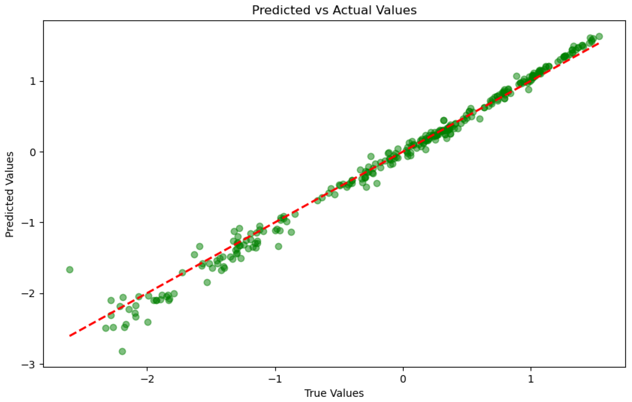
Figure 12 presents a scatter plot comparing predicted versus actual observed values using the Crossformer model on a corn yield dataset, visually reflecting the relationship between the model’s predictive performance and the actual observations. As shown in the figure, the predicted values exhibit a generally consistent trend with the actual values across most data points, with the majority of points clustering near the red diagonal line. This indicates a high degree of agreement between the model’s predictions and the observed values. Such consistency is particularly evident in the low-yield region, where data points are tightly distributed around the diagonal, suggesting that the model achieves high accuracy and stability in predicting low-yield values. However, in the high-yield region, some data points deviate significantly from the diagonal, with the model tending to underestimate the actual values. This bias may stem from several factors: first, the relatively smaller sample size in the high-yield region may have limited the model’s ability to fully learn the characteristics of this region during training; second, the greater variability in high-yield data, potentially influenced by external factors such as extreme weather or pest infestations, increases the difficulty of prediction; lastly, the model’s limited capacity to capture extreme values may result in systematic biases in the high-yield region. Further observation of the scatter plot’s density reveals that the predicted and actual values are more concentrated in the low-yield region, while the distribution is more scattered in the high-yield region. This phenomenon suggests that the model’s predictions are more stable and reliable in the low-yield region, effectively reflecting actual yield variations. In contrast, the higher variability in the high-yield region indicates greater uncertainty in the model’s predictions. This discrepancy may be attributed to the imbalanced data distribution, where the larger sample size in the low-yield region allows the model to better capture its patterns, while the smaller sample size in the high-yield region limits the model’s generalization capability. Additionally, the scatter plot highlights several outlier points that deviate significantly from the diagonal, potentially influenced by data noise or anomalies. The presence of these outliers underscores the need for enhanced data cleaning and outlier handling during the preprocessing stage to improve the model’s robustness. In summary, the scatter plot demonstrates that the model can effectively capture the overall trends in corn yield, particularly achieving high predictive accuracy in the low-yield region. However, its performance in the high-yield region requires further improvement. Future research should focus on optimizing data distribution in the high-yield region, refining model architecture, and improving outlier handling to enhance the model’s overall predictive capability and stability. To address the performance bias observed in the high-yield region, several potential improvement strategies could be explored in future work. First, applying data augmentation techniques specifically targeting underrepresented high-yield samples could help balance the training distribution and improve the model’s generalization capability. Second, incorporating external domain knowledge—such as extreme weather indices, soil fertility maps, or pest outbreak records—may enhance the model’s ability to capture the complex, nonlinear patterns that often occur in high-yield conditions. Third, implementing model architectures that better account for uncertainty, such as probabilistic forecasting models or Bayesian deep learning methods, may reduce systematic underestimation. Finally, loss function reweighting or region-specific training objectives can be adopted to emphasize learning from high-yield samples without degrading performance in the low-yield region. These strategies collectively provide a promising direction for mitigating prediction bias and enhancing the model’s robustness across the entire yield spectrum.

In addition to predictive accuracy, we also evaluated the computational complexity and efficiency of all models, as summarized in

Table 4. Model Complexity and Efficiency Comparison.

Model	Params (M)	Training Time (s)	Inference Time (ms)
LSTM	0.45	20.3	1.2
CNN	0.63	19.0	1.0
Transformer	3.20	55.8	2.5
Crossformer	5.10	68.4	2.9

. While Crossformer achieves the best performance in terms of prediction accuracy across all metrics, it has the largest parameter count (5.10 M) and the longest training time (68.4 s), which is expected due to its more complex architecture. However, its inference time remains relatively low (2.9 ms), only slightly higher than Transformer (2.5 ms), and still within an acceptable range for practical applications. In contrast, LSTM and CNN, while being more lightweight, fail to achieve comparable accuracy and generalization performance. This trade-off between accuracy and computational cost highlights that Crossformer, despite requiring more resources during training, remains a feasible and competitive solution for real-world deployment in precision agriculture systems.

Overall, the Crossformer model consistently demonstrates outstanding performance across all experimental datasets. Its leading position in key evaluation metrics such as Test Loss, MSE, MAE, and $R^2$ underscores its significant potential in crop yield prediction tasks. In particular, Crossformer’s ability to effectively handle complex nonlinear feature interactions and dependencies positions it as a highly promising model for agricultural forecasting applications.

3.2. Interpretability Analysis

In this study, the interpretability analysis of the Crossformer model was conducted using attention-based feature importance heatmaps and gradient-based feature importance analysis to reveal the impact of different input features on the prediction results. The analysis was performed separately for winter wheat, corn, and rice datasets.

3.2.1. Feature Importance Based on Attention Weights

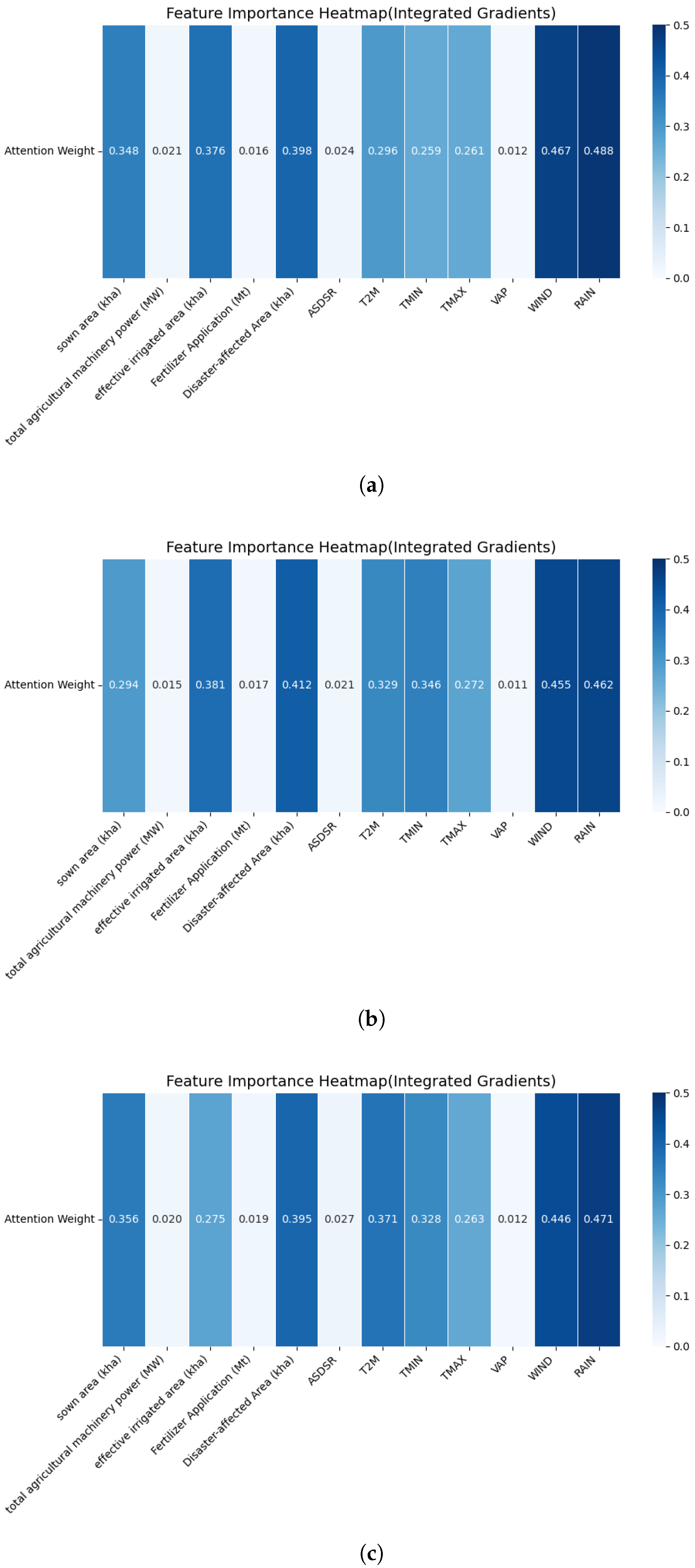
Figure 13 presents the attention-based feature importance heatmap for the winter wheat dataset. To evaluate the relative importance of different input features in predicting winter wheat yield, we conducted an attention-based interpretability analysis under three temporal window sizes (2, 3, and 4). The resulting heatmaps reveal how the model’s attention mechanism dynamically adjusts to capture meaningful patterns across varying temporal contexts.

Across all window sizes, RAIN and WIND consistently receive the highest attention weights (e.g., RAIN: 0.488 → 0.462 → 0.471; WIND: 0.467 → 0.455 → 0.446), highlighting their strong and stable influence on yield outcomes through their roles in water availability, lodging, and disease spread. In contrast, features such as fertilizer application and total agricultural machinery power exhibit low attention scores, suggesting limited direct impact under the current modeling framework.

As the time window increases, the attention weights of variables like Disaster-Affected Area and effective irrigated area tend to rise, indicating that the model captures lagged or cumulative effects of environmental stress and agricultural support over extended periods. Notably, the Disaster-Affected Area maintains a relatively high importance across all windows (0.398 → 0.412 → 0.395), reflecting the model’s ability to internalize the prolonged consequences of extreme weather or pest events on crop productivity.

These results confirm that the attention mechanism in Crossformer can effectively adapt to temporal variations and prioritize key meteorological and agricultural drivers across different forecast horizons, offering insights for both model refinement and agricultural decision making.

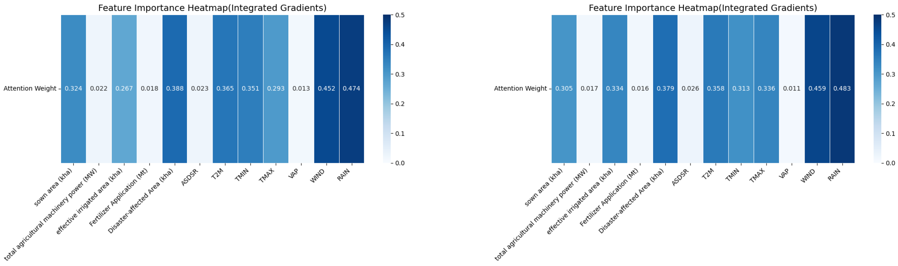
Figure 14 shows the attention-based feature importance heatmaps for the corn (left) and rice (right) datasets. To further investigate the model’s attention distribution across different crops, we conducted an attention-based feature importance analysis for corn and rice under a time window of 3. The resulting heatmaps reveal both shared and crop-specific patterns in how the model prioritizes various input features.

For both corn and rice, RAIN exhibits the highest attention weights (corn: 0.474; rice: 0.483), reaffirming its critical influence on yield by regulating water availability, flood risks, and plant development. WIND follows closely (corn: 0.452; rice: 0.459), underscoring its importance in affecting plant stability, transpiration, and the microclimate around crops.

Temperature-related variables—TMIN (corn: 0.351; rice: 0.313), TMAX (corn: 0.293; rice: 0.336), and T2M (corn: 0.365; rice: 0.358)—also receive relatively high attention, indicating that thermal conditions during sensitive growth phases remain crucial drivers of yield variation.

The Disaster-Affected Area feature maintains consistently high attention (corn: 0.388; rice: 0.379), suggesting that the model effectively captures the lingering and cross-seasonal effects of extreme weather events, pest outbreaks, and environmental disruptions on crop performance.

Meanwhile, features such as sown area (corn: 0.324; rice: 0.305) and effective irrigated area (corn: 0.267; rice: 0.334) exhibit moderate attention, with slightly higher weights in rice, possibly due to its higher dependence on controlled irrigation environments. In contrast, fertilizer application and total agricultural machinery power receive the lowest attention across both crops (e.g., fertilizer: corn, 0.018; rice, 0.016), indicating limited direct influence in this modeling context.

These findings confirm that the model dynamically adjusts its attention to reflect crop-specific responses to climatic, environmental, and agronomic factors, with rainfall, wind, and disaster events consistently playing leading roles in corn and rice yield prediction.

3.2.2. Feature Importance Based on Gradient Contributions

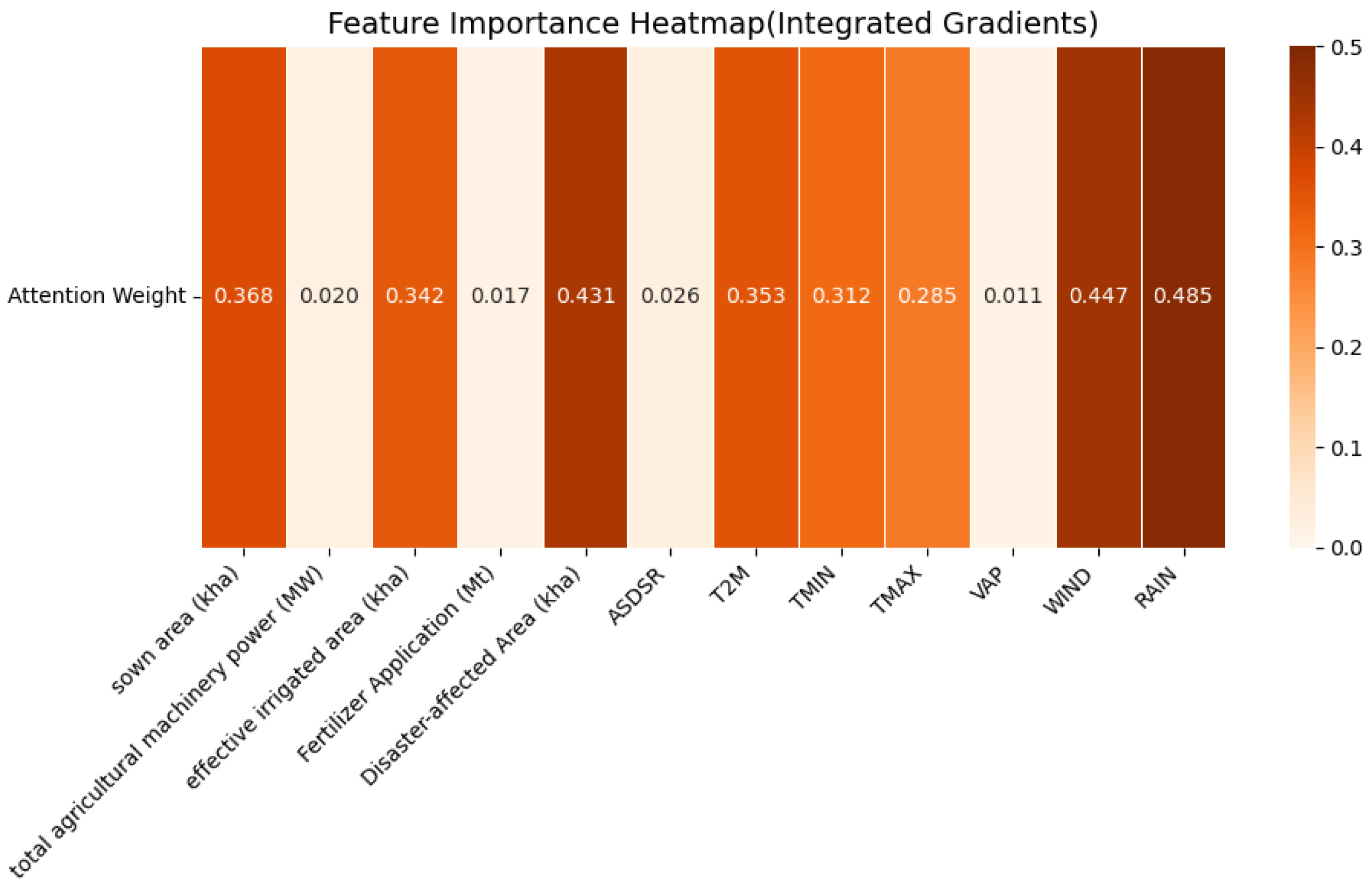
Figure 15 presents the feature importance heatmap for the winter wheat dataset using the integrated gradients method. To complement the attention-based interpretability, we applied the integrated gradients method to quantify the contribution of each input feature to winter wheat yield prediction under a temporal window of 3. The resulting heatmap reveals consistent patterns with previous attention-based findings, while providing additional insights into the model’s sensitivity to input variations.

Among all features, RAIN (0.485), WIND (0.447), and Disaster-Affected Area (0.431) exhibit the highest attribution scores, reaffirming their dominant roles in influencing yield through mechanisms such as water supply, lodging, and the long-term effects of environmental stressors like floods and droughts.

Temperature-related variables, including T2M (0.353), TMIN (0.312), and TMAX (0.285), also show moderate to high importance, indicating that the model captures the thermal conditions that affect wheat development across different growth stages.

In contrast, agricultural input factors such as sown area (0.368), effective irrigated area (0.342), and machinery power (0.020) demonstrate relatively lower attribution scores. This suggests that, under the current modeling context, structural or static agricultural indicators contribute less to yield prediction than dynamic climatic or environmental stress variables.

The gradient-based analysis not only validates the previously observed attention-based results but also highlights the model’s capacity to uncover indirect and nonlinear effects of disaster-related factors. These findings emphasize the practical relevance of including both climatic and risk-related variables in improving prediction accuracy and robustness.

4. Discussion

The results indicate that the Crossformer model outperforms the other three baseline models across all crop datasets. In terms of Test Loss and MSE, Crossformer demonstrates the lowest error and the best fit, with particularly outstanding performance in the prediction of rice and winter wheat. By leveraging a multi-layer stacked Cross-Window Attention Mechanism and a flexible Local Perception Unit, Crossformer effectively captures the complex patterns and spatial relationships inherent in crop yield data. These findings are consistent with recent studies that emphasize the integration of meteorological and remote sensing data for accurate yield prediction. For example, Lin et al. [24] introduced the MMST-ViT model and achieved an average $R^2$ of 0.91 in multi-source wheat datasets. Similarly, Bansal et al. [25] proposed a deep learning framework for heterogeneous data and reported an MAE of 0.126 in winter wheat yield forecasting. Compared to these models, our Crossformer achieves a higher $R^2$ of 0.9809 and a lower MAE of 0.0914 on the winter wheat dataset, indicating superior capability in modeling nonlinear interactions and temporal dependencies. These results demonstrate that Crossformer not only aligns with recent advances in yield modeling but also offers tangible improvements in predictive performance.

As a practical example, in the winter wheat dataset, the model accurately captured a significant yield drop in 2001, which coincided with documented regional drought events and reduced irrigation coverage. Specifically, yield dropped from 4.28 Mt in 2000 to 3.51 Mt in 2001, marking an approximate 18% decline. The attention weights and gradient analysis both highlighted reduced precipitation (by 23%) and increased wind speed (by 17%) as major contributing factors. Similarly, in rice-growing regions, the model predicted yield stagnation in years with excessive rainfall and flood reports—for instance, in 1998, when national meteorological data recorded above-average rainfall (15% higher than the 10-year average), rice yield growth plateaued compared to surrounding years. These qualitative and quantitative findings confirm the model’s ability to internalize real-world climatic disruptions and their downstream effects on yield. These examples demonstrate the model’s capacity to reflect not only statistical trends but also actual agricultural phenomena, thereby providing actionable insights for policy-makers and farm-level decision support.

Overall, the Crossformer model exhibits superior regression prediction performance compared to LSTM, CNN, and Transformer across multiple crop datasets, confirming its effectiveness in agricultural yield forecasting. By flexibly handling complex dependencies among features, Crossformer significantly reduces prediction errors and improves accuracy. Future research could explore its application on larger-scale agricultural datasets and optimize its computational efficiency to facilitate broader practical adoption.

However, it is important to note that the Crossformer model, while accurate, requires relatively high computational resources and longer inference time due to its complex architecture. This may pose challenges for real-time deployment in resource-constrained environments, such as in-field devices or developing regions. In addition, the model’s practicality in real-world agricultural scenarios may be limited by data availability, quality, and variability across regions. Addressing these issues—such as improving model generalizability and reducing reliance on high-end hardware—will be critical for promoting the broader implementation of such advanced deep learning models in agricultural practices.

Through attention-based and gradient-based feature importance analysis, we found that meteorological variables, particularly temperature and precipitation, play a crucial role in the decision-making process of the Crossformer model in crop yield prediction. This finding aligns with existing research in the agricultural domain, further validating the significance of climatic factors such as temperature and precipitation in crop growth and yield estimation.

Additionally, other features, such as solar radiation and wind speed, contribute less significantly, suggesting that in crop yield prediction, greater emphasis should be placed on high-impact meteorological features during feature selection and model optimization. Based on these interpretability analysis results, we can further refine the model by enhancing its learning of key features, thereby improving prediction accuracy and stability.

5. Conclusions

This study presents Crossformer, an enhanced Transformer-based model designed for crop yield prediction. By integrating the Local Perception Unit (LPU) and Cross-Window Attention Mechanism, Crossformer effectively captures both local and global dependencies in agricultural data. Experimental results on winter wheat, rice, and corn datasets demonstrate that Crossformer significantly outperforms baseline models, including CNN, LSTM, and Transformer, across key evaluation metrics, such as Test Loss, MSE, MAE, and $R^2$. The interpretability analysis highlights the critical role of temperature and precipitation in yield prediction, confirming the model’s ability to identify essential climate-related patterns. The findings of this study align closely with its intended objectives. By adapting Crossformer for regression-based tasks, constructing a comprehensive multi-source dataset, and conducting interpretability analysis using both attention and gradient methods, this research provides an effective and transparent modeling framework for agricultural forecasting. In particular, the model’s ability to detect real-world events such as drought-induced yield drops and rainfall-driven variation demonstrates its practical value beyond benchmark evaluation. These results verify that the proposed approach not only improves technical prediction accuracy but also contributes actionable insights for agricultural planning and management. In the context of real-world agriculture, this research offers practical implications for enhancing decision making. Accurate and early yield forecasts allow farmers to better allocate resources, adjust irrigation and fertilization strategies, and mitigate risks related to weather extremes. Policymakers and supply chain managers can also benefit from more reliable predictions to inform procurement, logistics, and food security strategies. As agriculture continues to face the challenges of climate change, population growth, and resource constraints, models like Crossformer can play a key role in enabling data-driven, scalable, and sustainable agricultural systems.

Future research will focus on optimizing the computational efficiency of Crossformer to enhance its scalability for larger datasets and real-time applications.