Abstract
The ripeness of tomatoes is a critical factor influencing both their quality and yield. Currently, the accurate and efficient detection of tomato ripeness in greenhouse environments, along with the implementation of selective harvesting, has become a topic of significant research interest. In response to the current challenges, including the unclear segmentation of tomato ripeness stages, low recognition accuracy, and the limited deployment of mobile applications, this study provided a detailed classification of tomato ripeness stages. Through image processing techniques, the issue of class imbalance was addressed. Based on this, a model named GCSS-YOLO was proposed. Feature extraction was refined by introducing the RepNCSPELAN module, which is a lightweight alternative that reduces model size. A multi-dimensional feature neck network was integrated to enhance feature fusion, and three Semantic Feature Learning modules (SGE) were added before the detection head to minimize environmental interference. Further, Shape_IoU replaced CIoU as the loss function, prioritizing bounding box shape and size for improved detection accuracy. Experiments demonstrated GCSS-YOLO’s superiority, achieving an average mean average precision mAP50 of 85.3% and F1 score of 82.4%, outperforming the SSD, RT-DETR, and YOLO variants and advanced models like YOLO-TGI and SAG-YOLO. For practical deployment, this study deployed a mobile application developed using the NCNN framework on the Android platform. Upon evaluation, the model achieved an RMSE of 0.9045, an MAE of 0.4545, and an R2 value of 0.9426, indicating strong performance.
1. Introduction
Tomatoes are one of the most widely cultivated and consumed vegetable crops, with an exceptionally high global production rate [1]. To meet the continuous demand for daily consumption, tomatoes are currently grown in large quantities within greenhouse environments. Typically, in such controlled settings, tomatoes ripen at an accelerated pace. However, if they become overripe, they are prone to rot, leading to significant economic losses. According to previous studies, losses caused by various diseases and rot account for approximately 30% of the total production [2]. Therefore, it is crucial to accurately classify the growth stages of tomatoes. The rapid and non-destructive identification of tomatoes at different stages of ripeness is necessary for better management of resources during harvesting, transportation, and storage, thus reducing economic as well as labor-related losses [3].
In recent years, traditional image processing algorithms and machine learning techniques have been widely applied across various domains, such as fruit and crop analysis, where they have played a significant role. However, during the course of their application, numerous challenges and issues have also emerged. For instance, excessive reliance on human intervention and vulnerability to complex environmental conditions often result in poor generalization and limited robustness [4]. With the advancement of artificial intelligence, deep learning methods, due to their distinctive capabilities, have demonstrated remarkable efficiency in handling complex scenarios involving occlusion, illumination variation, and scale changes [5,6]. Deep learning-based object detection can be broadly classified into two categories: single-stage detection algorithms and two-stage detection algorithms. The two-stage detection approach consists of an initial stage that generates multiple candidate bounding boxes containing potential objects, followed by a second stage that refines these boxes through localization and classification. Prominent algorithms in this category include Mask R-CNN [7] and Faster R-CNN [8]. As proposed by Wang et al. [9], the MatDet model was introduced for the detection of two categories—green and ripe tomatoes—under complex environmental conditions, achieving a mean average precision (mAP) of 96.14%. Zu et al. [10] designed a Mask R-CNN network for the identification and segmentation of green tomatoes in greenhouse environments, with an F1 score of 92.0%. Furthermore, Minagawa et al. [11] integrated Mask R-CNN with clustering techniques to predict the ripening time of tomato clusters in greenhouses, achieving accuracy (ACC) rates of 80% and 92% in noisy and noise-free environments, respectively. The aforementioned studies validate the high detection accuracy of two-stage detection algorithms. However, these algorithms often overlook critical issues, such as processing time and the inherent complexity of the algorithm itself.
In recent years, single-stage algorithms have gained widespread attention across various research domains, with notable representatives including You Only Look Once (YOLO) and Single-Shot MultiBox Detector (SSD), among which the YOLO series has experienced the most rapid development. The YOLO series algorithms include YOLOv3 [12], YOLOv4 [13], YOLOv5 [14], YOLOv7 [15], YOLOv8 [16], YOLOv9 [17], YOLOv10 [18], and YOLOv11 [19]. While maintaining low complexity and high processing speed, these algorithms also exhibit high detection precision, making them widely applicable across various fields [20]. For instance, Wu et al. [21] designed an efficient object detection network that automatically assigns weights to channel features for apple detection under complex weather conditions, achieving a precision of 90.7%. Zhu et al. [22] proposed an improved network model based on YOLOv8 and applied it within a corn plantation to achieve 128.5 FPS. Additionally, Pual et al. [23] conducted a comprehensive study on peppers using various functionalities within YOLOv8, covering tasks such as recognition, segmentation, classification, and counting, and developed a corresponding Android application, ultimately achieving a detection success rate of 95%. Ren et al. [24] proposed an enhanced YOLOv8 model called YOLO-RCS, which minimizes background interference to capture the distinctive features of “Yuluxiang” pears, achieving an mAP of 88.63% with an inference time of 1.6 ms. Zhu et al. [25] designed a detection model specifically for oil tea fruits in orchards and conducted validation experiments across two datasets, resulting in an mAP of 93.18%, with a model size of only 19.82 MB. These studies demonstrate that single-stage models, while enabling real-time detection, can also maintain high accuracy and are progressively playing a significant role in the field of agricultural recognition and detection.
Recent studies have also explored the detection and classification of tomatoes. Yang et al. [26] classified tomatoes into three categories: mature, immature, and diseased. Their improved model achieved an mAP of 93.7% and a recall of 92.0% on the test set. Gao et al. [27] employed an improved YOLOv5s model for recognizing single-class tomatoes in continuous operational environments, achieving an mAP of 92.08%. Meanwhile, Sun et al. [28] achieved an average detection precision of 92.46% and an ACC of 96.60% on a public dataset, with a frame rate of 74.05 FPS. Chen et al. [29] proposed the MTD-YOLO multi-task cherry tomato network, which enables the detection of both cherry tomatoes and the maturity of fruit clusters. Notably, the model achieved an overall score of 86.6% in its multi-task learning. These diverse approaches to tomato classification provide a valuable foundation for subsequent research in the field. Although these studies are comprehensive, it is evident that there is a lack of detailed research on the finer classification of tomato fruit growth and maturity stages. Tomatoes have a short maturation period and are highly susceptible to various pathogens, often exhibiting multiple concurrent growth states. Therefore, a more rational and effective classification of tomato maturity stages is essential, particularly for accurately identifying tomatoes that are rotten due to disease. Such advancements could facilitate selective harvesting and reduce losses caused by disease-induced decay. Although the aforementioned models have achieved commendable results in detection precision and generalization capabilities, further optimization is still necessary to enhance their adaptability in complex environments. In particular, maintaining high accuracy and robustness while reducing model size will be crucial for enabling broader applications.
With the development of the deep learning embedded field, nowadays, cell phone mobile deployment has become a more popular direction, with remarkable success. The combination of the two empowers key convenient visualization capabilities, which are now widely used for various plant diseases, e.g., lightweight cotton [30] and rice [31]. Similarly, a great deal of research has been conducted on recognizing the plants themselves, such as strawberry [32], winter jujube [33], and so on. Moreover, there is currently a lack of mobile deployment applications for real-time greenhouse tomato recognition. Given the need for the efficient processing of acquired information, quick validation, and timely feedback in mobile applications, the YOLO algorithm, with its high precision, fast efficiency, and ease of lightweight deployment, is particularly well-suited to meet the real-time and practical demands of such end-user applications. Considering these reasons, developing lightweight mobile deployment applications based on the YOLO series could serve as a viable solution for achieving optimal performance on edge devices [34].
Based on the preceding analysis, the key contributions of this study are outlined as follows:
(1) A fine-grained, four-stage classification of tomato maturity (green ripe stage, turning ripe stage, fully ripe stage, and disease-related decay stage) was conducted. Additionally, a data-augmentation-based greenhouse tomato fruit dataset was constructed, encompassing the entire maturation process from the green mature to disease-related decay stages. This dataset also included real-world growth conditions of tomatoes, capturing various angles, lighting intensities, and occlusions.
(2) The GSCC-YOLO improved model was proposed, which effectively reduced computational redundancy and enhanced detection capability while meeting the requirements for real-time detection. Notably, this model demonstrated an mAP50 of 85.3% on a self-constructed dataset, showing a distinct advantage over the current models. To evaluate the model’s generalization ability, validation on public datasets was conducted, achieving an mAP50 of 90.5%.
(3) A mobile application for greenhouse tomato recognition, developed based on the NCNN framework, was successfully deployed on Android devices. Through linear regression experiments and real-world applications, it was demonstrated that the application can accurately and efficiently perform detection in the complex environment of a greenhouse, achieving an R2 value of 0.9426.
2. Materials and Methods
2.1. Dataset Composition
The dataset was primarily divided into three parts. The first part consisted of a self-constructed dataset, which was used for model training and experimentation. The second part comprised a public dataset (https://aistudio.baidu.com/datasetdetail/142431/2, (accessed on 15 December 2024)), which was utilized to validate the generalization ability of the improved model. The third part included the test set from the self-constructed dataset and real-world images captured on-site, which were used for mobile application testing.
2.2. Dataset Construction
2.2.1. Image Collection
The self-built dataset was collected at the tomato cultivation base of Shenyang Agricultural University, located in Shenyang, Liaoning Province, China (123°57′ E, 41°83′ N). The tomato variety cultivated was Dongnong727, with an average plant height of approximately 180 ± 5 cm. Due to the occlusion caused by the upper branches and leaves, it was challenging to capture tomatoes positioned higher up. To address this issue, this study employed a combined approach of using a fixed-point shooting pole and manual photography for image collection. The distance between the shooting pole and the tomato plants was set at 30 cm, with shooting heights of 45 ± 5 cm, 75 ± 5 cm, and 105 ± 5 cm above the ground. Researchers manually photographed tomatoes located outside this height range. The specific shooting positions are illustrated in Figure 1. Image collection covered three time periods: November 2023 to January 2024, July 2024 to September 2024, and December 2024 to January 2025. During each time period, images were collected at the following times: 7:00–9:00 AM, 11:00 AM–1:00 PM, and 4:00–5:00 PM.
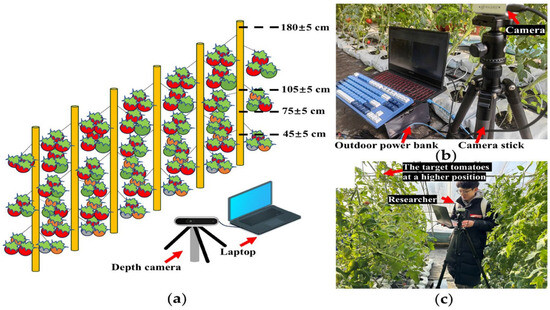
Figure 1.
Dataset image collection diagram. (a) Overview of dataset image collection. (b) On-site image collection at low height, (c) On-site image collection at a higher distance.
To ensure the comprehensiveness and generalizability of the dataset, photographs of tomatoes in various growth stages were captured from multiple angles, as illustrated in Figure 2. A total of 723 images and 9 video clips were recorded, with the videos processed through frame extraction to generate additional images. The process resulted in a total of 763 images, all stored in JPEG format.
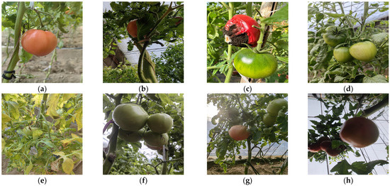
Figure 2.
Images captured from different angles. (a) Front lighting; (b) back lighting; (c) front lighting with mild occlusion; (d) front lighting with moderate occlusion; (e) front lighting with heavy occlusion; (f) back lighting with mild occlusion; (g) back lighting with moderate occlusion; (h) back lighting with heavy occlusion.
2.2.2. Image Annotations and Dataset Composition
Our pre-experimental annotation framework implemented LabelImg to classify the tomato phenological stages into four distinct categories (Figure 3): green ripe stage (T_GreenRP), turning maturity stage (T_BetweenGMP), full maturity stage (T_MaturityP), and disease-related decay stage (T_RotP). The disease-related decay stage includes two types of rot: one caused by delayed harvesting, resulting in natural decay, and the other caused by diseases leading to rotting. The diseases primarily include issues such as wormholes and umbilical rot [35].
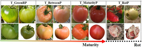
Figure 3.
Illustrative images of tomato fruit at different stages of maturity and decay classification.
2.2.3. Handling of Imbalanced Data Distributions
Due to the rarity of disease-related decay stages in tomatoes under real-world conditions, the imbalance in the dataset may lead to reduced model accuracy and overfitting during training. To address this issue, this study first manually grouped the diseased tomatoes and then applied image processing techniques to mitigate the challenge. The procedure involved the following steps: First, pixel-level segmentation was performed on the images of decayed, disease-affected tomatoes. Second, complex background images without any tomatoes were selected from both videos and photographs. Once these steps were completed, the data synthesis process was carried out. The detailed workflow is illustrated in Figure 4. In total, 21 background images and 7 images of diseased, decayed tomatoes were used. For testing of fits to synthetic data, see Appendix A.
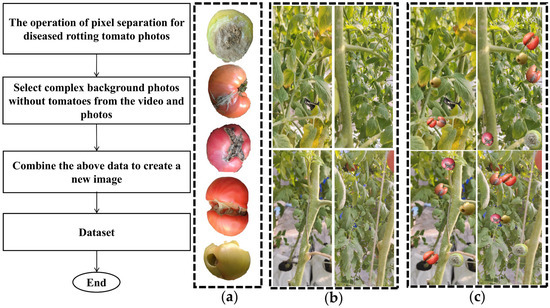
Figure 4.
Dataset synthesis flowchart. (a) Disease-related decay of tomatoes. (b) Complex background without tomatoes. (c) Synthesized image.
2.2.4. Augmentation of the Dataset
We implemented a targeted augmentation pipeline incorporating seven transformation modalities: random translation, Gaussian noise injection, brightness modulation, random crops, rotational variance (±30°), horizontal flipping, and affine shearing. This protocol generated an enhanced dataset containing 6270 annotated samples, systematically partitioned into training ( = 4389), validation ( = 1254), and test subsets ( = 627) following a 7:2:1 stratified allocation. Table 1 quantitatively details the class distribution across maturity stages, including both image counts and their associated annotation instances.

Table 1.
Detailed composition of the tomato growing period dataset.
2.3. GCSS-YOLO
YOLOv8 is a single-stage algorithm designed for tasks such as object detection, instance segmentation, and image classification. Its network architecture is composed of four main components: the input layer, backbone network, neck network, and detection head. YOLOv8 is further categorized into five different network architectures, including YOLOv8n, YOLOv8s, YOLOv8m, YOLOv8l, and YOLOv8x, based on network depth and width thresholds, with each architecture corresponding to variations in the number of sub-modules and kernels [36]. To address a variety of tasks, different architectural approaches were explored. In this study, YOLOv8s was chosen as the baseline model due to its relatively low parameter count, compact model size, and superior precision and detection speed compared to other architectures. The model was then adapted for effective deployment in the recognition of tomato growth and maturation stages on mobile platforms.
However, several challenges arose during practical detection, including complex branch and leaf environments, overlapping and occlusion of multiple targets, and situations where some tomatoes shared similar colors with the branches or leaves. These issues impeded the model’s ability to extract features effectively. In light of these challenges, the YOLOv8s network was specifically improved to ensure both lightweight deployment and efficient, accurate extraction of the growth features of tomatoes at each stage. The modified model was referred to as the GCSS-YOLO model, and its structure is illustrated in Figure 5.
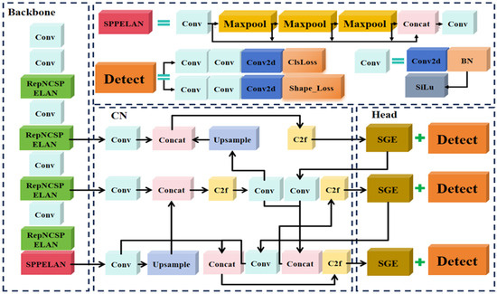
Figure 5.
GCSS-YOLO network architecture diagram.
Specifically, to enhance the backbone network’s ability to focus on the tomato regions in the input images, the lightweight multi-feature decomposition module (RepNCSPELAN) was employed to replace the original C2f structure in the backbone. For the neck network, the PAN structure was retained while the input and output channel dimensions were adjusted to reduce computational redundancy. However, the lightweight modification of the neck network led to an imbalance in the extraction of semantic and spatial features during detection. To address this issue, a Semantic Feature Learning module (SGE) was integrated into the network prior to the detection head. Finally, to improve the localization accuracy of target boundaries and enhance the model’s convergence, the Shape_IoU loss function was introduced at the output stage.
2.3.1. Lightweight Multi-Feature Decomposition Module
Tomatoes grown in greenhouse environments are often subjected to complex background conditions, which increase the difficulty and instability of accurate tomato recognition. This instability interferes with the backbone network’s ability to extract tomato features, resulting in fragmented feature representations during global feature extraction and consequently increasing the difficulty of tomato recognition. To mitigate this issue, a lightweight multi-feature decomposition module was introduced into the network. The global and local tensor information of the input image was integrated and processed to enhance the completeness of the target feature representation. The structure of the RepNCSPELAN module is illustrated in Figure 6.
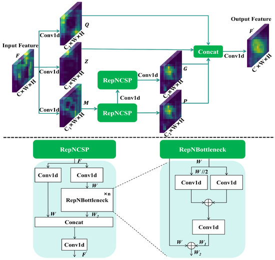
Figure 6.
Structure of RepNCSPELAN.
As shown in Figure 6, the enhanced YOLOv8s backbone network processes input features through three parallel 1 × 1 convolutional layers, adjusting the channel dimension to , and generates three intermediate feature maps: , , and . Among these, and retain the original filtered features, while is processed by a dedicated spatial feature enhancement module. This module employs multiple to progressively transform the channel dimensions into and , prouducing refined feature maps and . The spatial enhancement process strengthens the model’s focus on critical regions and improves the adaptability of spatial feature representations. Finally, a multi-channel dimensional fusion operation integrates the refined features into a globally coherent representation , enabling more effective target characterization. The overall workflow is mathematically formalized in Equations (1) and (2).
where , , and .
In the RepNCSPELAN module, the RepNCSP component enhances feature dimensionality by convolving contracted features, as detailed in Equations (3)–(5).
In the above equations, denotes the feature nodes derived from the multi-scale decomposition of high-dimensional input features. and represent the multi-scale features obtained through hierarchical scale-aware decomposition. These features are processed through stacked 1 × 1 convolutional layers to generate low-dimensional embeddings . Finally, represents the refined features obtained by integrating differential characteristics across scales, thereby enhancing representational coherence. This process ensures adaptive feature optimization while preserving essential spatial and semantic information.
2.3.2. Lightweight Multi-Dimensional Feature Network Structure Reconstruction
After being processed by the RepNCSPELAN module in the backbone network, the multi-dimensional refined features are forwarded to into the neck network. However, the original neck network lacks the capacity to effectively process multi-dimensional features. To address this issue, a novel neck architecture, termed the C-Neck (CN) network, was proposed in this study.
The proposed approach incorporates a convolutional module within the feature decoupling region to expand the receptive field of the convolutional kernels. This not only enables the capture of richer local information but also adjusts the input and output channel dimensions of the convolutional module. The original neck network adopts a progressive strategy for channel dimension adjustment. In this study, the original progressive channel dimensions were replaced with fixed values of 128 and 256 at the corresponding level. Additionally, the decoupling strategy of the convolutional modules in the up-sampling path was modified. In the Bottleneck module of the C2f structure, the transition from low-dimensional to high-dimensional representations may result in feature redundancy. To address this issue, the number of Bottleneck modules was adjusted to achieve an optimal balance for feature extraction. This approach effectively eliminates computational redundancy while consistently extracting more comprehensive and efficient features, thereby retaining a greater amount of relevant information. The specific structure of the neck network is illustrated in Figure 7, with detailed parameter specifications provided in Section 2.4.
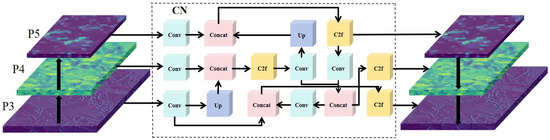
Figure 7.
The structure of the CN network.
2.3.3. Adding Semantic Feature Learning into the Detection Model
Due to interference from tomato foliage, stems, and occlusions between fruits in the greenhouse, the convolutional kernels in the neck network may encounter environmental noise when extracting image features. This results in disturbances within the feature space across channels, thereby degrading the quality of the extracted features and ultimately reducing recognition accuracy. To address this issue, the Spatial Group-wise Enhance (SGE) [37] module was introduced. The SGE module is a lightweight, channel-independent mechanism designed to generate attention factors at each spatial location within each semantic group, thus enabling dynamic adjustment of sub-features. When integrated with convolutional neural networks, it enhances feature correlations across channels, reduces the impact of noise interference in real-world scenarios, and facilitates the acquisition of comprehensive spatial and semantic information.
First, the features in the spatial domain are divided into groups. Spatial vectors are then used to represent the vectors at any position within the space. To mitigate noise interference with global spatial features, each vector in the global space undergoes a normalization process, as shown in Equations (6) and (7).
where represents an arbitrary vector in the local space, where denotes the spatial feature index , and is the set of global spatial vector feature groups. represents the spatial averaging function, and is the semantic vector of the group after normalization, approximated accordingly.
To establish the relationship between the global semantic and the normalized global features, feature enhancement is performed using the coefficients between the global semantic and the local features, as shown in Equations (8) and (9).
where represents the corresponding feature coefficient and denotes the normalized (enhanced) feature coefficient. and represent the mean and variance of the corresponding feature coefficients, respectively, and is the constant added to stabilize the coefficients.
To ensure the identity transformation of feature coefficient normalization in the network, a pair of parameters, and , are introduced, with the same number as group , to shift and scale the normalized values . Finally, the spatial vector is combined with the sigmoid function to generate the enhanced feature vector , as shown in Equations (10) and (11).
The structure of the SGE model is shown in Figure 8. SGE focuses on mapping point features to global features, significantly reducing the environmental interference in individual spatial features. This, in turn, enhances the model’s adaptability and generalization ability in complex environments.
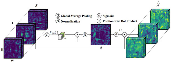
Figure 8.
The structure of the SGE model.
2.3.4. Shape_IoU Loss Function
The original YOLOv8 model employs a loss function that primarily addresses the geometric relationship between ground truth boxes and predefined anchor boxes, utilizing a shape-aware loss term to minimize their spatial discrepancies. However, this approach exhibits two critical limitations in practical agricultural detection scenarios.
For bounding box regression samples with identical nominal dimensions, subtle shape variations between anchor boxes and ground truth boxes (e.g., aspect ratio differences in tomato clusters) can disproportionately affect Intersection over Union (IoU) calculations, resulting in suboptimal localization accuracy. During the initial phases of tomato development, the chromatic similarity between immature green tomatoes and surrounding foliage induces anchor box misprioritization in the feature matching process, thereby propagating localization errors in detection outputs.
Therefore, this paper adopted Shape_IoU as the model’s edge loss function. This loss function places greater emphasis on the shape and size of the bounding boxes themselves, reducing the training loss by leveraging their properties. To address the feature insensitivity problem of the green ripe stage, the dynamic weighting of green ripe tomatoes was improved based on Shape_IoU. When the target is “T_GreenRP”, the ratio of the target to the entire image is adjusted, and the compliance value is modified to break the intrinsic value and achieve higher sensitivity. The specific formula for Shape_IoU is given by Equations (12)–(14):
where represents the scaling factor, which is related to the target size in the dataset. and represent the weighting coefficients in the horizontal and vertical directions, respectively, with their values depending on the size of the ground truth boxes. denotes the shape loss. represent the length and height of the ground truth box and the anchor box, respectively.
As shown in Figure 9, Shape_IoU gives more detailed attention to the shape and size of the anchor boxes and the ground truth bounding boxes, thereby enhancing the accuracy of bounding box regression. This enhances the model’s generalization ability and robustness in complex environments.
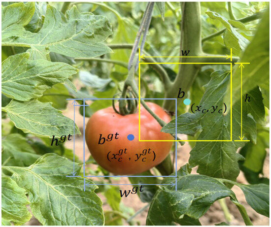
Figure 9.
Schematic diagram of Shape_IoU parameters. represents the center position of the ground truth box, denotes the center position of the anchor box, refers to the centroid coordinates of the ground truth box, and represents the centroid coordinates of the anchor box.
2.4. Network Architecture Parameters
Statistical experiments on the number of parameters and FLOPs for each network were conducted for the GCSS-YOLO (Layers [0:29]). First, for the backbone network (Layers [0:9]), replacing the RepNCSPELAN module reduced the FLOPs to 9.892 G and the number of parameters to 1.166 M. Second, the neck network (Layers [10:28]), which consisted of the proposed CN network, differed from the previous neck network. This network reduces the repetition of the C2f module, performing it only once. The input and output thresholds of the Conv module were uniformly set to 128, while those of the C2f module were changed to 128 and 256. These adjustments reduced the FLOPs of the neck network to 3.543 G and the number of parameters to 0.886 M. Lastly, for the detection head (Layers [29]), due to changes in the input and output channel thresholds in the neck network, the computational size of the previous model was reduced, with FLOPs decreasing to 7.054 G and the number of parameters to 1.262 M.
Overall, the number of layers in the network was slightly increased compared to the original model. However, computational redundancy was reduced by adjusting the feature-aware region module of the backbone network and the structure of the neck network. As a result, the computational complexity of the network was significantly reduced, providing an excellent foundation for the subsequent application in the mobile app. For specific experiments, please refer to Section 3.4 on the ablation experiment.
2.5. Deployment of the Model on a Mobile Device
To validate the performance of the improved YOLOv8s model on mobile devices, the baseline YOLOv8s model was also deployed on the mobile platform for comparison. First, the weight files (.pt files) of both models were saved. When deploying models on mobile or embedded platforms, it is typically necessary to use the model’s static graph representation, which includes the complete model files.
In light of this issue, the .pt files were converted to .onnx format to enable cross-framework compatibility. To optimize the interfering operators in the .onnx file, the onnx-simplifier tool was employed. Subsequently, the structure was converted using the NCNN framework. NCNN is an open-source, efficient neural network inference framework, specifically optimized for mobile devices. It facilitates the seamless migration of deep learning models to mobile platforms without relying on third-party dependencies, thereby promoting the efficient development of AI applications [38]. Subsequently, the .onnx format was converted into the structure (.bin) and parameter (.param) files required by the NCNN framework. Finally, the model was compiled and debugged within the Android Studio environment, and the APK file was generated for installation on Android devices. The specific application interface is shown in Figure 10.
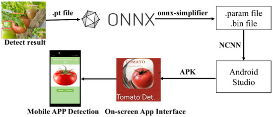
Figure 10.
App technology process flowchart.
2.6. Experiment Platform
The models in this experiment were trained and validated under the same environment. The system configuration included a 13th Gen Intel® Core™ i9-13900KF processor (Intel, Santa Clara, CA, USA), paired with an RTX 4080 GPU with 32 GB of memory (NVIDIA, Santa Clara, CA, USA). The deep learning framework used for this experiment was PyTorch (Version 2.6.0), with implementation carried out using CUDA 11.0, Python 3.8, and cuDNN version 8.0.5.39. The training parameters were set as follows: a batch size of 8, 200 iterations, an initial learning rate of 0.01, Automatic Mixed Precision (AMP) set to False, a momentum factor of 0.937, and an input image resolution of 640 × 640 pixels. All compared models were trained with identical hyperparameters. For training parameter tests, see Appendix B.
2.7. Model Evaluation Metrics
This study utilized precision (P), recall (R), mean average precision (mAP), and the F1 score to evaluate the model’s performance. mAP represents the mean of the average precision (AP) values for the detected objects, indicating the average detection precision for tomatoes at four stages of maturity. The number of parameters (Params) and the number of floating-point operations (FLOPs) were used to measure the model’s complexity. The final model’s accuracy was evaluated using metrics such as Mean Absolute Error (MAE), Root Mean Squared Error (RMSE), and the Coefficient of Determination (R2). The specific formulas for the metrics are as follows:
In the above formulas, refers to the number of tomato objects in the sample that are correctly labeled and detected by the model, denotes the number of tomatoes in the sample that the model incorrectly detects, and represents the number of tomato samples that the model fails to detect. The variable represents the total number of tomato sample categories, denotes the actual count of tomatoes, represents the number of tomatoes counted by the model, and denotes the average of the actual tomato count.
3. Experimental Results
3.1. Analysis of the Attention Modules
To mitigate the impact of environmental factors on feature extraction, attention mechanisms were incorporated to enhance the network’s ability to focus on relevant features. This section discusses various attention mechanisms and their respective contributions to enhancing feature extraction. Given the presence of tomatoes at different growth stages and varying pixel resolutions in the detected images, additional models were incorporated before the detection head, as illustrated in Figure 11.
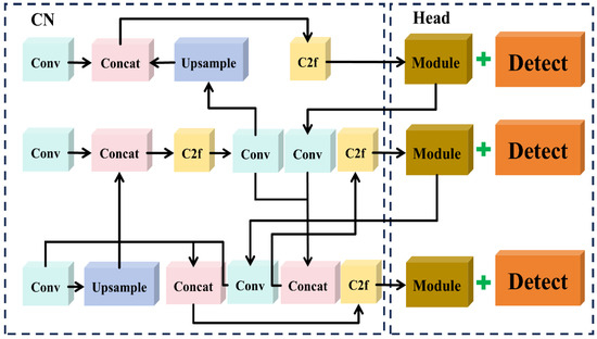
Figure 11.
The attention module integrated into the CN network.
The attention mechanism module includes TripleAttention [39], SGE, StokenAttention [40], EMAttention [41], LSK [42], and NAMAttention [43]. The experimental results are summarized in Table 2.
Table 2.
Comparison of training results of models with different attention mechanisms.
As shown in Table 2, the baseline YOLOv8s model achieved an mAP50 of 83.9%, an F1 score of 80.7%, a model size of 21.5 MB, and 28.4 GFLOPs. In terms of the mAP50, the models incorporating EMAttention, LSK, and SGE demonstrated improvements of 0.5%, 0.2%, and 0.7%, respectively, over the baseline. However, while the EMAttention module led to a 0.6% decrease in the F1 score compared to YOLOv8s, the SGE-enhanced model achieved increases of 0.2% in the mAP50 and 1.8% in the F1 score, indicating a more balanced performance improvement. The model incorporating the LSK module achieved an mAP50 that was 0.2% higher than that of the YOLOv8s baseline. However, the model with the LSK module incurred a 1.1% increase in model size and an additional 1.2 GFLOPs compared to the YOLOv8s baseline. In terms of the mAP50 and the F1 score, it underperformed relative to the SGE-enhanced model by 0.5% and 0.6%, respectively. Although the model incorporating the TripleAttention module showed no significant increases in parameter count, FLOPs, or model size compared to the YOLOv8s baseline, its mAP50 and F1 score decreased by 1.1% and 0.4%, respectively. The model incorporating the NAMAttention module achieved a 2.6% improvement in recall and a 0.2% increase in the F1 score compared to the YOLOv8s baseline. However, it also showed a 0.6% decline in the mAP50 and a 2.4% drop in precision relative to the YOLOv8s model. Finally, the model with the StokenAttention module achieved a 0.5% improvement in precision over the YOLOv8s model and a 0.4% increase compared to the SGE-based model. However, this enhancement came with a 1.04× increase in FLOPs, a 2.6 MB larger model size, and an additional 1.4 million parameters relative to YOLOv8s. Overall, the model incorporating the SGE module showed the smallest increases in model size, FLOPs, and parameter count. Additionally, its mAP50 outperformed that of the YOLOv8s model and those incorporating TripleAttention, StokenAttention, EMAttention, LSK, and NAMAttention by 0.7%, 1.8%, 5.4%, 0.2%, 0.5%, and 1.3%, respectively, achieving the best balance between model compactness and high accuracy. Therefore, the SGE module was selected for this study.
3.2. Analysis of Boundary Loss Functions
To examine the impact of boundary loss functions on the convergence of the network model, this study conducted experimental analyses using various boundary loss functions: CIoU [44], WIoU [45], MPDIoU [46], Inner_IoU [47], and Shape_IoU [48]. Since the loss function had minimal impact on the model’s complexity, experiments and discussions on the parameter count, floating-point operations, and model size were omitted. The detailed experimental data are presented in Table 3.
Table 3.
Results of the loss function performance experiment.
As shown in Table 3, introducing the Inner_IoU boundary loss function led to a 1.9% reduction in the mAP50 and a 0.6% reduction in the F1 score compared to the YOLOv8s model. After introducing the WIoU and MPDIoU boundary loss functions, the model’s F1 score improved by 0.3% and 0.5%, respectively, compared to the original loss function. When referring to the mAP50, the MPDIoU showed a 0.9% decrease compared to the original loss function, while WIoU remained unchanged but was lower than the model with Shape_IoU. Specifically, the model with Shape_IoU outperformed CIoU (by 0.2% in the mAP50 and 0.6% in the F1 score), Inner_IoU (by 2.1% in the mAP50 and 1.2% in the F1 score), MPDIoU (by 1.1% in the mAP50 and 0.3% in the F1 score), and WIoU (by 0.2% in the mAP50 and 0.1% in the F1 score). In summary, by placing greater emphasis on bounding box accuracy, the model with Shape_IoU effectively reduced interference from complex greenhouse environments, allowing it to more accurately focus on extracting tomato features.
3.3. Toward an Adaptive Experiment for Neck Networks
To verify whether the parallel channel causes different levels of imbalance compared to the adaptive channel, a comparison between the C-Neck and adaptive channel assignment modules was conducted for the target test. The experimental results are shown in Table 4. It can be observed that compared to the cross-layer channels of BiFPN, the efficient feature up-sampling of the CARAFE module and the intensive information exchange of potential semantics at different spatial scales in GFPN, C-Neck maintained a large portion of the feature surface while reducing the model size, without losing most of the features. In general, C-Neck is the most effective when the application side is the target.
Table 4.
Neck network adaptive experiment.
3.4. Ablation Experiment
The ablation study was conducted based on the original YOLOv8s model. First, the C2f module in the backbone network was replaced with the RepNCSPELAN module. Next, the original neck network was modified to the CN network. Subsequently, the SGE module was added, and, finally, the Shape_IoU loss function was incorporated into the boundary loss function. The results are shown in Table 5.
Table 5.
Ablation experiment results for each improved module.
As shown in Table 5, after replacing the C2f module in the original backbone network with the RepNCSPELAN module, the mAP50 decreased by 0.7% compared to the original model. However, the number of parameters and model size were reduced by 3.4 M and 6.6 MB, respectively, while the F1 score increased by 0.3% compared to the original YOLOv8s model. In addition, when using the CN network alone, although the mAP50 and F1 score decreased by 0.1% and 0.2%, respectively, compared to the original YOLOv8s model, it also reduced the model complexity. Subsequently, the addition of the SGE module improved the mAP50 and F1 score of the original model by 0.7% and 1.2%, respectively, indicating a reduction in the interference of environmental noise on the model’s feature extraction. After replacing the boundary loss function Shape_IoU, the mAP50 and F1 score increased by 1.2% and 1.1%, respectively, compared to the original model. This indicated that while maintaining the model size, detection precision is significantly improved. After adding the CN network in addition to replacing the RepNCSPELAN module, the number of parameters decreased by 55.9%, and the model size was reduced by 61.9% compared to the original model. Simultaneously, the model’s mAP50 and F1 score increased by 0.5% and 1.0%, respectively. This demonstrated that the CN network can more effectively process the refined multi-dimensional features. However, due to the increase in the number of layers, the model’s inference time also increased by 1.0 ms. Furthermore, when the SGE module was added in addition to this, it reduced the interference caused by environmental factors during the model’s feature processing. As a result, the mAP50 and F1 score increased by 0.4% and 0.3%, respectively, compared to the previous model, while the inference time decreased by 0.7 ms. After incorporating the lightweight boundary loss function Shape_IoU, the model achieved an mAP50 of 85.3% and an F1 score of 82.4%, representing improvements of 1.4% and 1.7%, respectively, compared to the original YOLOv8s model. Finally, the improved model reduced the number of parameters, FLOPs, and model size to 36.9%, 71.8%, and 37.2% of the original model, respectively, while also decreasing the inference time by 0.1 ms. The detailed results of the comparative experiments between the original model and the improved model for the four-stage object categories are shown in Table 6.
Table 6.
Comparison between the improved model and the original model.
The analysis was conducted based on the model optimization data. (Since the F1 score is derived from precision and recall, it was excluded from the analysis. For more details, refer to Formula (18)). The results are illustrated in Figure 12. The comprehensive analysis results indicated that the improved model achieved a higher precision across the green ripe, turning ripe, fully ripe, and disease-related decay stages. This result further validates the effectiveness of the improved modules in enhancing tomato object detection performance.
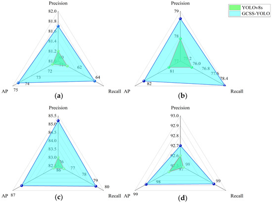
Figure 12.
Radar chart. (a) The green ripe stage. (b) The turning ripe stage. (c) The fully ripe stage. (d) The disease-related decay stage.
3.5. Detection Heatmap Analysis
To further evaluate the performance of the improved model in complex greenhouse environments, Figure 13 presents the heatmap visualizations generated using Gradient-weighted Class Activation Mapping (Grad-CAM) for both GCSS-YOLO and YOLOv8s. It is worth noting that in the heatmap visualization results, warmer colors indicate the degree of contribution of the region to the detection outcomes. The deeper the warm color, the greater the contribution of that region.
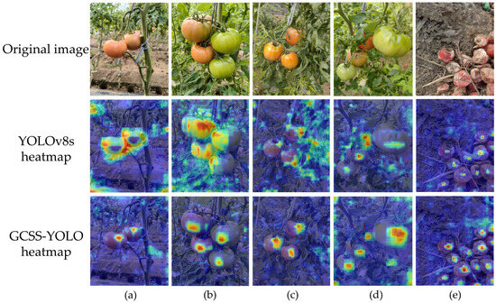
Figure 13.
Heatmap analysis of different models. (a) Minimal fruit occlusion. (b) Substantial tomato fruit occlusion. (c) Tomatoes partially occluded by branches and leaves. (d) Significant occlusion by branches and leaves. (e) Rotting tomato.
There were regions outside the target area that exhibited warm colors, as shown in Figure 13a. This suggested that the YOLOv8s model failed to effectively capture the key semantic information of the tomatoes in the spatial domain, resulting in the center of the target area displaying cool colors, while the edge regions exhibited warmer colors in the heatmap. Similarly, when the heat distribution of different parts of the tomato target in the heatmap is uneven, it indicates that the model exhibits biases during the detection process, which may lead to the omission of certain regions of the target. This is evident in Figure 13b,c. The excessive concentration of warm colors or an inconsistent warm–cool color distribution further highlights the model’s limitations in extracting representative features of tomatoes. In contrast, as shown in Figure 13d,e, although the model demonstrated some detection ability, its feature extraction capability was weaker compared to the GCSS-YOLO model. Particularly in Figure 13e, when facing tomatoes with distinct decay features, the model’s detection results exhibit color discrepancies, failing to effectively improve the model’s performance on such targets. In summary, GCSS-YOLO demonstrates stronger interpretability, better adaptability, and more robust feature extraction performance than the original model when addressing the diverse semantic characteristics of tomatoes at different ripening stages.
3.6. Comparison of Different Detection Algorithms
This study selected several widely used detection algorithms, including the single-stage SSD, YOLO series, and transformer-based RT-DETR [49] model. A comparative experiment was then conducted between these models and the improved model using the test set of a self-constructed dataset. The final results demonstrated that the improved model is effective. Specifically, the GCSS-YOLO model outperformed SSD (11.2%, 26.4%), YOLOv3 (7.7%, 10.9%), YOLOv4 (10.2%, 8.1%), YOLOv5 (2.6%, 1.5%), YOLOv7 (3.4%, 4.2%), YOLOv8 (1.4%, 1.7%), RT-DETR (6.4%, 2.4%), YOLOv9 (0.4%, 1.0%), YOLOv10 (2.4%, 1.2%), and YOLOv11 (3.7%, 2.7%) in terms of the mAP50 and F1 score. The specific performance metrics for each model are shown in Table 7.
Table 7.
Comparison of model performance.
As shown in Table 7, the YOLOv8s model surpassed most other models on the test set in terms of the mAP50 and F1 score. However, its mAP50 and F1 score values were 0.7% and 0.2% lower, respectively, than those of the YOLOv9 model, and its F1 score was 0.2% lower than the YOLOv5 model. Nevertheless, the YOLOv9 and YOLOv5 models were too large and unsuitable for deployment on mobile devices. Considering both accuracy and the need for lightweight models, the YOLOv8s model was clearly the best choice. The comparison also revealed that the SSD model achieved the highest precision among the 11 models, reaching 93.6%, which is 9% higher than that of the GCSS-YOLO model. However, due to its considerably low recall rate, the SSD model carried a high risk of missing a large number of targets during the training process. As a result, the SSD model was not suitable for the subsequent visualization experiments. In terms of the average precision, although the GCSS-YOLO model did not achieve the best performance during the green ripe stage and the disease-related decay stage, being 1.3% lower than the YOLOv9 model in the green ripe stage and 0.4% lower than the YOLOv10 model in the disease-related decay stage, it reduced the number of parameters and model size by 56.8 M and 114.4 MB compared to YOLOv9 and by 4 M and 8.6 MB compared to YOLOv10. Although the inference time of the GCSS-YOLO model was 0.1 ms longer than YOLOv11 and 0.2 ms longer than YOLOv5, its precision was significantly higher than both. Overall, the GCSS-YOLO model successfully reduces inference time and computational complexity while maintaining high precision, recall, and mAP50, demonstrating superior resource utilization efficiency and model optimization capabilities. As a result, it offers excellent advantages in handling tasks within complex environments.
To further evaluate the performance of the GCSS-YOLO model, a visualization experiment was conducted, comparing it with the models listed in Table 7, including YOLOv3, YOLOv4, YOLOv5, YOLOv7, YOLOv8, RT-DETR, YOLOv9, YOLOv10, and YOLOv11. The results of the experiment are shown in Figure 14.
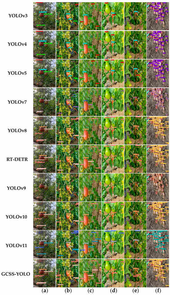
Figure 14.
Visualization results of each model: (a) The backlight conditions with multiple ripe stages coexisting. (b) The front light environment with multiple ripe stages coexisting. (c) Mild occlusion. (d) Moderate occlusion. (e) Heavy occlusion. (f) Multiple stages of disease-related decay.
From the analysis of Figure 14, it can be observed that under backlight conditions, where multiple ripe stages coexist, the YOLOv9 model missed detecting only one green ripe tomato, whereas the GCSS-YOLO model missed detecting only one turning ripe tomato. The other models exhibited varying degrees of missed detections. In the downlight environment with multiple coexisting ripeness stages, except for the GCSS-YOLO model, which missed the detection of one fully mature tomato, the other models still exhibited a significant number of missed detections. In environments with varying levels of occlusion, the GCSS-YOLO model was the only one capable of successfully detecting all the tomatoes. In contrast, the performance of the other models was hindered by the complex conditions, leading to ineffective feature extraction and missed detections. In particular, as shown in Figure 14e, the green ripe tomatoes exhibited a color remarkably similar to that of the branches and stems. In the real-world scenario, four tomatoes were present; however, most of the other models only detected one or two. The GCSS-YOLO model was the only one that effectively overcame environmental interference and accurately detected all the tomatoes. Figure 14f illustrates the excellent capability of the GCSS-YOLO model in the environment with multiple stages of disease-related decay. Compared to most of the other models, it successfully identified 35 out of a total of 38 tomatoes, despite detecting 2 fewer than the RT-DETR model. The GCSS-YOLO model demonstrated exceptional performance in accurately identifying tomatoes at various ripe stages, particularly in scenarios involving overlapping and occlusion.
Collectively, the enhanced backbone network demonstrates superior efficiency compared to previous YOLO variants: YOLOv3 (complex single-residual linking), YOLOv4 and YOLOv5 (staged feature merging), YOLOv7 (stacked channel reorganization), YOLOv8 and YOLOv11 (cross-stage residual combining), YOLOv9 (multipath reparameterization), and YOLOv10 (deep pointwise convolutional substitution). The cross-dimensional residual combination enhances feature representation while minimizing computational redundancy. Furthermore, the proposed lightweight parallel-parameter neck network outperforms recurrent neck structures in the existing models by reducing feature loss during training and improving stability. In greenhouse environments with complex interference, traditional localization loss functions (CIoU, MPDIoU, SIoU, EIoU) fail to address prediction deviations effectively. By prioritizing target-centric optimization, GCSS-YOLO significantly mitigates localization misalignment and reduces false detection rates. Overall, GCSS-YOLO achieves an optimal balance among model size, inference speed, and accuracy, surpassing existing models and providing robust support for mobile deployment in real-world scenarios.
3.7. Comparison of Different Improved Models
This study conducted comparative experiments between the proposed model and those developed in recent years within the relevant field. The selected models were chosen based on their primary focus on tomato detection, aligning with the objectives of this study, including YOLO-TGI [50], LACTA [51], and MTS-YOLO [52]. Additionally, objects with characteristics similar to tomatoes, such as apples in DNE-YOLO [21] and the Tomato Yellow Leaf Curl Virus (TYLCV) in YOLO-CDSA-BiFPN [53], were also selected for comparison. The final choice selected the SAG-YOLO model [54], which was specifically designed for wildlife detection. This choice was made due to the high diversity, complex color patterns, and distinct features exhibited by wildlife species, making this model particularly well-suited for such tasks. The comparative results of each model are presented in Table 8.
Table 8.
Comparison of experimental results for the improved model at the current stage.
By comprehensively comparing the lightweight metrics of various models, although the GCSS-YOLO model had 0.5 M more parameters, 0.7 G more FLOPs, and 0.6 MB larger model size than the LACAT model, it achieved an improvement of 1.8% in the mAP50 and 1.1% in the F1 score while reducing the processing time by 7.7 ms compared to LACAT. Compared to the lightweight YOLO-TGI model, the GCSS-YOLO model, despite an increase of 8.1 G in FLOPs and 0.4 ms in processing time, exceeded YOLO-TGI by 5% in the mAP50 and 2.6% in the F1 score. Overall, both of the aforementioned models reduced the model size excessively, neglecting essential tomato features in the process. From the perspective of precision metrics, the GCSS-YOLO model exhibited a 0.4% lower precision compared to the SAG-YOLO model, but it outperformed it by 1.7% in the mAP50 and 1.6% in the F1 score while also featuring a more lightweight model size. The GCSS-YOLO model proposed in this study demonstrates considerable advantages, achieving higher mAP50 and F1 scores compared to DNE-YOLO (by 1.3% and 1.4%, respectively), YOLO-CDSA-BiFPN (by 2.0% and 1.6%), SAG-YOLO (by 1.5% and 1.6%), MTS-YOLO (by 1.7% and 2.1%), LACTA (by 1.8% and 1.3%), and YOLO-TGI (by 5.0% and 2.6%).
Although the SAG-YOLO model was designed for multi-feature target detection, its AIFI module failed to mitigate environmental interference effectively. Additionally, the model’s overall parameter size increased significantly compared to the SGE module, which compromised its deployment efficiency. Similarly, while DNE-YOLO and YOLO-CDSA-BiFPN demonstrated partial capability in recognizing tomato-like objects, their WIOU and Inner-CIoU loss functions suffered from localization failures under environmental disturbances. Furthermore, LACTA’s AFEN feature extraction network lacked a crucial feature preservation mechanism, unlike the CN network proposed in this study, which resulted in limited robustness. The lightweight YOLO-TGI model reduced the parameters substantially but lost critical functionality in extracting tomato ripeness features. In contrast, the GCSS-YOLO framework proposed in this study achieved high-precision detection with shorter inference time, demonstrating superior performance and practicality over the existing models.
3.8. Public Dataset Validation Generalizability Test
To validate the generality and effectiveness of the improved model, this study conducted experiments using two public tomato datasets, including both regular tomatoes and cherry tomatoes. The dataset consists of 1297 images, which were split into training, validation, and test sets in a 7:2:1 ratio. The experimental setup was consistent with that described in Section 2.6. Additionally, to verify whether the improved model maintains its advantage in tomato feature extraction at a larger scale, the YOLOv8s architecture was selected for the generalization experiment. The experimental results are presented in Table 9.
Table 9.
Comparison of results between the improved model and the original model on public datasets.
It can be observed that the improved model reduced the model size by 62.6% compared to the original model, with a decrease of 8.2 G in FLOPs and a reduction of 7.1 M in the number of parameters. Although the precision was 0.3% lower than that of the original YOLOv8s model, the mAP50 was 0.2% higher, while the inference time was reduced by 1.9 ms. The fluctuations in the precision, recall, mAP50, and mAP50:95 during the training process for both models are shown in Figure 15.
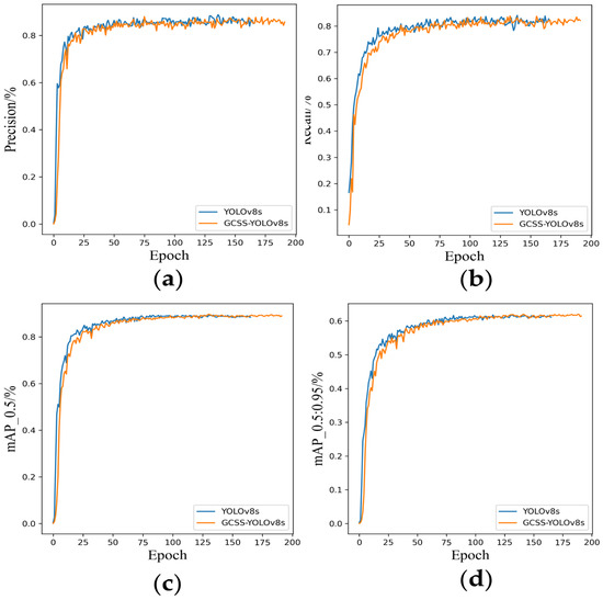
Figure 15.
Variation plots of various metrics during training. (a) The fluctuation in precision during training. (b) The fluctuation in recall during training. (c) The fluctuation in mAP50 during training, (d) The fluctuation in mAP50:95 during training.
It can be observed that the original model terminates training early to prevent overfitting, while the improved model, benefiting from greater generalization capability, continues to show a steady improvement in performance throughout training. Based on the comparative analysis above, it can be concluded that the GCSS-YOLO model performs excellently on public datasets as well. Specifically, the improved model demonstrates higher prediction confidence, fewer false positives, and a lower likelihood of false negatives, further validating the effectiveness of the proposed approach.
3.9. Generalizability Experiments in a Real Greenhouse Environment
To verify the generalization ability of the model in real-world environments, 550 tomato datasets were collected from tomato greenhouses in Liao-Zhong District, Liaoning Province, with the variety being Legend 91. The datasets were divided into training, validation, and test sets and trained according to the parameters outlined in Section 2.6. The results are shown in Table 10. The improved model achieved a lightweight design while improving the F1 score and mAP50 by 1.1% and 0.3%, respectively, compared with the original model.
Table 10.
Comparative table of generalizability tests in real greenhouse environments.
To further verify the model’s performance, the visualization results of this part of the dataset are provided in Figure 16. The visualization results are compared to the original model. As shown in Figure 16b, both of them missed the detection phenomenon, but the improved model reduced the error to a certain extent and avoided the phenomenon of missed detection and re-detection to a great extent.
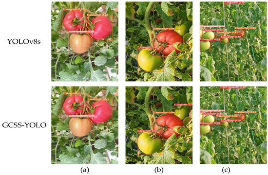
Figure 16.
Visualization of test charts in a real environment. (a) Increased testing accuracy. (b) Reduced missed tests. (c) Reduced repeated tests.
3.10. Comparison of the Application-Side Experiment
This section evaluates the application’s ability to perform high-precision detection by adding an object-counting function for the objects in the detected images. A total of 150 images from the test set and 50 real-world captured images were used for comprehensive testing, with the detection results shown in Figure 17.
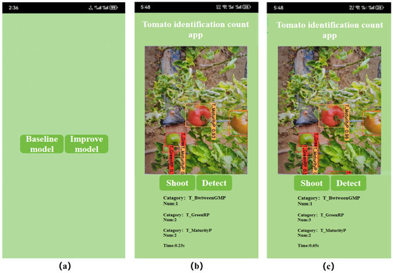
Figure 17.
Example of the app interface. (a) The interface allows users to choose between the baseline and the improved model. (b) Detection results using the improved model, showing the generated category detection count and detection time. (c) Detection results using the original model.
A statistical comparison of the predicted and actual quantities on the application side is shown in Figure 18. The horizontal axis in the figure represents the true quantities, the vertical axis represents the predicted quantities. The closer the fitted line is to the diagonal, the more accurately the model estimates the true values. Additionally, the fitted points correspond to the pairings of the true and predicted values for each quantity. It can be observed that the GCSS-YOLO model is closer to the central axis compared to the original model. Moreover, the R2 value increased by 0.0489, reaching 0.9426, indicating a better fit of the regression line. The RMSE value decreased by 0.3232, and the MAE value reduced by 0.2528, both demonstrating improvements over the original YOLOv8s model. The overall performance confirms that the application-side predictions are more accurate with the improved model.
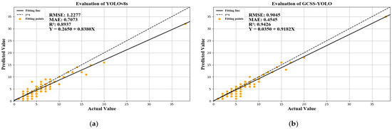
Figure 18.
Quantity statistics chart. (a) The linear statistical results of the original model. (b) The linear statistical results of the improved model.
3.11. Mobile Application Performance Experiment
3.11.1. Related Agricultural APP Function Experiment
To assess the practicality of the mobile app functionality in this study, functional comparison experiments were conducted with apps proposed by other researchers, as well as with the corresponding recognition networks. As can be seen in Table 11, although the improved model is slightly larger than most recognition networks in terms of model size, its processing time is significantly better, enhancing the timeliness of the app. Meanwhile, in terms of application functions, the app proposed in this study offers stage-by-stage counting, a function that provides convenience for subsequent precision agriculture yield estimation.
Table 11.
Comparison table of the functionality of related agricultural mobile apps.
3.11.2. Effect of Different Levels of Light and Shading on Modeling
To verify the feasibility of the improved app as well as the model in practical applications, we performed additional experiments on a partial subset of the test machine. The images were first categorized based on lighting conditions into two groups, i.e., smooth light and backlight, with 20 images each. Secondly, they were categorized according to different occlusion degrees from small to large, specifically into light occlusion, medium occlusion, and heavy occlusion, with 25 images each. These subsets were evaluated using the YOLOv8 model, the proposed GCSS-YOLO model, and the corresponding app. The analysis results are presented in Table 12.
Table 12.
Comparison table of tests with different light conditions and shading conditions.
As shown in Table 12, the experimental results demonstrate the performance patterns of the models and their associated applications under varying lighting and occlusion cases. Both models perform better under smooth lighting and light occlusion scenarios. However, in the backlight and moderate and heavy occlusion cases, YOLOv8s has a certain degree of degradation, but the GCSS-YOLO model resists the interference caused by the environment, and both mAP50 values are improved. Regarding application-level performance, the detection times for the improved model in most environments remain under 1 s, and the successful detection rates consistently exceed 90%. These results indicate greater stability and higher detection accuracy compared to the original model, further validating the improved model’s robustness and reliability in uncertain real-world environments.
4. Discussion
This study explored four ripe stages of tomatoes in a complex greenhouse environment. Drawing on recent advancements in the field of computer vision, this study proposed the GCSS-YOLO model, specifically designed for tomato detection. The model incorporated an attention mechanism, the RepNCSPELAN module, a boundary-aware loss function, and a lightweight, multi-dimensional feature fusion neck network to enhance detection performance. It is noteworthy that this study innovatively combined multi-dimensional features to enhance the precision of tomato detection. The experimental results demonstrated that with a model size of only 8.0 MB, the AP for fruits in the green ripe, turning ripe, fully ripe, and disease rot stages reached 74.5%, 82.1%, 86.8%, and 98.0%, respectively. The optimization effectively addressed the issue of color similarity between different maturity stages and surrounding complex branches and leaves while also reducing the impact of lighting and occlusion factors in the greenhouse environment on the model. When deploying the designed model to the application side, several challenges remain. In addition to detection precision, detection speed and the number of detections are equally critical. In contrast to evaluating detection speed through FPS on GPUs, this study assessed detection speed based on the time consumed during the detection process. Additionally, this study conducted a statistical analysis of tomato targets in each ripe stage using real-time detection and compared the results with those obtained using the original model. By developing a dedicated application, this research enhanced the intuitive experience for researchers, contributing to the advancement of smart agriculture, particularly in the deployment of edge devices.
Despite the promising results achieved in this study, several limitations remain. Notably, this article does not provide a comparative analysis between the default data augmentation techniques integrated within the YOLOv8 framework and the custom enhancements proposed herein. This aspect warrants further investigation and will be explored in our future work.
Meanwhile, even though the GCSS-YOLO model outperforms other models, its model size is still too large compared to the nano version. Our future research will focus on model pruning and refinement techniques to reduce computational redundancy, thereby enhancing its applicability for deployment on embedded and mobile platforms.
In addition, although the improved model improved the detection accuracy at all stages, it was lower at the green ripening stage compared to the remaining three periods of tomatoes. This is precisely because green ripening tomatoes in an actual greenhouse are too similar to the branch and leaf colors and share the same feature regions. This suggests that in future model optimization, we can minimize the environmental spatial interference, which can be dealt with by adding domain discriminators, performing adversarial training, and employing dynamic tuning strategies during the training process. In the future, we will aim to improve the accuracy and stability of the tomato classification task and ultimately improve the model’s adaptability to specific agricultural data.
5. Conclusions
To address the challenges of tomato ripe stage detection in complex greenhouse environments, this study proposes an improved, lightweight YOLOv8s detection model (GCSS-YOLO). While ensuring high precision, the model also enables real-time detection on Android devices. In this study, an image augmentation technique involving random image stitching is employed to enhance the diversity of the tomato dataset and improve the model’s generalization capability. The C2f module in the backbone network is replaced with the RepNCSPELAN module, which not only reduces the model size but also decreases the inference time. Three SGE modules are introduced in the neck network detection head to reduce the interference of environmental factors on the feature extraction channels of the model. A CN network is designed for multi-dimensional feature fusion, enabling the capture of more effective semantic information in the spatial domain. The Shape_IoU loss function is adopted to replace the original model’s convergence method, effectively addressing the challenges posed by tomato detection in real-world environments.
Based on validation conducted on a self-constructed dataset, the GCSS-YOLO model in this study achieved an accuracy of 84.6%, a recall rate of 80.3%, an mAP50 of 85.3%, and an F1 score of 82.4%. Additionally, it demonstrated a detection speed of only 2.2 ms, with 4.0 M parameters, 20.3 GFLOPs, and a model size of 8.0 MB. The improved model surpassed the current state-of-the-art models, public benchmark evaluations, and real-world experiments, which validated the model’s generalization capability across diverse scenarios. Furthermore, the algorithm was successfully implemented on mobile platforms, enabling rapid and reliable in-field detection. While this study establishes a foundation for tomato maturity recognition systems in greenhouse settings, future efforts should focus on enhancing algorithmic robustness and expanding domain-specific datasets to address edge cases. Such advancements will drive the evolution of scalable, adaptive solutions for precision agriculture, bridging the gap between theoretical research and practical agricultural automation.
Author Contributions
Conceptualization, W.Y. and H.S.; methodology, H.S.; software, H.S. and Q.Z.; validation, H.S.; formal analysis, H.S. and J.W.; investigation, H.S.; resources, C.C.; data curation, H.S., Q.Z., H.Y. and C.L.; writing—original draft preparation, H.S.; writing—review and editing, H.S.; supervision, W.Y.; project administration H.S.; funding acquisition, C.C. All authors have read and agreed to the published version of the manuscript.
Funding
This research was funded by the Liaoning Provincial Department of Education Fund, Precision Agriculture Aerospace and Smart Farm Key Technology R&D Platform Project (grant number: JYTPT2024002).
Institutional Review Board Statement
This study involved only observational data and did not involve any handling of animals; therefore, ethical approval was not required.
Data Availability Statement
The data underlying the results presented in this paper are not publicly available at this time but may be obtained from the authors upon reasonable request.
Acknowledgments
The authors would like to acknowledge Shenyang Agricultural University and Liaoning Engineering Research Center for Information Technology in Agriculture for their continuous support of our research, as well as the editors and reviewers for their careful review and valuable suggestions on this article.
Conflicts of Interest
The authors declare no conflicts of interest.
Appendix A. Cross-Domain Performance Experiment for Synthetic Datasets
In order to further verify whether the synthetic data of the disease-related decay stage would cause the model overfitting phenomenon, an incremental test of its original data and synthetic data was carried out. The specific operation process is as follows. Firstly, the test was conducted based on the original data, and, secondly, some of the synthesized tests were added sequentially in the database until they were completely increased. The final test results are shown in the table below:
As shown in Table A1, both the mAP50 and F1 scores of the model gradually increased with the addition of the synthetic dataset. Compared to the model trained solely on the original dataset, the performance improved by 5.8% in the mAP50 and 7.7% in the F1 score. Meanwhile, the mAP50 of the model stabilized when the synthetic dataset was increased by more than 90%, indicating that the addition of a moderate amount of synthetic data does not cause overfitting problems, and the addition of synthetic data improves the robustness capability of the model.
Table A1.
Synthetic dataset validation test table.
Table A1.
Synthetic dataset validation test table.
| Dataset | P/% | R/% | mAP50/% | F1 Score/% |
|---|---|---|---|---|
| Raw data | 85.7 | 90.6 | 92.7 | 88.1 |
| Raw data vs. 30% synthesized data | 88.9 | 92.2 | 94.1 | 90.5 |
| Raw data vs. 50% synthetic data | 88.4 | 93.7 | 95.7 | 91.0 |
| Raw data vs. 70% synthetic data | 90.1 | 96.5 | 97.1 | 93.2 |
| Raw data vs. 90% synthetic data | 92.8 | 97.1 | 98.2 | 94.9 |
| Raw data vs. 100% synthetic data | 92.6 | 98.1 | 98.5 | 95.8 |
Appendix B. Training Parameter Experiences
Appendix B includes information on part of the training parameters for some of the relevant tests. In preparation for training, necessary parameter screening was required. First, for the AMP test, the results are shown in Table A2. From the table, it can be seen that after turning off the AMP, the F1 score increased by 0.5% and the mAP50 increased by 0.7% compared with the original setting. Turning off the AMP reduced the processing time by 0.1 ms but made the model smoother to train and reduced the loss caused by the gradient change.
Table A2.
AMP parameter experiment.
Table A2.
AMP parameter experiment.
| Mode | P/% | R/% | mAP50/% | F1 Score/% | Inference Time/ms |
|---|---|---|---|---|---|
| AMP = True | 81.8 | 78.6 | 83.2 | 80.2 | 2.2 |
| AMP = False | 83.7 | 77.9 | 83.9 | 80.7 | 2.3 |
The detailed test results are presented in Table A3. The initial learning rate tests were conducted with Automatic Mixed Precision (AMP) disabled. The results indicate that adjusting the initial learning rate to 0.001 or increasing it to either 0.05 or 0.1 resulted in lower mAP50 and F1 scores compared to the baseline learning rate of 0.01. A learning rate that is too low can unnecessarily prolong the training process by increasing the number of required epochs. Conversely, an excessively high learning rate may cause drastic weight oscillations, overfitting, or premature convergence, ultimately compromising the model’s performance.
Table A3.
Initial learning rate parameter experimentation.
Table A3.
Initial learning rate parameter experimentation.
| Initial Learning Rate | P/% | R/% | mAP50/% | F1 Score/% |
|---|---|---|---|---|
| 0.001 | 82.2 | 78.6 | 81.7 | 80.4 |
| 0.01 | 83.7 | 77.9 | 83.9 | 80.7 |
| 0.05 | 81.7 | 78.3 | 83.1 | 80.0 |
| 0.1 | 83.9 | 77.2 | 83.7 | 80.4 |
References
- Song, J.; Kim, D.; Jeong, E.; Park, J. Determination of Optimal Dataset Characteristics for Improving YOLO Performance in Agricultural Object Detection. Agriculture 2025, 15, 731. [Google Scholar] [CrossRef]
- Cama-Pinto, D.; Damas, M.; Holgado-Terriza, J.A.; Gómez-Mula, F.; Cama-Pinto, A. Path Loss Determination Using Linear and Cubic Regression Inside a Classic Tomato Greenhouse. Int. J. Environ. Res. Public Health 2019, 16, 1744. [Google Scholar] [CrossRef] [PubMed]
- Meng, Z.; Du, X.; Xia, J.; Ma, Z.; Zhang, T. Real-time statistical algorithm for cherry tomatoes with different ripeness based on depth information mapping. Comput. Electron. Agric. 2024, 220, 108900. [Google Scholar] [CrossRef]
- Yu, F.; Bai, J.; Fang, J.; Guo, S.; Zhu, S.; Xu, T. Integration of a Parameter Combination Discriminator Improves the Accuracy of Chlorophyll Inversion from Spectral Imaging of Rice. Agric. Commun. 2024, 2, 100055. [Google Scholar] [CrossRef]
- Yue, X.; Qi, K.; Na, X.; Zhang, Y.; Liu, Y.; Liu, C. Improved YOLOv8-Seg Network for Instance Segmentation of Healthy and Diseased Tomato Plants in the Growth Stage. Agriculture 2023, 13, 1643. [Google Scholar] [CrossRef]
- Yue, J.; Li, T.; Feng, H.; Fu, Y.; Liu, Y.; Tian, J.; Yang, H.; Yang, G. Enhancing Field Soil Moisture Content Monitoring Using Laboratory-Based Soil Spectral Measurements and Radiative Transfer Models. Agric. Commun. 2024, 2, 100060. [Google Scholar] [CrossRef]
- He, K.; Gkioxari, G.; Dollár, P.; Girshick, R. Mask r-cnn. In Proceedings of the IEEE International Conference on Computer Vision, Venice, Italy, 22–29 October 2017; pp. 2961–2969. [Google Scholar]
- Ren, S.; He, K.; Girshick, R.; Sun, J. Faster R-CNN: Towards Real-Time Object Detection with Region Proposal Networks. IEEE Trans. Pattern Anal. Mach. Intell. 2017, 39, 1137–1149. [Google Scholar] [CrossRef]
- Wang, Z.; Ling, Y.; Wang, X.; Meng, D.; Nie, L.; An, G.; Wang, X. An improved Faster R-CNN model for multi-object tomato maturity detection in complex scenarios. Ecol. Inform. 2022, 72, 101886. [Google Scholar] [CrossRef]
- Zu, L.; Zhao, Y.; Liu, J.; Su, F.; Zhang, Y.; Liu, P. Detection and Segmentation of Mature Green Tomatoes Based on Mask R-CNN with Automatic Image Acquisition Approach. Sensors 2021, 21, 7842. [Google Scholar] [CrossRef]
- Minagawa, D.; Kim, J. Prediction of Harvest Time of Tomato Using Mask R-CNN. AgriEngineering 2022, 4, 356–366. [Google Scholar] [CrossRef]
- Redmon, J.; Farhadi, A. YOLOv3: An Incremental Improvement. arXiv 2018, arXiv:1804.02767. [Google Scholar]
- Bochkovskiy, A.; Wang, C.-Y.; Liao, H.-Y.M. YOLOv4: Optimal Speed and Accuracy of Object Detection. arXiv 2020, arXiv:2004.10934. [Google Scholar]
- Hussain, M. YOLOv5, YOLOv8 and YOLOv10: The Go-To Detectors for Real-time Vision. arXiv 2024, arXiv:2407.02988. [Google Scholar]
- Wang, C.; Bochkovskiy, A.; Liao, H.-Y.M. YOLOv7: Trainable Bag-of-Freebies Sets New State-of-the-Art for Real-Time Object Detectors. In Proceedings of the IEEE/CVF Conference on Computer Vision and Pattern Recognition (CVPR), Vancouver, BC, Canada, 17–24 June 2023; pp. 7464–7475. [Google Scholar] [CrossRef]
- Varghese, R.; Sambath, M. YOLOv8: A Novel Object Detection Algorithm with Enhanced Performance and Robustness. In Proceedings of the 2024 International Conference on Advances in Data Engineering and Intelligent Computing Systems, Chennai, India, 18–19 April 2024; pp. 1–6. [Google Scholar] [CrossRef]
- Wang, C.Y.; Yeh, I.H.; Liao, H.-Y.M. YOLOv9: Learning What You Want to Learn Using Programmable Gradient Information. arXiv 2024, arXiv:2402.13616. [Google Scholar]
- Wang, A.; Chen, H.; Liu, L.; Chen, K.; Lin, Z.; Han, J.; Ding, G. YOLOv10: Real-Time End-to-End Object Detection. arXiv 2024, arXiv:2405.14458. [Google Scholar]
- Khanam, R.; Hussain, M. YOLOv11: An Overview of the Key Architectural Enhancements. arXiv 2024, arXiv:2410.17725. [Google Scholar]
- Liu, J.; Wang, X. EggplantDet: An efficient lightweight model for eggplant disease detection. Alex. Eng. J. 2025, 115, 308–323. [Google Scholar] [CrossRef]
- Wu, H.; Mo, X.; Wen, S.; Wu, K.; Ye, Y.; Wang, Y.; Zhang, Y. DNE-YOLO: A method for apple fruit detection in Diverse Natural Environments. J. King Saud. Univ.—Comput. Inf. Sci. 2024, 36, 102220. [Google Scholar] [CrossRef]
- Zhu, R.; Hao, F.; Ma, D. Research on Polygon Pest-Infected Leaf Region Detection Based on YOLOv8. Agriculture 2023, 13, 2253. [Google Scholar] [CrossRef]
- Paul, A.; Machavaram, R.; Ambuj; Kumar, D.; Nagar, H. Smart Solutions for Capsicum Harvesting: Unleashing the Power of YOLO for Detection, Segmentation, Growth Stage Classification, Counting, and Real-Time Mobile Identification. Comput. Electron. Agric. 2024, 219, 108832. [Google Scholar] [CrossRef]
- Ren, R.; Zhang, S.; Sun, H.; Wang, N.; Yang, S.; Zhao, H.; Xin, M. YOLO-RCS: A method for detecting phenological period of ‘Yuluxiang’ pear in unstructured environment. Comput. Electron. Agric. 2025, 229, 109819. [Google Scholar] [CrossRef]
- Zhu, X.; Chen, F.; Zheng, Y.; Chen, C.; Peng, X. Detection of Camellia oleifera fruit maturity in orchards based on modified lightweight YOLO. Comput. Electron. Agric. 2024, 226, 109471. [Google Scholar] [CrossRef]
- Yang, G.; Wang, J.; Nie, Z.; Yang, H.; Yu, S. A Lightweight YOLOv8 Tomato Detection Algorithm Combining Feature Enhancement and Attention. Agronomy 2023, 13, 1824. [Google Scholar] [CrossRef]
- Gao, G.H.; Shuai, C.Y.; Wang, S.Y.; Ding, T. Using improved YOLO V5s to recognize tomatoes in a continuous working environment. Signal Image Video Process. 2024, 18, 4019–4028. [Google Scholar] [CrossRef]
- Sun, X.Y. Enhanced tomato detection in greenhouse environments: A lightweight model based on S-YOLO with high accuracy. Front. Plant Sci. 2024, 15, 1451018. [Google Scholar] [CrossRef]
- Chen, W.; Liu, M.; Zhao, C.; Li, X.; Wang, Y. MTD-YOLO: Multi-task deep convolutional neural network for cherry tomato fruit bunch maturity detection. Comput. Electron. Agric. 2024, 216, 108533. [Google Scholar] [CrossRef]
- Liao, J.; He, X.; Liang, Y.; Wang, H.; Zeng, H.; Luo, X.; Li, X.; Zhang, L.; Xing, H.; Zang, Y. A Lightweight Cotton Verticillium Wilt Hazard Level Real-Time Assessment System Based on an Improved YOLOv10n Model. Agriculture 2024, 14, 1617. [Google Scholar] [CrossRef]
- Li, Y.; Chen, X.; Yin, L.; Hu, Y. Deep Learning-Based Methods for Multi-Class Rice Disease Detection Using Plant Images. Agronomy 2024, 14, 1879. [Google Scholar] [CrossRef]
- Tao, Z.; Li, K.; Rao, Y.; Li, W.; Zhu, J. Strawberry Maturity Recognition Based on Improved YOLOv5. Agronomy 2024, 14, 460. [Google Scholar] [CrossRef]
- Yu, C.; Feng, J.; Zheng, Z.; Guo, J.; Hu, Y. A Lightweight SOD-YOLOv5n Model-Based Winter Jujube Detection and Counting Method Deployed on Android. Comput. Electron. Agric. 2024, 218, 108701. [Google Scholar] [CrossRef]
- Chen, C.; Zheng, Z.; Xu, T.; Guo, S.; Feng, S.; Yao, W.; Lan, Y. YOLO-Based UAV Technology: A Review of the Research and Its Applications. Drones 2023, 7, 190. [Google Scholar] [CrossRef]
- Li, J.; Qiao, Y.; Liu, S.; Zhang, J.; Yang, Z.; Wang, M. An Improved YOLOv5-Based Vegetable Disease Detection Method. Comput. Electron. Agric. 2022, 202, 107345. [Google Scholar] [CrossRef]
- Liu, Y.H.; Huang, Z.H.; Song, Q.; Bai, K. PV-YOLO: A lightweight pedestrian and vehicle detection model based on improved YOLOv8. Digit. Signal Process. 2025, 156, 104857. [Google Scholar] [CrossRef]
- Li, X.; Hu, X.; Yang, J. Spatial Group-wise Enhance: Improving Semantic Feature Learning in Convolutional Networks. arXiv 2019, arXiv:1905.09646. [Google Scholar]
- Zaferani, H.; Kiani, K.; Rastgoo, R. Real-Time Face Verification on Mobile Devices Using Margin Distillation. Multimed. Tools Appl. 2023, 82, 44155–44173. [Google Scholar] [CrossRef]
- Misra, D.; Nalamada, T.; Arasanipalai, A.U.; Hou, Q. Rotate to Attend: Convolutional Triplet Attention Module. arXiv 2020, arXiv:2010.03045. [Google Scholar]
- Huang, H.; Zhou, X.; Cao, J.; He, R.; Tan, T. Vision Transformer with Super Token Sampling. arXiv 2024, arXiv:2211.11167. [Google Scholar]
- Ouyang, D.; He, S.; Zhang, G.; Luo, M.; Guo, H.; Zhan, J.; Huang, Z. Efficient Multi-Scale Attention Module with Cross-Spatial Learning. arXiv 2023, arXiv:2305.13563. [Google Scholar]
- Li, Y.; Hou, Q.; Zheng, Z.; Cheng, M.-M.; Yang, J.; Li, X. Large Selective Kernel Network for Remote Sensing Object Detection. arXiv 2024, arXiv:2303.09030. [Google Scholar]
- Liu, Y.; Shao, Z.; Teng, Y.; Hoffmann, N. NAM: Normalization-based Attention Module. arXiv 2021, arXiv:2111.12419. [Google Scholar]
- Zheng, Z.; Wang, P.; Liu, W.; Li, J.; Ye, R.; Ren, D. Distance-IoU Loss: Faster and Better Learning for Bounding Box Regression. Proc. AAAI Conf. Artif. Intell. 2020, 34, 12993–13000. [Google Scholar] [CrossRef]
- Tong, Z.; Chen, Y.; Xu, Z.; Yu, R. Wise-IoU: Bounding Box Regression Loss with Dynamic Focusing Mechanism. arXiv 2023, arXiv:2301.10051. [Google Scholar]
- Ma, S.; Xu, Y. MPDIoU: A Loss for Efficient and Accurate Bounding Box Regression. arXiv 2023, arXiv:2307.07662. [Google Scholar]
- Zhang, H.; Xu, C.; Zhang, S. Inner-IoU: More Effective Intersection over Union Loss with Auxiliary Bounding Box. arXiv 2023, arXiv:2311.02877. [Google Scholar]
- Zhang, H.; Zhang, S. Shape-IoU: More Accurate Metric considering Bounding Box Shape and Scale. arXiv 2024, arXiv:2312.17663. [Google Scholar]
- Zhao, Y.; Lv, W.; Xu, S.; Wei, J.; Wang, G.; Dang, Q.; Liu, Y.; Chen, J. DETRs Beat YOLOs on Real-Time Object Detection. In Proceedings of the 2024 IEEE/CVF Conference on Computer Vision and Pattern Recognition (CVPR), Seattle, WA, USA, 16–22 June 2024; Volume 35, pp. 16965–16974. [Google Scholar] [CrossRef]
- Kang, R.; Huang, J.; Zhou, X.; Ren, N.; Sun, S. Toward Real Scenery: A Lightweight Tomato Growth Inspection Algorithm for Leaf Disease Detection and Fruit Counting. Plant Phenomics 2024, 6, 0174. [Google Scholar] [CrossRef]
- Gao, J.; Zhang, J.; Zhang, F.; Gao, J. LACTA: A Lightweight and Accurate Algorithm for Cherry Tomato Detection in Unstructured Environments. Expert. Syst. Appl. 2024, 238, 122073. [Google Scholar] [CrossRef]
- Wu, M.; Lin, H.; Shi, X.; Zhu, S.; Zheng, B. MTS-YOLO: A Multi-Task Lightweight and Efficient Model for Tomato Fruit Bunch Maturity and Stem Detection. Horticulturae 2024, 10, 1006. [Google Scholar] [CrossRef]
- Mo, H.; Wei, L. Tomato Yellow Leaf Curl Virus Detection Based on Cross-Domain Shared Attention and Enhanced BiFPN. Ecol. Inform. 2024, 85, 102912. [Google Scholar] [CrossRef]
- Chen, L.; Li, G.; Zhang, S.; Mao, W.; Zhang, M. YOLO-SAG: An Improved Wildlife Object Detection Algorithm Based on YOLOv8n. Ecol. Inform. 2024, 83, 102791. [Google Scholar] [CrossRef]
Disclaimer/Publisher’s Note: The statements, opinions and data contained in all publications are solely those of the individual author(s) and contributor(s) and not of MDPI and/or the editor(s). MDPI and/or the editor(s) disclaim responsibility for any injury to people or property resulting from any ideas, methods, instructions or products referred to in the content. |
© 2025 by the authors. Licensee MDPI, Basel, Switzerland. This article is an open access article distributed under the terms and conditions of the Creative Commons Attribution (CC BY) license (https://creativecommons.org/licenses/by/4.0/).