Factors Influencing the Spatial Distribution of Soil Total Phosphorus Based on Structural Equation Modeling

Abstract

Soil total phosphorus plays an important role in soil fertility, plant growth, and bioge-ochemical cycles. This study aims to determine the spatial distribution characteristics of soil total phosphorus and identify its main influencing factors in the study area, thereby providing a basis for the scientific management of soil total phosphorus. Here, we conducted a comprehensive analysis by combining classical statistical analysis, ge-ostatistics methods, Pearson correlation analysis, one-way analysis of variance (ANOVA), and structural equation modeling (SEM) to explore the spatial distribution patterns of soil total phosphorus and its influencing factors. The results showed that soil total phosphorus in the study area ranged from 161.00 to 991.00 mg/kg, with an average of 495.71 mg/kg. Spatially, soil total phosphorus exhibited a patchy distribu-tion pattern, with high values primarily concentrated in cultivated areas along rivers and low values mainly located in forested areas in the southeastern and central re-gions. Additionally, the nugget effect of soil total phosphorus was 71.5%, indicating a moderate level of spatial variability. The Pearson correlation analysis revealed that soil total phosphorus content was significantly correlated with multiple factors, including land use types, soil parent material, distance from settlements, slope, and soil pH. Based on these findings, we employed ANOVA to analyze the impacts of various fac-tors. The results indicated that soil total phosphorus content showed significant differences under the influence of different factors. Subsequently, we further explored in depth the action paths through which these factors affect soil total phosphorus us-ing SEM. The SEM results showed that the absolute values of the total effects of the influencing factors on soil total phosphorus, ranked from highest to lowest, were as follows: land use types (0.499) > soil parent material (0.240) > distance from settle-ments (0.178) > slope (0.161) > elevation (0.127) > soil pH (0.114) > normalized differ-ence vegetation index (0.103). These findings provide a scientific foundation for the effective management of soil total phosphorus in similar study areas.

1. Introduction

Phosphorus is an essential nutrient for plants, and moderate phosphorus content in soil is crucial for crop growth [1]. Nevertheless, excessive soil total phosphorus content can lead to a series of negative impacts. On the one hand, excessive accumulation of phosphorus in the soil can easily disrupt the ecological balance of the soil [2]. On the other hand, under the influence of rainfall, irrigation, and other hydrological processes, excess phosphorus in the soil may enter water bodies through runoff, seepage, and erosion, gradually accumulating and ultimately leading to water eutrophication [3,4]. For example, studies have shown that approximately 3–4.3 × 10⁶ tons of phosphorus are lost from soil to water bodies worldwide each year [5]. However, soil total phosphorus is influenced by factors such as soil parent material, climate, organisms, and topography, resulting in significant spatial heterogeneity in its distribution [6,7,8]. Therefore, it is of great significance to clarify the spatial differentiation patterns and driving mechanism of soil total phosphorus for the scientific management of soil total phosphorus, to effectively coordinate agricultural production and sustainable environmental development [9].

Previous studies have used traditional analysis methods to explore the spatial distribution of soil total phosphorus and its influencing factors [10,11]. For example, Li et al. [12] used general statistics and one-way analysis of variance (ANOVA) to find that soil total phosphorus content in the topsoil of farmland in the Chengdu Plain was affected by the agricultural land-use changes and soil parent material. Zhu et al. [13] applied linear regression to analyze forests in China and found that the main factor affecting the distribution of soil total phosphorus was the interaction between temperature and precipitation. Han et al. [14] used GeoDetector for analysis and found that soil erosion, elevation, particle size, and soil pH were the influencing factors affecting the soil total phosphorus content in the Nanliao River Basin. However, traditional analytical methods have limited capacity to capture nonlinear relationships, which may lead to a misunderstanding or underestimation of some influencing factors. In recent years, the introduction of geostatistics has provided a reliable data foundation for studying the spatial heterogeneity of soil properties [15,16]. Moreover, structural equation modeling (SEM), which integrates both direct and indirect effects and reveals causal pathways, provides a new idea for studying the mechanism of spatial differentiation of soil nutrients [17,18].

Poyang Lake, as a typical river-connected lake located in the middle and lower reaches of the Yangtze River, plays an important role in maintaining the ecological balance and sustainable development of its freshwater resources and wetland systems [19]. Studies have shown that in recent years, the total phosphorus concentration in Poyang Lake has been rising, posing severe challenges to water body eutrophication [20,21]. Against this backdrop, Jiangxi Province has issued the Regulation on the Prevention and Control of Total Phosphorus Pollution in the Poyang Lake Basin, aimed to reduce the average total phosphorus concentration in the Lake to reach the standard of Lake Reservoir Class III by 2030 (total phosphorus ≤ 0.2 mg/L), and encourages the purification of farmland drainage and surface runoff [22]. Therefore, it is of practical significance to control the total phosphorus content of the soil to promote the prevention and control of total phosphorus in the Poyang Lake Basin.

Therefore, we selected the Haihunjiang River Basin, a typical small watershed in the Poyang Lake Basin, as the study area. We propose the following assumptions: (1) the soil total phosphorus content in the study area exhibits significant spatial heterogeneity; (2) the spatial distribution of soil total phosphorus is influenced by natural factors (eg., soil parent material type, topographic conditions), soil physicochemical properties (eg., pH value, bulk density) and human activities (eg., land use type, distance from settlements). To explore the spatial distribution pattern and driving mechanism of soil total phosphorus in the study, we integrated classical statistics, geostatistics, and structural equation model (SEM) to construct a multi-level analysis framework for in-depth analysis. This study aims to achieve the following goals: (1) comprehensively reveal the spatial heterogeneity and distribution of soil total phosphorus; (2) quantitative identification of the factors affecting the spatial distribution of soil total phosphorus and its action path. The research results will not only provide a scientific basis for optimizing soil total phosphorus management strategy in the study area but also provide theoretical support for soil nutrient management and non-point source pollution prevention and control in similar watersheds. This is of great significance for promoting the coordinated development of regional sustainable agriculture and ecological environment protection.

2. Materials and Methods

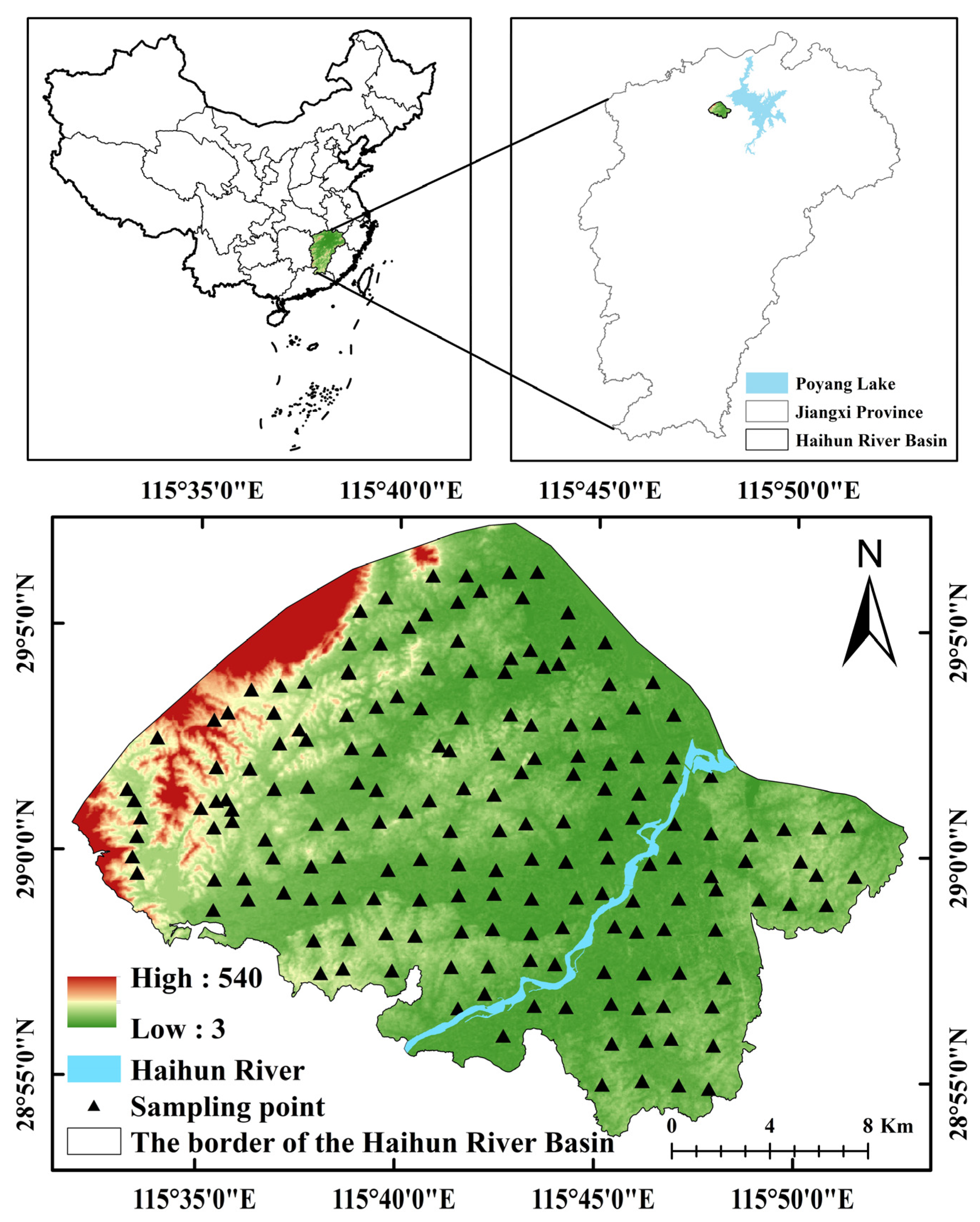
2.1. Overview of the Study Area

Haihunjiang River Basin is located in the southern part of Yongxiu County, Jiangxi Province, China, with a longitude of 115°31′–115°52′ E and a latitude of 28°53′–29°07′ N, covering an area of 466.51 km². This area belongs to the transitional zone between the central and northern subtropical regions, with a humid climate, high temperature and sunshine, and distinct four seasons. Its terrain is flat, mainly consisting of plains, with the highest and lowest elevations of 540 m and 3 m respectively (Figure 1).

2.2. Soil Sample Collection and Processing

In this study, we collected 180 surface soil sampling points (0–20 cm) in the study area in October 2022 (Figure 1). Considering the uniform spatial distribution and the representativeness of sampling points, we adopted the “X” (five-point) sampling method to select appropriate plots for sampling within a regular grid of 1.5 km × 1.5 km [23]. In the field, we broke soil clods by hand; picked out impurities such as roots, stones, and insect bodies; and after thorough mixing, retained 1 kg of soil samples for each point. Meanwhile, we recorded information such as the longitude and latitude, land use types, soil types, and cultivation conditions of sampling points. The air-dried soil samples underwent standardized pretreatment procedures including grinding and sieving. The determination of soil total phosphorus and soil pH was carried out in strict accordance with the standard method: the total phosphorus content was determined by digestion-molybdenum-antimony anti-spectrophotometry (YTP-6T, Beijing Yuangui Instrument Technology Co., Beijing, China), and the soil pH was determined by the potentiometric method (PHS-3C, INESA Scientific Instrument Co., Shanghai, China).

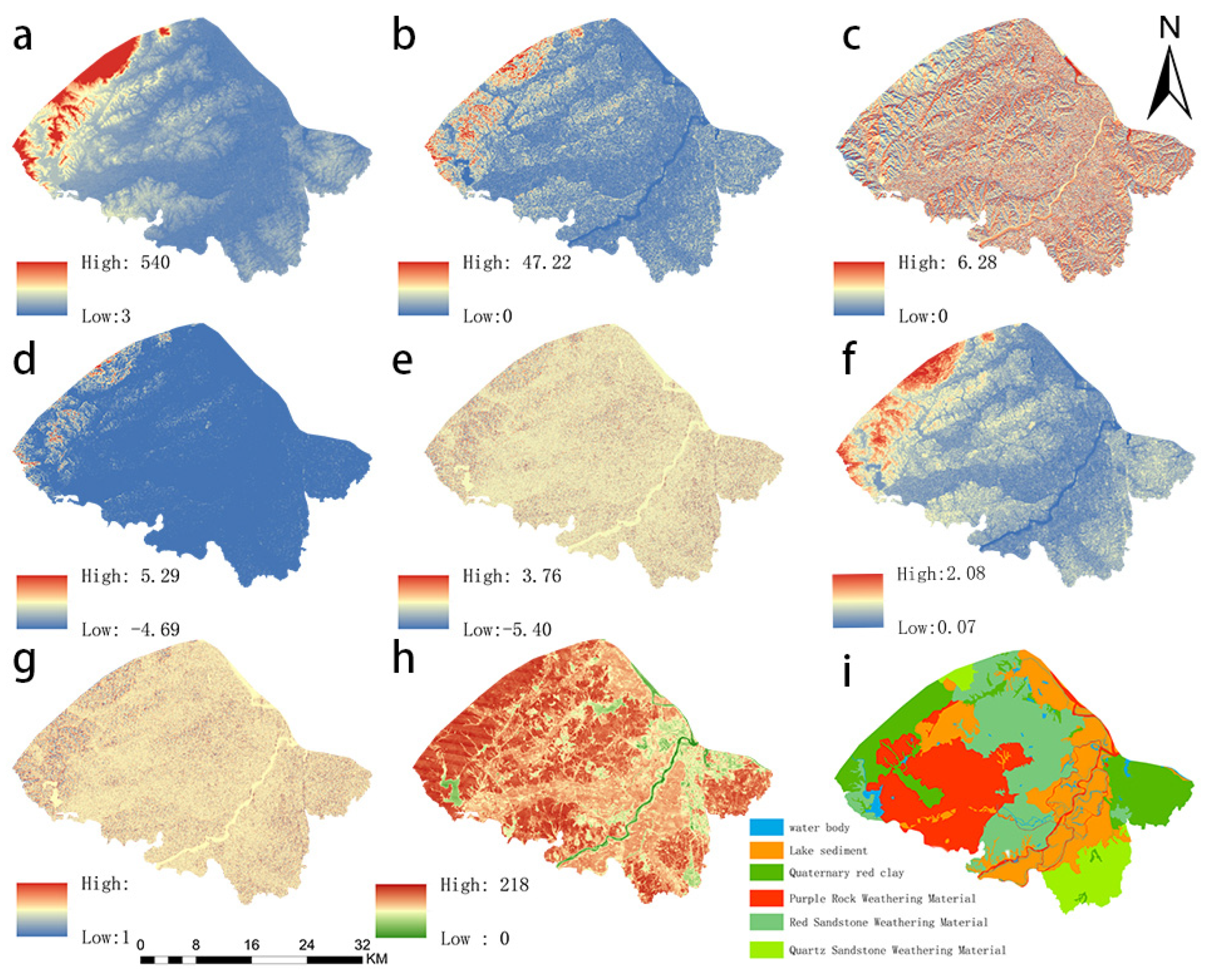
2.3. Data Sources and Data Processing

Land use types and soil physicochemical properties were obtained from sampling surveys, while soil parent material data were obtained from the second soil census data (https://www.resdc.cn/, accessed on 23 June 2024). Additionally, topographic factors including elevation, slope, aspect, plan curvature, profile curvature, surface roughness, and topographic position index (TPI) were derived from digital elevation model (DEM) data (https://www.gscloud.cn/, accessed on 23 June 2024). These factors were calculated using ArcGIS 10.7 [24]. For the normalized difference vegetation index (NDVI) data, we utilized Landsat 8 OLI remote-sensing imagery (https://www.gscloud.cn/, accessed on 23 June 2024). NDVI values were calculated after radiometric calibration and atmospheric correction using ENVI 5.3 [25] (Figure 2). The mean ± 3 times standard deviation (Lajda criterion method) was used to identify outliers, i.e., the normal data range was considered to be between [μ − 3σ, μ + 3σ] (where μ is the mean value of the original sample data and σ is the standard deviation of the original sample data), beyond which outliers were recognized as outliers and were rejected [26]. After excluding outliers, 174 soil total phosphorus sampling points were finally determined for the subsequent analysis of this study. The raw data were summarized and organized using Excel 2019, while descriptive statistics, correlation analysis, ANOVA, and corresponding graphs were produced using SPSS 27 and Origin 2022. According to Zhang’s study [27], the natural breakpoint method was used to discretize the factors of elevation, slope, and distance from rivers, ditches, and settlements into 5 categories. Regarding the soil pH, which ranges from 3.7 to 7.19, dividing it into five categories would have resulted in insufficient data points in some intervals, failing to provide sufficient support for effective analysis. Therefore, soil pH was classified into four categories in this study (Table S1).

2.4. Research Methodology

2.4.1. Classical Statistics

This study conducted a classical statistical analysis based on the data from 174 soil total phosphorus sampling points. First, we characterized the data distribution features using extreme values, the mean, the median, and the standard deviation. Then, we employed the coefficient of variation (CV) to quantify the intensity of spatial variation (CV ≤ 10% indicates weak variation, 10% < CV ≤ 100% indicates moderate variation, and CV > 100% indicates strong variation) [28]. Moreover, we applied the Kolmogorov–Smirnov (K–S) test to assess the normality of the data distribution, thus providing a statistical foundation for the subsequent correlation analysis [29].

2.4.2. Geostatistics

The Moran’s index was chosen to represent the spatial autocorrelation of soil total phosphorus, aiming to quantify its degree of the spatial correlation [30]. The Moran index, in the narrow sense, is a rational number that is normalized between values after variance normalization, and some values outside this range are also calculated using the following formula:

$$I={\displaystyle \frac{n}{S_0}}{\displaystyle \frac{{\displaystyle \sum _{i=1}^n{\displaystyle \sum _{j=1}^n{w}_{i,j}}}{z}_i{z}_j}{{\displaystyle \sum _{i=1}^n{z}_i^2}}}$$

(1)

where $I$ is the value of Moran’s index, $Z_{\mathrm{i}}$ is the deviation of the attribute of the element, $i$ from its mean value, $w_{i,j}$ is the spatial weight between the element $i$ and $j$, $n$ is equal to the total number of elements, and $S_0$ is the aggregation of all the spatial weights.

A Moran’s I > 0 indicates a positive spatial correlation; the larger the value, the more pronounced the spatial correlation. Moran’s I < 0 indicates a negative spatial correlation; the smaller the value, the greater the spatial variance; otherwise, Moran’s I = 0 indicates that the spatial correlation is random.

The semi-variogram is a key function in geostatistics for the study of soil variability and is mainly used to describe the degree of difference in spatial attribute variables objectively [31]. We fitted various semi-variogram models using GS+9.0 software to identify the best-fitting model. The calculation formula is as follows:

$$\gamma (h)={\displaystyle \frac{1}{2N(h)}}{\displaystyle \sum _{a=1}^{N(h)}\left[z({\mu }_a)-z({\mu }_a+h)\right]}$$

(2)

where $\gamma \left(h\right)$ is the semivariance value, $h$ is the interval distance between two points, $z\left({\mu }_a\right)$ and $z\left({\mu }_a+h\right)$, $z\left({\mu }_a\right)$ is the standardized values of ${\mu }_a$, $z\left({\mu }_a+h\right)$ is the standardized values of ${\mu }_a+h$, $N\left(h\right)$ is the number of all the sample pairs in $h$, and $a$ is the index, from 1 to $N\left(h\right)$.

The main parameters of the semivariogram include the fitting coefficient $r^2$, nugget value $C_0$, and abutment value $\left(C_0+C\right)$. Among them, the nugget represents random variation, the abutment value represents the total variation caused by the random and structural factors, and the ratio of the nugget value to the abutment value ($C_0/\left(C_0+C\right)$) indicates the degree of spatial correlation of the system variables. It is usually considered to be stronger when the ratio is <25%; when the ratio is in the range of 25% to 75%, the system indicates moderate spatial correlation; and when the proportion is >75%, it indicates a weak spatial correlation of the system [31]. The range represents the maximum distance of the spatial autocorrelation among the sampling points.

We used the Kriging interpolation method to map the spatial distribution of soil total phosphorus in the study area. This method uses sampling points data and the structure of the variogram to provide the best linear unbiased estimation of the soil total phosphorus content at unsampled locations. Compared with other interpolation methods, the Kriging interpolation method fully takes into account the spatial locations of sample points and their spatial relationships with each other, which can effectively improve the interpolation accuracy [32]. The calculation formula is as follows:

$$\widehat{Z}(x_0)={\displaystyle \sum _{i=1}^n{\lambda }_i}Z(x_i)$$

(3)

where $\widehat{Z}(x_0)$ represents the interpolation result at the interpolation point $x_0$; $Z(x_i)$ is the measured value at the measured point $x_i$; $n$ is the number of measured points involved in the calculation; and ${\lambda }_i$ is the Kriging weight coefficient, which is obtained from the variogram rather than the distance between the measured point and the interpolation point. To ensure unbiased estimation, the sum of the weights is 1.

2.4.3. Method of Influencing Factor Analysis

We comprehensively applied a variety of methods to deeply analyze the relationships among various factors. First, we used Pearson correlation analysis to initially screen out the factors closely related to the soil total phosphorus content. Then, we employed ANOVA to further explore the differences in the impacts of the screened influencing factors on the soil total phosphorus content. Finally, we constructed an SEM to evaluate the comprehensive impact paths and effect magnitudes of various factors on the soil total phosphorus content, revealing the potential causal relationships and systematically and accurately explaining the influencing mechanism of the soil total phosphorus content.

The Pearson coefficient correlation analysis method was used to determine the degree of correlation between soil total phosphorus and influencing factors [33]. The factors selected were topographic, physicochemical properties, and anthropogenic factors. The topographic factors include elevation, slope, aspect, slope curvature, plane curvature, TPI, and surface roughness. The physicochemical properties were bulk density, soil pH, and soil parent material, and the anthropogenic factors included land use type, NDVI, distance from rivers, distance from ditches, and distance from settlements. The Pearson correlation coefficient of <0 and >0 indicated negative and positive correlations. The formula for Pearson’s correlation coefficient is as follows:

$$\mathrm{r}={\displaystyle \frac{{\displaystyle {\sum }_{a=1}^n\left(X_a-\overline{X}\right)\left(Y_a-\overline{Y}\right)}}{\sqrt{{\displaystyle {\sum }_{a=1}^n{\left(X_a-\overline{X}\right)}^2}}\sqrt{{\displaystyle {\sum }_{a=1}^n{\left(Y_a-\overline{Y}\right)}^2}}}}$$

(4)

where $r$ represents the Pearson correlation coefficient; $\overline{X}$ and $\overline{Y}$ are the sample means of the samples $X_a$ and $Y_a$, respectively; and $n$ is the number of observed objects.

ANOVA is mainly used to test whether there are significant differences in the mean values of soil total phosphorus content under different levels of a single factor [34]. Additionally, SEM is a theory-driven, confirmatory statistical method that reveals latent mechanisms by testing the hypothesized causal relationships among variables [35]. In this study, we used the Amos 27 with the maximum likelihood method for SEM analysis. The path coefficient outputs from the model were used to analyze the different effects between the variables, and the effects were decomposed into direct, indirect, and total effects. The direct effect reflects the direct influence between variables. The indirect effect reflects indirect influence between variables. The total effect is the total effect of one variable on another variable, revealing the full picture of the effect of one variable on another.

Based on the theoretical framework and preliminary variable screening by Pearson correlation, we established 10 observed variables: elevation, slope, soil pH, land use types, soil parent material, TPI, NDVI, distance to rivers, distance to ditches, and distance to settlements. The model hypothesized that elevation, soil pH, land use types, soil parent material, TPI, NDVI, and the three distance variables have direct effects on soil total phosphorus, while slope has an indirect effect through its regulation of land use types. Based on these assumptions, 14 hypothesized pathways were formulated to construct a theoretical model for the spatial distribution of soil total phosphorus in the study area (Supplementary Text, Figure S1). The reliability of the model was assessed by the Root Mean Square Error of Approximation (RMSEA), Chi-square to degrees of freedom ratio (χ²/df), Goodness-of-Fit Index (GFI), and Comparative Fit Index (CFI) [36].

3. Results and Analysis

3.1. Descriptive Statistical Analysis

The soil total phosphorus content in the study area ranged from 161.00 to 991.00 mg/kg, with an average of 490.50 mg/kg, indicating a moderate level of variability (

Table 1. Description of soil total phosphorus and its influencing factors in the study area.

Norm	Minimum Value	Maximum Values	Median Value	Average Value	Standard Deviation	Variation Coefficients (%)	Kurtosis	Skewness
Soil total phosphorus/mg/kg	161	991	490.50	495.71	187.18	37.76	−0.54	0.29
Elevation/m	7.00	91.75	25.30	27.93	16.82	60.23	1.69	1.23
Slope/°	0.00	20.31	3.28	3.99	2.87	71.87	5.94	1.70
soil pH	3.74	7.19	4.56	4.64	0.46	9.93	5.11	1.56
Distance to rivers/m	7.77	5331.11	882.26	1120.21	1000.08	89.28	1.59	1.21
Distance to ditches/m	1.00	5.00	2.00	2.20	1.27	57.79	−0.53	0.77
Distance to settlements/m	7.49	938.87	147.64	182.88	168.77	92.28	3.69	1.67

). The result of the K-S test (p = 0.20) indicates that soil total phosphorus follows a normal distribution, thereby satisfying the requirements for subsequent statistical analyses. The elevation, slope, soil pH, and distance from the rivers, ditches, and settlements ranged from 7.00–91.75 m, 0–20.31°, 3.74–7.19, 7.77–5331.11 m, 1.00–5.00 m, and 7.49–938.87 m, respectively, with mean values of 27.93, 3.99, 4.64, 1120.21, 2.20, and 182.88. Furthermore, soil pH exhibited weak variability, while elevation, slope, and distance from the rivers, ditches, and settlements exhibited moderate variability. In addition, the soil total phosphorus content under different land use types was also calculated (Table S2).

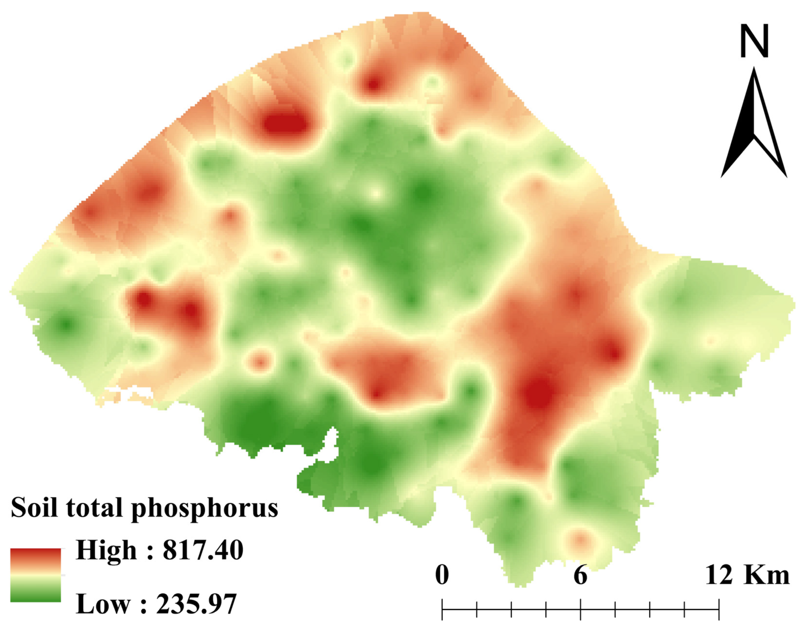
3.2. Characterization of Spatial Variability in Soil Total Phosphorus

Moran’s index results show that soil total phosphorus in the study area exhibits significant positive spatial autocorrelation (Moran’s I = 0.21, p < 0.01), and its spatial distribution displays clear clustering characteristics (Table S3). Additionally, we explored spatial heterogeneity of soil total phosphorus in the study area using GS+ 9.0. The model fitting results show that the semivariogram of soil total phosphorus conforms to the exponential model (R² = 0.894, RSS = 2.972 × 10⁻⁵). The nugget effect is 71.5%, and the range is 4200 m, further verifying the significant spatial clustering of soil total phosphorus in the study area (Table S4). The spatial distribution of soil total phosphorus was visualized using the ordinary kriging method based on the optimal semivariance model. The interpolation results show that soil total phosphorus in the study area is distributed in a patchy pattern, with obvious spatial heterogeneity, which aligns well with the topographic features of the study area (Figure 3). High-value areas were found in the cultivated areas distributed along the river, while low-value areas were mainly distributed in forest areas in the southeastern and central areas.

3.3. Analysis of Factors Influencing the Spatial Distribution of Soil Total Phosphorus

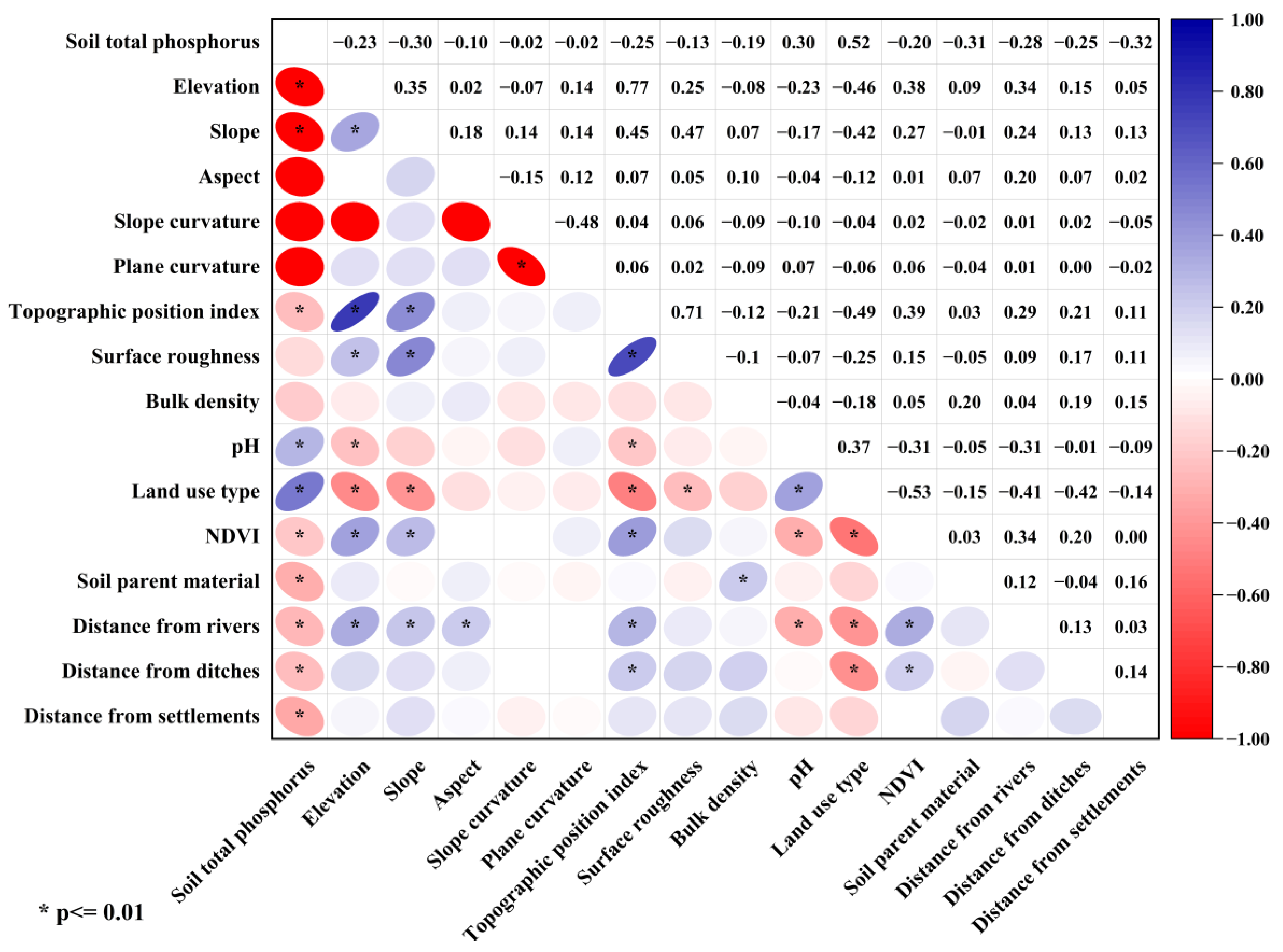
3.3.1. Pearson Correlation Analysis

Pearson’s correlation analysis (Figure 4) revealed that soil total phosphorus in the study area was highly significantly correlated (p < 0.01) with elevation, slope, TPI, soil pH, land use types, NDVI, soil parent material, and distance from rivers, settlements, and ditches. Among these, soil pH and land use types were positively correlated, while the others showed negative correlations. In terms of the correlation coefficients, the correlation coefficient between soil total phosphorus and land use types was 0.52, indicating a relatively strong positive correlation. The correlation between soil total phosphorus and the distance from settlements was −0.32, showing a negative correlation.

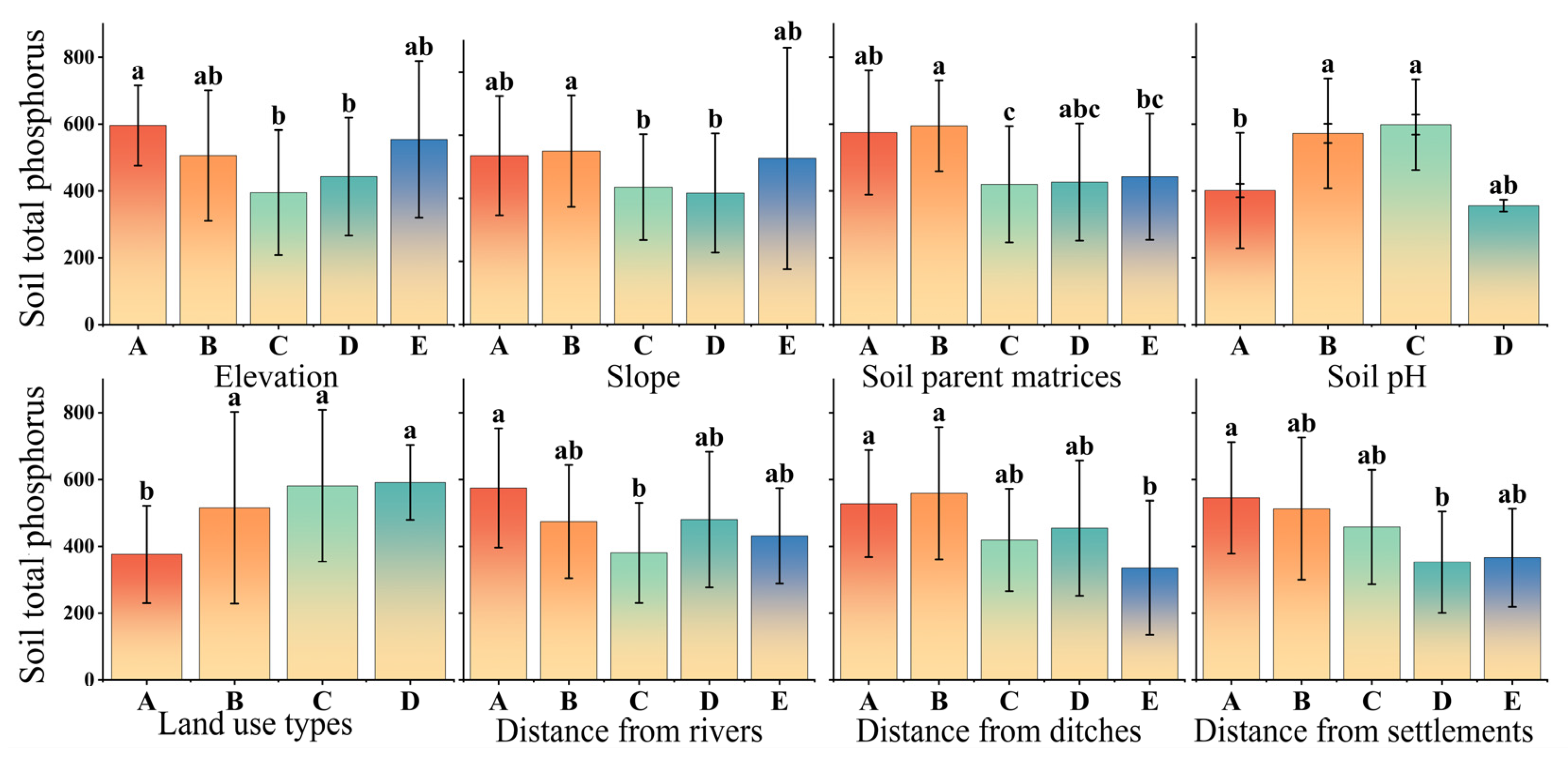
3.3.2. One-Way Analysis of Variance

In the study area, significant differences in the soil total phosphorus content were observed across various factors (Figure 5). Firstly, at different elevations, it decreased with increasing altitude below 28 m while it increased above 28 m. Secondly, under different slope classifications, the highest content was at 0–2° slope gradient and the lowest at ≥10°, thus showing a decrease with increased slope gradient. Thirdly, among different soil parent materials, river and lake sediments had the highest content, and red sandstone weathered materials had the lowest, and they were ranked as river and lake sediments > quaternary red clay > purple rock weathered materials > quartz sandstone weathered materials > red sandstone weathered materials. Fourthly, regarding different soil pH levels, the highest content was with soil pH < 4.5 and the lowest with soil pH > 6.5, with the content decreasing as the soil pH decreased. Fifthly, for different land use types, paddy fields had the highest content and forestland the lowest, following the order of paddy fields > dry land > orchard land > forest land. Finally, soil total phosphorus content exhibits a decreasing trend as the distance from rivers, ditches, and settlements increases. The maximum average content is observed at a distance ranging from 540 to 1240 m from the rivers, within a distance of less than 55 m from the ditches, and a distance of less than 110 m from the settlement, respectively.

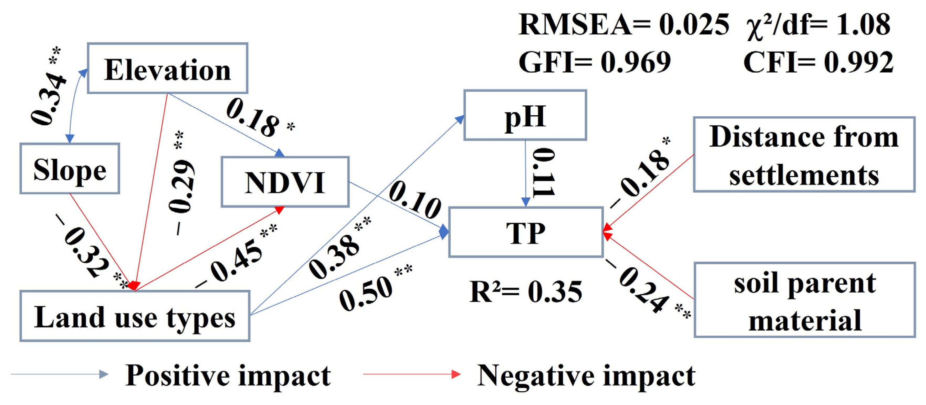
3.3.3. Structural Equation Modeling Analysis

In this study, considering the significance of the factors and their total effects, the three factors of TPI, distance from the rivers and distance from the ditches, and their corresponding paths were eliminated to construct the optimal SEM (Figure 6). The model results indicate that elevation indirectly affects soil total phosphorus through NDVI and land use types. Slope influences soil total phosphorus via land use types. Land use types indirectly affect soil total phosphorus through NDVI and soil pH. Elevation and slope interact with each other and have indirect effects on soil total phosphorus through land use types and NDVI. NDVI, land use types, soil pH, soil parent materials, and the distance from settlements have direct effects on soil total phosphorus. According to

Table 2. Total, direct, and indirect effects of factors influencing soil total phosphorus.

Influences	Total Effect	Direct Effect	Indirect Effect
Soil parent material	−0.240	−0.240	——
Elevation	−0.127	——	−0.127
Slope	−0.161	——	−0.161
soil pH	0.114	0.114	——
Land use types	0.499	0.505	0.005
NDVI	0.103	0.103	——
Distance to settlements	−0.178	−0.178	——

Note: —— denotes null value.

, land use types had the strongest total effect (0.499), while NDVI had the weakest (0.103). In terms of the absolute path coefficient of the direct effect, the direct effect of land use types is the highest (0.505), followed by that of soil parent materials (0.240). Based on the absolute value of indirect effects, slope exerted the strongest indirect influence (0.161), while land use types demonstrated the weakest (0.005), with these two values differing by approximately 32.2-fold.

4. Discussion

4.1. Main Factors and Mechanisms Affecting the Spatial Distribution of Soil Total Phosphorus

In this study, we found that land use types, distance from settlements, distance from rivers, distance from ditches, soil parent materials, elevation, slope, TPI, NDVI, and soil pH were significantly correlated with soil total phosphorus content in the study area, based on Pearson correlation analysis and ANOVA. For example, the soil total phosphorus content was highest in paddy fields, followed by dry land and orchard land, and lowest in forest land. Under different land use types, vegetation cover and anthropogenic disturbances affect the distribution of soil nutrients and physicochemical properties, resulting in substantial differences in soil total phosphorus content [37,38,39,40]. The high soil’s total phosphorus content may be attributed to the application of organic and chemical fertilizers during agricultural activities [41,42,43]. In addition, the total phosphorus content in forest soil was the lowest, because the forest land management mode was more extensive and the exogenous phosphorus input was less. Compared with forest, orchard soil had higher phosphorus levels due to increased fertilization application [44,45,46]. The aeration of dry land soils is better than that of paddy fields, which makes phosphorus more easily converted to phosphate, which may explain why dry land has lower total phosphorus content than paddy fields [47]. In addition, the negative correlation between distance from settlements and soil total phosphorus may reflect the influence of human activities. The closer to the residential areas, the more likely there will be more exogenous phosphorus input into the soil, thus affecting soil total phosphorus content [48,49,50]. For different soil parent materials, the soil total phosphorus content was the highest in the river and lake sediments and the lowest in the red sandstone weathered materials. The soil with river and lake sediments has a high content of soil total phosphorus because it has a strong ability to retain fertilizers and phosphate fertilizers are applied during farming [51]. The red sandstone weathered materials have a low total phosphorus content. This is because red sandstone typically has a low original phosphorus content and loose texture, resulting in poor fertilizer retention capacity [52,53]. However, soil total phosphorus content was negatively correlated with slope, which was inconsistent with the research findings on soil total phosphorus in hilly areas of southern China [54]. Zhang’s study [54] found that soil total phosphorus first increases with the increase in the slope and then slightly decreases as the slope further increases after reaching a peak. This may be related to the fact that the study area was on plains with little change in slope and does not have high soil total phosphorus loss. In terms of soil pH, the soil total phosphorus content was the highest in the range of 5.5–6.5. This is because in a weakly acidic environment, the balance between phosphorus fixation and dissolution reaches the optimal state, and the active soil microorganisms promote the mineralization of phosphorus [55,56]. Furthermore, the soil total phosphorus concentration increased with elevation, consistent with previous studies [57,58]. This is likely due to weaker weathering at high altitudes, which results in younger soil, reduced biomass consumption, and soil phosphorus accumulation [59,60].

The spatial distribution of soil total phosphorus in the study area was primarily affected by a combination of factors, and there were interactions among these factors. SEM was used to further analyze the pathways of influencing factors. First, land use types indirectly affect soil total phosphorus through NDVI and soil pH. Specifically, on one hand, different land use types can significantly change the vegetation cover, which is then reflected in NDVI [61,62,63]. For example, compared with natural forestlands, cultivated lands often show lower NDVI values due to frequent agricultural activities [64]. Vegetation cover directly affects the accumulation and decomposition of soil organic matter by regulating biogeochemical processes such as litter input and root exudates, thus changing the occurrence state of soil phosphorus [65,66]. On the other hand, different land use patterns can significantly change soil pH. As an example, farmlands with a long history of chemical fertilizer application typically have a lower soil pH than natural ecosystems [67]. The change in soil pH can significantly affect the chemical forms and availability of phosphorus, thereby influencing the spatial distribution of soil total phosphorus [68,69]. Second, elevation affects soil total phosphorus indirectly through slope, land use, and NDVI. As the elevation changes, the hydrothermal conditions change, which affects the growth and distribution of vegetation, and thus changes NDVI [70,71]. At the same time, elevation differences also affect the topography and geomorphology, resulting in different slopes. Steeper slopes are prone to soil erosion, which can carry away phosphorus elements in the soil, while gentle terrains are conducive to the accumulation of phosphorus [72,73]. Additionally, elevation changes can also affect human land use choices [74,75]. Different altitudes are suitable for different land use types, and different land use types, through their effects on vegetation and soil acidity and alkalinity mentioned above, indirectly act on the spatial distribution of soil total phosphorus. Third, slope indirectly affects soil total phosphorus through elevation and land use types. The slope is first closely related to elevation [76,77]. Different slopes often correspond to different elevation areas, thus affecting hydrothermal conditions and vegetation distribution [78,79]. It also affects the feasibility and mode of land use. In areas with larger slopes, forestry may be more suitable for development, while gentle areas are mostly used as cultivated lands [80]. Different land use types have different influencing methods and degrees on soil total phosphorus, so the slope indirectly acts on soil total phosphorus through elevation and land use types.

4.2. Recommendations for Controlling Soil Total Phosphorus in the Study Area

The accumulation of soil total phosphorus is an important aspect that causes eutrophication of water bodies and has gradually become a significant obstacle to sustainable development. Therefore, it is urgent to implement scientific and effective the soil total phosphorus management strategies. Previous studies have proposed some measures. For instance, Han et al. [81] proposed that the combination of optimized and reduced phosphorus application along with organic fertilizer could reduce loss from cultivated land. Nie et al. [82] found that precision fertilization and organic agriculture can reduce the loss of total soil phosphorus into water bodies. Chen et al. [83] found that terraced fields, vegetation buffer zones, and grass-planted streams reduced soil total phosphorus by using the Soil and Water Assessment Tool model. Considering the actual situation of the study area, we propose the following targeted measures to effectively control soil total phosphorus.

Because of the significant differences in the soil total phosphorus content in different land use types in the study area, it should be managed according to differentiation, such as precise fertilization in paddy fields and dry land, soil test and formula fertilization according to the actual soil total phosphorus content and crop demand, and strict control of phosphorus fertilizer application to avoid excessive application [84]. Since soil total phosphorus content decreases with the increase in distance from rivers and ditches, grassland filter strips can be set up between farmlands, forests, rivers, and ditches to use grassland vegetation and roots to intercept and purify phosphorus flowing into water bodies with surface runoff while regularly monitoring the phosphorus content in soil and water bodies and adjusting management strategies in a timely manner according to the monitoring data [85]. Finally, it is necessary to strengthen publicity and education for residents and farmers to enhance their awareness of soil protection and phosphorus management, prompting them to adopt environmentally friendly land management methods.

5. Conclusions

In this study, we comprehensively applied classical statistics, geostatistics, and SEM to systematically analyze the spatial distribution characteristics of soil total phosphorus and its influencing factors in the Haihunjiang River Basin. The results showed that the soil total phosphorus content in the study area exhibits a moderate level of spatial variation (CV = 37.76%) and significant spatial autocorrelation (Moran’s I = 0.208, p < 0.01). The spatial distribution of soil total phosphorus was the result of the interaction among various factors, such as land use types, soil parent materials, soil pH, elevation, slope, and distance to settlements, rivers, and ditches. The SEM revealed the pathways through which different influencing factors affect soil total phosphorus. According to the path coefficients, it was found that land use types and soil parent material were the leading factors for the spatial heterogeneity of soil total phosphorus. Our results provide a scientific basis for the prevention and control of non-point source phosphorus pollution in similar study areas. It is recommended to optimize agricultural land use patterns, strengthen phosphorus interception measures in lakeside areas, and formulate differential ecological restoration strategies in combination with topographic characteristics to achieve efficient soil phosphorus management and effectively mitigate the risk of water eutrophication.

References

1. Malhotra, H.; Vandana Sharma, S.; Pandey, R. Phosphorus Nutrition: Plant Growth in Response to Deficiency and Excess. In Plant Nutrients and Abiotic Stress Tolerance; Springer: Cham, Switzerland, 2018; pp. 171–190. [Google Scholar]
2. Yanardağ, A.B. Damage to Soil and Environment Caused by Excessive Fertilizer Use. In Agriculture, Forestry and Aquaculture Sciences; Serüven Publishing: Ankara, Turkey, 2024; p. 203. [Google Scholar]
3. Chen, M.; Li, Y.; Wang, C.; Walter, M.T.; Huang, L. Modelling rainfall-induced phosphorus loss with eroded clay and surface runoff. Hydrol. Process. 2023, 37, e14817. [Google Scholar] [CrossRef]
4. Han, J.; Xin, Z.; Han, F.; Xu, B.; Wang, L.; Zhang, C.; Zheng, Y. Source contribution analysis of nutrient pollution in a P-rich watershed: Implications for integrated water quality management. Environ. Pollut. 2021, 279, 116885. [Google Scholar] [CrossRef]
5. Foy, R.; Withers, P. The contribution of agricultural phosphorus to eutrophication. Proc. Fertil. Soc. 1995, 365, 1–32. [Google Scholar]
6. Liu, Z.-P.; Shao, M.-A.; Wang, Y.-Q. Spatial patterns of soil total nitrogen and soil total phosphorus across the entire Loess Plateau region of China. Geoderma 2013, 197, 67–78. [Google Scholar] [CrossRef]
7. Roger, A.; Libohova, Z.; Rossier, N.; Joost, S.; Maltas, A.; Frossard, E.; Sinaj, S. Spatial variability of soil phosphorus in the Fribourg canton, Switzerland. Geoderma 2014, 217, 26–36. [Google Scholar] [CrossRef]
8. Wang, J.; Ouyang, J.; Zhang, M. Spatial distribution characteristics of soil and vegetation in a reclaimed area in an opencast coalmine. Catena 2020, 195, 104773. [Google Scholar] [CrossRef]
9. Thuy, P.T.P.; Hoa, N.M.; Dick, W.A. Reducing phosphorus fertilizer input in high phosphorus soils for sustainable agriculture in the Mekong Delta, Vietnam. Agriculture 2020, 10, 87. [Google Scholar] [CrossRef]
10. He, X.; Augusto, L.; Goll, D.S.; Ringeval, B.; Wang, Y.; Helfenstein, J.; Huang, Y.; Yu, K.; Wang, Z.; Yang, Y.J.C.G. Global patterns and drivers of soil total phosphorus concentration. Earth Syst. Sci. Data Discuss 2021, 13, 5831–5846. [Google Scholar] [CrossRef]
11. Rubæk, G.H.; Kristensen, K.; Olesen, S.E.; Østergaard, H.S.; Heckrath, G. Phosphorus accumulation and spatial distribution in agricultural soils in Denmark. Geoderma 2013, 209, 241–250. [Google Scholar] [CrossRef]
12. Li, C.; Zhang, Y.; Fang, H. Changes of Total Phosphorus in Topsoil and the Correlations with Agricultural Land-Use Change Across the Chengdu Plain During the Past 40 Years. Chin. J. Soil Sci. 2022, 53, 187–194. [Google Scholar] [CrossRef]
13. Zhu, J.; Wu, A.; Zhou, G. Spatial distribution patterns of soil total phosphorus influenced by climatic factors in China’s forest ecosystems. Sci. Rep. 2021, 11, 5357. [Google Scholar] [CrossRef]
14. Han, Y.; Guo, X.; Jiang, Y.; Xu, Z.; Li, Z. Environmental factors influencing spatial variability of soil total phosphorus content in a small watershed in Poyang Lake Plain under different levels of soil erosion. Catena 2020, 187, 104357. [Google Scholar] [CrossRef]
15. Wang, R.; Zou, R.; Liu, J.; Liu, L.; Hu, Y. Spatial distribution of soil nutrients in farmland in a hilly region of the pearl river delta in China based on geostatistics and the inverse distance weighting method. Agriculture 2021, 11, 50. [Google Scholar] [CrossRef]
16. Biswas, A.; Biswas, A. Geostatistics in soil science: A comprehensive review on past, present and future perspectives. J. Indian Soc. Soil Sci. 2024, 72, 1–22. [Google Scholar] [CrossRef]
17. Gao, L.; Zhang, D.; Long, H.; Chen, X.; Lin, C.; Zhou, T. Interaction mechanism of climate, vegetation and soil factors on soil organic carbon at different soil depths in Ningxia. Acta Ecol. Sin. 2023, 43, 10081–10091. [Google Scholar] [CrossRef]
18. Yu, T.; Qian, H.; Zhou, Y.; Yang, M. Spatial distribution characteristics and influencing factors of soil nitrogen in damaged wetland in double-returned area of Poyang Lake. Acta Agric. Univ. Jiangxiensis 2024, 46, 530–542. [Google Scholar] [CrossRef]
19. Li, B.; Yang, G.; Wan, R.; Lai, X.; Wagner, P.D. Impacts of hydrological alteration on ecosystem services changes of a large river-connected lake (Poyang Lake), China. J. Environ. Manag. 2022, 310, 114750. [Google Scholar] [CrossRef]
20. Li, B.; Yang, G.; Wan, R. Multidecadal water quality deterioration in the largest freshwater lake in China (Poyang Lake): Implications on eutrophication management. Environ. Pollut. 2020, 260, 114033. [Google Scholar] [CrossRef]
21. Wu, Y.; Wang, H.; Deng, Y.; Li, X.; Xu, H. Evaluation and driving characteristics of water nutrients in Poyang lack based on TLI method. Environ. Eng. 2024, 42, 10–17. [Google Scholar] [CrossRef]
22. Shao, X. Regulations of Jiangxi Province on the Prevention and Control of Total Phosphorus Pollution in the Poyang Lake Basin. 30 November 2023. Available online: https://jxrd.jxnews.com.cn/system/2023/11/30/020317181.shtml (accessed on 18 February 2024).
23. Zhou, Y.; Zhao, X.; Guo, X. Influence Factors Analysis of Soil Trace Elements in Xunwu County Based on the Geographical Detector. J. Nucl. Agric. Sci. 2021, 35, 1420–1432. [Google Scholar] [CrossRef]
24. Balasubramanian, A. Digital Elevation Model (DEM) in GIS; University of Mysore: Mysore, India, 2017. [Google Scholar]
25. Borana, S.; Yadav, S. tpi-Based Vegetation Changes and Seasonal Variation in Semi Arid Region. In Proceedings of the ESRI India Conference-2018, Kolkata, India, 6 September 2018. [Google Scholar]
26. Jiang, Y.; Rao, L.; Guo, X. Spatial Variability of Farmland Soil Nitrogen of Jiangxi Province and Its Influencing Factors. Resour. Environ. Yangtze Basin 2018, 27, 70–79. [Google Scholar] [CrossRef]
27. Nielsen, D.R.; Bouma, J. Soil Spatial Variability: Proceedings of a Workshop of the ISSS and the SSSA, Las Vegas, USA/Pdc296; Center Agricultural Pub and Document, Pudoc Wageningen: Wageningen, The Netherlands, 1985. [Google Scholar]
28. Xu, Y.; Sun, H.; Ji, X. Spatial-temporal evolution and driving forces of rainfall erosivity in a climatic transitional zone: A case in Huaihe River Basin, eastern China. Catena 2021, 198, 104993. [Google Scholar] [CrossRef]
29. Zhang, C.; Lu, L.; Yang, H.; Huang, F. Spatial variation analysis of soil organic matter in karst area. Carsologica Sin. 2022, 41, 228–239. [Google Scholar]
30. Wang, H.; Zhu, Y.; Wang, J.; Han, H.; Niu, J.; Chen, X. Modeling of spatial pattern and influencing factors of cultivated land quality in Henan Province based on spatial big data. PLoS ONE 2022, 17, e0265613. [Google Scholar] [CrossRef]
31. Cambardella, C.A.; Moorman, T.B.; Novak, J.; Parkin, T.; Karlen, D.; Turco, R.; Konopka, A. Field-scale variability of soil properties in central Iowa soils. Soil Sci. Soc. Am. J. 1994, 58, 1501–1511. [Google Scholar] [CrossRef]
32. Li, Y.; Zhong, B.; Xu, X.; Liang, Z. Application of a semivariogram based on a deep neural network to Ordinary Kriging interpolation of elevation data. PLoS ONE 2022, 17, e0266942. [Google Scholar] [CrossRef]
33. Lu, X.; Yang, Q.; Wang, H.; Zhu, Y. A global meta-analysis of the correlation between soil physicochemical properties and lead bioaccessibility. J. Hazard. Mater. 2023, 453, 131440. [Google Scholar] [CrossRef] [PubMed]
34. Zhu, P.; Zhang, G.; Wang, C.; Chen, S.; Wan, Y. Variation in soil infiltration properties under different land use/cover in the black soil region of Northeast China. Int. Soil Water Conserv. Res. 2024, 12, 379–387. [Google Scholar] [CrossRef]
35. Yuan, K.; Deng, L. Equivalence of Partial-Least-Squares SEM and the Methods of Factor-Score Regression. Struct. Equ. Model. Multidiscip. J. 2021, 28, 557–571. [Google Scholar] [CrossRef]
36. Hu, Y.; Xiang, D.; Veresoglou, S.D.; Chen, F.; Chen, Y.; Hao, Z.; Zhang, X.; Baodong, C. Soil organic carbon and soil structure are driving microbial abundance and community composition across the arid and semi-arid grasslands in northern China. Soil Biol. Biochem. 2014, 77, 51–57. [Google Scholar] [CrossRef]
37. Huang, Y.; Ma, Y.; Hao, Y. Analysis of soil nutrient characteristics under typical land uses in north-eastern Ulan Buh Desert. Agric. Res. Arid. Areas 2019, 37, 123–129. [Google Scholar]
38. Li, X.; Liu, T.; Zhao, C.; Shao, M.; Cheng, J. Land use drives the spatial variability of soil phosphorus in the Hexi Corridor, China. Biogeochemistry 2021, 155, 59–75. [Google Scholar] [CrossRef]
39. Zhong, W.; Dong, Y.; Wang, S.; Ni, Z.; Wu, D.; Yang, Y.; Deng, Z. Evolution of watershed phosphorus buffering capacity and its response to land-use change in Poyang Lake basin, China. J. Clean. Prod. 2022, 365, 132606. [Google Scholar] [CrossRef]
40. Qiu, H.; Kuai, L.; Zhang, L. Characteristics of Acidity and Nutrient Changes in Red Soil After Conversion of Paddy Field to Dry Land and Vegetable Field. Sci. Agric. Sin. 2024, 57, 525–538. [Google Scholar] [CrossRef]
41. Liu, J.; Han, C.; Zhao, Y.; Yang, J.; Cade-Menun, B.J.; Hu, Y.; Li, J.; Liu, H.; Sui, P.; Chen, Y. The chemical nature of soil phosphorus in response to long-term fertilization practices: Implications for sustainable phosphorus management. J. Clean. Prod. 2020, 272, 123093. [Google Scholar] [CrossRef]
42. Hu, Q.; Wang, J.; Da, Y.; Sun, Y. The effects of plastic mulching and different fertilization on soil nutrients, yield and soil microbiome in maize field. Cereal Res. Commun. 2023, 51, 773–784. [Google Scholar] [CrossRef]
43. Yang, Y.; Zhang, H.; Qian, X.; Duan, J.; Wang, G. Excessive application of pig manure increases the risk of P loss in calcic cinnamon soil in China. Sci. Total Environ. 2017, 609, 102–108. [Google Scholar] [CrossRef]
44. Raiesi, T.; Moradi, B. Young navel orange rootstock improves phosphorus absorption from poorly soluble pools through rhizosphere processes. Rhizosphere 2021, 17, 100316. [Google Scholar] [CrossRef]
45. Yang, H.; Ji, L.; Long, L.; Ni, K.; Yang, X.; Ma, L.; Guo, S.; Ruan, J. Effect of Short-Term Phosphorus Supply on Rhizosphere Microbial Community of Tea Plants. Agronomy 2022, 12, 2405. [Google Scholar] [CrossRef]
46. Zou, Z.; Mi, W.; Li, X.; Hu, Q.; Zhang, L.; Zhang, L.; Fu, J.; Li, Z.; Han, W.; Yan, P. Biochar application method influences root growth of tea (Camellia sinensis L.) by altering soil biochemical properties. Sci. Hortic. 2023, 315, 111960. [Google Scholar] [CrossRef]
47. Leite, H.M.F.; Calonego, J.C.; de Moraes, M.F.; Mota, L.H.D.S.D.O.; da Silva, G.F.; do Nascimento, C.A.C. How a Long-Term Cover Crop Cultivation Impacts Soil Phosphorus Availability in a No-Tillage System? Plants 2024, 13, 2057. [Google Scholar] [CrossRef] [PubMed]
48. Smil, V. Phosphorus in the environment: Natural flows and human interferences. Annu. Rev. Energy Environ. 2000, 25, 53–88. [Google Scholar] [CrossRef]
49. Zhai, T.; Wang, J.; Fang, Y.; Qin, Y.; Huang, L.; Chen, Y. Assessing ecological risks caused by human activities in rapid urbanization coastal areas: Towards an integrated approach to determining key areas of terrestrial-oceanic ecosystems preservation and restoration. Sci. Total Environ. 2020, 708, 135153. [Google Scholar] [CrossRef] [PubMed]
50. Chen, C.; Zhang, X.; Webster, C. Spatially Explicit Impact of Land Use Changes in the Bay Area on Anthropogenic Phosphorus Emissions and Freshwater Eutrophication Potential. Environ. Sci. Technol. 2024, 58, 18701–18712. [Google Scholar] [CrossRef]
51. Xiong, J.; Lin, C.; Wu, Z.; Song, K.; Ma, R. Response of phosphorus in estuaries to soil erosion—A new insight into sediment phosphorus fractions and sources. Catena 2021, 207, 105665. [Google Scholar] [CrossRef]
52. Liu, D.; Cao, K.; Tang, Y.; Zhang, J.; Meng, X.; Ao, T.; Zhang, H. Study on weathering corrosion characteristics of red sandstone of ancient buildings under the perspective of non-destructive testing. J. Build. Eng. 2024, 85, 108520. [Google Scholar] [CrossRef]
53. Chen, C.; Zhao, B.; Zhang, L.; Huang, W. Mechanism of strength deterioration of red sandstone on reservoir bank slopes under the action of dry–wet cycles. Sci. Rep. 2023, 13, 20027. [Google Scholar] [CrossRef] [PubMed]
54. Zhang, J. Spatial and Temporal Changes of Soil Nutrients in Typical Red Soil Erosion Region of Southern China. Ph.D. Thesis, Fujian Normal University, Fuzhou, China, 2021. [Google Scholar]
55. Barrow, N. The effects of pH on phosphate uptake from the soil. Plant Soil 2017, 410, 401–410. [Google Scholar] [CrossRef]
56. Devau, N.; Le Cadre, E.; Hinsinger, P.; Jaillard, B.; Gérard, F. Soil pH controls the environmental availability of phosphorus: Experimental and mechanistic modelling approaches. Appl. Geochem. 2009, 24, 2163–2174. [Google Scholar] [CrossRef]
57. Huang, W.; Liu, C.; Liu, Y.; Huang, B.; Li, D.; Yuan, Z. Soil Ecological Stoichiometry and Its Influencing Factors at Different Elevations in Nanling Mountains. Ecol. Environ. Sci. 2023, 32, 80–89. [Google Scholar] [CrossRef]
58. Ma, Z. Spatial Heterogeneity of Soil Phosphorus and Its Influencing Factors in Guizhou Province. Ph.D. Thesis, Guizhou Normal University, Guiyang, China, 2023. [Google Scholar]
59. Von Blanckenburg, F.; Schuessler, J.; Bouchez, J.; Frings, P.; Uhlig, D.; Oelze, M.; Frick, D.A.; Hewawasam, T.; Dixon, J.; Norton, K. Rock weathering and nutrient cycling along an erodosequence. Am. J. Sci. 2021, 321, 1111–1163. [Google Scholar] [CrossRef]
60. Mou, X.; Wu, Y.; Niu, Z.; Jia, B.; Guan, Z.; Chen, J.; Li, H.; Cui, H.; Kuzyakov, Y.; Li, X. Soil phosphorus accumulation changes with decreasing temperature along a 2300 m altitude gradient. Agric. Ecosyst. Environ. 2020, 301, 107050. [Google Scholar] [CrossRef]
61. Hu, Y.; Raza, A.; Syed, N.R.; Acharki, S.; Ray, R.L.; Hussain, S.; Dehghanisanij, H.; Zubair, M.; Elbeltagi, A. Land use/land cover change detection and NDVI estimation in Pakistan’s Southern Punjab Province. Sustainability 2023, 15, 3572. [Google Scholar] [CrossRef]
62. Olexa, E.M.; Lawrence, R.L. Performance and effects of land cover type on synthetic surface reflectance data and NDVI estimates for assessment and monitoring of semi-arid rangeland. Int. J. Appl. Earth Obs. Geoinf. 2014, 30, 30–41. [Google Scholar] [CrossRef]
63. Tasser, E.; Tappeiner, U. Impact of land use changes on mountain vegetation. Appl. Veg. Sci. 2002, 5, 173–184. [Google Scholar] [CrossRef]
64. Wang, Z.; Xiao, P.; Zhang, P.; Sun, W.; Li, L.; Dong, F.; Hou, X.; Ma, L.; Jin, C. Mapping Spatio-Temporal Variations of Converting Farmland to Forest/Grassland on the Loess Plateau Using All Available Landsat Time-Series Images. In Proceedings of the IGARSS 2019–2019 IEEE International Geoscience and Remote Sensing Symposium, Yokohama, Japan, 28 July–2 August 2019. [Google Scholar]
65. Zhang, M.; O’Connor, P.J.; Zhang, J.; Ye, X. Linking soil nutrient cycling and microbial community with vegetation cover in riparian zone. Geoderma 2021, 384, 114801. [Google Scholar] [CrossRef]
66. Arruda, B.; Herrera, W.F.B.; Rojas-García, J.C.; Turner, C.; Pavinato, P.S. Cover crop species and mycorrhizal colonization on soil phosphorus dynamics. Rhizosphere 2021, 19, 100396. [Google Scholar] [CrossRef]
67. Luo, T.; Zhu, Y.; Lu, W.; Chen, L.; Min, T.; Li, J.; Wei, C. Acidic compost tea enhances phosphorus availability and cotton yield in calcareous soils by decreasing soil pH. Acta Agric. Scand. Sect. B—Soil Plant Sci. 2021, 71, 657–666. [Google Scholar] [CrossRef]
68. Wang, Y.; Zhang, W.; Müller, T.; Lakshmanan, P.; Liu, Y.; Liang, T.; Wang, L.; Yang, H.; Chen, X. Soil phosphorus availability and fractionation in response to different phosphorus sources in alkaline and acid soils: A short-term incubation study. Sci. Rep. 2023, 13, 5677. [Google Scholar] [CrossRef]
69. Chen, G.; Gan, L.; Wang, S.; Wan, G. Progess in geochemistry of phosphorus in soils. Earth Environ. 2001, 29, 78–81. [Google Scholar] [CrossRef]
70. Krakauer, N.Y.; Lakhankar, T.; Anadón, J.D. Mapping and attributing normalized difference vegetation index trends for Nepal. Remote Sens. 2017, 9, 986. [Google Scholar] [CrossRef]
71. Chen, W.; Xiao, A.; Braconnot, P.; Ciais, P.; Viovy, N.; Zhang, R. Mid-Holocene high-resolution temperature and precipitation gridded reconstructions over China: Implications for elevation-dependent temperature changes. Earth Planet. Sci. Lett. 2022, 593, 117656. [Google Scholar] [CrossRef]
72. Osman, K.T. Soils on Steep Slopes. In Management of Soil Problems; Springer: Cham, Switzerland, 2018; pp. 185–217. [Google Scholar]
73. Hua, D.; Li, J.; Xu, Y. Influence of Topographical Factors on Spatial Distribution Characteristics of Soil Nutrients in Qinba Mountain area. In Proceedings of the 2nd International Conference on Oil & Gas Engineering and Geological Sciences, IOP Conference Series: Earth and Environmental Science, Dalian, China, 4–5 July 2020. [Google Scholar]
74. Qasim, M.; Hubacek, K.; Termansen, M.; Fleskens, L. Modelling land use change across elevation gradients in district Swat, Pakistan. Reg. Environ. Change 2013, 13, 567–581. [Google Scholar] [CrossRef]
75. Birhanu, L.; Hailu, B.T.; Bekele, T.; Demissew, S. Land use/land cover change along elevation and slope gradient in highlands of Ethiopia. Remote Sens. Appl. Soc. Environ. 2019, 16, 100260. [Google Scholar] [CrossRef]
76. Evans, I.S.; Cox, N.J. Relations Between Land Surface Properties: Altitude, Slope and Curvature. In Process Modelling and Landform Evolution; Springer: Cham, Switzerland, 2005; pp. 13–45. [Google Scholar]
77. Warren, S.D.; Hohmann, M.G.; Auerswald, K.; Mitasova, H. An evaluation of methods to determine slope using digital elevation data. Catena 2004, 58, 215–233. [Google Scholar] [CrossRef]
78. He, J.; Zhao, W.; Li, A.; Wen, F.; Yu, D. The impact of the terrain effect on land surface temperature variation based on Landsat-8 observations in mountainous areas. Int. J. Remote Sens. 2019, 40, 1808–1827. [Google Scholar] [CrossRef]
79. Fan, B.; Tao, W.; Qin, G.; Hopkins, I.; Zhang, Y.; Wang, Q.; Lin, H.; Guo, L. Soil micro-climate variation in relation to slope aspect, position, and curvature in a forested catchment. Agric. For. Meteorol. 2020, 290, 107999. [Google Scholar] [CrossRef]
80. Tarolli, P.; Pijl, A.; Cucchiaro, S.; Wei, W. Slope instabilities in steep cultivation systems: Process classification and opportunities from remote sensing. Land Degrad. Dev. 2021, 32, 1368–1388. [Google Scholar] [CrossRef]
81. Han, X. Study on Dynamic Changes of Soil InorganicPhosphorus and Their Migration Characteristics of the Farmland in the Three Gorges Reservoir Area. Ph.D. Thesis, Southwest University, Chongqing, China, 2016. [Google Scholar]
82. Nie, J.; Haitao, F.; Xian, H. Coping Strategies for Eutrophication of Dianchi Lake. Low Carbon World 2023, 13, 13–15. [Google Scholar] [CrossRef]
83. Chen, J. Research on the Best Management Practices for Non-point Source Pollution in the Ashi River Basin Based on the SWAT Model. Ph.D. Thesis, Heilongjiang Universit, Harbin, China, 2023. [Google Scholar]
84. Liu, L.; Zheng, X.; Wei, X.; Kai, Z.; Xu, Y. Excessive application of chemical fertilizer and organophosphorus pesticides induced total phosphorus loss from planting causing surface water eutrophication. Sci. Rep. 2021, 11, 23015. [Google Scholar] [CrossRef]
85. Miao, K.; Dai, W.; Xie, Z.; Li, C.; Ye, C. Effect of Grass Buffer Strips on Nitrogen and Phosphorus Removal from Paddy Runoff and Its Optimum Widths. Agronomy 2023, 13, 2980. [Google Scholar] [CrossRef]
Figure 1. Overview of the study area and layout of sampling points.
Agriculture 15 01013 g001
Figure 2. Distributions of elevation (a), slope (b), aspect (c), slope curvature (d), plane curvature (e), topographic position index (f), surface roughness (g), normalized difference vegetation index (h), and soil parent material (i) in the study area.
Agriculture 15 01013 g002
Figure 3. Spatial distribution of soil total phosphorus by Kriging interpolation in the study area.
Agriculture 15 01013 g003
Figure 4. Pearson correlation analysis between soil total phosphorus and influencing factors (pH: soil pH; NDVI: normalized difference vegetation index). The values in the matrix are Pearson correlation coefficients, and * indicates the significance level (p ≤ 0.01)).
Agriculture 15 01013 g004
Figure 5. One-way analysis of variance showing the influence of different factors on soil total phosphorus. (In the figure, a and b denote significant intergroup differences at p < 0.05. A, B, C, D, and E represent different categories for various factors. Specific meanings are as follows: for elevation, A: 0–16 m, B: 16–27 m, C: 27–42 m, D: 42–62 m, and E: ≥62 m; for slope, A: 0–2°, B: 2–4°, C: 4–6°, D: 6–10°, and E: ≥10°; for soil pH, A: 3.70–4.50, B: 4.50–5.50, C: 5.50–6.50, and D: ≥6.50; for distance to rivers, A: 0–540 m, B: 540–1240 m, C: 1240–2000 m, D: 2000–3000 m, and E: ≥3000 m; for distance to ditches, A: 0–55 m, B: 55–140 m, C: 140–260 m, D: 260–450 m, and E: ≥450 m; for distance to settlements, A: 0–110 m, B: 110–230 m, C: 230–340 m, D: 340–550 m, and E: ≥550 m; for soil parent material, A is quaternary red clay, B is river and lake sediments, C is red sandstone weathered materials, D is quartz sandstone weathered materials, and E is purple rock weathered materials; for land use types, A is forest land, B is orchard land, C is dry land, and D is paddy fields).
Agriculture 15 01013 g005
Figure 6. Structural equation model results of the factors affecting soil total phosphorus in the study area. (TP—soil total phosphorus; NDVI—normalized difference vegetation index; pH—soil pH; * means p < 0.05, ** means p < 0.01).
Agriculture 15 01013 g006