Mitigating Catastrophic Forgetting in Pest Detection Through Adaptive Response Distillation

Abstract

Pest detection in agriculture faces the challenge of adapting to new pest species while preserving the ability to recognize previously learned ones. Traditional model fine-tuning approaches often result in catastrophic forgetting, where the acquisition of new classes significantly impairs the recognition performance of existing ones. Although knowledge distillation has been shown to effectively mitigate catastrophic forgetting, current research predominantly focuses on feature imitation, neglecting the extraction of potentially valuable information from responses.To address this issue, we introduce a response-based distillation method, called adaptive response distillation (ARD). ARD incorporates an adaptive response filtering strategy that dynamically adjusts the weights of classification and regression responses based on the significance of the information. This approach selectively filters and transfers valuable response data, ensuring efficient propagation of category and localization information. Our method effectively reduces catastrophic forgetting during incremental learning, enabling the student detector to maintain memory of old classes while assimilating new pest categories. Experimental evaluations on the large-scale IP102 pest dataset demonstrate that the proposed ARD method consistently outperforms existing state-of-the-art algorithms across various class-incremental learning scenarios, significantly narrowing the performance gap compared to fully trained models.

1. Introduction

Agriculture plays a crucial role in the global economy by providing food, raw materials, and employment opportunities for billions of people. With the global population continuously increasing and projected to reach 9.7 billion by 2050 [1], the agricultural sector faces immense pressure to meet the growing demand for food production. To address this challenge, precision agriculture emerges as a transformative solution, offering the potential to enhance agricultural productivity while reducing environmental impact. By leveraging advanced technologies such as satellite imagery, drones, sensors, and machine learning, precision agriculture enables farmers to monitor and manage crops with unprecedented precision at both macro and micro scales.

Satellite remote sensing, by providing large-scale, high-resolution imagery, assists farmers in monitoring crop health, soil moisture, and nutrient levels (nitrogen, phosphorus, and potassium), thereby optimizing agricultural management practices such as fertilization and irrigation [2,3]. Drones, on the other hand, can deliver higher-resolution images than satellite imagery and rapidly cover specific farmland areas, playing a vital role in pest monitoring and crop health assessment [4,5]. Sensor technologies, particularly those measuring soil moisture, temperature, and pH levels, enable farmers to monitor crop growing environments in real time. When combined with Internet of Things (IoT) technology, sensor data can be transmitted remotely and analyzed in real time, further enhancing the intelligence of irrigation and fertilization systems [6,7]. Additionally, machine learning and deep learning techniques, through processing and analyzing large-scale agricultural data, facilitate crop growth prediction, pest detection, and yield estimation, significantly improving the efficiency and accuracy of agricultural management [8,9].

Among these various applications, pest detection is a key task. Pests are significant factors contributing to agricultural losses, as insects and pathogens can spread rapidly on a large scale within a short period, leading to reduced crop yields or even complete crop failure. Therefore, the rapid and accurate detection and management of pests are crucial for agricultural production [10,11]. Object detection can automatically identify individual pests in images and accurately locate their positions within agricultural environments through image analysis. In recent years, with the rapid advancement of deep learning, algorithms such as convolutional neural networks (CNNs) have been successfully applied to pest detection, enabling improved recognition accuracy and robustness by automatically learning features from the data [12]. Through training on large annotated datasets, deep learning models can accurately recognize different pest species and perform real-time detection in complex agricultural settings [13].

In agriculture, object detection serves as a fundamental task and is widely applied in areas such as pest identification [14,15,16]. Ref. [17] provides a systematic review of the application of deep learning models (e.g., CNN, R-CNN, and their variants) in crop pest detection, highlighting that these methods outperform traditional approaches in terms of accuracy and efficiency. However, challenges persist in recognizing pests with limited sample sizes and diverse disease manifestations. Ref. [18] employed the YOLOv3 model for real-time detection of tomato leaf pests, with experimental results demonstrating high accuracy and rapid processing capabilities in both localization and classification, making it suitable for real-time monitoring in agricultural production. Ref. [19] enhanced the YOLO algorithm to improve the model’s ability to detect small targets and dense disease spots, with experiments showing a significant increase in detection accuracy under complex backgrounds. Ref. [20] combined transfer learning and data augmentation techniques with the Faster R-CNN model to achieve early identification of crop pests, particularly excelling in the initial stages of disease development. The multi-scale object detection method proposed in [21], through the introduction of a multi-scale feature fusion mechanism, further enhanced the accuracy of plant pest recognition, especially in handling disease spots of varying sizes. Additionally, refs. [22,23] utilized Faster R-CNN and YOLOv7, respectively, in conjunction with transfer learning techniques to achieve efficient detection of rice and maize pests, demonstrating the broad adaptability of deep learning models across different crops and environmental conditions.

However, the training of current deep learning models typically relies on the assumption of a static data distribution [24,25,26], with models often being deployed after a one-time training process. This static learning approach presents significant limitations in the dynamic environments characteristic of agriculture [27]. The types, population sizes, and distribution patterns of pests dynamically change over time, and the emergence of new pest categories necessitates models that can rapidly learn new classes while maintaining the ability to detect previously known pest categories. Nevertheless, directly fine-tuning the model with newly added data often leads to catastrophic forgetting [28,29], resulting in a substantial decline in the model’s performance in detecting old categories.

In the field of incremental learning, class incremental object detection (IOD) is one of the most challenging scenarios. Knowledge distillation (KD) [30], an effective technique for transferring knowledge from large-scale teacher models to smaller student models, has been widely applied to incremental object detection tasks in recent years. Existing work predominantly focuses on feature distillation [31,32,33], aiming to mitigate the forgetting of previously learned classes by preserving high-level feature information. For instance, ref. [32] proposed the first distillation framework for object detection by simply combining feature imitation and prediction imitation. Some studies [34,35,36,37] concentrate on selecting effective distillation regions to achieve more precise feature imitation, while other research [38,39,40] emphasizes optimizing the balance of imitation loss. Additionally, several methods [41,42,43,44] are dedicated to designing new teacher–student consistency functions, aiming to extract more consistency information or relax the stringent constraints of mean squared error (MSE) loss. In addition, ref. [32] performed distillation on all components of Faster R-CNN, including the backbone, proposals in RPN, and heads. Ref. [37] proposed a fine-grained feature imitation distillation method to allow the student model to mimic the high-level feature responses of the teacher model. Ref. [45] introduced a localization distillation method, applying knowledge distillation to the regression branch of the detector to help the student network resolve localization ambiguities. However, these approaches often overlook the critical information contained in the responses, including the probability distributions of classification predictions and the bounding box offsets of regression predictions. In contrast, response-based distillation methods can directly capture the inference process information of the teacher model, making them more suitable for incremental object detection tasks, particularly in dynamic pest detection environments.

This paper investigates a core issue in class incremental object detection tasks for pest detection: how to effectively learn responses from classification predictions and bounding boxes. In object detection, responses typically consist of classification logits and bounding box offsets. Due to the uncertainty in the number of objects in each new image, it is first necessary to validate all candidate responses to determine which are positive or negative samples, and to associate each object with its corresponding regression response. Additionally, as illustrated in Figure 1, studies have shown that only a subset of responses play a crucial role in preventing catastrophic forgetting. Therefore, it is essential to reasonably filter out an appropriate number of response nodes. To achieve this, we constrain key responses, enabling the student detector to learn and retain the teacher detector’s behavior patterns on old category targets, thereby ensuring the effectiveness of incremental pest object detection.

To address the challenges mentioned above, this paper proposes an adaptive response distillation (ARD) method, which effectively enhances the performance of incremental object detection by selectively learning the key response information from both classification and regression predictions. Specifically, the ARD method dynamically filters high-quality response nodes through statistical analysis, significantly reducing the interference of low-quality responses on the distillation process. Compared to traditional methods, ARD introduces incremental localization distillation in the regression branch, enabling the model to better handle the challenges of complex backgrounds and object ambiguity in pest detection. Moreover, the ARD method flexibly adjusts the filtering strategy based on data distribution characteristics, making it adaptable to different incremental task requirements.

The contributions of this paper can be summarized as follows,

(1) This paper is the first to explore response-based class-incremental object detection (CIOD) tasks on the IP102 dataset and investigates the effectiveness of applying response-based CIOD methods to pest detection, filling a gap in the current research.

(2) We thoroughly analyze the intrinsic differences between feature-based and response-based class-incremental object detection, and propose the ARD method, which dynamically filters high-quality response nodes through statistical analysis to optimize detection performance.

(3) The proposed ARD method significantly mitigates the problem of catastrophic forgetting in pest incremental detection tasks, achieving superior performance across multiple incremental learning scenarios, thus improving detection accuracy and robustness.

To the best of our knowledge, response-based knowledge distillation methods have not been explored for addressing continuous learning in agriculture-related tasks. Therefore, this paper leverages response-based knowledge distillation to support continuous learning for agricultural pest detection.

2. Materials and Methods

2.1. Datasets and Evaluation Metric

In this section, we simulate incremental learning scenarios using the publicly available large-scale pest dataset IP102 [46]. First, we compare incremental learning methods such as LwF [47], RILOD [48], SID [49], and ARD, and the experimental results validate the effectiveness of the proposed method. Subsequently, we conduct ablation studies to demonstrate the necessity of each component.

The IP102 dataset used in the experiments consists of 18,975 pest images, covering a total of 97 pest species, some of which are shown in Figure 2. We divided the dataset into training (70%), validation (15%), and testing (15%) sets. We adopt the standard COCO evaluation metrics, namely, $AP$, $A{P}_{50}$, and $A{P}_{75}$. In addition, we introduce two class-wise forgetting metrics—forgetting rate (FR) [50] and backward transfer (BWT) [51]—defined as follows:

For each old class c, let $A_c^{\mathrm{initial}}$ be its AP before any incremental steps, and $A_c^{\mathrm{final}}$ be its AP after all incremental steps. The class-wise FR is defined as:

$$F_c=A_c^{\mathrm{initial}}-A_c^{\mathrm{final}}$$

(1)

We then report the average FR over all old classes:

$$\overline{F}={\displaystyle \frac{1}{\left|C_{\mathrm{old}}\right|}}\sum _{c\in C_{\mathrm{old}}}{F}_c.$$

(2)

A lower $\overline{F}$ indicates better preservation of old-class knowledge. BWT is simply the negative of this quantity. BWT measures the average change in performance on old classes after incremental learning:

$$\mathrm{BWT}={\displaystyle \frac{1}{\left|C_{\mathrm{old}}\right|}}\sum _{c\in C_{\mathrm{old}}}\left(A_c^{\mathrm{final}}-A_c^{\mathrm{initial}}\right).$$

(3)

As $\overline{F}=-\mathrm{BWT}$ by definition, the two metrics differ only by sign. To maintain clarity and avoid redundancy, we propose to add only $\overline{F}$ which provides the same information as BWT while expressing performance loss directly.

Then, we converted the original dataset annotations, initially in Pascal-VOC format, into COCO annotation format. In the defined incremental learning scenarios, the parameter $a+b$ indicates that the initial stage begins with a base categories, and b new categories are added in each incremental step until all categories in the dataset are fully learned. However, at each incremental stage t, the model can only access the corresponding training set ${\mathcal{D}}^t$.

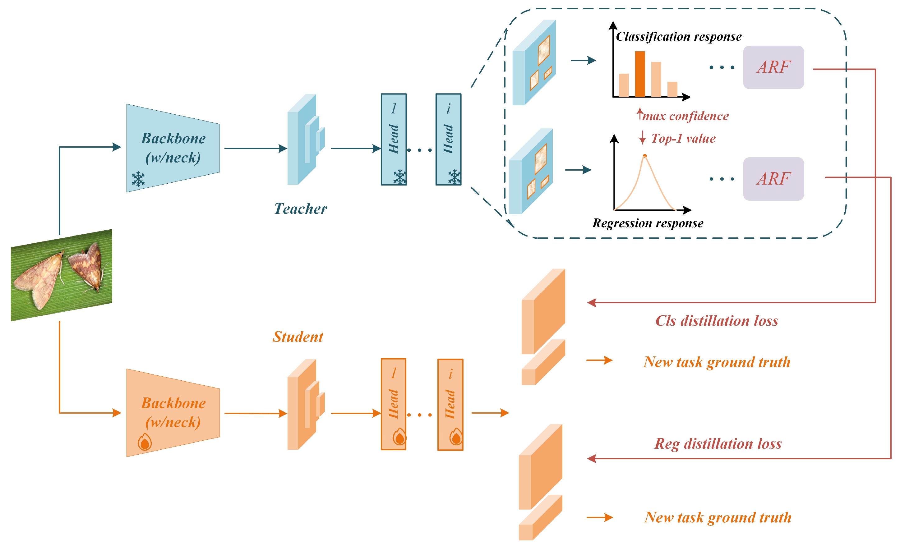
2.2. Overall Framework

The core objective of CIOD is to effectively transfer the knowledge learned by the existing network to the student detector. This knowledge encompasses features extracted from intermediate layers such as the backbone network or neck, as well as the soft targets generated by the detection heads. Unlike methods that rely on feature transfer, response-based strategies are capable of more comprehensively capturing the inference processes of the teacher detector [30,52]. Therefore, our approach incrementally filters and integrates knowledge from the responses of each detection head, thereby training a student object detector that is both high-performing and efficient.

The overall framework of the proposed method is illustrated in Figure 3. First, using the ARD method, we extract and learn the filtered responses from the classification and regression modules of the teacher detector. Next, we employ incremental localization distillation loss to enhance the student detector’s ability to extract localization information. Specifically, we introduce the adaptive response filtering (ARF) strategy, which selectively computes the distillation loss from the responses provided by the teacher detector, thereby obtaining more meaningful incremental responses. In summary, the total loss for training the student detector can be expressed as a weighted sum of the detection loss and the distillation loss, formulated as follows:

$$\mathcal{L}={\mathcal{L}}_{\mathit{cls}}({\mathcal{P}}_{gt},{\mathcal{P}}_S)+{\mathcal{L}}_{\mathit{reg}}({\mathcal{P}}_{gt},{\mathcal{P}}_S)+{\mathcal{L}}_{\mathit{ARD}}^{\mathit{cls}}({\mathcal{C}}_T,{\mathcal{C}}_S)+{\mathcal{L}}_{\mathit{ARD}}^{\mathit{reg}}({\mathcal{B}}_T,{\mathcal{B}}_S)$$

(4)

Here, the subscripts T and S represent the teacher model and the student model, respectively. ${\mathcal{L}}_{\mathit{cls}}({\mathcal{P}}_{gt},{\mathcal{P}}_S)$ and ${\mathcal{L}}_{\mathit{reg}}({\mathcal{P}}_{gt},{\mathcal{P}}_S)$ denote the classification loss and localization loss of the detector, which are calculated between the student’s predictions and the ground truth. The third loss term ${\mathcal{L}}_{\mathit{ARD}}^{\mathit{cls}}({\mathcal{C}}_T,{\mathcal{C}}_S)$ is the incremental classification distillation loss, and the fourth loss term ${\mathcal{L}}_{\mathit{ARD}}^{\mathit{reg}}({\mathcal{B}}_T,{\mathcal{B}}_S)$ is the incremental localization distillation loss for the regression branch. These are calculated between the student’s predictions and the teacher’s predictions. Both ${\mathcal{L}}_{\mathit{ARD}}^{\mathit{cls}}$ and ${\mathcal{L}}_{\mathit{ARD}}^{\mathit{reg}}$ are used for the outputs of the old classes.

2.3. Classification and Regression Head

Focal loss is used to solve the problem of class imbalance in object detection, where the foreground and background classes are unequally distributed. The formula is as follows:

$$FL\left(p\right)=-{(1-p_i)}^{\gamma }log\left(p_i\right),p_i=\left\{\begin{array}{cc}p,\hfill & y=1\hfill \\ 1-p,\hfill & y=0\hfill \end{array}\right.$$

(5)

where $y\in \{0,1\}$ represents the class label, and $p\in [0,1]$ is the predicted probability for class $y=1$. The FL includes a standard cross-entropy term $-log\left(p_t\right)$, and an adaptive term ${(1-p_t)}^{\gamma }$, which dynamically reduces the weight for easy samples, focusing on hard-to-detect samples.

In the GFLV1 [53], the quality focal loss (QFL) was proposed, which is used for supervision in the classification branch. It combines the location quality score and class score to represent the loss, reducing the constraints of one-hot class labels. The target value for each class is represented as a floating-point value $y\in [0,1]$. $y=0$ represents negative samples, and the location quality score is 0. $0<y\le 1$ represents positive samples, and y is the IoU score. Although this combined representation is used, the class imbalance problem still persists. Therefore, two parts of focal loss are extended.

The cross-entropy part $-log\left(p_t\right)$ is extended to its complete form:

$$-\left[\right(1-y)log(1-\sigma )+ylog(\sigma \left)\right]$$

(6)

The scaling multiplier ${(1-p_t)}^{\gamma }$ is generalized as the absolute distance between the predicted score $\sigma$ and the floating-point label y,

$${\left|y-\sigma \right|}^{\beta },(\beta \ge 0)$$

(7)

therefore, the expression for QFL is:

$$QFL\left(\sigma \right)=-{\left|y-\sigma \right|}^{\beta }\left[(1-y)log(1-\sigma )+ylog\left(\sigma \right)\right]$$

(8)

When $\sigma =y$, QFL is globally minimized. ${\left|y-\sigma \right|}^{\beta }$ is the adjustment coefficient. When the quality prediction $\sigma$ of a sample is not accurate and deviates from the label y, the adjustment coefficient increases, thus focusing more on difficult samples. When the quality prediction is accurate, $\sigma \to y$, this coefficient tends to 0, and the loss decreases. $\beta$ controls the reduction of the weight.

We use the relative offsets of the coordinate points to the four edges of the target box as the regression target. Traditional bounding box regression methods model the regression label y as a Dirac delta distribution $\delta (x-y)$, satisfying ${\int }_{-\infty }^{+\infty }\delta (x-y)dx=1$. This is typically implemented using fully connected layers. The Dirac delta distribution can be thought of as having infinite probability density at a single point, while the probability density at all other points is zero. Its integral form for recovery y is:

$$y={\int }_{-\infty }^{+\infty }\delta (x-y)xdx$$

(9)

However, in real-world scenarios, the object boundaries are not always well defined. Therefore, it is more reasonable to learn a distribution with a wider range. Given the label $y(y_0\le y\le y_n,n\in {\mathbb{N}}^{+})$, the predicted value $\widehat{y}(y_0\le \widehat{y}\le y_n)$ of the model is:

$$\widehat{y}={\int }_{-\infty }^{+\infty }P\left(x\right)xdx={\int }_{y_0}^{y_n}P\left(x\right)xdx$$

(10)

But CNNs use discrete representations, discretizing the value range $[y_0,y_n]$ into a set $\{y_0,y_1,\dots ,y_i,y_{i+1},\dots ,y_{n-1},y_n\}$, with intervals of $\mathrm{\Delta }$, i.e., uniformly sampling from the possible range $[y_0,y_n]$ of y. This transforms the problem from a regression problem into a multi-class classification problem. Given the discrete distribution properties ${\sum }_{i=1}^{n}P\left(y_i\right)=1$, the predicted regression value $\widehat{y}$ is represented as:

$$\widehat{y}=\sum _{i=0}^{n}P\left(y_i\right)·y_i$$

(11)

Using the softmax function, any discrete distribution can be easily implemented. $P\left(x\right)$ is implemented using $softmax$, with $P\left(y_i\right)$ denoted as ${\mathcal{S}}_i$. $\widehat{y}$ can be trained using SmoothL1, IoU loss, and GIoU loss. However, the value of $P\left(x\right)$ may have countless combinations to make the final integral result equal to y, which reduces learning efficiency. Therefore, distribution focal loss (DFL) is proposed, which increases the probability of $y_i$ and $y_{i+1}$ (the two points closest to y, $y_i\le y\le y_{i+1}$) to quickly focus the network on the points near label y. The bounding box learning only needs to focus on positive samples, avoiding concerns about class imbalance between positive and negative samples. Hence, the DFL form is as follows:

$$DFL({\mathcal{S}}_i,{\mathcal{S}}_{i+1})=-\left[(y_{i+1}-y)log\left({\mathcal{S}}_i\right)+(y-y_i)log\left({\mathcal{S}}_{i+1}\right)\right]$$

(12)

DFL works by increasing the probabilities of the two points on the left and right (${\mathcal{S}}_i$ and ${\mathcal{S}}_{i+1}$) of y, causing the network’s distribution to focus on the area near the label point. When DFL reaches the global minimum (i.e., ${\mathcal{S}}_i={\displaystyle \frac{y_{i+1}-y}{y_{i+1}-y_i}}$, ${\mathcal{S}}_{i+1}={\displaystyle \frac{y-y_i}{y_{i+1}-y_i}}$), it ensures that the predicted values $\widehat{y}$ approach the corresponding label y infinitely. QFL and DFL can be integrated into a unified form. Suppose a model predicts the probabilities of two variables $y_l,y_r(y_l<y_r)$ as $p_{y_i},p_{y_r},\left(p_{y_i}\ge 0,p_{y_r}\ge 0,p_{y_i}+p_{y_r}=1\right)$. Their linear combination prediction is $\widehat{y}=y_l{p}_{y_l}+y_r{p}_{y_r},(y_l\le \widehat{y}\le y_r)$. The corresponding continuous label y for predicting $\widehat{y}$ needs to satisfy $y_l\le y\le y_r$. The absolute distance ${\left|y-\sigma \right|}^{\beta },(\beta \ge 0)$ is used as the adjustment coefficient, and GFL can be written as:

$$GFL(p_{y_l},p_{y_r})=-{\left|y-(y_l{p}_{y_l}+y_r{p}_{y_r})\right|}^{\beta }((y_r-y)log\left(p_{y_l}\right)+(y-y_l)log\left(p_{y_r}\right))$$

(13)

In the following subsection, we apply the ARD method separately to the classification and regression heads of GFLV1. In the classification branch, we treat the classification scores predicted by the teacher as soft labels and directly utilize the QFL proposed in GFLV1 to bridge the teacher–student gap. In the regression branch, we represent the distribution of bounding box positions by predicting a vector, which contains more comprehensive information than the Dirac distribution represented by bounding boxes.

2.4. Application of ARD in the Classification Head

The soft predictions generated by the classification head of the teacher detector encapsulate recognition information for multiple categories. By learning these soft predictions, the student model is able to inherit the latent knowledge present in the teacher model, which is particularly intuitive in classification tasks. Let the teacher model be T, and apply the softmax function to convert the logits of ${\mathcal{C}}_T$ into probability distributions. The output probability distribution ${\mathcal{P}}_T$ is defined as:

$${\mathcal{P}}_T={\displaystyle \frac{e^{{\mathcal{C}}_T/t}}{{\sum }_{j=1}^m{e}^{{\mathcal{C}}_T/t}}}$$

(14)

The temperature factor t is used to adjust the smoothness of the probability distribution output by the softmax function. Similarly, let the student model be S, and the probability distribution output by the student model is defined as:

$${\mathcal{P}}_S={\displaystyle \frac{e^{{\mathcal{C}}_S/t}}{{\sum }_{j=1}^m{e}^{{\mathcal{C}}_S/t}}}$$

(15)

Previous studies often directly use all prediction results generated by the classification head and treat each response equally, that is,

$${\mathcal{L}}_{\mathit{cls}}=\sum _{i=1}^N{\mathcal{L}}_{\mathit{KL}}({\mathcal{P}}_T,{\mathcal{P}}_S)$$

(16)

where ${\mathcal{L}}_{\mathit{KL}}$ represents the KL-divergence between the teacher’s predictions ${\mathcal{P}}_T$ and the student’s predictions ${\mathcal{P}}_S$.

If not properly balanced, the responses of the background class may significantly outweigh those of the foreground classes, thereby hindering the retention of old knowledge. To address this issue, we selectively compute the distillation loss from the responses. Consequently, the incremental distillation loss for the classification head is defined as:

$${\mathcal{L}}_{\mathit{ARD}}^{\mathit{cls}}({\mathcal{C}}_T,{\mathcal{C}}_S)=\sum _{i=1}^n{\left({\mathcal{C}}_T^i-{\mathcal{C}}_S^i\right)}^2$$

(17)

Here, ${\mathcal{C}}_T^i$ represents one of the n category responses selected from the teacher detector based on the new data, and ${\mathcal{C}}_S^i$ corresponds to the response of the student detector for the same category. By extracting these selected responses, the student detector gradually inherits the existing knowledge of the teacher detector.

2.5. Application of ARD in the Regression Head

Previous studies have typically only used target bounding boxes with high classification confidence as the regression knowledge from the teacher detector, ignoring the role of localization information in the regression branch. By leveraging the general representation of bounding box distributions provided by the GFLV1 detector, each side of the bounding box can be converted into a probability distribution using the softmax function. Thus, the probability matrix for each bounding box is defined as follows:

$$\mathcal{B}=[p_t,p_b,p_l,p_r]\in {\mathbb{R}}^{n\times 4}$$

(18)

Therefore, we can extract the incremental localization information of the bounding box $\mathcal{B}$ from the teacher detector and transfer it to the student detector S using the KL-divergence loss as follows:

$${\mathcal{L}}_{\mathit{LD}}^j=\sum _{e\in \mathcal{B}}{\mathcal{L}}_{\mathit{KL}}^e\left({\mathcal{B}}_T^j,{\mathcal{B}}_S^j\right)$$

(19)

Finally, the incremental localization distillation loss for the regression head is defined as:

$${\mathcal{L}}_{\mathit{ARD}}^{\mathit{reg}}({\mathcal{B}}_T,{\mathcal{B}}_S)=\sum _{j=1}^J{\mathcal{L}}_{\mathit{LD}}^j$$

(20)

In this study, ${\mathcal{B}}_T^j$ represents the regression responses obtained by the teacher detector from the J selected bounding boxes based on the new data, while ${\mathcal{B}}_S^j$ denotes the corresponding regression responses from the student detector. Notably, the incremental localization distillation method provides additional localization information, further enhancing the performance of the student detector.

2.6. Adaptive Response Filtering

As shown in Figure 1, an excessive or insufficient number of responses can lead to a decline in model performance. Therefore, the careful selection of responses is crucial for preventing catastrophic forgetting. Existing selection methods often rely on sensitive hyperparameters, such as setting confidence thresholds or selecting top-k scores. These empirically driven strategies may result in the following issues: lower thresholds might overlook some old targets, while higher thresholds could introduce negative responses.

To address these challenges, we propose the ARF strategy. This strategy selects responses from the classification head and regression head separately, using them as distillation nodes.

2.6.1. Ensure Fairness Among Different Types of Responses

It is worth noting that in a normal distribution, approximately 16% and 2.5% of samples lie within the intervals $[\mu +\sigma ,+\infty ]$ and $[\mu +2\sigma ,+\infty ]$, respectively. In our context, the number of positive responses per image ranges between 100 and 1000. In contrast, strategies that involve selecting all responses or only the top-k responses can result in unfair treatment among different responses.

2.6.2. Statistical Analysis-Based ARF

In CIOD tasks, the responses generated by background objects can suppress the responses of foreground objects. Therefore, a higher $\mu$ value indicates a higher quality of the candidate response, while a lower $\mu$ value suggests lower quality. The ARF strategy can flexibly select a sufficient number of positive responses based on the statistical characteristics of each branch.

2.6.3. ARF in Classification Head

The classification branch selects responses from the classification head based on the statistical characteristics of confidence scores. First, the confidence score for each node is calculated. For each predicted value ${\mathcal{C}}_i^{\prime }$ in the classification scores ${\mathcal{C}}^{\prime }$, the confidence $G_{{\mathcal{C}}_i^{\prime }}$ for each predicted class is computed. The mean ${\mu }_{{\mathcal{C}}^{\prime }}$ and standard deviation ${\sigma }_{{\mathcal{C}}^{\prime }}$ of the confidence values $G_{{\mathcal{C}}_i^{\prime }}$ are then calculated. A threshold ${\tau }_{\mathcal{C}}^{\prime }$ is determined based on the mean and standard deviation, with a hyperparameter ${\alpha }_1$ used to adjust the sensitivity of the threshold, which is defined as ${\tau }_{{\mathcal{C}}^{\prime }}={\mu }_{{\mathcal{C}}^{\prime }}+{\alpha }_1{\sigma }_{{\mathcal{C}}^{\prime }}$. For each candidate class c in ${\mathcal{C}}^{\prime }$, if the confidence $G_{{\mathcal{C}}_i^{\prime }}$ is greater than or equal to the threshold ${\tau }_{\mathcal{C}}^{\prime }$, the candidate class c is added to the response set $\mathcal{C}$.

2.6.4. ARF in Regression Head

Similar to the classification branch, the responses of the regression head are also based on the statistical characteristics of confidence scores. For a specific bounding box in GFLV1, the distribution is often sharper, with the top-1 value being relatively larger. Therefore, the top-1 value is used as the confidence score for each bounding box. For each candidate box ${\mathcal{B}}_j^{\prime }$ in the bounding box predictions ${\mathcal{B}}^{\prime }$, the top-1 operation is applied to select the most likely bounding box $G_{{\mathcal{B}}_j^{\prime }}$, representing the box with the highest predicted probability. The mean ${\mu }_{{\mathcal{B}}^{\prime }}$ and standard deviation ${\sigma }_{{\mathcal{B}}^{\prime }}$ of the bounding box scores $G_{{\mathcal{B}}^{\prime }}$ are then calculated, and the threshold ${\tau }_{\mathcal{B}}^{\prime }$ is determined as ${\tau }_{{\mathcal{B}}^{\prime }}={\mu }_{{\mathcal{B}}^{\prime }}+{\alpha }_2{\sigma }_{{\mathcal{B}}^{\prime }}$, where ${\alpha }_2$ is a hyperparameter used to adjust the sensitivity of the threshold. Each candidate box b in ${\mathcal{B}}^{\prime }$ is evaluated, and those with a bounding box score $G_{{\mathcal{B}}^{\prime }}$ greater than or equal to ${\tau }_{\mathcal{B}}^{\prime }$ are added to the response set $\mathcal{B}$. Finally, non-maximum suppression (NMS) is applied to $\mathcal{B}$ to remove redundant and overlapping bounding boxes, ensuring that only the most relevant boxes are retained for further processing.

It is worth mentioning that all ARF uses a per-image, global-threshold approach: each image’s responses are independently aggregated across all classes to compute a single $\mu$ and $\sigma$, and a unified $\tau =\mu +\alpha \sigma$ is applied for selection, without any batch-level pooling or per-class thresholding.

3. Results

3.1. Implementation Details

The proposed ARD method is implemented within the Python 3.8-based MMDetection framework [54]. Both the teacher detector and the student detector are constructed based on the GFLV1 detector. The GFLV1 detector utilizes ResNet-50 as the backbone and FPN [55] as the neck. For fair comparison, all experiments are conducted using two Nvidia 4090 GPUs, with each GPU processing a mini-batch of 4 images. All experiments follow the default 1× training schedule, where one incremental step corresponds to 12 epochs. Unless otherwise specified, all hyperparameters are set to their default values as defined in the respective models for both training and testing. The default value of $\alpha$ is set to ${\alpha }_1={\alpha }_2=2$.

3.2. Single-Step Incremental Learning

We conduct a systematic comparison of key design aspects between existing incremental detection methods—such as LwF, RILOD, and SID—and our proposed ARD method. The results are summarized in

Table 1. Comparison of different design aspects of CIOD methods.

Dimensions	LwF	RILOD	SID	ARD (Ours)
Incremental Sample Handling	No replay of old samples	Replays old samples (replay buffer)	No replay of old samples	No replay of old samples
Old-Class Knowledge Retention	Classification logits	Sample replay + fine-tuning	Classification logits; Feature maps	Classification logits; Localization logits
Distillation Loss	KL	No distillation; relies on replay	KL; L2	L2; KL
Node/Region Selection	All classification responses	N/A	Main region (positives) + VLR (based on DIoU)	ARF: $\mu +\alpha \sigma$ threshold
Training Overhead	Low	High (replay cost grows with dataset size)	Medium (feature-hint + VLR computation)	Low (output-layer statistics + L2/KL distillation)

. In addition to LwF, RILOD, and SID, we also compare with a fine-tuning baseline method that does not employ any forgetting mitigation mechanisms, as well as joint training, which involves learning all classes simultaneously. The latter can be regarded as the upper limit for evaluating the ability of continual learning models to handle class-incremental challenges. The incremental scenario transitions from 49 + 48 to 85 + 12, with 12 classes added per step. As the number of base classes increases and the number of new classes decreases, we present the results of single-step incremental learning on IP102 in

Table 2. Comparison of performance ($AP$/$A{P}_{50}$/$A{P}_{75}$/$\overline{F}$, %) among incremental learning methods in sequential scenarios.

Scenarios (Classes)	Method	$\mathit{AP}$	${\mathit{AP}}_{50}$	${\mathit{AP}}_{75}$	$\overline{\mathit{F}}$
49 + 48	Fine-tuning	19.4	28.3	16.1	23.1
	LwF	15.5	28.6	13.9	27.0
	RILOD	26.3	43.5	28.8	16.2
	SID	32.8	47.9	31.4	9.7
	ARD	35.8	54.3	33.6	6.7
61 + 36	Fine-tuning	14.2	22.5	14.2	28.3
	LwF	10.1	15.8	9.6	32.4
	RILOD	25.5	42.3	28.6	17.0
	SID	29.2	46.0	30.3	13.3
	ARD	34.3	52.7	32.8	8.2
73 + 24	Fine-tuning	9.8	16.9	9.5	32.7
	LwF	7.3	12.4	8.4	35.2
	RILOD	24.6	40.4	27.8	17.9
	SID	30.4	43.2	28.9	12.1
	ARD	34.0	51.2	32.5	8.5
85 + 12	Fine-tuning	7.6	9.2	7.4	34.9
	LwF	8.9	13.3	8.7	33.6
	RILOD	23.7	38.4	24.8	18.8
	SID	29.4	41.1	29.1	13.1
	ARD	32.6	50.5	31.7	9.9
All classes	Joint Training	42.5	58.4	38.6

.

As shown in Table 2, the incremental learning results are presented for scenarios involving a) base classes and b) new classes. In the 49 + 48 incremental scenario, the $AP$ value for training on the full dataset is 42.5%. However, after fine-tuning the old detector with new data, the $AP$ value drops dramatically to 19.4%, indicating severe catastrophic forgetting as the model loses memory of the old classes during fine-tuning. In contrast, our method significantly outperforms the traditional fine-tuning strategy across all evaluation metrics, with improvements of 16.4%, 26.0%, and 17.5% in $AP$, $A{P}_{50}$, and $A{P}_{75}$, respectively. This demonstrates that our method effectively mitigates catastrophic forgetting. Notably, compared to the upper limit of class-incremental learning on the full dataset, the $AP$ is only 6.7% lower, showing that the student detector not only retains memory of the old classes well but also facilitates the learning of new classes. Furthermore, we report $\overline{F}$ to further analyze memory retention. In the 49 + 48 scenario, the fine-tuning baseline suffers a high forgetting rate of 23.1%, while our ARD method achieves the lowest forgetting rate of only 6.7%, indicating strong retention of prior knowledge.

As the number of base classes a increases and the number of new classes b decreases, the performance of traditional fine-tuning methods drops sharply, with catastrophic forgetting becoming increasingly severe. The $AP$ value declines from an initial 19.4% to 7.6%. In contrast, our method maintains a relatively high level of performance, mitigating catastrophic forgetting to some extent, as the $AP$ value only decreases from 35.8% to 32.6%, a reduction of just 3.2%. Correspondingly, ARD consistently outperforms all other methods in terms of $\overline{F}$. In the 85 + 12 setting, where forgetting is typically most severe, ARD maintains a relatively low forgetting rate of 9.9%, compared to 34.9% in fine-tuning. the forgetting rate only rises slightly from 6.7% to 9.9%, further validating the robustness of our method. This demonstrates that our method is highly robust in mitigating catastrophic forgetting, making it a promising solution for practical applications, particularly in dynamically changing environments where it can continuously enhance detector performance to meet real-world pest monitoring and management needs.

Moreover, in multiple incremental scenarios, our method consistently outperforms LwF, RILOD, and SID. While LwF performs well in traditional incremental classification tasks, it performs poorly in incremental detection tasks and, in some scenarios, even underperforms fine-tuning. This highlights its inability to address the complexity of object detection tasks. Under identical experimental settings, the results show that typical CIOD methods such as RILOD and SID are significantly less effective than our method. In four different incremental scenarios, our method achieves state-of-the-art performance, fully demonstrating its effectiveness in mitigating catastrophic forgetting.

Although the average AP value has improved, there is a possibility that the AP value of new pest classes increases while the AP value of old pest classes decreases. However, the larger increase in the AP value of new classes may mask the decline in the AP value of old classes. Despite this, the average AP value still increases, but this phenomenon is unreasonable because the decrease in the AP value of old classes indicates catastrophic forgetting, which contradicts the purpose of incremental learning. To avoid this controversy, this paper further analyzes the distribution of AP values for each class in the incremental method compared to joint training and catastrophic forgetting, and plots it as a histogram. From Figure 4, it can be seen that the AP value distribution for each class in the ARD method is similar to that of joint training, differing from the old class forgetting caused by catastrophic forgetting. This suggests that the ARD method is highly feasible in preserving the memory of old classes.

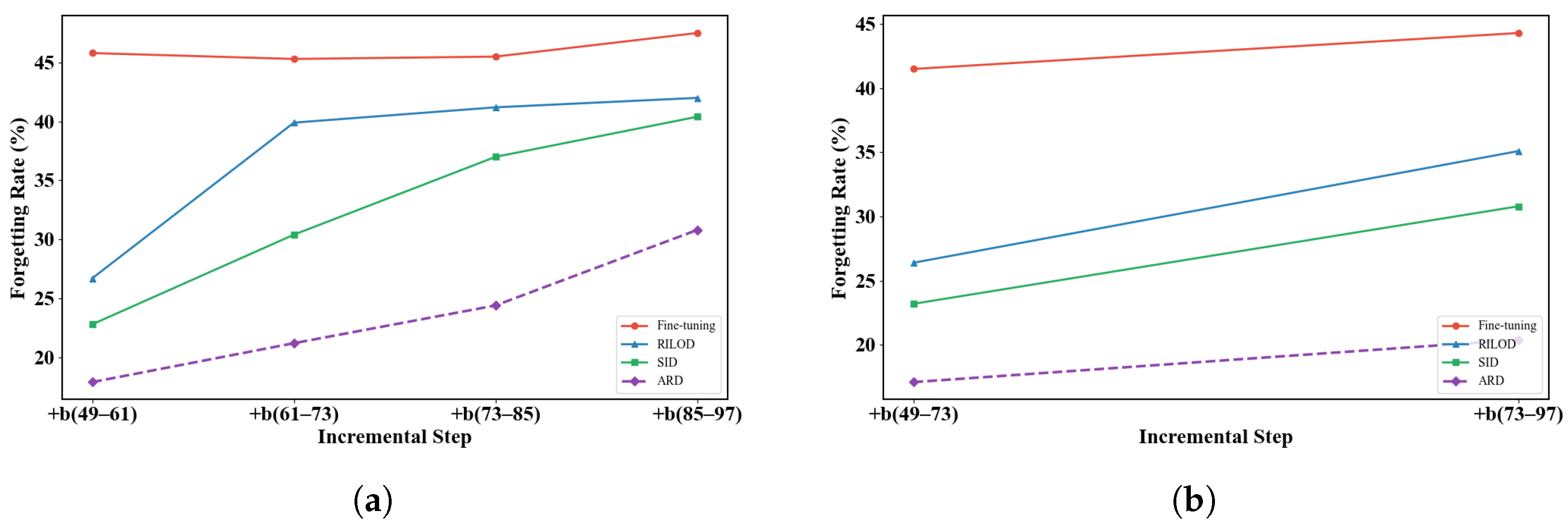
3.3. Multi-Step Incremental Learning

Multi-step incremental learning poses a more challenging objective for class-incremental learning, as it requires the model to retain knowledge from multiple tasks throughout consecutive learning steps.

Table 3. AP ($AP/A{P}_{50},\%$) performance among different methods in four-step incremental learning scenarios.

Method	a (1–49)	+b (49–61)	+b (61–73)	+b (73–85)	+b (85–97)	a (1–97)
Fine-tuning		7.8/9.7	8.3/10.3	8.1/10.5	6.1/8.4	42.5/58.4
RILOD	53.6/68.7	26.9/41.3	13.7/18.6	12.4/17.7	11.6/14.2
SID		30.8/48.1	23.2/34.3	16.6/25.6	13.2/23.8
ARD		35.7/54.2	32.4/47.6	29.2/40.8	22.8/32.5

(Four-Step) and

Table 4. AP ($AP/A{P}_{50},\%$) performance among different methods in two-step incremental learning scenarios.

Method	a (1–49)	+b (49–73)	+b (73–97)	a (1–97)
Fine-tuning		12.1/17.3	9.3/11.6	42.5/58.4
RILOD	53.6/68.7	27.2/44.9	18.5/26.0
SID		30.4/47.8	22.8/31.2
ARD		36.5/55.8	33.2/46.9

(Two-Step) present the experimental results under multi-step incremental learning scenarios. It is evident that our method significantly outperforms fine-tuning in both step settings. This is because as the detector learns new knowledge, such as new pest classes, this new knowledge interferes with previously learned knowledge, leading to catastrophic forgetting of the old pest classes. Our method effectively alleviates this issue by extracting meaningful responses at each incremental step, ensuring that key information is given focused attention. Compared to incremental algorithms such as RILOD and SID, our method also demonstrates clear advantages. Furthermore, in both multi-step scenarios, RILOD and SID exhibit significant $AP$ declines as new classes are continually added (from 26.9% to 11.6% and 30.8% to 13.2% for RILOD; 27.2% to 18.5% and 30.4% to 22.8% for SID). In contrast, our method shows a much slower and smaller decline in $AP$ (from 35.7% to 22.8% in Four-Step and from 36.5% to 33.2% in Two-Step), maintaining a relatively satisfactory performance level. The experimental results demonstrate the reliability of the ARD method in mitigating catastrophic forgetting during continual learning, making it a robust and effective solution.

To further analyze the behavior of different methods in preserving old knowledge, we plot the forgetting rate curves under both two-step and four-step incremental learning settings. These visualizations highlight the progression of forgetting across incremental stages and offer a clear comparison of the effectiveness of each method in mitigating catastrophic forgetting. The results in Figure 5 demonstrate that our proposed ARD method consistently achieves the lowest forgetting rate across all incremental steps. Compared to RILOD and SID, ARD not only starts from a lower forgetting level but also maintains a slower growth trend. In contrast, fine-tuning suffers from severe and persistent forgetting. These findings highlight the effectiveness and scalability of ARD in preserving old knowledge throughout progressive class-incremental learning.

We have conducted four sets of experiments to investigate the robustness of the proposed method with respect to the parameter $\alpha$. The method allows flexible selection of positive responses from both the classification and regression heads. In

Table 5. Comparison of incremental results (%) with different threshold combinations for 49 + 48 class incremental learning.

Threshold	$\mathit{AP}$	${\mathit{AP}}_{50}$	${\mathit{AP}}_{75}$	$\overline{\mathit{F}}$
${\alpha }_1=1,{\alpha }_2=1$	35.7	54.1	33.6	6.7
${\alpha }_1=1,{\alpha }_2=2$	35.5	54.6	33.9	6.7
${\alpha }_1=2,{\alpha }_2=1$	35.3	54.3	33.4	6.7
${\alpha }_1=2,{\alpha }_2=2$	35.8	54.3	33.6	6.7

, four different combinations of ${\alpha }_1,{\alpha }_2$ are selected for the training process. The experimental results show that the maximum performance difference is only 0.5%, and the forgetting rate even remains unchanged, indicating that the proposed ARD method is insensitive to changes in the parameter $\alpha$. Therefore, it can be concluded that the ARD method is almost independent of the parameter setting.

3.4. Ablation Study

We validate the effectiveness of each component of the proposed method in

Table 6. Ablation study (%) based on 49 classes + 48 classes.

Method	$\mathit{AP}$	${\mathit{AP}}_{50}$	${\mathit{AP}}_{75}$	$\overline{\mathit{F}}$
KD:cls + reg	30.7	47.3	29.2	11.5
KD:cls	24.8	35.7	24.9	18.9
KD:reg	15.7	22.1	16.2	26.0
ARD:cls	30.4	49.2	31.3	12.6
ARD:cls + reg	35.8	54.3	33.6	6.7

. In this table, “KD” represents the use of distillation loss without response selection; “ARD” introduces the response selection strategy. “KD:cls + reg” indicates that classification and regression responses are treated indiscriminately during incremental learning, while “KD:cls” and “KD:reg” handle only classification and regression responses, respectively. “ARD:cls” applies the ARF strategy for incremental distillation in the classification branch, and “ARD:cls + reg” applies the ARF strategy to both the classification and regression branches simultaneously. The experimental results show that the $AP$ for standard distillation of only the classification or regression branch is 24.8% and 15.7%, respectively. In contrast, combining the classification and regression responses yields an $AP$ of 30.7%. When we introduce the ARF strategy for distillation in the classification branch alone, the $AP$ improves to 30.4%. Furthermore, when the ARF strategy is applied to both the classification and regression branches, the $AP$ further increases to 35.8%. These results clearly demonstrate the significant advantages of the proposed method in mitigating catastrophic forgetting and enhancing pest detection performance. Overall, ARD consistently achieves the lowest forgetting rate among all configurations, particularly under the joint classification and regression setting. This highlights the effectiveness of ARF in preserving old knowledge during incremental learning. In contrast, standard KD methods suffer from significantly higher forgetting, especially when relying solely on regression branches.

3.5. Computational Cost Analysis

We provide a discussion of computational cost to facilitate a practical evaluation of ARD. All experiments were conducted on a workstation equipped with an Intel Intel 13th i9-13900K CPU, 256 GB RAM, and two NVIDIA 4090 GPUs (24 GB memory each). Training with ARD introduces approximately 4–6% additional time per epoch compared to the baseline KD:cls + reg method due to the ARF process. However, ARD does not introduce any additional computational overhead during inference. Moreover, as ARD only involves lightweight filtering based on logits during training, its additional memory consumption and computational complexity scale linearly with the number of samples, making it easily adaptable to common hardware setups. Therefore, the proposed method remains computationally efficient and practical for real-world deployment.

4. Discussion

The ARD method adopts a statistics-based ARF strategy to adaptively filter effective responses as distillation nodes, performing distillation on both the classification and regression branches. Specifically, it selects an appropriate number of response nodes from the teacher detector, which contain critical classification and regression soft predictions, and transfers these to the student detector. This process effectively mitigates catastrophic forgetting. Experimental results demonstrate that the ARD method not only enhances distillation performance but also achieves state-of-the-art detection accuracy.

In the future, we will explore the transferability of the ARD method across different agricultural scenarios and pest datasets to improve its generalization capabilities. Additionally, we aim to integrate multiple data sources (such as spectral information and environmental parameters) to further enhance the accuracy and robustness of pest detection.

5. Conclusions

To the best of our knowledge, this study is the first to explore continual object detection on a large-scale agricultural pest image dataset. For this purpose, we selected and curated a subset of data from the IP102 dataset specifically for pest detection, simulating incremental learning scenarios. Specifically, we simulated the learning process of the model for new pest classes using three settings: single-step incremental learning, four-step incremental learning, and two-step incremental learning. In each incremental step, the model was trained exclusively on the currently added classes. To address the common issue of catastrophic forgetting in incremental learning, we introduced the ARD method to mitigate the forgetting of old classes while enabling the continual learning of new classes. This approach enhances the overall performance of the pest detector by balancing the retention of previous knowledge and the acquisition of new knowledge.

References

1. Leong, D.P.; Teo, K.K.; Rangarajan, S.; Lopez-Jaramillo, P.; Avezum, A., Jr.; Orlandini, A. World Population Prospects 2019. World 2018, 73, 362. [Google Scholar]
2. Ennouri, K.; Kallel, A. Remote sensing: An advanced technique for crop condition assessment. Math. Probl. Eng. 2019, 2019, 9404565. [Google Scholar] [CrossRef]
3. Sishodia, R.P.; Ray, R.L.; Singh, S.K. Applications of remote sensing in precision agriculture: A review. Remote Sens. 2020, 12, 3136. [Google Scholar] [CrossRef]
4. Radoglou-Grammatikis, P.; Sarigiannidis, P.; Lagkas, T.; Moscholios, I. A compilation of UAV applications for precision agriculture. Comput. Netw. 2020, 172, 107148. [Google Scholar] [CrossRef]
5. Tsouros, D.C.; Bibi, S.; Sarigiannidis, P.G. A review on UAV-based applications for precision agriculture. Information 2019, 10, 349. [Google Scholar] [CrossRef]
6. Ahmad, N.; Hussain, A.; Ullah, I.; Zaidi, B.H. IOT based wireless sensor network for precision agriculture. In Proceedings of the 2019 7th International Electrical Engineering Congress (IEECON), Phetchaburi, Thailand, 7–9 March 2019; pp. 1–4. [Google Scholar]
7. Condran, S.; Bewong, M.; Islam, M.Z.; Maphosa, L.; Zheng, L. Machine learning in precision agriculture: A survey on trends, applications and evaluations over two decades. IEEE Access 2022, 10, 73786–73803. [Google Scholar] [CrossRef]
8. Kasinathan, T.; Singaraju, D.; Uyyala, S.R. Insect classification and detection in field crops using modern machine learning techniques. Inf. Process. Agric. 2021, 8, 446–457. [Google Scholar] [CrossRef]
9. Ang, K.L.M.; Seng, J.K.P. Big data and machine learning with hyperspectral information in agriculture. IEEE Access 2021, 9, 36699–36718. [Google Scholar] [CrossRef]
10. Butera, L.; Ferrante, A.; Jermini, M.; Prevostini, M.; Alippi, C. Precise agriculture: Effective deep learning strategies to detect pest insects. IEEE/CAA J. Autom. Sin. 2021, 9, 246–258. [Google Scholar] [CrossRef]
11. Saranya, T.; Deisy, C.; Sridevi, S.; Anbananthen, K.S.M. A comparative study of deep learning and Internet of Things for precision agriculture. Eng. Appl. Artif. Intell. 2023, 122, 106034. [Google Scholar] [CrossRef]
12. Lima, M.C.F.; de Almeida Leandro, M.E.D.; Valero, C.; Coronel, L.C.P.; Bazzo, C.O.G. Automatic detection and monitoring of insect pests—A review. Agriculture 2020, 10, 161. [Google Scholar] [CrossRef]
13. Kundur, N.C.; Mallikarjuna, P. Insect pest image detection and classification using deep learning. Int. J. Adv. Comput. Sci. Appl. 2022, 13, 411–421. [Google Scholar] [CrossRef]
14. Du, L.; Sun, Y.; Chen, S.; Feng, J.; Zhao, Y.; Yan, Z.; Zhang, X.; Bian, Y. A novel object detection model based on faster R-CNN for spodoptera frugiperda according to feeding trace of corn leaves. Agriculture 2022, 12, 248. [Google Scholar] [CrossRef]
15. Lippi, M.; Bonucci, N.; Carpio, R.F.; Contarini, M.; Speranza, S.; Gasparri, A. A yolo-based pest detection system for precision agriculture. In Proceedings of the 2021 29th Mediterranean Conference on Control and Automation (MED), Virtually, 22–25 June 2021; pp. 342–347. [Google Scholar]
16. Wang, R.; Liu, L.; Xie, C.; Yang, P.; Li, R.; Zhou, M. Agripest: A large-scale domain-specific benchmark dataset for practical agricultural pest detection in the wild. Sensors 2021, 21, 1601. [Google Scholar] [CrossRef]
17. Mittal, M.; Gupta, V.; Aamash, M.; Upadhyay, T. Machine learning for pest detection and infestation prediction: A comprehensive review. Wiley Interdiscip. Rev. Data Min. Knowl. Discov. 2024, 14, e1551. [Google Scholar] [CrossRef]
18. Huang, M.L.; Chuang, T.C.; Liao, Y.C. Application of transfer learning and image augmentation technology for tomato pest identification. Sustain. Comput. Inform. Syst. 2022, 33, 100646. [Google Scholar] [CrossRef]
19. Pang, H.; Zhang, Y.; Cai, W.; Li, B.; Song, R. A real-time object detection model for orchard pests based on improved YOLOv4 algorithm. Sci. Rep. 2022, 12, 13557. [Google Scholar] [CrossRef]
20. Arun, R.A.; Umamaheswari, S. Effective and efficient multi-crop pest detection based on deep learning object detection models. J. Intell. Fuzzy Syst. 2022, 43, 5185–5203. [Google Scholar] [CrossRef]
21. Tian, Y.; Wang, S.; Li, E.; Yang, G.; Liang, Z.; Tan, M. MD-YOLO: Multi-scale Dense YOLO for small target pest detection. Comput. Electron. Agric. 2023, 213, 108233. [Google Scholar] [CrossRef]
22. Khairunniza-Bejo, S.; Ibrahim, M.F.; Hanafi, M.; Jahari, M.; Ahmad Saad, F.S.; Mhd Bookeri, M.A. Automatic Paddy Planthopper Detection and Counting Using Faster R-CNN. Agriculture 2024, 14, 1567. [Google Scholar] [CrossRef]
23. Yang, S.; Xing, Z.; Wang, H.; Dong, X.; Gao, X.; Liu, Z.; Zhang, X.; Li, S.; Zhao, Y. Maize-YOLO: A new high-precision and real-time method for maize pest detection. Insects 2023, 14, 278. [Google Scholar] [CrossRef] [PubMed]
24. Albanese, A.; Nardello, M.; Brunelli, D. Automated pest detection with DNN on the edge for precision agriculture. IEEE J. Emerg. Sel. Top. Circuits Syst. 2021, 11, 458–467. [Google Scholar] [CrossRef]
25. Li, X.; Wang, W.; Hu, X.; Li, J.; Tang, J.; Yang, J. Generalized focal loss v2: Learning reliable localization quality estimation for dense object detection. In Proceedings of the IEEE/CVF Conference on Computer Vision and Pattern Recognition, Nashville, TN, USA, 20–25 June 2021; pp. 11632–11641. [Google Scholar]
26. Tian, Z.; Shen, C.; Chen, H.; He, T. Fcos: Fully convolutional one-stage object detection. In Proceedings of the IEEE/CVF International Conference on Computer Vision, Montreal, BC, Canada, 11–17 October 2021; pp. 9627–9636. [Google Scholar]
27. Lesort, T.; Lomonaco, V.; Stoian, A.; Maltoni, D.; Filliat, D.; Díaz-Rodríguez, N. Continual learning for robotics: Definition, framework, learning strategies, opportunities and challenges. Inf. Fusion 2020, 58, 52–68. [Google Scholar] [CrossRef]
28. Goodfellow, I.J.; Mirza, M.; Xiao, D.; Courville, A.; Bengio, Y. An empirical investigation of catastrophic forgetting in gradient-based neural networks. arXiv 2013, arXiv:1312.6211. [Google Scholar]
29. McCloskey, M.; Cohen, N.J. Catastrophic interference in connectionist networks: The sequential learning problem. Psychol. Learn. Motiv. 1989, 24, 109–165. [Google Scholar]
30. Hinton, G.; Vinyals, O.; Dean, J. Distilling the knowledge in a neural network. arXiv 2015, arXiv:1503.02531. [Google Scholar]
31. Chen, P.; Liu, S.; Zhao, H.; Jia, J. Distilling knowledge via knowledge review. In Proceedings of the IEEE/CVF Conference on Computer Vision and Pattern Recognition, Nashville, TN, USA, 20–25 June 2021; pp. 5008–5017. [Google Scholar]
32. Chen, G.; Choi, W.; Yu, X.; Han, T.; Chandraker, M. Learning efficient object detection models with knowledge distillation. In Proceedings of the Advances in Neural Information Processing Systems, Long Beach, CA, USA, 4–9 December 2017; Volume 30. [Google Scholar]
33. Sun, R.; Tang, F.; Zhang, X.; Xiong, H.; Tian, Q. Distilling object detectors with task adaptive regularization. arXiv 2020, arXiv:2006.13108. [Google Scholar]
34. Dai, X.; Jiang, Z.; Wu, Z.; Bao, Y.; Wang, Z.; Liu, S.; Zhou, E. General instance distillation for object detection. In Proceedings of the IEEE/CVF Conference on Computer Vision and Pattern Recognition, Nashville, TN, USA, 20–25 June 2021; pp. 7842–7851. [Google Scholar]
35. Jia, Z.; Sun, S.; Liu, G.; Liu, B. Mssd: Multi-scale self-distillation for object detection. Vis. Intell. 2024, 2, 8. [Google Scholar] [CrossRef]
36. Li, Q.; Jin, S.; Yan, J. Mimicking very efficient network for object detection. In Proceedings of the IEEE Conference on Computer Vision and Pattern Recognition, Honolulu, HI, USA, 21–26 July 2017; pp. 6356–6364. [Google Scholar]
37. Wang, T.; Yuan, L.; Zhang, X.; Feng, J. Distilling object detectors with fine-grained feature imitation. In Proceedings of the EEE/CVF Conference on Computer Vision and Pattern Recognition, Long Beach, CA, USA, 15–20 June 2019; pp. 4933–4942. [Google Scholar]
38. Guo, J.; Han, K.; Wang, Y.; Wu, H.; Chen, X.; Xu, C.; Xu, C. Distilling object detectors via decoupled features. In Proceedings of the IEEE/CVF Conference on Computer Vision and Pattern Recognition, Nashville, TN, USA, 20–25 June 2021; pp. 2154–2164. [Google Scholar]
39. Li, G.; Li, X.; Wang, Y.; Zhang, S.; Wu, Y.; Liang, D. Knowledge distillation for object detection via rank mimicking and prediction-guided feature imitation. AAAI Conf. Artif. Intell. 2022, 36, 1306–1313. [Google Scholar] [CrossRef]
40. Zhixing, D.; Zhang, R.; Chang, M.; Liu, S.; Chen, T.; Chen, Y. Distilling object detectors with feature richness. Adv. Neural Inf. Process. Syst. 2021, 34, 5213–5224. [Google Scholar]
41. Cao, W.; Zhang, Y.; Gao, J.; Cheng, A.; Cheng, K.; Cheng, J. Pkd: General distillation framework for object detectors via pearson correlation coefficient. Adv. Neural Inf. Process. Syst. 2022, 35, 15394–15406. [Google Scholar]
42. Yang, Z.; Li, Z.; Jiang, X.; Gong, Y.; Yuan, Z.; Zhao, D.; Yuan, C. Focal and global knowledge distillation for detectors. In Proceedings of the IEEE/CVF Conference on Computer Vision and Pattern Recognition, New Orleans, LA, USA, 18–24 June 2022; pp. 4643–4652. [Google Scholar]
43. Yao, L.; Pi, R.; Xu, H.; Zhang, W.; Li, Z.; Zhang, T. G-detkd: Towards general distillation framework for object detectors via contrastive and semantic-guided feature imitation. In Proceedings of the IEEE/CVF International Conference on Computer Vision, Montreal, BC, Canada, 11–17 October 2021; pp. 3591–3600. [Google Scholar]
44. Zhang, L.; Ma, K. Improve object detection with feature-based knowledge distillation: Towards accurate and efficient detectors. In Proceedings of the International Conference on Learning Representations, Addis Ababa, Ethiopia, 30 April 2020. [Google Scholar]
45. Zhengetal, Z. Localization distillation for object detection. IEEE Trans. Pattern Anal. Mach. Intell 2023, 45, 10070–10083. [Google Scholar]
46. Wu, X.; Zhan, C.; Lai, Y.K.; Cheng, M.M.; Yang, J. Ip102: A large-scale benchmark dataset for insect pest recognition. In Proceedings of the IEEE/CVF Conference on Computer Vision and Pattern Recognition, Long Beach, CA, USA, 15–20 June 2019; pp. 8787–8796. [Google Scholar]
47. Li, Z.; Hoiem, D. Learning without forgetting. IEEE Trans. Pattern Anal. Mach. Intell. 2017, 40, 2935–2947. [Google Scholar] [CrossRef] [PubMed]
48. Li, D.; Tasci, S.; Ghosh, S.; Zhu, J.; Zhang, J.; Heck, L. RILOD: Near real-time incremental learning for object detection at the edge. In Proceedings of the 4th ACM/IEEE Symposium on Edge Computing, Washington, DC, USA, 7–9 November 2019; pp. 113–126. [Google Scholar]
49. Peng, C.; Zhao, K.; Maksoud, S.; Li, M.; Lovell, B.C. Sid: Incremental learning for anchor-free object detection via selective and inter-related distillation. Comput. Vis. Image Underst. 2021, 210, 103229. [Google Scholar] [CrossRef]
50. Chaudhry, A.; Dokania, P.K.; Ajanthan, T.; Torr, P.H. Riemannian walk for incremental learning: Understanding forgetting and intransigence. In Proceedings of the European Conference on Computer Vision (ECCV), Munich, Germany, 8–14 September 2018; pp. 532–547. [Google Scholar]
51. Lopez-Paz, D.; Ranzato, M. Gradient episodic memory for continual learning. In Proceedings of the Advances in Neural Information Processing Systems, Long Beach, CA, USA, 4–9 December 2017; Volume 30. [Google Scholar]
52. Müller, R.; Kornblith, S.; Hinton, G.E. When does label smoothing help? In Proceedings of the Advances in Neural Information Processing Systems, Vancouver, BC, Canada, 8–14 December 2019; Volume 32.
53. Li, X.; Wang, W.; Wu, L.; Chen, S.; Hu, X.; Li, J.; Tang, J.; Yang, J. Generalized focal loss: Learning qualified and distributed bounding boxes for dense object detection. Adv. Neural Inf. Process. Syst. 2020, 33, 21002–21012. [Google Scholar]
54. Chen, K.; Wang, J.; Pang, J.; Cao, Y.; Xiong, Y.; Li, X.; Sun, S.; Feng, W.; Liu, Z.; Xu, J.; et al. MMDetection: Open mmlab detection toolbox and benchmark. arXiv 2019, arXiv:1906.07155. [Google Scholar]
55. Lin, T.Y.; Dollár, P.; Girshick, R.; He, K.; Hariharan, B.; Belongie, S. Feature pyramid networks for object detection. In Proceedings of the IEEE Conference on Computer Vision and Pattern Recognition, Honolulu, HI, USA, 21–26 July 2017; pp. 2117–2125. [Google Scholar]
Figure 1. AP (%) distribution across responses.
Agriculture 15 01006 g001
Figure 2. Examples of various pest species images for IP102 Pest Detection Dataset: (a) asiatic rice borer, (b) brown plant hopper, (c) paddy stem maggot, (d) rice gall midge, (e) rice leaf roller, (f) rice stemfly, (g) rice water weevil, (h) wheat blossom midge, (i) large cutworm, (j) green bug, (k) red spider, (l) wireworm.
Agriculture 15 01006 g002
Figure 3. Overall framework of adaptive response distillation.
Agriculture 15 01006 g003
Figure 4. AP (%) for each class across different incremental learning methods. (a) Upper Bound. (b) Catastrophic Forgetting. (c) Adaptive Response Distillation.
Agriculture 15 01006 g004
Figure 5. Comparison of forgetting rates (%) across incremental learning steps. (a) Four-step. (b) Two-step.
Agriculture 15 01006 g005