A Track-Type Orchard Mower Automatic Line Switching Decision Model Based on Improved DeepLabV3+

Abstract

To achieve unmanned line switching operations for a track-type mower in orchards, an automatic line switching decision model based on machine vision has been designed. This model optimizes the structure of the DeepLabV3+ semantic segmentation model, using semantic segmentation data from five stages of the line switching process as the basis for generating navigation paths and adjusting the posture of the track-type mower. The improved model achieved an average accuracy of 91.84% in predicting connected areas of three types of headland environments: freespace, grassland, and leaf. The control system equipped with this model underwent automatic line switching tests for the track-type mower, achieving a success rate of 94% and an average passing time of 12.58 s. The experimental results demonstrate that the improved DeepLabV3+ model exhibits good performance, providing a method for designing automatic line switching control systems for track-type mowers in orchard environments.

1. Introduction

The track-type mower in orchards plays an increasingly important role in the management of modern dwarf rootstock dense planting orchards. Traditional weeding methods often rely on manual labor or non-automated machinery, which are inefficient and labor-intensive. Currently, track-type mowers in orchards have achieved significant improvements in management efficiency through automated designs equipped with high-precision sensors for autonomous linear operations between rows. However, automatic line switching at the headland still requires manual operation.

Using radio technology to manually remote-control an orchard mower for the mowing task is economical and makes it easier to realize the line switching control of the mower, but the workload is large and the mowing task is restricted by the weather. Ultrasonic radar transmits and receives high-frequency sound waves and uses the principle of echolocation to detect the distance between the vehicle body and surrounding obstacles. Lidar transmits and receives infrared light waves and builds an environmental model in the form of point clouds. The two radars collect information on the surrounding environment, but they have difficulty classifying different kinds of objects in the environment. As a result, environmental information is missing during the line switching process, and the automatic line switching of the mower cannot be effectively controlled. GNSS technology can control the mower to move accurately, but it requires the locator to be positioned in advance to achieve automatic steering. When the number of operation lines is large, early positioning is more complex. Due to obstructions in the terrain and tree crowns, orchards distributed in hilly and mountainous areas will have weakened satellite signals, resulting in navigation deviation and an inability to switch the working lines automatically. Machine vision navigation is cost-effective, flexible in operation, and rich in information acquisition. This technology uses visual sensors to collect characteristic information about weeds, fruit trees, and exposed ground at the headland, allowing for precise identification and localization of weed boundaries in orchards. This provides a solution for the mower to autonomously plan its path and achieve automatic line switching. However, the actual environmental conditions at the headlands of apple orchards are complex; weed areas may be irregular and affected by obstacles such as lower branches of fruit trees, creating an unstructured environment that increases the difficulty of headland environment recognition. The challenges of path recognition in unstructured environments include complex path shapes, ambiguous boundaries, and susceptibility to changes in lighting conditions [1,2]. Therefore, accurately perceiving and reliably guiding the mower through the headland environment using machine vision technology to achieve automatic line switching remains challenging.

Researchers both domestically and internationally have conducted in-depth studies on path area recognition in unstructured environments. Xue J.L. et al. observed the environment by rotating to change the field of view (FOV) of the camera and used mathematical morphological operations to segment and describe crops. They planned paths based on the distribution characteristics of the crops, enabling agricultural robots to make automatic turns at the corners of corn fields [3]. Li Jingbin et al. studied navigation route and headland image detection algorithms for cotton-film mulching planters during field operations, quickly and accurately detecting navigation routes during cotton-film mulching operations and identifying the headland [4]. Liang Xihui et al. proposed algorithms for extracting navigation paths and determining headland detection for corn harvesters by analyzing the color features of visual navigation images to eliminate shadow interference, thereby addressing the issue of detection accuracy being affected by factors such as the shadows of corn rows and weeds at the edges of corn fields during navigation operations [5]. Currently, machine vision-based navigation schemes still face challenges due to complex conditions in the fields. Orchard environmental information is complex in both space and species. The control system needs to collect orchard environmental information in real time and make comprehensive judgments to accurately generate the navigation path. This is the key to realizing automatic line switching for a mower in an orchard. Agricultural machines need to make real-time path adjustments while moving, and processing image data in real time poses another significant challenge for machine vision navigation [6,7,8]. By constructing and training a deep neural network model, deep learning can learn and extract features from image data to achieve the automatic processing of and decision-making in complex tasks.

Deep learning has rapidly developed in the field of machine vision, with convolutional neural network (CNN) algorithms being applied to various agricultural vision tasks [9,10,11,12]. Semantic segmentation technology uses deep learning models to classify each pixel in an image, and these models are usually constructed based on a convolutional neural network. In the area of structured road recognition, CNNs have been employed in autonomous driving under structured road conditions [13]. In the research field of unstructured road recognition and navigation based on deep learning algorithms, Lin et al. achieved pixel-level road detection and robot navigation control schemes using deep learning [14]. Song Guanghu et al. utilized Fully Convolutional Networks (FCNs) to detect inter-row paths in grape vineyards and achieve precise navigation [15]. Li Yunwu et al. applied an FCN for semantic segmentation of field road scenes in hilly areas, achieving an average mean intersection over union (mIoU) of 0.732 [16]. Semantic segmentation neural networks based on deep learning allow unstructured road recognition to classify environmental features at the pixel level, effectively improving the accuracy of environmental information recognition. Lin et al. proposed and utilized Enet based on an FCN for semantic segmentation of tea row contours in tea plantation scenarios, enabling real-time navigation for riding tea harvesters [17]. Badrinarayanan et al. introduced SegNet, based on an FCN, which further enhanced image semantic segmentation recognition accuracy for autonomous driving [18].

While semantic segmentation models excel in enriching the acquisition of environmental information, they must also balance computational resource capabilities with accuracy. The layout of the objects collected by the visual sensor in the field of view is constantly changing during the moving process of the mower. When operating in orchard environments, track-type mowers collect a wide variety of environmental image types, necessitating effective multi-target classification capabilities and spatial information acquisition ability in the semantic segmentation model. The operation of a neural network based on deep learning needs to rely on high-performance hardware such as a GPU, so the semantic segmentation model needs to balance the relationship between the computational power and accuracy of computing resources while improving the advantage of obtaining rich environmental information. The proportion of each target feature changes as the mower switches lines, requiring that the feature information images can be inputted into the semantic segmentation model at any size. The spatial pyramid model of DeepLabV3+ allows for the input layer to accommodate features of any size, effectively addressing the multi-target segmentation problem. Dilation convolutions increase the receptive field, enabling each convolutional output to include a broader range of information, which enhances the timeliness of environmental information acquisition [19]. Through upsampling and feature fusion, the DeeplabV3+ decoder module can effectively restore the details of object boundaries and improve the accuracy of segmentation results. However, when dealing with some orchard environment images with blurred edges, the model may still have inaccurate segmentation. The automatic line switching decision model, based on machine vision technology, needs to plan navigation paths according to the identified environmental information to achieve automatic line switching for a mower in orchards. Therefore, constructing a regression relationship model for the areas of weeds, fruit trees, and exposed ground at the headland is essential to provide data sources for the steering system.

This study establishes a semantic image segmentation model for automatic line switching of track-type mowers in dwarf rootstock dense planting apple orchards based on the DeeplabV3+ neural network, using MobileNetV2 and a CBAM attention mechanism module to optimize the model structure to create the ImDeeplabV3+ model. MobileNetV2 uses lightweight design to reduce the number of parameters and calculation time, and the CBAM attention mechanism module improves the boundary segmentation ability of the model for orchard environmental objects. A line switching control system was designed based on the kinematic model of the track-type mower, and automatic line switching tests were conducted in standardized apple orchard headlands to evaluate the performance of the control system. This model provides a design reference for achieving automatic line switching of track-type mowers in the static headland environment of orchards.

2. Materials and Methods

2.1. Kinematic Model of the Mower

The control system of the track-type mower achieves motion control by adjusting the speed of the tracks. When the coefficient of friction of the tracks is constant, the motion depends on the rotation speed of the drive wheels. The direction and speed of movement are adjusted by changing the rotation speeds r₁ and r₂ of the left and right tracks, respectively. As shown in Figure 1, a Cartesian coordinate system is established with the position of the mower’s camera as the origin O. Based on the theory of kinematics, a desired turning angle model for the track-type mower is designed. The lengths l₁ and l₂ are used to describe the movements of the left and right tracks parallel to the y-axis. l_1′ indicates that the rotation speed r₁ of the left drive wheel is greater, causing the mower to turn right, with α as the desired right-turn angle. l_2′ indicates that the rotation speed r₂ of the right drive wheel is greater, causing the mower to turn left, with β as the desired left-turn angle. When the mower is traveling in a straight line, the speed difference between the two tracks is zero.

From Figure 1, it can be seen that the real-time pose of the track-type mower is determined by both the lateral displacement and the longitudinal displacement [20], which can be expressed by the following Equation:

$$\left\{\begin{array}{l}{x}_t=x_O+{\displaystyle {\int }_{t_o}^{t}x\mathrm{dt}}\\ y_t=y_O+{\displaystyle {\int }_{t_o}^{t}y\mathrm{dt}}\\ \alpha ={\displaystyle \frac{\pi }{2}}+{\displaystyle {\int }_{t_0}^t\omega \mathrm{dt}}\\ \beta =\pi -{\displaystyle {\int }_{t_0}^t\omega \mathrm{dt}}\end{array}\right.$$

(1)

where x_t and y_t represent the lateral displacement and longitudinal displacement of the track-type mower at time t, respectively, while ω denotes the deflection angular velocity of the mower. In this study, the kinematic model of the mower takes the camera as the origin O, and the semantic segmentation model constructs a headland environment model using the image data captured by the camera. The decision system generates a navigation path based on the image data predicted by the semantic segmentation model, controlling the track speeds of the mower to adjust its body posture in order to follow the navigation path, thereby achieving automatic line switching in the orchard. The generation of the navigation path relies on the image data of the orchard headland environment, which contains a wide variety of objects. Analyzing the types of objects in the headland environmental image data is crucial for the generation of the navigation path.

2.2. Image Data

2.2.1. Image Acquisition

For the environmental information within the visual sensor’s field of view during the mower’s line switching in the orchard, as shown in Figure 2, four types of objects are considered in the switching scene: weeds, fruit tree trunks, fruit tree leaves, and the headland turning path.

This study collected orchard headland image data at the experimental base in Shunping County, Hebei Province, China, on 21 August 2024, using Fuji apple trees. During the collection, the camera was mounted on a remote-controlled mobile platform, which was operated to perform line switching, continuously capturing the headland environmental images throughout this process. A total of 1200 images with a resolution of 1920 × 1180 were collected.

2.2.2. Data Augmentation

As shown in Figure 3, the orchard headland environment during the mower’s line switching is divided into five stages: current inter-row, turning start point, turning path, turning end point, and target inter-row. To prevent overfitting during the model training process and to ensure better robustness, geometric transformations were applied to augment the captured images and enrich the dataset. By rotating the original 1200 photos clockwise by 30° and 60°, the dataset was ultimately expanded to 3600 images. The images were labeled using the annotation tool Labelme (ver. 3.16.7), with labels for the weed area, fruit tree trunk area, fruit tree leaf area, and headland turning path area designated as grassland, trunk, leaf, and freespace, respectively. Freespace refers to the barrier-free cement headland diversion road section, and the ground in this area is free of weeds and fruit trees. The dataset was divided into training, testing, and validation sets in an 8:1:1 ratio to provide data support for model training.

Figure 3 depicts the orchard headland environmental image data encountered during the mower’s line switching, which are input into the semantic segmentation model to extract key features. The image data from these five stages belong to multiple types of images, and the track-type mower is in a moving state during the line switching process. Therefore, improving the semantic segmentation model’s multi-target classification capability and the efficiency of feature information acquisition is crucial for completing the automatic line switching task of the mower.

2.3. Headland Environment Semantic Segmentation Model

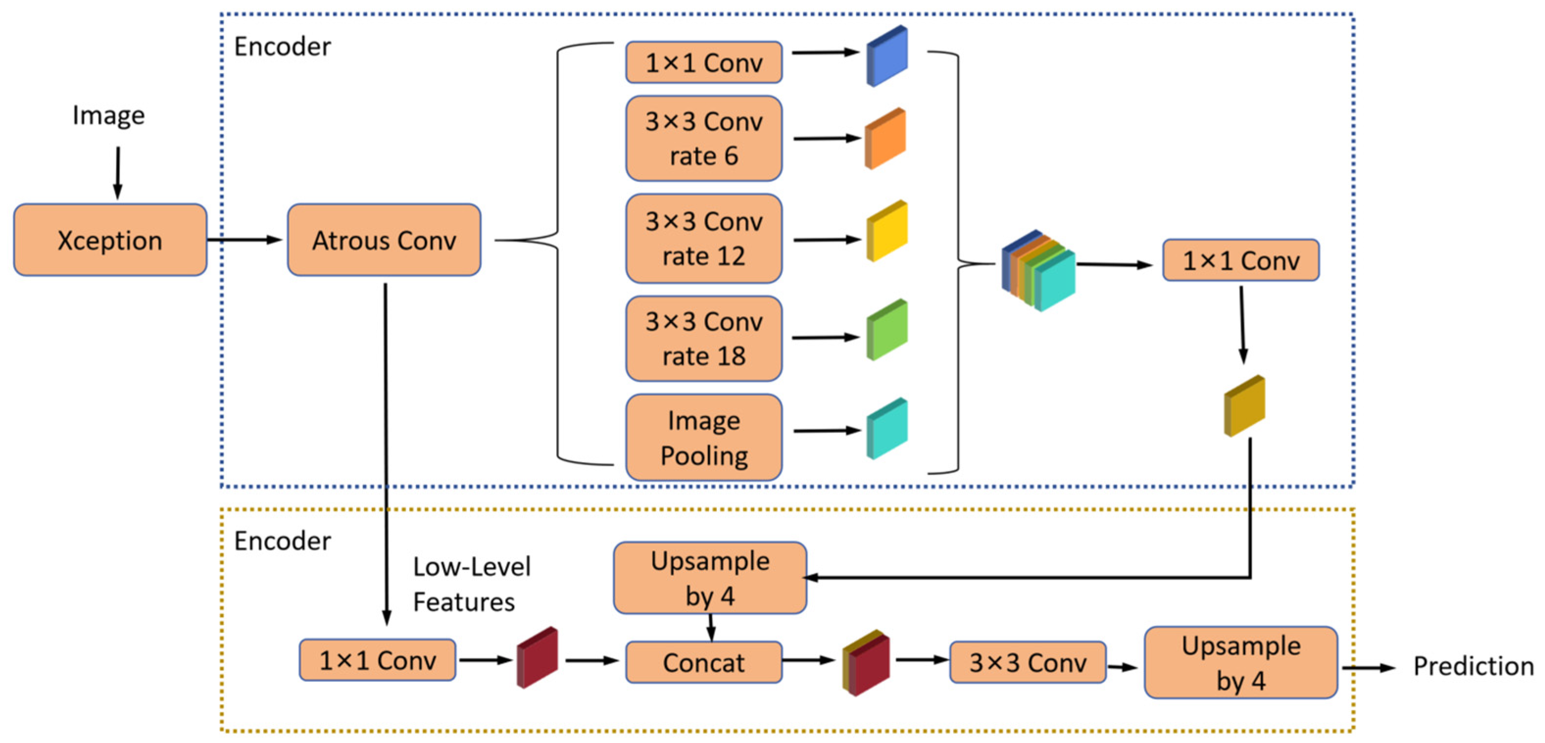
2.3.1. DeepLabV3+ Neural Network Model

As shown in Figure 4, DeepLabV3+ employs a deep convolutional neural network (DCNN) structure based on an encoder–decoder architecture [21]. The encoder uses a pre-trained deep convolutional network (Xception) as the backbone to extract high-level semantic information from the images. The feature maps outputted by the backbone network are processed by an Atrous Spatial Pyramid Pooling (ASPP) module to capture multi-scale contextual information. The backbone DCNN utilizes parallel Atrous Convolution to adjust the channel number of high-resolution feature maps through convolution operations. These are then concatenated with upsampled low-resolution feature maps and further convoluted to obtain the final segmentation results. After the image data pass through the backbone DCNN, the results are divided into two parts: one part is directly input into the decoder for computation, while the other part goes through parallel Atrous Convolution with different rates for feature extraction. The five results are merged and subjected to 1 × 1 convolution operations to compress features, enabling efficient and accurate classification of each pixel in the image. The decoder is responsible for restoring the spatial information of the image to achieve precise segmentation results.

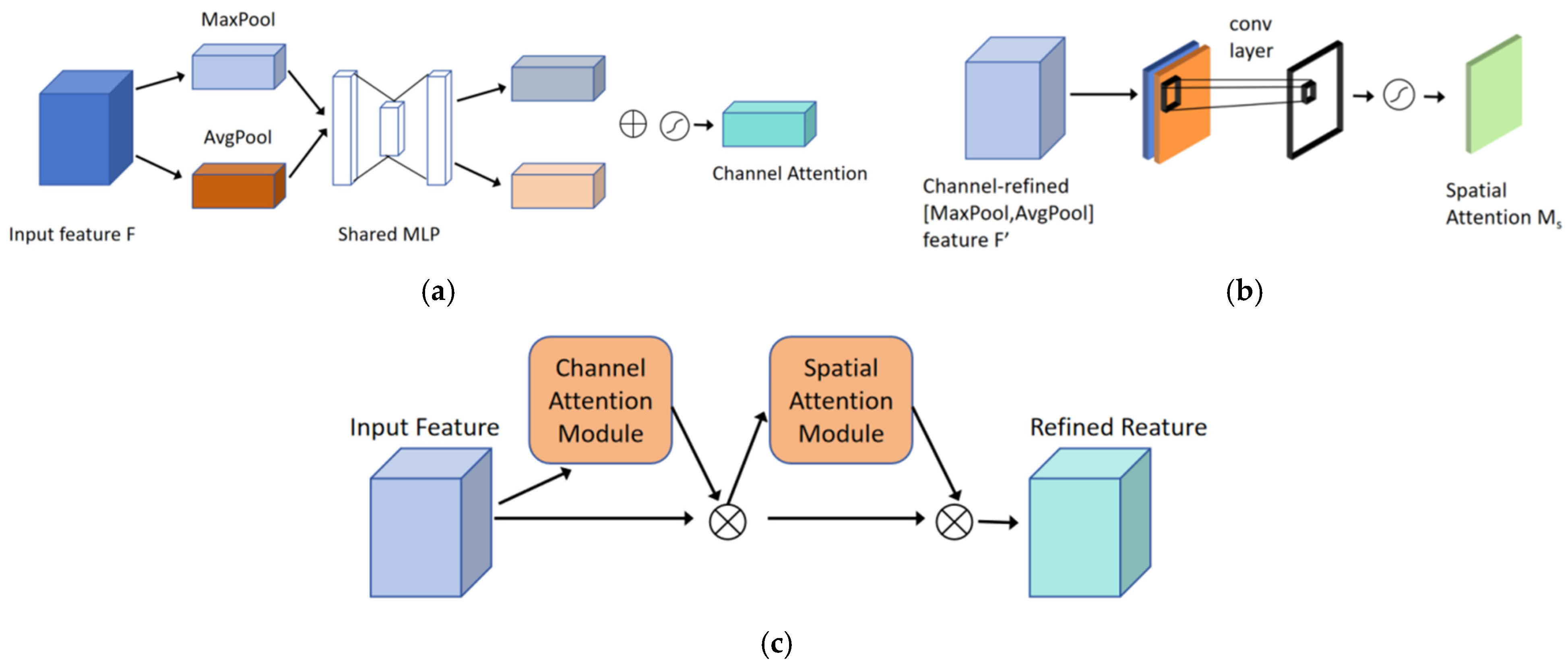
2.3.2. Attention Mechanism Module: CMAM

As shown in Figure 5, the CBAM (Convolutional Block Attention Module) is a lightweight attention module that consists of two sub-modules: CAM (Channel Attention Module) and SAM (Spatial Attention Module). These sub-modules focus on feature information in the channel and spatial domains, respectively [22].

The CAM enhances the feature representation of each channel by performing global max pooling (MaxPool) and global average pooling (AvgPool) operations on each channel of the input feature map. This process calculates the maximum and average feature values for each channel, generating two feature vectors that represent the global max and average features for each channel. These feature vectors are input into a shared multi-layer perceptron (Shared MLP), which learns the attention weights for each channel. The network adaptively determines important channels by performing an intersection calculation (⨁) between the global max feature vector and the average feature vector, resulting in the final attention weight vector. A Sigmoid activation function is then applied to produce the channel attention weights, which are multiplied by the corresponding channels of the original feature map to obtain the attention-weighted channel feature map—emphasizing channels that are helpful for the current task while suppressing irrelevant channels, thus achieving channel attention.

The SAM emphasizes the importance of features in different spatial positions within the image. It applies max pooling (MaxPool) and average pooling (AvgPool) operations across the channel dimension of the input feature map to generate contextual features at different scales. The features from the max pooling and average pooling operations are concatenated along the channel dimension to produce a feature map that contains contextual information at various scales. This feature map is then processed by a convolutional layer, and a Sigmoid activation function generates the spatial feature vector weights, constraining them between 0 and 1. The resulting spatial attention weights are applied to the original feature map, weighting the features at each spatial position to highlight important regions of the image while reducing interference from less important areas.

The CBAM combines the outputs of the CAM and the SAM through element-wise multiplication (⨂) to obtain the final enhanced features. These enhanced features serve as input data for subsequent layers of the network and improve the convolutional neural network’s ability to capture key features, thereby enhancing the accuracy of the predictions made by the semantic segmentation model DeeplabV3+. However, the CBAM increases the computational parameters of the DeeplabV3+ model; therefore, lightweight design techniques need to be applied to ensure the real-time performance of the mower.

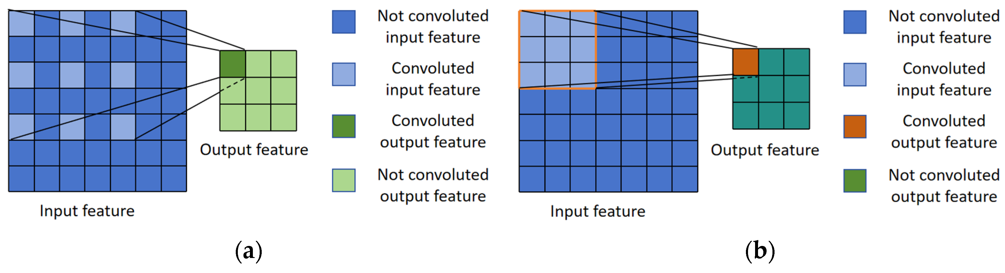
2.3.3. Lightweight Design by MobileNetV2

MobileNetV2 is an efficient neural network architecture designed for embedded devices. It enhances performance through a reverse residual structure and lightweight depthwise separable convolutions, allowing it to operate efficiently on resource-constrained devices while maintaining a relatively high level of accuracy [23,24].

As shown in Figure 6, the main components of MobileNetV2 are Inverted Residual Blocks and Linear Bottlenecks. In MobileNetV2, the input and output channel numbers are relatively low, while the intermediate depthwise separable convolution layers have a larger number of channels, forming an inverted bottleneck structure. The input data are first expanded in channel number through a 1 × 1 pointwise convolution, followed by feature extraction using a 3 × 3 depthwise separable convolution, and finally compressed back to the original channel number through another 1 × 1 pointwise convolution. In the Inverted Residuals structure, ReLU6 is used as the activation function. ReLU6 is a bounded version of the Rectified Linear Unit (ReLU) activation function, which constrains the output of ReLU between 0 and 6. The Stride = 1 Block utilizes skip connections to maintain the flow of information, reduce computational costs, and benefit gradient propagation. In the Inverted Residual structure, the last 1 × 1 convolution layer employs a linear activation function, allowing it to retain as much information integrity as possible during output. When the convolution kernel has a Stride = 1, it slides pixel by pixel, resulting in an output feature map size that is similar to that of the input feature map. In contrast, the Stride = 2 Block uses a larger step size for the convolution kernel, significantly reducing the size of the output feature map compared to the Stride = 1 Block. This helps to decrease computational costs and reduce model complexity, accelerating the training and inference processes of the model.

2.3.4. Improved DeeplabV3+ Model

The improved DeeplabV3+ model retains the structure of the Atrous Spatial Pyramid Pooling (ASPP) module. In the ASPP module of the original backbone network, the convolution path with a rate of 12 for the 3 × 3 kernel was removed while keeping the other dilated convolution paths, which reduces the computational burden of the neural network. The parallel dilated convolution layers with different dilation rates obtain feature maps with various receptive fields. These feature maps are then fused to obtain multi-scale target features. As shown in Figure 7, dilated convolutions, when extracting feature points, span across pixels. By increasing the receptive field without losing information, each convolution output incorporates a broader range of information, thereby enhancing the model’s efficiency in capturing input features.

In the encoder, the MobileNetV2 network replaces the Xception network. Xception parameters vary according to the specific configuration and input size of the model, and the order of magnitude of parameters may range from tens of megabytes to hundreds of megabytes. MobileNetV2 significantly makes the parameter amount about 3.4 megabytes through the deep separable convolution and reverse residual structure, which is much smaller than the Xception parameter amount. The residual connections in the MobileNetV2 architecture help the network learn deep features more effectively while avoiding the problems of vanishing and exploding gradients, which enhances the ability to capture edge features of connected regions. There are significant differences in spatial distribution and color classification among the four main objects in the orchard environment: weeds, fruit tree trunks, fruit tree leaves, and bare ground at the field’s edge. After concatenating the outputs of the encoder’s ASPP structure, a 1 × 1 convolution operation is performed, followed by the addition of a CBAM attention mechanism module to enhance the model’s ability to extract key spatial and channel information features of the four target categories in the orchard environment. The number of channels of the feature map after 1 × 1 convolution operation is C, and the channel attention module compresses the spatial dimension of the feature map to 1 using global average pooling and global maximum pooling to obtain two channel descriptors. The two channel descriptors perform feature transformation through a shared multi-layer perceptron (MLP), and the MLP is composed of two fully connected layers through the ReLU activation function. If the compression ratio of MLP is set to r, the number of output channels of the first full connection layer is c/r. Therefore, the parameter quantity of the first full connection layer is C × (c/r), and the parameter quantity of the second full connection layer is (c/r) × C. The parameter quantity of the channel attention module mainly comes from the first full connection layer and the second full connection layer. The parameter quantity is 2C²/r on the premise of ignoring the bias term. The spatial attention module performs channel wise maximum pooling and average pooling on the input feature map to generate two spatial descriptors. The two spatial descriptors are spliced in the channel dimension to obtain a feature map with 2 channels. The spatial attention map is generated by convolution layer operation with convolution kernel size of 7 × 7 and step size of 1. The parameters of spatial attention module mainly come from convolution layer, which is about 7 × 7 × 2 × 1 = 98. Therefore, the parameter computation of CBAM attention mechanism module is about 2C²/r + 98. A schematic diagram of the backbone network structure of the improved DeeplabV3+ model (ImDeeplabV3+) is shown in Figure 8.

The input image size for the ImDeeplabV3+ neural network is 1920 × 1080. The orchard environment image data is transmitted through various layers of the neural network to ultimately output the prediction results. After the camera mounted on the mower captures the image data, they are input into the neural network for semantic segmentation, extracting key information to generate environmental prediction images at each stage of the process, with four main object categories, grassland, leaf, freespace, and trunk, which are used to generate the navigation path.

2.4. Navigation Path Generation

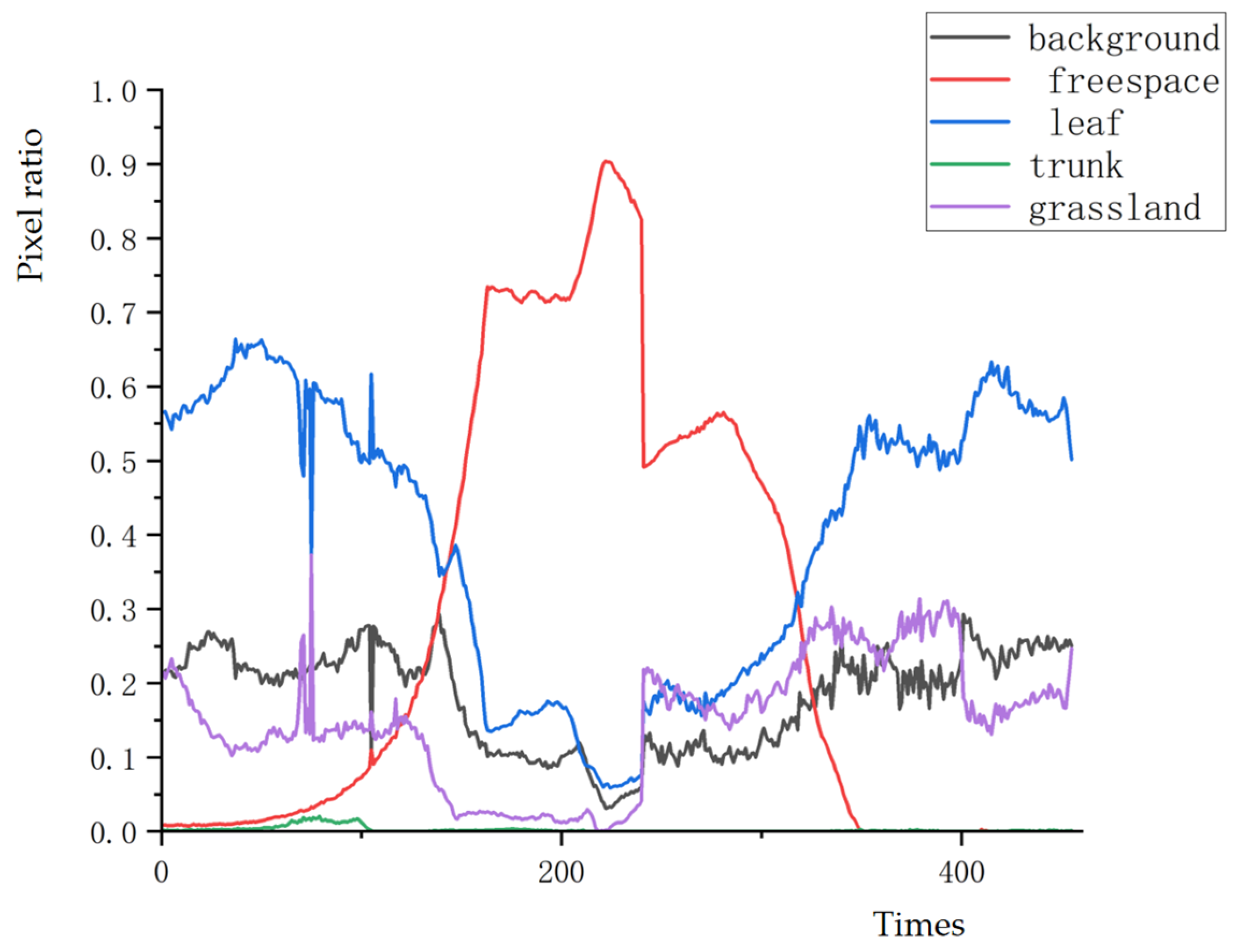
2.4.1. Semantic Segmentation Change Scenario

To determine the various stages of the mower’s progression, the camera mounted on the mower collected a total of 455 images throughout the process. The pixel count statistics for each region of the images labeled using LabelMe are shown in Figure 9.

During the progression of the mower, the pixels in the camera’s field of view dynamically change, and the area pixel statistics reflect the moments of stage transitions. In Figure 9, when the sampling range is [0, 121], the pixel proportion of the freespace category increases from 0.009 to 0.145, indicating the scenario where the mower is advancing to the edge of the field, defining this stage as Stage One. When the sampling range is [121, 147], the pixel proportion of the grassland category shows a decreasing trend, while the freespace category shows an increasing trend; at the 121st sample, the curves for the grassland and freespace pixel proportions intersect, with the intersection coordinates being (121, 0.145). This intersection is set as the turning point between Scenario One and Scenario Two, marking the transition of the navigation path generation method from Stage One to Stage Two. As the number of samples increases, the pixel proportion of the leaf category first decreases and then rises, with a change range of [0.06, 0.65]. During the sampling range of [163, 240], the leaf category pixel proportion remains at a lower level, indicating that the mower is in the second stage of the line switch, transitioning from the current line to the line change segment. When the pixel proportion of the freespace category is at a high level, within the sampling range of [163, 281], at the 163rd sample, the pixel proportions across the regions show a transition from Stage Two to Stage Three for the mower. When the sampling range is [242, 281], the pixel change trends across categories are stable, indicating that the mower has fully entered the line switch path, with the freespace pixel proportion being the highest. After the 281st sample, the pixel proportion of the freespace category shows a decreasing trend, while the leaf category pixel proportion shows an increasing trend, marking the transition from Stage Three to Stage Four, where the mower needs to complete a turn and enter the target line. At the 349th sample, the pixel proportion for the freespace category is 0, and the pixel proportion of the leaf category exhibits small changes in subsequent samples, indicating that the mower has entered the target line and completed the line switch task, switching the navigation path generation method to Stage Five. As shown in Figure 10, the improved semantic segmentation model DeeplabV3+ provides the segmentation results for each scenario as illustrated.

The resolution of the segmented image in Figure 10 is 1920 × 1080, where the width is 1920 pixels and the height is 1080 pixels. The connected regions of the image serve as the basis for generating the navigation path. During the cross-row process, the lawnmower utilizes machine vision technology, using the pixel occupancy information of grassland, leaf, freespace, and trunk as the basis for actions. In the segmented image, the green area represents grassland, the blue area indicates leaves, the red area denotes freespace, and the yellow area represents the trunk.

When processing large datasets, the K-means algorithm converges quickly to reduce the computational load. By applying the K-means clustering method, threshold values are set for different color channels, dividing the image pixels into four color clusters, and boundaries are drawn for each cluster to differentiate the connected regions. The centroid is the center of mass of the connected regions in the image, reflecting the distribution and characteristics of the clustered data. Determining the centroid’s position is crucial for planning navigation paths at different stages and provides data support for the decision-making system. The centroid is derived from the moments of the boundaries of different connected regions using the CV2.moments function, which returns a dictionary containing all calculated moments. The centroid of the connected regions serves as a key basis for generating navigation paths, with M00 being the zero-order moment representing the area of the connected region; M10 being the first-order moment about the X-axis; and M01 being the first-order moment about the Y-axis. The coordinates of the centroid are given by (Cx, Cy), where Cx = M10/M00 and Cy = M01/M00.

2.4.2. Navigation Path Generation Principle

The mower experiences five scenes during the row-changing process, establishing a Cartesian coordinate system with the camera position as the origin O. Figure 10 show the schematic diagram of the navigation path generation.

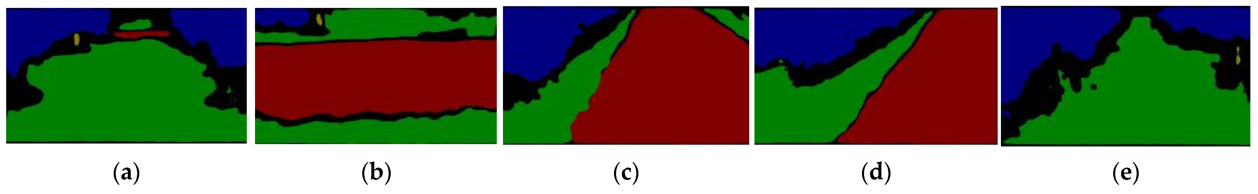
• Figure 10a illustrates the first stage of the row-changing process, where the lawnmower is moving between the current rows. The navigation path L1 for this stage is generated from the centroid A (x₁, y₁) of the grassland area between the current rows and the centroid B (x₂, y₂) of the freespace, with the calculation process described in formula below:

$$y={\displaystyle \frac{y_2-y_1}{x_2-x_1}}(x-x_1)+y_1$$

(2)

2.

In the formula, y₂ − y₁/x₂ − x₁ represents the slope of path L₁, and the navigation path L₁ in Stage One is expressed by the linear regression equation of y with respect to x.

3.

As shown in Figure 10b, the mower reaches the edge at the intersection of the current row and the next row, entering the second phase. The navigation path needs to guide the mower to make a turn to enter the next row. Equation (3) represents the generation expression for the navigation path in the second phase. The centroid B₁(x₃, y₃) of the freespace area during this phase has the auxiliary line l₂ parallel to the x-axis, and it connects to the centroid Q(x₄, y₄) of the grassland, forming line l₃. The navigation path for the mower in this phase is L₂, which is an arc-shaped path that is inscribed between l₃ and l₂. At this point, the mower deviates to the left from the current row to enter the next row. The calculation process for the inscribed circle of path L₂ is described in Equation (3), where A, B, D, E, C₁, and C₂ are parameters from the function equations of line segments l₂ and l₃, (x_o, y_o) represents the coordinates of the center of the arc for path L₂, and r denotes the radius of the arc:

$$\left\{\begin{array}{c}{l}_2:Ax+By+C_1=0\\ l_3:Dx+Ey+C_2=0\\ A(x-x_0)-B(y-y_0)=0\\ D(x-x_0)-E(y-y_0)=0\\ r={\displaystyle \frac{\left|A{x}_o+B{y}_o+C_1\right|}{\sqrt{A^2+B^2}}}\end{array}\right.$$

(3)

4.

As shown in Figure 10c, the tracked mower enters the third phase of the next row section. In this phase, the proportion of the freespace area is the largest, and the shape of the area is relatively regular, making it easier to generate the coordinates of the edge scatter points on the boundary of the freespace area. This phase uses a linear regression approach based on a least squares method to analyze the scatter points on both edges, calculating the linear equations for the left and right boundaries of the freespace area (l₄ and l₅). Using these two linear equations, the center point is calculated to generate the navigation path L₃ for entering the next row section:

$$\left\{\begin{array}{l}Y=a_0+a_{1}X\\ a_0={\displaystyle \frac{{\displaystyle \sum y_i}}{m}}-a_1{\displaystyle \frac{{\displaystyle \sum x_i}}{m}}\\ a_1={\displaystyle \frac{{\displaystyle \sum x_i{y}_i-\frac{{\displaystyle \sum x_i{y}_i}}{m}}}{{\displaystyle \sum x_i^2-\frac{{({\displaystyle \sum x_i})}^2}{m}}}}\\ R=\frac{{\displaystyle \sum x_i}{y}_i-m{\displaystyle \sum \frac{x_i}{m}{\displaystyle \sum \frac{y_i}{m}}}}{\sqrt{[{\displaystyle \sum x_i^2}-m{({\displaystyle \sum \frac{x_i}{m}})}^2][{\displaystyle \sum y_i^2}-m{({\displaystyle \sum \frac{y_i}{m}})}^2]}}\end{array}\right.$$

(4)

5.

In the equation, Y is the regression function concerning X, representing the relationship between the variables (x_i, y_i), where x_i and y_i are the coordinate values of the pixel points in the image. a₀ and a₁ are the correlation coefficients of the regression equation Y. R is the correlation coefficient used to assess the effectiveness of the data points in regression; the closer the value is to 1, the higher the correlation between the data points (x_i, y_i) and the regression equation. m represents the total number of sampled edge points in the connected regions of the image, and the linear equations for l4 and l5 are both represented by Equation (4).

6.

As shown in Figure 10d, the tracked mower is about to enter the target row at the turning endpoint. As the weedy area between the target rows gradually increases, the proportion of grassland pixel points in the image also increases. The principle for path L₄ is the same as that of path L₂; in this phase, the tracked mower must execute a turning maneuver to enter the target row, with the calculation method being described by Equation (3). The coordinates of point O are (960, 0), point B₂ is the centroid of the freespace area in this phase, and point A₁ is the centroid of the grassland area in this phase. Line l₆ is drawn through points A₁ and B₃, and line l₇ is drawn through points O and B₃. Path L₄ is an arc that is tangential to lines l₆ and l₇.

7.

In Figure 10e, the tracked mower enters the target row, and path L₅ represents the driving path of the mower after it has entered the target row. The calculation method for this path is the same as that for path L₃, described by Equation (4). In the figure, the linear equations for l₈ and l₉ are both regression functions of Y concerning X, and the line segment for the navigation path L₅ is defined by the midline equation determined by l₈ and l₉.

The tracked mower follows the paths of the five stages shown in Figure 11, with the automated row change control system adjusting the yaw angle based on the relationship between the navigation paths for each stage and the coordinates of the camera O on the mower. The acceleration of the tracked mower directly affects its yaw angle, which describes the angle of the mower’s rotation around its Z-axis in three-dimensional space, indicating the mower’s left and right deflection on the X–Y horizontal plane. During travel, the mower’s steering system controls the acceleration of the left and right tracks in accordance with the generated paths L₁–L₅, achieving automatic adjustment of the mower’s posture while following the path during the row-changing process.

2.5. Decision-Making Model for Automatic Turning of Orchard Tracked Mower

The key to enabling the tracked mower to automatically turn is the generation of navigation paths and path tracking control [25]. The ImDeeplabV3+ neural network identifies the orchard headland environment, constructing a semantic segmentation image environment model to generate navigation paths. The movement of the tracked mower is powered by a stepper motor, which adjusts the motor’s shaft speed to control the mower’s posture. The input parameters are determined by the relationship between the starting point of the navigation path O’ and the mower’s camera coordinates O. In the segmented image, the coordinates of point O are (x₀, y₀), while the coordinates of point O’ are (x_i, y_j), where −960 ≤ i ≤ 920 and 0 ≤ j ≤ 1080. As the mower moves, the coordinates of the navigation path starting point O’ change with the stages of the turning process. To ensure that the mower accurately follows the path, it is defined that within a path tracking period T, the coordinates of point O need to coincide with the coordinates of point O’ at the same moment t. The relationship between the O’ coordinates during path tracking and the expected coordinates of point O” (x_t, y_t) is represented by Formula (5):

$$\left\{\begin{array}{l}{W}_{11}={\displaystyle {\int }_{t_0}^{t}x\mathrm{dt}}=x_i-x_t\\ W_{12}={\displaystyle {\int }_{t_0}^{t}y\mathrm{dt}=y_j-y_t}\\ W_{21}={\displaystyle \frac{\arctan \frac{x_i-x_0}{y_j-y_0}-\alpha }{\omega }}\\ W_{22}={\displaystyle \frac{\arctan \frac{x_i-x_0}{y_j-y_0}-\beta }{\omega }}\end{array}\right.$$

(5)

In the formula, T = t − t₀, where x represents the lateral offset of the tracked mower per unit time, and y represents the longitudinal offset of the tracked mower per unit time. The automatic turning control system is illustrated in Figure 12.

In Equation (6), W₁₁, W₁₂, W₂₁, and W₂₂ are matrix parameters for dynamic input variables. The effect of controlling the track speed is achieved by regulating the left and right motor speeds, v_left and v_right, of the controlled object. The control matrix represents the relationship between system inputs and outputs, where the pixel coordinates of the image serve as system input variables. The computational formulas for path generation change as the tracked mower progresses through different stages. These stages are determined by the pixel ratio δ of various categories in the image, and the system’s control matrix adapts accordingly. The control matrix parameters are divided into three groups: C₁₁, C₁₂; C₂₁, C₂₂; and C₃₁, C₃₂, corresponding to the three navigation path calculation methods during the five stages of the line-following process. The calculation process for the left and right track motor speeds, v_left and v_right, is described by Equation (6):

$$\left\{\begin{array}{l}{v}_{left 1}=W_{11}{C}_{11}+W_{12}{C}_{12}\\ v_{right 1}=W_{21}{C}_{11}+W_{22}{C}_{12}\\ v_{left 2}=W_{11}{C}_{21}+W_{12}{C}_{22}\\ v_{right 2}=W_{21}{C}_{21}+W_{22}{C}_{22}\\ v_{left 3}=W_{11}{C}_{31}+W_{12}{C}_{32}\\ v_{right 3}=W_{21}{C}_{31}+W_{22}{C}_{32}\end{array}\right.$$

(6)

The DeeplabV3+ semantic segmentation model performs real-time segmentation of the RGB images in the line-following process environment. The predicted segmented images, containing semantic information, are input into the automatic line-following control system. This control system utilizes the pixel data from various category regions to determine the phase of the tracked mower in the line-following process and generates the corresponding navigation path for that phase. By calculating the desired adjustment based on pixel coordinates, the system outputs pulse control signals to adjust the track speed, enabling the tracked mower to follow the navigation path and complete the automatic line-following task in the orchard headland environment.

3. Results

3.1. Model Evaluation Metrics

3.1.1. Comparison of Semantic Segmentation Model Performance

The training loss value (Loss) and the validation loss value (Val_Loss) during the model training process can serve as criteria for selecting the best model [26,27]. Both the training loss value and the validation loss value consistently decrease over the course of training, resulting in gradual performance improvement of the model on the validation set. DeeplabV3+_Xce is the model of the backbone network using the Xception structure. And DeeplabV3+_Mob uses the MobileNetV2 structure as the backbone network. DeeplabV3+_Xce_CBAM embeds the CBAM attention mechanism module on the base of DeeplabV3+_Xce. The location of the CBAM in DeeplabV3+_Xce_CBAM is the same as in ImDeeplabV3+. All neural network models trained on the same orchard headland environment image dataset recorded the changes in both types of loss values during the training process, as shown in Figure 13.

The Loss of DeeplabV3+_Xce converged to a lower level at the 25th epoch. The Loss of DeeplabV3+_Mob converged to a lower level at the fifth epoch. The Loss of DeeplabV3+_Xce_CBAM finally converged to 0.0778, and it is 0.0082 lower than the final result of DeeplabV3+_Xce. The final Loss value of ImDeeplabV3+ model is 0.073, which is the smallest compared with other models. The Val_loss of DeeplabV3+_Xce converged to a lower level at the 37th epoch. The Val_Loss of DeeplabV3+_Mob converged to a lower level at the 14th epoch. The Val_Loss of DeeplabV3+_Xce_CBAM finally converged to 0.0469, and it is 0.0331 lower than the final result of DeeplabV3+_Xce. The final Val_Loss value of ImDeeplabV3+ model is 0.032, which is the smallest compared with other models.

Model training workstation parameters include the following: Intel i9 14900k processor, that was made by Intel which is located in California, USA, 64 GB RAM, 4 TB disk storage, and an RTX 4090 graphics card with 24 GB of VRAM that was made by NVIDIA which is located in Santa Clara, CA, USA. The training environment was set up using PyTorch 3.7 and employed the Adam optimizer, with a training cycle of 200 epochs. Each epoch saved the model weights, with a maximum learning rate of 0.1 and a minimum learning rate of 0.0001.

The coefficient of determination (R²) is used in statistics to quantify the goodness of fit of a model to the observed data. The closer the value is to 1, the better the model’s fit and the stronger the explanatory power of the independent variable over the dependent variable [28,29]. In this study, R² is employed to assess the predictive performance of each category area’s measurements (proportion of pixel count), with the evaluation parameter R² calculated using Equation (7):

$$R^2={\displaystyle \frac{{\displaystyle \sum {(y_b\prime -y_a)}^2}}{{\displaystyle \sum {(y_b-y_a)}^2}}}$$

(7)

In the equation, y_b represents the actual value of the b-th sample, y_b’ represents the predicted value of the b-th sample, and y_a represents the mean value of all samples. As shown in Figure 14, different models predict images of four category areas. The proportion range for the freespace area in the test images is [0, 0.9], for the grassland area is [0, 35], and for the leaf area is [0, 0.25]. The pixel count of the trunk area for fruit trees is near zero; therefore, the prediction performance of the model is evaluated using the freespace, grassland, and leaf areas. Five sets of proportion data for each category area are selected to test the model, with the chosen proportions all within their respective ranges.

To facilitate comparison of the model’s accuracy in recognition performance, the freespace area range is selected as [0, 0.75] with a step size of 0.15; the grassland area range as [0, 0.35] with a step size of 0.07; and the leaf area range as [0, 0.25] with a step size of 0.05.

Figure 14 shows a comparison of the semantic segmentation model DeeplabV3+ before and after improvement. The improved ImDeeplabV3+ model fits the expected values better in predicting the pixel proportions of various connected areas. The R² values of models reflect their prediction performance, with statistics shown in Figure 15a. A higher accuracy means that the semantic segmentation model has stronger capabilities in feature extraction and classification decisions. In an automatic turning control system, the semantic segmentation model can accurately identify each category of area as a key element, providing precise environmental perception for the tracked mower’s automatic turning system, thereby increasing the passage rate. During the image prediction process, semantic segmentation models can produce certain errors. This study uses manually annotated images as a standard to calculate the average pixel accuracy P_M of predicted images for each network model to assess the segmentation effect of the network, as represented by Formula (8).

$$P_M={\displaystyle \frac{1}{N}}{\displaystyle \sum _{i=1}^N\frac{n_{ii}}{u_i}}\times 100\%$$

(8)

In the formula, N represents the number of categories; n_ii is the number of pixels of category i that are correctly predicted as category; and u_i is the number of pixels of category i in the ground-truth labels.

Figure 15 shows the average accuracy of the predictions for each area made by different neural network models on 400 labeled images.

All four types of neural network model are semantic segmentation models. The ImDeeplabV3+ model predicts the average accuracy of the three types of connected areas—freespace, grassland, and leaf—at 91.14%, 91.37%, and 93.01%, respectively, which is the highest average accuracy compared to the other three models.

Figure 16 shows the prediction results of models on RGB images at each stage of the mower moving process. Compared with others, the improved ImDeeplabV3+ model has the best prediction effect on images. And it predicts the continuity of various connected regions in the images the best. The images’ boundary segmented by the improved ImDeeplabV3+ model is the clearest. The accurate image segmentation ability of the model is the key to generate the navigation paths.

3.1.2. Path Tracking Effect

Let k be the slope of the regression function at point O with coordinates (x₀, y₀) and point O’ with coordinates (x_i, y_j). The yaw angle is given by the arctangent of the reciprocal of k, with the calculation formula being Formula (9):

$$\left\{\begin{array}{l}k={\displaystyle \frac{y_j-y_0}{x_i-x_0}}\\ \theta =\arctan ({\displaystyle \frac{1}{k}})\end{array}\right.$$

(9)

The manually labeled data regression-generated navigation line in this article is regarded as the ground truth, which is compared with the predicted values generated by data regression. We calculate the average deviation of the yaw angle and the average difference in the position of the yaw line. The calculation of the average yaw angle is given by Formula (10). The θ_t is the ground truth yaw angle at time t, θ_t^’ is the predicted value at time t, and θ represents the average deviation in yaw angle.

$$\theta ={\displaystyle \frac{1}{n}}{\displaystyle {\sum }_t\left|({\theta }_t-{{\theta }_t}^{\prime })\right|}$$

(10)

The tracked mower is equipped with an automatic turning control system that collects the environment at the orchard headland in real time. Based on the pixel ratio of key areas, it automatically switches working phases and generates adaptive navigation paths, controlling the left and right track speeds to adjust the yaw angle of the mower. The statistical results of the average deviation of the yaw angles for each neural network model during the various phases of the mower’s turning process are shown in

Table 1. Yaw angle statistics for different phases of the turning process for each model.

Model	Yaw Angle Deviation/°
	Current Line	Starting Point	Road Break	Ending Point	Target Line	Average Gap Between Lines
PSPNet	1.436	2.634	1.562	3.211	1.713	2.111
U-Net	1.271	2.188	0.935	2.212	0.983	1.518
DeeplabV3+_Xce	1.266	2.176	0.947	2.332	0.973	1.539
DeeplabV3+_Mob	1.197	2.088	0.914	2.157	0.962	1.464
DeeplabV3+_Xce_CBAM	0.986	1.899	0.992	1.837	0.989	1.394
ImDeeplabV3+	0.932	1.801	0.959	1.622	0.983	1.259

.

From Table 1, it can be seen that the average yaw angle deviation at various stages of the turning process for the models PSPNet, U-Net, DeeplabV3+_Xce, DeeplabV3+_Mob, DeeplabV3+_Xce_CBAM, and ImDeeplabV3+ are 2.111°, 1.518°, 1.539°, 1.464°, 1.394°, and 1.259°, respectively. ImDeeplabV3+ shows the smallest yaw angle difference across all stages, ensuring effective tracking of the navigation path during the turning process of the tracked mower. Compared to the other three stages, the average yaw angle differences are larger at the starting and ending points of the turn. The navigation paths at these two stages are curved, and the significant variation in pixel proportions of key areas in the images affects the precision of the control system’s adjustment of the tracked speed, leading to an increase in the average yaw angle difference.

3.2. Automatic Turning Experiment of the Tracked Mower

To verify the performance of the ImDeeplabV3+ model in the automatic turning system of the tracked mower, an experiment was conducted on 15 September 2024, at the First Station of the Taihang Mountains in Shunping County, Baoding City, Hebei Province, China. Figure 17 shows the working scene of the G33 tracked orchard mower during automatic turning.

The orchard used for the test is a modern, densely planted, low-stem orchard, with a row spacing of 2 m and a turning road width of 1.5 m. The G33 tracked mower is powered by a battery, and its basic structural parameters are shown in

Table 2. Structural parameters of the G33 tracked mower.

Mower	Parameters
Model	G33
Length × width × height	1.07 m × 0.98 m × 0.44 m
Linear velocity	1.5 m/s
Angular velocity	0.2 rad/s

. A camera continuously captures the surrounding orchard environment, transmitting RGB environmental images to the processor at a maximum transfer rate of 60 FPS and a resolution of 1920 × 1080. The neural network model is deployed in the NVIDIA Jetson Xavier NX module, with the processor having 16 GB of RAM to ensure the normal computation of the neural network.

In actual road tests, various models identify images of the orchard environment and generate navigation paths, controlling the vehicle’s posture to track the navigation path and achieve automatic turning at the end of the row. To assess the performance of the automatic turning system, the response speed and pass rate of mowers equipped with different model control systems are tested. To ensure the accuracy of the experimental results, the tracked mower undergoes turning tests 100 times, with a total path length of 15 m. The results of these experiments are summarized in

Table 3. Experimental results of mower line switching using different neural network models.

Model	MIoU	FPS	Passing Rate/%	Mean Transit Time/s
PSPNet	0.735	15.635	12	38.49
U-Net	0.826	20.148	77	30.81
DeeplabV3+_Xce	0.807	20.148	75	31.22
DeeplabV3+_Mob	0.823	58.656	78	10.97
DeeplabV3+_Xce_CBAM	0.915	18.384	87	34.52
ImDeeplabV3+	0.934	45.897	94	12.58

.

The MIoU is calculated for three key area pixel categories: freespace, grassland, and leaf. The pixel accuracy for each category is computed separately, and the average is taken to alleviate the class imbalance issue. The image processing speed is determined based on the time taken for every 100 frames of images, with the average passing time recorded only for successfully completed line switch tests.

4. Discussion

• In the second and fourth phases, the navigation path generated by the line switch decision model for the tracked mower is curved based on the surrounding environment. The average deviation of the yaw angle for these two phases is significantly larger compared to the other three phases. The navigation paths in the other three phases can be generated using information from a single type of area. The parameters required for the calculation of the curved navigation path come from the information on the freespace and grassland areas. Therefore, the increase in segmentation categories from the semantic segmentation model leads to a certain degree of decline in classification accuracy. This complexity in generating curved paths affects the guiding function of the expected navigation path, making it difficult for the automatic line switching control system to adjust the mower’s posture. LiDAR can obtain radar detection data from different areas, and by measuring the time difference between the emitted and received signals, it can determine the distance, orientation, and shape of the target. Combining LiDAR point cloud data with rich semantic segmentation image features is more beneficial for planning paths that map to real-world scenarios, further enhancing the tracked mower’s tracking performance on curved paths. At the same time, the environmental information acquisition system needs laser radar to detect the obstacles in the surrounding environment, such as stones, broken branches, and metal parts, to assist the mower in realizing the function of automatic obstacle avoidance and to avoid damage to the mower.
• In this study, the line switching road in the third phase is a concrete surface, while the line switching road in the orchard headland environment consists of non-concrete surfaces. To improve the robustness of the automatic line switching decision model for the mower in the orchard headland environment, it is necessary to further enrich the dataset used for training the semantic segmentation model. Additionally, the recognition strategy of the semantic segmentation model can be improved by optimizing the feature vectors. By integrating color features, texture features, and shape features into a comprehensive feature vector, more information can be captured, which will help the neural network model classify line change roads in different environments and enhance the transferability of the automatic line change decision model. The method of multi-type data enhancement is beneficial to improve the robustness and generalization of the model. Because the mower works outdoors, the future model design should consider how to improve the anti-interference ability of the model. Therefore, the collected data should include images under different lighting conditions. Data enhancement can also be achieved by changing the contrast of the image to simulate different lighting conditions.
• The straight-line travel and automatic line switching strategies of mowers need to be further optimized according to their own mowing width and orchard row width. In this study, the automatic line switching decision-making model of the mower does not enter the same working line repeatedly. When the mower’s mowing range is less than the fruit tree row width, the mower needs to enter the task row for the second time or even many times to complete the full-coverage mowing task. Therefore, the decision model is required to automatically divide the mower’s travel lane in the operation row according to the mower’s mowing width and the orchard row width to ensure that the mower can enter the working row many times. The designer may adjust the mowing width of the mower according to the inter-row width so that the mower can complete the task of the working line at one time. And we need to ensure that the mower can complete the task of mowing in the process of normal travel. Depth images assign a value representing the distance to each pixel, reflecting the three-dimensional structure of the scene. Utilizing the depth data from the images can supplement the distance information of the surrounding environmental areas, providing data for the mower’s travel control decision model. This enables precise adjustment of the tracked speed, allowing for the delineation of driving lanes between rows in the orchard, ensuring full coverage cutting, and reducing the occurrence of missed spots.

5. Conclusions

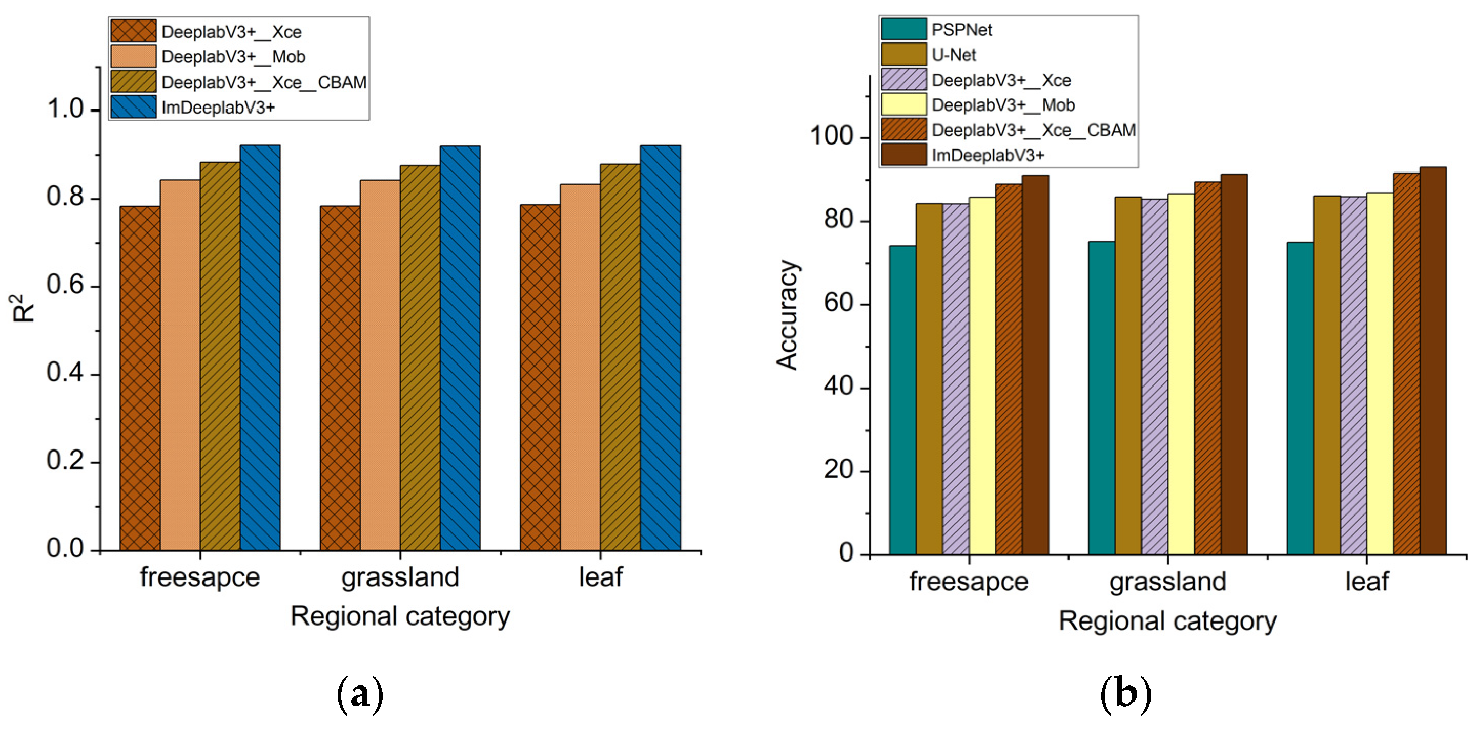
• DeeplabV3+_Xce, DeeplabV3+_Mob, DeeplabV3+_Xce_CBAM, and ImDeeplabV3+ constitute the ablation tests. The Loss value and the Val_Loss value of DeeplabV3+_Mob decreased faster than DeeplabV3+_Xce. The results of the automatic line change tests show that the DeeplabV3+_Mob semantic segmentation model achieves a speed improvement of 39.318 FPS compared to DeeplabV3+_Xce, with an average pass time reduction of 20.25 s. These show that Mobilenet V2 improves the computational efficiency of the model. The final Loss value and the Val_Loss of DeeplabV3+_Xce_CBAM were all smaller than those of DeeplabV3+_Xce. The DeeplabV3+_Xce_CBAM semantic segmentation model shows an improvement of 0.09 in average R² compared to DeeplabV3+_Xce, an increase of 5.0% in average accuracy, a reduction of 0.145° in average yaw angle deviation, and an increase of 10.8% in average intersection over union (MIoU). These show that the CBAM improves the classification accuracy of the model. The training loss value (Loss) and validation loss value (Val_Loss) for the ImDeeplabV3+ model are minimized at 0.073 and 0.032, respectively. Compared with other models, ImDeeplabV3+ has the best convergence effect.
• The results of the automatic line change tests show that the ImDeeplabV3+ semantic segmentation model achieves a speed improvement of 27.513 FPS compared to DeeplabV3+_Xce_CBAM, with an average pass time reduction of 21.94 s. The image processing efficiency of ImDeeplabV3+ is lower than that of DeeplabV3+_Mob by 21.75%. This suggests that the combination of MobileNet V2, the CBAM model, and the improved parallel Atrous Convolution structure enables the ImDeeplabV3+ model to effectively complete the automatic line switching task.
• The ImDeeplabV3+ semantic segmentation model enables relatively accurate classification of various targets in the unstructured orchard headland environment. The automatic line change control system plans a navigation path based on the semantic segmentation image data, controls the tracked speed, and adjusts the mowing posture to complete the automatic line change task, providing a design reference for decision models in the unmanned operation of tracked mowers.

References

1. Yan, W.; De, C.; Zhao, S. Unstructured road detection and tracking based on monocular vision. J. Harbin Eng. Univ. 2011, 32, 334–339. [Google Scholar]
2. Hou, K.; Sun, H.; Jia, Q.; Zhang, Y. An autonomous positioning and navigation system for spherical mobile robot. Procedia Eng. 2012, 29, 2556–2561. [Google Scholar] [CrossRef]
3. Xue, J.L.; Grift, T. Agricultural robot turning in the headland of corn fields. Appl. Mech. Mater. 2011, 63, 780–784. [Google Scholar] [CrossRef]
4. Li, J.; Chen, B.; Liu, Y. Image Detection Method of Navigation Route of Cotton Plastic Film Mulch Planter. Trans. Chin. Soc. Agric. Mach. 2014, 45, 40–45. [Google Scholar]
5. Liang, H.; Chen, B.; Jiang, Q.; Zhu, D.; Yang, M.; Qiao, Y. Detection method of navigation route of corn harvester based on image processing. Trans. Chin. Soc. Agric. Eng. 2016, 32, 43–49. [Google Scholar]
6. Lai, H.; Zhang, Y.; Zhang, B.; Yin, Y.; Liu, Y.; Dong, Y. Design and experiment of the visual navigation system for a maize weeding robot. Trans. Chin. Soc. Agric. Eng. 2023, 39, 18–27. [Google Scholar]
7. Li, Y.; Xu, J.; Wang, M.; Liu, D.; Sun, H.; Wang, X. Development of autonomous driving transfer trolley on field roads and its visual navigation system for hilly areas. Trans. Chin. Soc. Agric. Eng. 2019, 35, 52–61. [Google Scholar]
8. Yang, Y.; Zhang, L.; Zha, J.; Wen, X.; Chen, L.; Zhang, T.; Dong, Y.; Yang, X. Real-time extraction of navigation line between corn rows. Trans. Chin. Soc. Agric. Eng. 2020, 36, 162–171. [Google Scholar]
9. Le, Y.; Bengio, Y.; Hinton, G. Deep learning. Nature 2015, 521, 436–444. [Google Scholar]
10. Saleem, M.; Potgieter, J.; Arif, K. Automation in agriculture by machine and deep learning techniques: A review of recent developments. Precis. Agric. 2021, 22, 2053–2091. [Google Scholar] [CrossRef]
11. Kamilaris, A.; Prenafeta-Boldú, F. A review of the use of convolutional neural networks in agriculture. J. Agric. Sci. 2018, 156, 312–322. [Google Scholar] [CrossRef]
12. Zhong, C.; Hu, Z.; Li, M.; Li, H.; Yang, X.; Liu, F. Real-time semantic segmentation model for crop disease leaves using group attention module. Trans. Chin. Soc. Agric. Eng. 2021, 37, 208–215. [Google Scholar]
13. Zhang, X.; Gao, H.; Zhao, J.; Zhou, M. Overview of deep learning intelligent driving methods. J. Tsinghua Univ. (Sci. Technol.) 2018, 58, 438–444. [Google Scholar]
14. Lin, J.; Wang, W.; Huang, S. Learning based semantic segmentation for robot navigation in outdoor environment. In Proceedings of the 2017 Joint 17th World Congress of International Fuzzy Systems Association and 9th International Conference on Soft Computing and Intelligent Systems (IFSA-SCIS), Otsu, Japan, 27–30 June 2017; pp. 1–5. [Google Scholar]
15. Song, G.; Feng, Q.; Hai, Y.; Wang, S. Vineyard Inter-row Path Detection Based on Deep Learning. For. Mach. Woodwork. Equip. 2019, 47, 23–27. [Google Scholar]
16. Li, Y.; Xu, J.; Liu, D.; Yu, Y. Field road scene recognition in hilly regions based on improved dilated convolutional networks. Trans. Chin. Soc. Agric. Eng. 2019, 35, 150–159. [Google Scholar]
17. Lin, Y.; Chen, S. Development of navigation system for tea field machine using semantic segmentation. IFAC-PapersOnLine 2019, 52, 108–113. [Google Scholar] [CrossRef]
18. Badrinarayanan, V.; Kendall, A.; Cipolla, R. Segnet: A deep convolutional encoder-decoder architecture for image segmentation. IEEE Trans. Pattern Anal. Mach. Intell. 2017, 39, 2481–2495. [Google Scholar] [CrossRef]
19. Kang, J.; Liu, L.; Zhang, F.; Shen, C.; Wang, N.; Shao, L. Semantic segmentation model of cotton roots in-situ image based on attention mechanism. Comput. Electron. Agric. 2021, 189, 106370. [Google Scholar] [CrossRef]
20. Liu, L.; Wang, X.; Liu, H.; Li, J.; Wang, P.; Yang, X. A Full-Coverage Path Planning Method for an Orchard Mower Based on the Dung Beetle Optimization Algorithm. Agriculture 2024, 14, 865. [Google Scholar] [CrossRef]
21. Shen, C.; Liu, L.; Zhu, L.; Kang, J.; Wang, N.; Shao, L. High-throughput in situ root image segmentation based on the improved DeepLabv3+ method. Front. Plant Sci. 2020, 11, 576791. [Google Scholar] [CrossRef]
22. Woo, S.; Park, J.; Lee, J.; Kweon, I. Cbam: Convolutional block attention module. In Proceedings of the European Conference on Computer Vision (ECCV), Munich, Germany, 8–14 September 2018; pp. 3–19. [Google Scholar]
23. Sandler, M.; Howard, A.; Zhu, M.; Zhmoginov, A.; Chen, L.C. Mobilenetv2: Inverted residuals and linear bottlenecks. In Proceedings of the IEEE Conference on Computer Vision and Pattern Recognition, Salt Lake City, UT, USA, 18–23 June 2018; pp. 4510–4520. [Google Scholar]
24. Singh, P.; Kumar, D.; Srivastava, A. A CNN Model Based Approach for Disease Detection in Mango Plant Leaves; Springer Nature: Singapore, 2023; pp. 389–399. [Google Scholar]
25. Liu, L.; Wang, X.; Yang, X.; Liu, H.; Li, J.; Wang, P. Path planning techniques for mobile robots: Review and prospect. Expert Syst. Appl. 2023, 227, 120254. [Google Scholar] [CrossRef]
26. Chen, J.; Ma, B.; Ji, C.; Zhang, J.; Feng, Q.; Liu, X.; Li, Y. Apple inflorescence recognition of phenology stage in complex background based on improved YOLOv7. Comput. Electron. Agric. 2023, 211, 108048. [Google Scholar] [CrossRef]
27. Li, S.; Zhang, S.; Xue, J.; Sun, H. Lightweight target detection for the field flat jujube based on improved YOLOv5. Comput. Electron. Agric. 2022, 202, 107391. [Google Scholar] [CrossRef]
28. Zhang, J.; Wang, X.; Liu, J.; Zhang, D.; Lu, Y.; Zhou, Y.; Sun, L.; Hou, S.; Fan, X.; Shen, S.; et al. Multispectral drone imagery and SRGAN for rapid phenotypic mapping of individual chinese cabbage plants. Plant Phenomics 2022, 2022, 0007. [Google Scholar] [CrossRef]
29. Ye, Z.; Yang, K.; Lin, Y.; Guo, S.; Sun, Y.; Chen, X.; Lai, R.; Zhang, H. A comparison between Pixel-based deep learning and Object-based image analysis (OBIA) for individual detection of cabbage plants based on UAV Visible-light images. Comput. Electron. Agric. 2023, 209, 107822. [Google Scholar] [CrossRef]
Figure 1. Kinematic model of the track-type mower.
Agriculture 15 00647 g001
Figure 2. Headland environmental of orchard.
Agriculture 15 00647 g002
Figure 3. Mower line switching scenarios: (a) current inter-row; (b) turning start point; (c) turning path; (d) turning end point; (e) target inter-row.
Agriculture 15 00647 g003
Figure 4. DeepLabV3+ neural network model.
Agriculture 15 00647 g004
Figure 5. CBAM: (a) CAM; (b) SAM; (c) CBAM.
Agriculture 15 00647 g005
Figure 6. Neural network architecture of MobileNetV2.
Agriculture 15 00647 g006
Figure 7. The receptive fields of dilated convolution and ordinary convolution: (a) dilated convolution; (b) ordinary convolution.
Agriculture 15 00647 g007
Figure 8. ImDeeplabV3+ model.
Agriculture 15 00647 g008
Figure 9. Pixel category statistics during the line switch process.
Agriculture 15 00647 g009
Figure 10. Mower line switching scene segmentation result: (a) current inter-row; (b) turning start point; (c) turning path; (d) turning end point; (e) target inter-row.
Agriculture 15 00647 g010
Figure 11. The principle of generating the navigation paths in the five stages of the row-changing process: (a) First stage, between the current rows; (b) Second stage, turning start point; (c) Third stage, turning road; (d) Fourth stage, turning endpoint; (e) Fifth stage, between the target rows; (f) Overview schematic of the five-stage navigation path.
Agriculture 15 00647 g011
Figure 12. Automatic line wrapping control system.
Agriculture 15 00647 g012
Figure 13. The training Loss and Val_Loss: (a) Loss; (b) Val_Loss.
Agriculture 15 00647 g013
Figure 14. Comparison of prediction performance between DeeplabV3+_Xce, DeeplabV3+_Mob, DeeplabV3+_Xce_CBAM, and ImDeeplabV3+ models: (a) the predicted pixel proportion for the freespace connected area; (b) the predicted pixel proportion for the leaf connected area; (c) the predicted pixel proportion for the grassland connected area.
Agriculture 15 00647 g014
Figure 15. Comparison of model performance: (a) R2; (b) accuracy.
Agriculture 15 00647 g015
Figure 16. Prediction results of the models on the images.
Agriculture 15 00647 g016
Figure 17. Automatic turning test of the tracked mower.
Agriculture 15 00647 g017