Canopy-Level Rice Yield and Yield Component Estimation Using NIR-Based Vegetation Indices

Abstract

Accurately predicting rice yield and its components is crucial for optimizing agricultural practices and ensuring food security. Traditional methods of assessing crop status wwcan be time-consuming and labor-intensive. This study investigated the use of drone-based multispectral imagery and machine learning to improve the prediction of rice yield and yield components. Time-series VIs were collected from 152 rice samples across various nitrogen treatments, transplanting times, and rice varieties in 2023 and 2024, using an UAV at approximately 3-day intervals. A four-parameter log-normal model was applied to analyze the VI curves, effectively quantifying the maximum value, spread, and baseline of each index, revealing the dynamic influence of nitrogen and transplanting timing on crop growth. Machine learning regression models were then used to predict yield and yield components using the log-normal parameters and individual VIs as input. Results showed that the maximum (a) and variance (c) parameters of the log-normal model, derived from the VI curves, were strongly correlated with yield, grain number, and panicle number, emphasizing the importance of mid-to-late growth stages. Among the tested VIs, NDRE, LCI, and NDVI demonstrated the highest accuracy in predicting yield and key yield components. This study demonstrates that integrating log-normal modeling of time-series multispectral data with machine learning provides a powerful and efficient approach for precision agriculture, enabling more accurate and timely assessments of rice yield and its contributing factors.

1. Introduction

Rice is a staple crop that is consumed as a primary food source by more than half of the global population and is critical in ensuring global food security [1]. Advancements in precision agriculture have highlighted the importance of technological approaches to accurately predict rice yields [2,3]. The methods for estimating rice yield can be categorized into three primary approaches: crop growth modeling, statistical yield estimation, and remote sensing [4,5].

Remote sensing using satellite data can capture data over large areas using sensors capable of detecting various spectral bands [6]. Studies utilizing the moderate resolution imaging spectroradiometer normalized difference vegetation index (MODIS NDVI) to estimate actual rice yields have employed various methods, resulting in highly accurate yield prediction models [7,8]. However, satellite imagery has limitations such as susceptibility to wavelength interference caused by clouds and lower resolution, making it difficult to provide detailed field-level data [9]

Proximal sensing technologies such as unmanned aerial vehicles (UAVs) have gained attention to address these limitations. UAVs can efficiently collect high-resolution spatial and temporal data, making them a key solution in precision agriculture [10,11]. Multispectral data collected using UAVs are effective in quantitatively assessing field and crop growth conditions [12,13]. Vegetation indices (VIs) such as the normalized difference vegetation index (NDVI), green normalized difference vegetation index (GNDVI), normalized difference red edge index (NDRE), and leaf chlorophyll index (LCI), derived from UAV data, are extensively used for evaluating crop health, chlorophyll content, and biomass at the field level [14,15]. Recent studies have utilized various VIs as input variables in machine learning models to assess crop nutritional status and deficiencies [16].

Recent attempts have leveraged these capabilities to estimate crop yields at the field or community level using VIs collected by UAVs. Zhou et al. [17] developed regression models to estimate yield using VIs measured during the critical growth stages of three rice varieties across four planting densities. The study found the highest coefficient of determination (R² = 0.75) for NDVI during the tillering stage. However, they identified potential issues, such as overestimating early VIs owing to planting density, missing growth stage information, and reliance on data from a single year, which could introduce errors in yield estimation. Similarly, Duan et al. [18] developed a yield estimation model by analyzing multispectral indices from UAV imagery of nitrogen-treated rice samples. The model achieved an R² of 0.6 and a relative root mean square error (rRMSE) of <10%. However, they compared VIs from specific dates representing each growth stage without accounting for the variability in the growth cycle influenced by variety and weather conditions, which could have introduced errors. Bian et al. [19] constructed a regional regression model for predicting winter wheat yield using machine learning methods and multispectral UAV data. Ten VIs acquired at five key growth stages (jointing, heading, flowering, filling, and milk-ripe stages) were used as variables in six machine learning models (GPR, SVR, RFR, DT, Lasso, and GBRT). The GPR model showed the highest accuracy (R² = 0.87) at the filling stage. However, further study is needed to address the potential variability in growth stages due to weather conditions and cultivar characteristics.

Therefore, the study aimed to analyze four rice varieties with different nitrogen treatments and transplanting times under a uniform planting density to address the abovementioned limitations. Multispectral imagery was captured at approximately 3-day intervals, and six types of time-series VIs were extracted from 152 samples. By capturing data across multiple growth stages, the indices were fitted to a log-normal distribution with four parameters, enabling continuous values and visualizing graphical pattern changes based on nitrogen treatment, transplanting time, and variety. Furthermore, the parameters of the log-normal distribution were used as input variables in a machine learning-based multiple regression model to estimate the yield using time-series VI data for the entire growth period. This approach provides a robust method for predicting the rice yield.

2. Materials and Methods

2.1. Experimental Setup

This study was conducted in 2023 and 2024 at the National Institute of Crop Science (NICS) in Wanju, South Korea (35.96° N, 127.05° E) using field and soil bin environments (Figure 1A). The climate information of the region in 2023 and 2024 is presented in Figure 1B. The soil bins measured 1 × 1 × 0.5 m and were placed outdoors for plant growth. In 2023, field transplantation was conducted on 7 and 26 June, with the latter defined as the late transplantation (LT) treatment. Soil bin transplantation was performed on 9 June. In 2024, field transplanting was conducted on June 8, whereas soil bin transplanting occurred on June 10. The planting distance was uniformly set at 30 × 14 cm for all samples. For the field environments, machine transplanting was used, whereas soil bins were hand-transplanted with three plants per hill. Plants were cultivated and managed according to the standard rice cultivation practices of the NICS Rural Development Administration. The primary cultivar used was Nampyeong (NP). However, in 2024, additional cultivars, including Dongjin-1(DJ), Shindongjin (SD), and Saeilmi (SI), were introduced to evaluate varietal responses under the specified treatment conditions.

2.2. Treatment Conditions

Nitrogen fertilizer was applied at 0, 98.8, and 197.6 kg/ha. Each treatment condition was established based on year, environment (field or soil bin), nitrogen level, and cultivar (

Table 1. Experimental treatment conditions by growth environment, transplanting date, cultivar, and nitrogen treatment.

	Growth Environment	Transplanting Date	Cultivar	Nitrogen Fertilizer (N, kg·ha−1)	Sample Number	Harvest Date	Treatment (Acronyms)
2023	Field	June 7	Nampyeong	0	5	October 18	23-F-0N
				98.8	5	October 18	23-F-9N
		June 26	Nampyeong	0	5	October 18	23-F-0N-LT
				98.8	5	October 18	23-F-9N-LT
	Soil bin	June 9	Nampyeong	0	8	October 18	23-S-0N
				98.8	8	October 18	23-S-9N
				197.6	8	October 18	23-S-18N
2024	Field	June 8	Nampyeong	0	10	October 8	24-F-0N-NP
				98.8	10	October 8	24-F-9N-NP
			Dongjin-1	0	10	October 8	24-F-0N-DJ
				98.8	10	October 8	24-F-9N-DJ
			Shindongjin	0	10	October 8	24-F-0N-SD
				98.8	10	October 8	24-F-9N-SD
			Saeilmi	0	10	October 8	24-F-0N-SI
				98.8	10	October 8	24-F-9N-SI
	Soil bin	June 10	Nampyeong	0	10	October 15	24-S-0N
				98.8	9	October 15	24-S-9N
				197.6	9	October 15	24-S-18N

). For example, “23-F-0N” represents the 2023 field treatment with 0 kg/ha nitrogen applied to the Nampyeong cultivar, whereas “23-F-9N-LT” indicates the late transplanting (LT) field treatment with 98.8 kg/ha nitrogen applied to the Nampyeong cultivar in 2023. One sample referred to a 1 × 1 m plot containing 28 hills, and each sample was randomly assigned to the same treatment to ensure independence while maintaining a sufficient distance to avoid mutual influence. In 2023, for the field trials, a total of 20 experimental plots were established, with each treatment condition replicated five times. For the soil bin trials, a total of 24 soil bins were used, with each treatment condition replicated eight times. In 2024, for the field trials, a total of 80 experimental plots were established, with each treatment condition replicated ten times. For the soil bin trials, the number of replicates varied according to the nitrogen treatment conditions. Specifically, 10 soil bins were used for the 0N treatment, and 9 soil bins were used for each of the 9N and 18N treatments, resulting in a total of 28 soil bins.

2.3. Yield Components

The rice yield components were evaluated post-harvest by analyzing 28 hills collected from a 1 m² area for each treatment. The assessed yield components included panicle number (PN), grain number (GN), grain number per panicle (GNP), filled grain ratio (FGR), and thousand grain weight (TGW). After harvest, the grains were dried, and their total weight (unhulled rice yield) was measured. FGR was calculated by separating the grains into filled and unfilled categories, whereas TGW was determined by weighing a random sample of 1000 grains from the harvested batch. GNP was calculated by dividing the total GN by the PN, estimating the average grain number per panicle. Yield and yield component data were statistically analyzed using SAS 9.4 software. Analysis of variance (ANOVA) was performed to compare significant differences among treatments. When significant differences were found in the ANOVA results, Tukey’s honestly significant difference (HSD) post-hoc test was used to further investigate the mean differences between treatment groups. The significance level for all statistical analyses was set at p < 0.05.

2.4. UAV Image Data Collection

The UAV used in this study was a DJI Phantom 4 multispectral (DJI, Shenzhen, China) system equipped with multispectral sensors for capturing high-quality imagery. UAV imagery was collected every 3–7 days under clear weather conditions between 10:00 am and 2:00 pm, covering the entire rice growth cycle. For field conditions, images were captured at an altitude of 10 m with 70% longitudinal and lateral overlaps. Approximately 2000 images were acquired for all bands in a single flight per field, which were then processed and stitched into a single composite image using Pix4D Fields 1.21.1. For the soil bin area, imagery was captured at an altitude of 20 m, with 10 images stitched into a composite. Examples of UAV-captured RGB and NDVI images for the experimental field and soil bin in 2023 and 2024 are shown in Figure 2. Before image acquisition, radiation calibration was conducted using a Mapir calibration panel (Mapir, San Diego, CA, USA) for each band. The panel was photographed immediately before the drone flight, and the calibration process was completed within the 20-min flight time.

2.5. Spectral Bands and UAV Imaging Sensor Details

The VIs used in this study provided valuable insights into various aspects of plant health, chlorophyll content, and structural characteristics. These indices were derived from specific spectral bands captured by the UAV’s multispectral sensor (

Table 2. Spectral band specifications of UAV imagery.

Band	Spectral Range (nm)	Center Wavelength (nm)	Bandwidth (nm)
Red	642–658	650	16
Green	552–568	560	16
Blue	442–458	450	16
Red Edge	722–738	730	16
Near-infrared	827–853	840	26

) and calculated using Pix4D Fields, a software designed for processing multispectral data. The images used to extract VIs were obtained from 1 m² areas corresponding to the 152 samples used for the yield assessment. The VIs were calculated by processing the measured values of each channel from the five-channel orthomosaic images within the Pix4D Fields 1.21.1. To obtain time-series data for the same areas, annotations were marked on the harvested 1 m² areas, and GeoJSON data from these annotations were used to extract VIs from all samples at the identical locations. The indices included the blue normalized difference vegetation index (BNDVI) and GNDVI, which are both used to evaluate chlorophyll levels. The LCI provides additional information on chlorophyll absorption and overall vegetation health. NDRE and the widely used NDVI were used to assess the vegetation vigor and biomass. Additionally, visible atmospherically resistant index (VARI), which uses visible light bands, was extracted to provide information on vegetation conditions. These indices enable a comprehensive assessment of the physiological and structural states of the vegetation. The formulas and references for the VIs used in this study are presented in

Table 3. Summary of VIs.

Index	Name	Formula	References
BNDVI	Blue Normalized Difference Vegetation Index	(NIR-Blue)/(NIR + Blue)	[20]
GNDVI	Green Normalized Difference Vegetation Index	(NIR-Green)/(NIR + Green)	[21]
LCI	Leaf Chlorophyll Index	(NIR-Rededge)/(NIR + Red)	[22]
NDRE	Normalized Difference Red Edge	(NIR-Rededge)/(NIR + Rededge)	[23]
NDVI	Normalized Difference Vegetation Index	(NIR-Red)/(NIR + Red)	[24]
VARI	Visible Atmospherically Resistant Index	(Green − Red)/(Green + Red − Blue)	[25]

.

2.6. Fitting the VI Curve Using the Log-Normal Model

The VI data collected during the rice growth period were analyzed using a four-parameter log-normal distribution model to explain the temporal changes in the VIs. The log-normal distribution is particularly valuable for modeling asymmetric distributions and is commonly observed in patterns such as species abundance and population size distributions [26]. The equation for the model is as follows:

$$f(x;a,b,c,d)=a·\mathrm{e}\mathrm{x}\mathrm{p}(-{\displaystyle \frac{{(\ln \left(x\right)-b)}^2}{2·c^2}})+d$$

(1)

The log-normal distribution is suitable for modeling the growth curve of VIs because it effectively explains patterns in which the data peaks at a specific point and subsequently decreases. In this study, a four-parameter log-normal distribution model was employed to improve the flexibility and accuracy. This model has been successfully employed in agricultural studies to analyze drought using the NDVI [27] and construct a standardized comprehensive drought index (SCDI) using various drought factors like precipitation and runoff [28]. Additionally, it has been used to estimate rice phenology by analyzing backscattering coefficient time-series data from synthetic aperture radar (SAR) images [29]. The versatility of this model makes it a valuable tool for understanding and predicting various aspects of crop growth and yield. In this model, parameter a represents the peak value of the VI, and b indicates the timing of the peak, measured as days after transplanting (DAT). Parameter c reflects the spread of the curve, describing how long the VI increased and decreased around the peak, and d is the baseline offset, indicating the minimum value of the VI.

The SCIPY library in Python 3.9 was used to implement the model. Multiple initial estimates for the parameters were tested, and iterative calculations were conducted to identify the optimal parameter combination that minimized the sum of the squared residuals. The coefficient of determination was calculated to assess the goodness-of-fit of the models. An example of the fitted curve and its parameters is shown in Figure 3.

2.7. Machine Learning Model Development for Rice Yield Estimation

In this study, machine learning models were developed to predict rice yield and its components using 2023 and 2024 agricultural experimental datasets. The dataset included six VIs (NDVI, NDRE, VARI, LCI, GNDVI, and BNDVI) and six target variables (yield, PN, GN, GNP, TGW, and FGR). Data preprocessing and modeling were performed using various Python libraries, including NumPy 1.23.0 and Pandas 2.0.3 for data analysis, Matplotlib 3.7.5 and Seaborn 0.13.2 for visualization, and Scikit-learn 1.3.2 for training and evaluating the machine learning models. Specifically, during the data preprocessing stage, prior to inputting into the models, Savitzky–Golay filtering was applied to the time-series data with a window size of 5 and a polynomial order of 3 to remove noise and smooth the data.

The modeling process used the following four regression models:

• PLS Regression (PLSR)
• XGB Regressor (XGBR)
• Random Forest Regressor (RFR)
• Gradient Boosting Regressor (GBR)

These models were selected to predict the target variables using independent variables based on methodologies from previous studies [30,31,32,33]. Hyperparameter optimization for each model was conducted using GridSearchCV, and prediction performance was evaluated using leave-one-out cross-validation (LOOCV). LOOCV is a cross-validation method suitable for relatively small datasets, where each sample in the dataset is used as the test set once, and the remaining samples are used as the training set. This allows for utilizing all samples in the test set, reducing bias and enabling a more accurate evaluation of the model’s generalization performance. The optimized models were iteratively trained and tested on each dataset, and the prediction results were compared with the actual values using the root mean squared error (RMSE) and coefficient of determination (R²).

Additionally, the interpretability of the Random Forest and boosting-based models was enhanced using Tree SHapley Additive exPlanations (Tree SHAP) analysis. This approach visualizes the importance of the variables used in the models and analyzes the relationships between key and target variables [34]. SHAP analysis, conducted using the SHAP library, provides visual representations of the relative importance of variables and enables a deeper understanding of the model’s outputs.

3. Results

3.1. Analysis of Yield Components by Treatment

The yield and yield components of rice harvested in 2023 and 2024 at the National Institute of Crop Science in Wanju, South Korea, were analyzed (

Table 4. Yield components of rice based on treatment conditions.

Year	Treatment	Yield	PN	GN	GNP	TGW	FGR
2023	23-F-0N	602.1 c	246.0 c	26,546.2 b	108.4 a	27.6 a	0.89 b
	23-F-0N-LT	461.5 b	264.4 b	19,430.4 b	73.5 b	27.3 a	0.95 a
	23-F-9N	875.8 a	384.6 a	38,111.0 a	99.0 b	24.2 b	0.90 ab
	23-F-9N-LT	774.7 a	385.0 a	33,114.2 a	86.2 c	23.1 c	0.94 a
	p-value	<0.001	<0.001	<0.001	<0.001	<0.001	<0.001
	23-S-0N	768.6 b	328.8 b	33,292.3 b	101.4 a	25.6 a	0.88 b
	23-S-9N	949.0 b	430.3 b	39,832.8 b	92.7 b	25.5 a	0.91 a
	23-S-18N	1014.3 a	494.5 a	42,624.0 a	86.4 c	25.6 a	0.90 a
	p-value	<0.001	<0.001	<0.001	<0.001	0.842	0.0009
2024	24-F-0N-DJ	540.6 c	222.4 cde	22,059.1 c	99.6 ab	26.7 b	0.88 a
	24-F-0N-NP	513.6 cd	244.6 cd	23,524.6 bc	96.4 bcd	25.4 c	0.88 ab
	24-F-0N-SD	444.0 d	197.8 e	17,509.4 d	89.1 cd	32.2 a	0.76 c
	24-F-0N-SI	525.0 cd	216.3 de	22,079.0 c	102.2 ab	26.5 bc	0.90 a
	24-F-9N-DJ	826.8 a	303.7 b	32,821.3 a	108.6 a	27.1 b	0.91 a
	24-F-9N-NP	760.2 ab	372.8 a	32,232.7 a	86.8 d	25.4 c	0.88 ab
	24-F-9N-SD	715.1 b	254.6 c	25,083.1 b	98.6 abc	32.8 a	0.82 b
	24-F-9N-SI	818.2 a	341.0 a	32,710.3 a	96.1 bcd	26.6 bc	0.93 a
	p-value	<0.001	<0.001	<0.001	<0.001	<0.001	<0.001
	24-S-0N	477.9 b	356.0 b	28,335.2 b	79.81 a	25.3 a	0.71 a
	24-S-9N	516.4 b	356.9 b	29,493.7 b	82.81 a	25.0 a	0.67 a
	24-S-18N	589.3 a	414.7 a	32,538.0 a	78.7 a	25.2 a	0.70 a
	p-value	<0.001	<0.001	<0.001	0.1256	0.3953	0.0955

Values within a column followed by different letters are significantly different according to Tukey’s Honestly Significant Difference (HSD) post-hoc test (p < 0.05).

). In the 2023 data, the high-nitrogen treatment (23-F-9N) recorded the highest yield (875.83 g/m²), grain number (GN: 38,111.0 grains/m²), and panicle number (PN: 384.6 panicles/m²), highlighting the effect of nitrogen fertilizer. In contrast, treatments with low nitrogen levels (23-F-0N) or late transplantation (23-F-0N-LT) showed lower yield and GN values. FGR remained stable above 0.88 across most treatments but was the highest in 23-F-0N-LT (0.95). TGW varied depending on the treatment, with relatively lower values observed for 23-9N-LT.

In the 2024 dataset, the effects of nitrogen levels and rice variety combinations on the yield components were evident. Treatments 24-F-9N-DJ and 24-F-9N-SI had the highest values for yield (826.82 and 818.24 g/m², respectively) and GN (32,821.3 and 32,710.3 grains/m², respectively), indicating a positive effect of nitrogen fertilizer on yield. Conversely, the low-nitrogen treatment (24-F-0N-SD) resulted in the lowest values for all yield components. TGW was the highest in 24-F-0N-SD (32.19 g) and lowest in 24-F-9N-NP (25.38 g). Although the FGR was generally stable, it showed a decreasing trend in 24-F-0N-SD, decreasing to 0.76.

Overall, nitrogen levels significantly affected key yield components, such as yield, GN, and PN, with high-nitrogen treatments consistently producing superior results under different conditions. Differences between field and soil bin conditions were observed across the years, with a notable decrease in yield in the soil bin treatments in 2024. These findings evidently demonstrate the influence of nitrogen treatments and environmental conditions on yield components, which is supported by the statistically significant differences observed among treatments.

3.2. Relationships Between Yield Components

A matrix representing the coefficients of determination (R-squared) was used to compare the correlations among yield components (Figure 4). The R-squared values in this matrix indicate the strength of the relationships among key yield components, including yield, GN, PN, GNP, TGW, and FGR. Strong positive correlations were identified between yield and GN (R-squared = 0.76) and between yield and PN (R-squared = 0.44). Additionally, GN and PN showed a strong positive correlation (R-squared = 0.81). However, GNP, TGW, and FGR exhibited relatively weak correlations with the other components, suggesting that GN and PN were the primary contributors to yield variability among the treatments. The influence of GNP, TGW, and FGR on yield appeared to be relatively minor.

3.3. Log-Normal Parameter Analysis of VIs

Time-series VIs measured within a 1 m² area for each sample were analyzed using a four-parameter log-normal model.

Table 5. Log-normal fitting parameters for time-series NDVI data by treatment and year.

VI	Year	Treatment	a	b	c	d	R2
NDVI	2023	23-F-0N	0.7109 ± 0.02	4.3468 ± 0.08	0.5659 ± 0.13	0.0049 ± 0.02	0.8783
		23-F-0N-LT	0.7687 ± 0.04	4.1609 ± 0.02	0.3816 ± 0.02	0.0268 ± 0.03	0.9644
		23-F-9N	0.8901 ± 0.04	4.2808 ± 0.02	0.6651 ± 0.07	–0.0447 ± 0.04	0.9693
		23-F-9N-LT	0.8718 ± 0.02	4.1584 ± 0.01	0.4431 ± 0.03	0.0302 ± 0.03	0.9686
		23-S-0N	0.5127 ± 0.04	4.1649 ± 0.07	0.6128 ± 0.07	0.2748 ± 0.02	0.9737
		23-S-18N	0.9926 ± 0.16	3.9780 ± 0.03	0.9813 ± 0.16	0.0647 ± 0.1	0.9786
		23-S-9N	0.7225 ± 0.23	4.0435 ± 0.03	0.8419 ± 0.22	0.1301 ± 0.2	0.9799
	2024	24-F-0N-DJ	0.6793 ± 0.02	3.9421 ± 0.02	0.8225 ± 0.04	0.0491 ± 0.02	0.9324
		24-F-0N-NP	0.6901 ± 0.03	3.9297 ± 0.04	0.8403 ± 0.03	0.0439 ± 0.02	0.9159
		24-F-0N-SD	0.6356 ± 0.01	3.9924 ± 0.05	0.9120 ± 0.05	0.0631 ± 0.02	0.9336
		24-F-0N-SI	0.6126 ± 0.02	4.0124 ± 0.04	0.8667 ± 0.06	0.0778 ± 0.03	0.9378
		24-F-9N-DJ	0.8324 ± 0.02	3.8064 ± 0.05	0.9783 ± 0.06	0.0405 ± 0.03	0.9664
		24-F-9N-NP	0.7781 ± 0.03	3.7320 ± 0.04	0.9523 ± 0.05	0.1161 ± 0.03	0.9700
		24-F-9N-SD	0.8943 ± 0.02	3.8300 ± 0.04	1.0216 ± 0.05	−0.0478 ± 0.03	0.9589
		24-F-9N-SI	0.8667 ± 0.03	3.8104 ± 0.03	0.9807 ± 0.07	0.0204 ± 0.03	0.9659
		24-S-0N	0.6569 ± 0.01	4.2402 ± 0.02	0.5809 ± 0.03	0.0149 ± 0.03	0.9718
		24-S-18N	0.7239 ± 0.02	4.0221 ± 0.04	0.476 ± 0.03	0.0510 ± 0.02	0.9238
		24-S-9N	0.6892 ± 0.01	4.1396 ± 0.02	0.5283 ± 0.02	0.0362 ± 0.02	0.9643

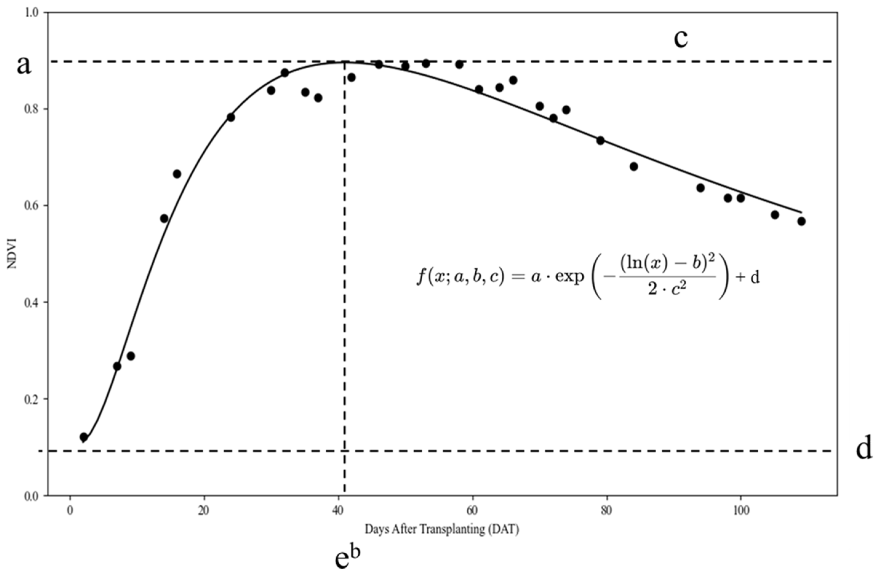
presents the log-normal model fitting parameters (a, b, c, and d) for the NDVI data across various treatment conditions for 2023 and 2024. As nitrogen treatment levels increased, parameter a, representing the peak value of the NDVI curve, generally exhibited an increasing trend. This indicates that higher nitrogen levels contribute to the elevation of maximum NDVI values. Parameter b, which indicated the timing of the NDVI peak, tended to decrease with delayed transplantation dates. This implies that the late transplantation may have caused the NDVI peak to occur slightly earlier. This trend was particularly evident in the 2023 field data, where late transplanting treatments had lower b values than standard transplanting treatments.

Parameter c, representing the spread or distribution of the NDVI curve, varied with the treatment conditions. Higher nitrogen levels typically correspond to higher c values, indicating a broader distribution of the NDVI curve. In contrast, parameter d, representing the baseline or minimum NDVI value, showed minimal variation across treatments, suggesting that the baseline NDVI values remained relatively stable regardless of nitrogen level or transplanting time.

These findings provide valuable insights into how NDVI profiles respond to variations in nitrogen levels and transplantation time. They enhance our understanding of how these factors affect the temporal behavior of VIs. Overall, the R² values for the fitted models were consistently high across different treatments, indicating that the four-parameter log-normal model effectively captured variations in NDVI over time and across treatment conditions. 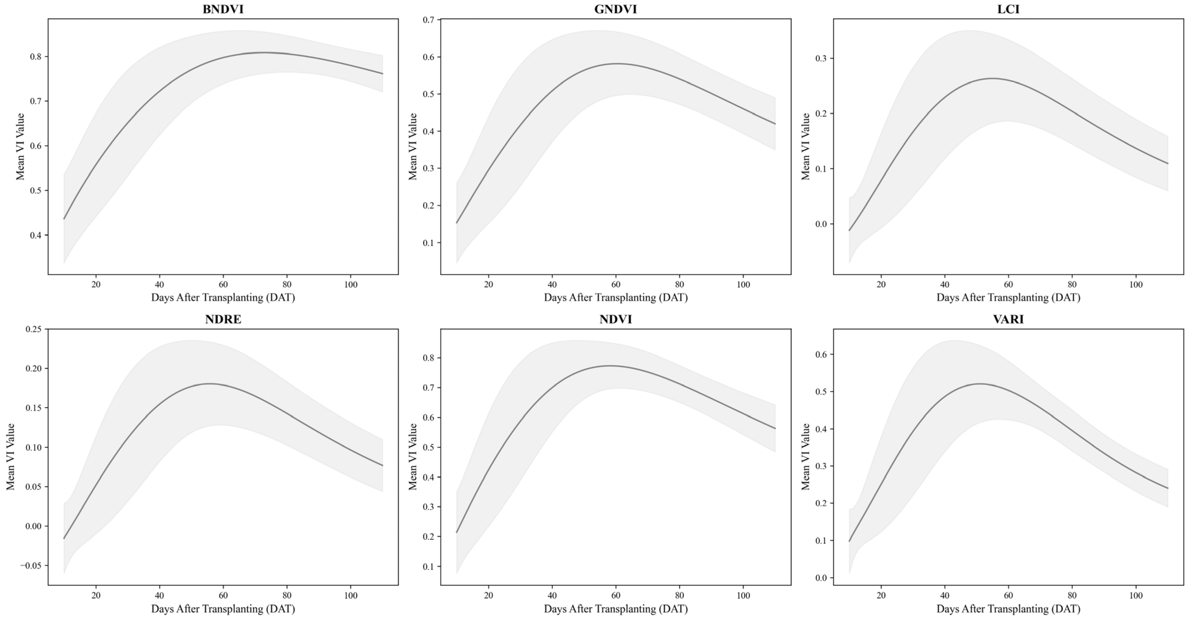Figure 5 shows the deviations in the log-normal curves for each VI. The shaded regions represent the standard deviation around the mean log-normal model fit, visually representing how each index varied across the treatments.

Table 6. Mean, standard deviation, and R² values of parameters for log-normal fitting of VIs across all treatments.

VI	a	b	c	d	R2
BNDVI	0.49 ± 0.22	4.28 ± 0.18	0.94 ± 0.32	0.32 ± 0.21	0.93
GNDVI	0.52 ± 0.16	4.07 ± 0.15	0.69 ± 0.21	0.08 ± 0.13	0.93
LCI	20.39 ± 0.11	3.99 ± 0.16	2.04 ± 0.14	−20.12 ± 0.06	0.89
NDRE	3.77 ± 0.077	4 ± 0.16	1.3 ± 0.15	−3.58 ± 0.04	0.91
NDVI	0.75 ± 0.12	4.03 ± 0.17	0.74 ± 0.21	0.05 ± 0.08	0.95
VARI	67.47 ± 0.12	3.92 ± 0.17	3.83 ± 0.14	−66.91 ± 0.06	0.87

presents the average log-normal model parameters and R² values for each VI. The VIs included the BNDVI, GNDVI, LCI, NDRE, NDVI, and VARI. The consistently high R² values across the indices demonstrated the robustness of the log-normal model in fitting the time-series data. Differences in the parameter values among the VIs highlight their unique responses to environmental and treatment factors, further validating the applicability of this approach for assessing vegetation dynamics.

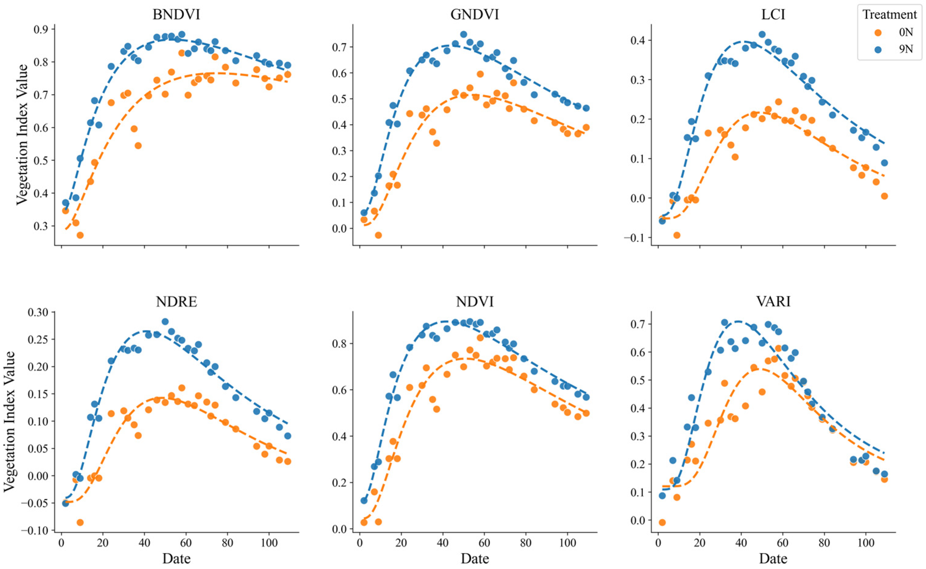
3.4. Comparison of Log-Normal Graphs of VIs by Treatment and Variety

Graphical comparisons were conducted to examine differences among treatments and varieties for each VI fitted as time-series data. Nitrogen application rates influenced the VI curves, with higher nitrogen levels generally resulting in increased values across most indices, indicating improvements in plant health and biomass accumulation. BNDVI, GNDVI, and NDVI exhibited more pronounced peaks and higher values with increasing nitrogen levels.

Furthermore, nitrogen application advanced the timing of VI peaks, suggesting that nitrogen treatments accelerated the time to reach maximum biomass. This pattern, characterized by a rapid peak followed by a decline, reflects the growth dynamics observed under the nitrogen treatment. This highlights the critical role of N in shaping the timing and patterns of plant growth (Figure 6).

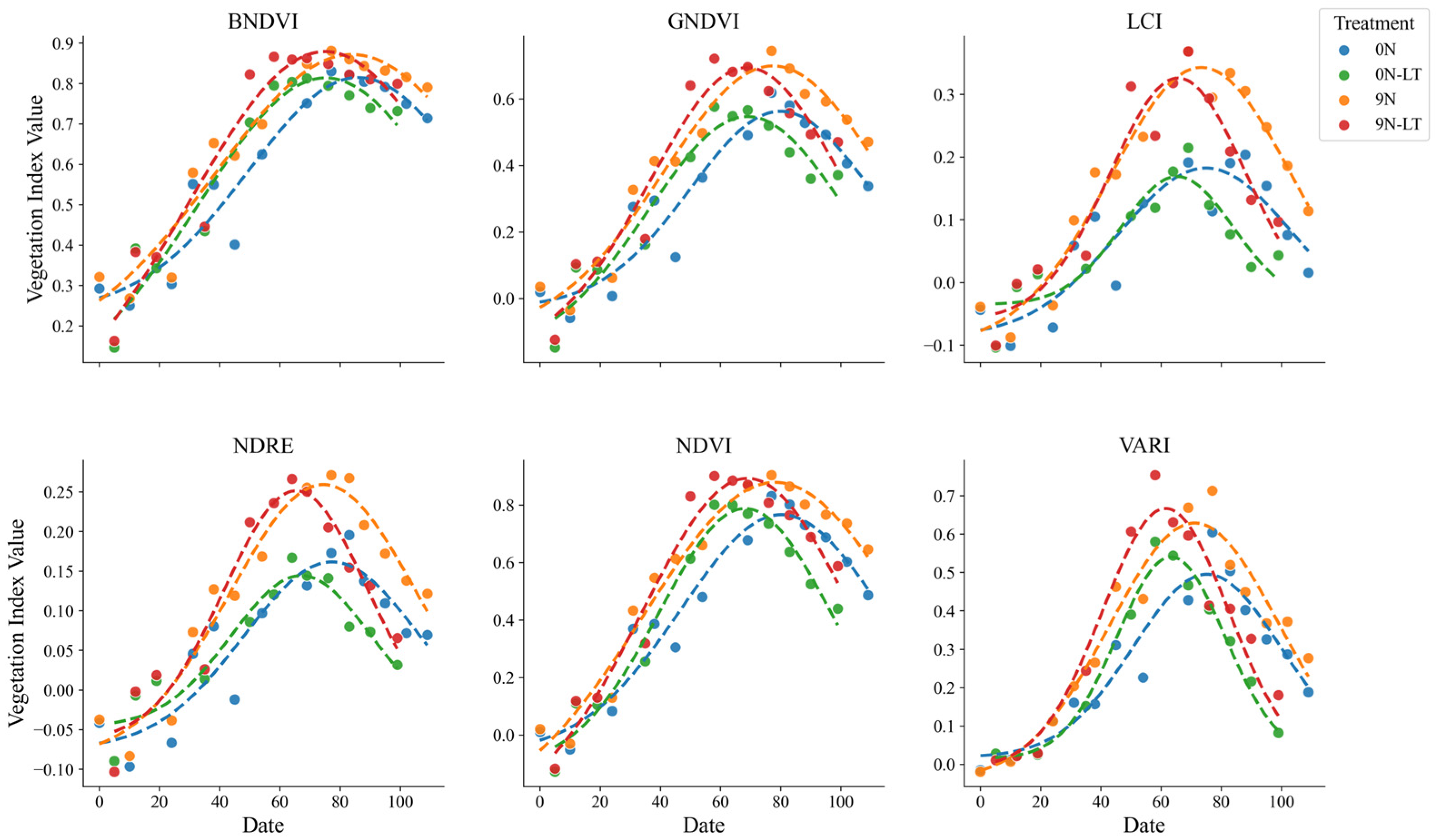
The results were used to analyze the effects of transplanting time and nitrogen treatment on VIs (Figure 7). A longer transplantation time shortened the number of days required to reach the peak VI. Furthermore, a delay of approximately 20 days in transplanting had minimal effect on the peak VI values under nitrogen-treated conditions. However, under nitrogen-untreated conditions, transplanting reduced the overall VI values. This indicates that delayed transplanting considerably affected growth and VIs in the nitrogen-untreated plots.

Minimal differences were observed in the VI patterns under the nitrogen treatment among the four rice varieties (Shindongjin, Dongjin-1, Nampyeong, and Saeilmi), indicating that ecological or phenotypic differences were not evident. This consistency suggests that the log-normal model can be broadly applied to varieties with similar traits, thus providing a reliable framework for analyzing time-series VIs under diverse conditions (Figure 8).

3.5. Effect of VI Patterns on Yield and Yield Components

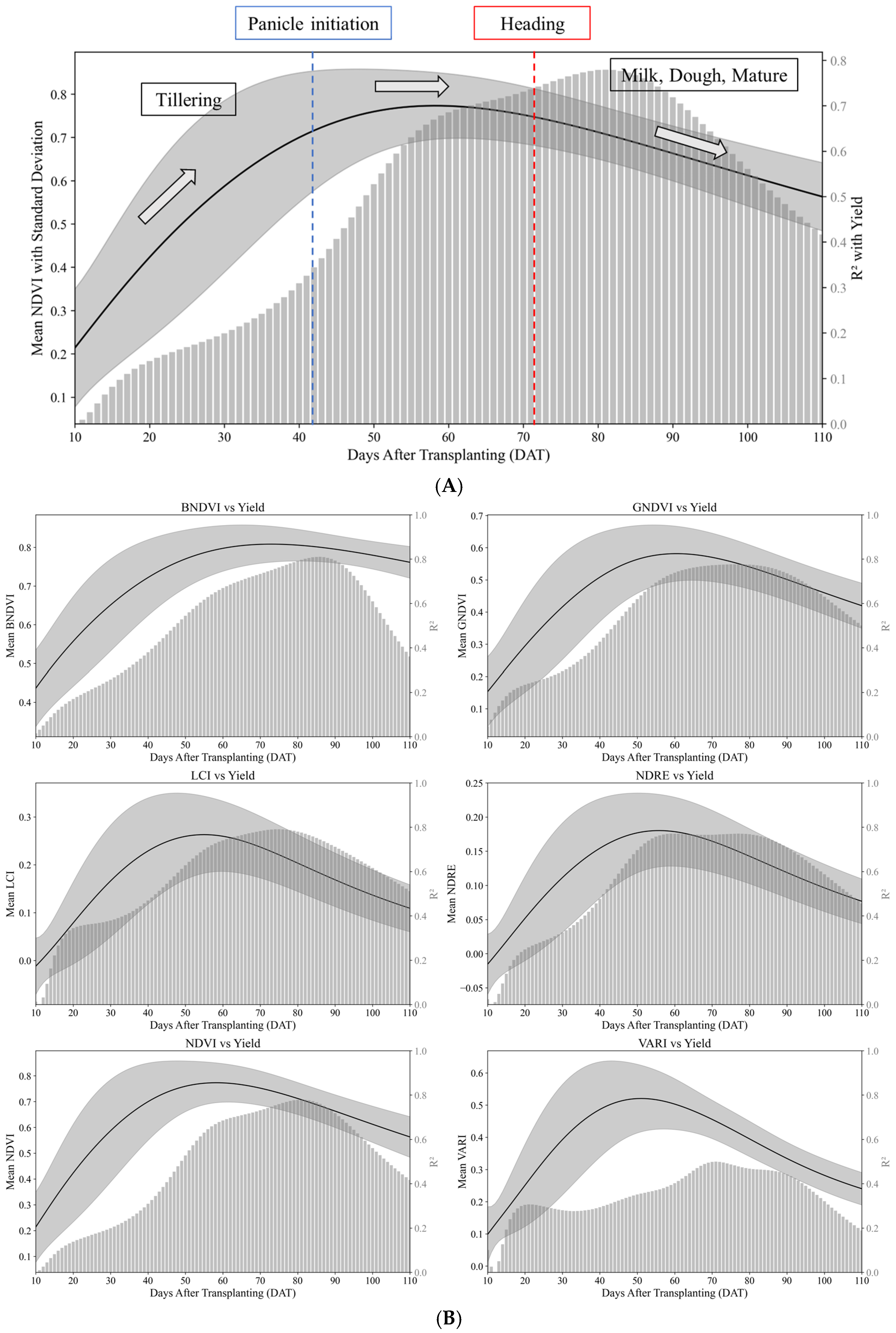
The correlations between the time-series VI values fitted to a log-normal model and the yield are shown in Figure 9. The R² values were consistently higher during the mid-to-late growth stages than during the early tillering stage for all VIs. This indicates that variations in VIs during the early growth phase have a limited influence on yield formation. The gradual increase in R² values during the early growth phase can be attributed to biomass accumulation and its relationship with yield [35].

A detailed analysis focusing on the heading stage revealed that the R² values peaked during or immediately after the heading stage for most VIs. This indicates that the heading stage is closely related to yield formation and that changes in VIs after heading are crucial in yield prediction. Specifically, the increase in R² values after heading can be attributed to the physical canopy of rice leaves being overshadowed by panicles, which affects the VI values [36]. This suggests that the rate and extent of VI decline after heading may be determined by the amount and speed of panicle emergence following nitrogen treatment. These findings highlight that VIs indicate biomass as well as structural changes, such as panicle formation, during the post-heading phase.

The timing of peak R² values varied among VIs, with NDRE showing the earliest and strongest correlation with yield. This suggests that NDRE is particularly sensitive to early growth and nutrient conditions, forming a relationship with yield more rapidly than the other VIs. Conversely, the peak value of VI had less influence on yield than expected, and high standard deviations in VI values did not necessarily correlate with yield differences. The strongest correlations between VIs and yield were observed during the post-peak decline phase, indicating that decreases in VI values during the late growth stages significantly influenced yield-related factors.

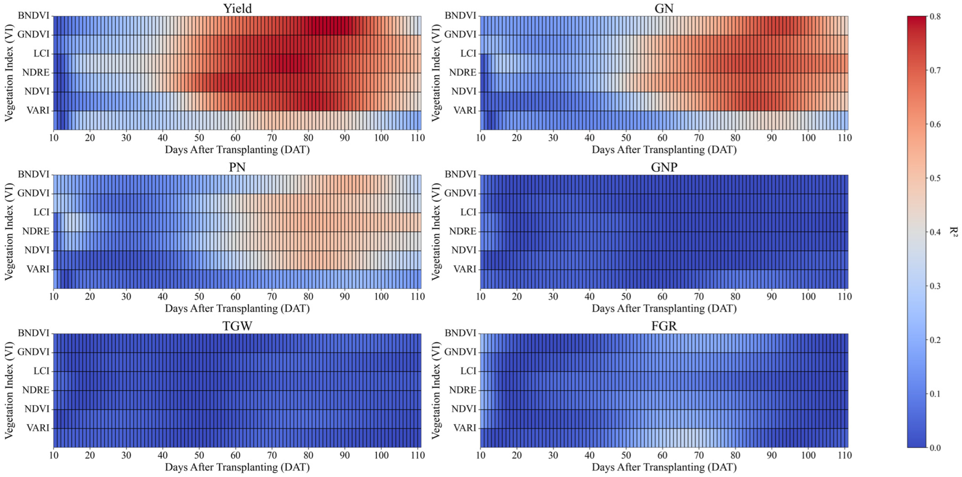
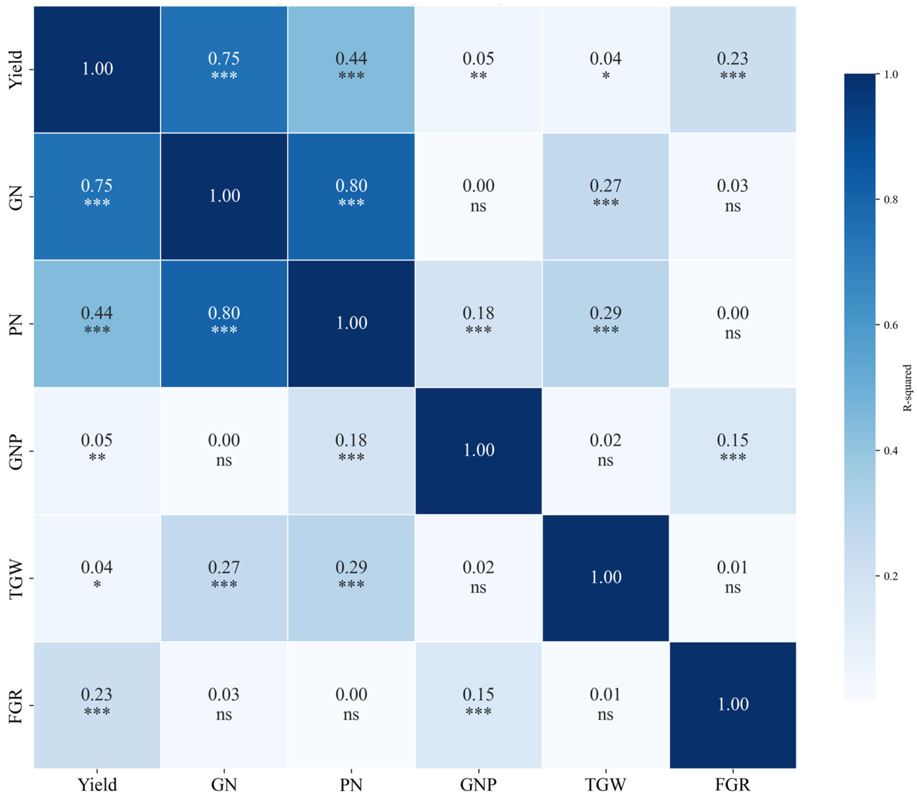
Additionally, Figure 10 shows a heatmap of the R² values for each VI in relation to rice yield, GN, PN, GNP, TGW, and FGR. The overall correlation patterns between the VIs and yield components were similar, with R² values peaking earliest for yield, followed by GN and PN. The magnitude of R² was highest for yield, followed by GN and PN. This indicates that VIs are strongly linked to yield as well as to GN and PN, although the strength of these relationships varies by index. However, GNP, TGW, and FGR were not significantly correlated with yield or major yield components, such as GN and PN, at any growth stage. This suggests that these components have a limited influence on yield variability compared with other yield-related factors.

Table 7. Relationship between yield components and VIs: DAT at peak VI, DAT at maximum R², and coefficient of determination.

	VI	DAT at Peak	DAT at Maximum R2	R2
Yield	BNDVI	73	86	0.8102
	GNDVI	58	77	0.7769
	LCI	53	75	0.7909
	NDRE	53	60	0.7713
	NDVI	59	81	0.7791
	VARI	49	71	0.4993
GN	BNDVI	73	92	0.7370
	GNDVI	58	86	0.7096
	LCI	53	84	0.7273
	NDRE	53	85	0.7034
	NDVI	59	86	0.7280
	VARI	49	90	0.4439
PN	BNDVI	73	91	0.5296
	GNDVI	58	80	0.5117
	LCI	53	82	0.5301
	NDRE	53	82	0.5061
	NDVI	59	82	0.5119
	VARI	49	93	0.2292

summarizes the DAT at which each VI peaked and the maximum R² values for the yield, GN, and PN. It also includes the differences between the DAT at the peak VI value and DAT at the maximum R². R²max typically occurred later than the peak VI values for all VIs, with this lag particularly pronounced for GN and PN. This suggests that vegetation growth patterns influenced GN and PN over an extended period, whereas the relationship between the VIs and yield was relatively immediate.

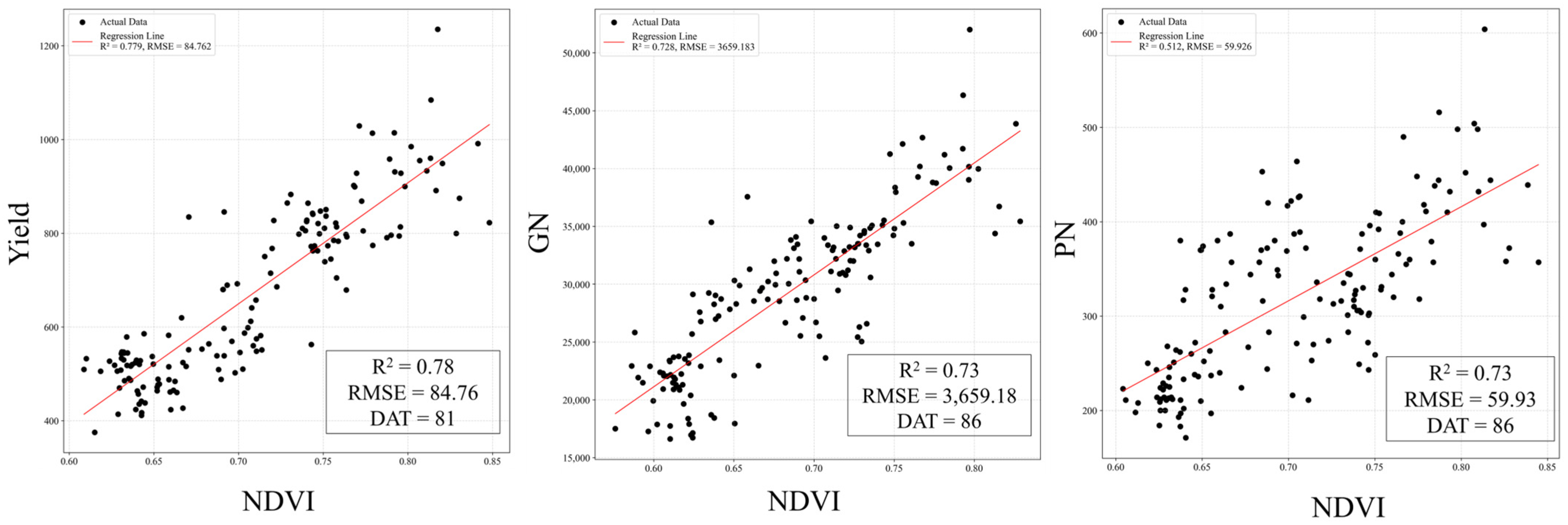
Figure 11 shows the regression analysis of the relationships between the VI values, highlighting the R² and RMSE values. For NDVI, the maximum R² with yield was observed at DAT 81 (R² = 0.78) with an RMSE of 84.76. For GN, the maximum R² was recorded at DAT 86 (R² = 0.73) with an RMSE of 3659.18. For PN, the maximum R² occurred at DAT 82 (R² = 0.51) with an RMSE of 59.95. These results indicate that VI data from specific time points can effectively explain the relationship between yield and its components. However, they also suggest that using VI data from inappropriate time points may lead to errors in yield estimation, underscoring the importance of selecting the correct timing for VI data in predictive analyses.

3.6. Relationship Between Log-Normal Function Parameters and Rice Yield Components

The regression analysis results between the parameters of the log-normal function (a, b, c, d, and a + d) and the rice yield components (yield, GN, PN, GNP, TGW, and FGR) are presented as R² (Figure 12). The combined parameter a + d, which represents the maximum value of the log-normal function, showed the strongest correlation with yield (R² = 0.68), GN (R² = 0.42), and PN (R² = 0.28). Individually, parameter a exhibited moderate correlations with yield (R² = 0.45) and GN (R² = 0.29), whereas the other parameters (b, c, and d) showed relatively weaker correlations. These findings suggest that parameters a and d are key predictors of yield-related traits, particularly when combined.

3.7. Performance Evaluation of Yield Estimation Models

The parameters of four types (a, b, c, and d) derived from individual samples fitted to the model were used as variables for each yield component in the multivariate regression analysis. The analysis employed a linear regression model, PLSR, which effectively handled multicollinearity while objectively identifying the variable characteristics and importance. Additionally, nonlinear machine learning models, such as RFR, GBR, and XGBR, were used to evaluate model performance. R² values were evaluated and determined using the LOOCV method. Regression graphs for the NDVI, models, and each yield component are shown in Figure 13.

Among the VIs, LCI, NDRE, and NDVI consistently demonstrated high predictive performance across all models (

Table 8. Model performance (R²) of yield components for VIs and regression methods.

Yield Components	VI	Models
		PLSR	GBR	RFR	XGBR
Yield	NDVI	0.82	0.74	0.76	0.58
	NDRE	0.71	0.82	0.82	0.84
	VARI	0.5	0.75	0.75	0.76
	LCI	0.72	0.83	0.84	0.84
	GNDVI	0.79	0.64	0.83	0.63
	BNDVI	0.8	0.59	0.61	0.58
GN	NDVI	0.63	0.58	0.73	0.58
	NDRE	0.71	0.77	0.79	0.79
	VARI	0.25	0.63	0.65	0.65
	LCI	0.7	0.83	0.81	0.82
	GNDVI	0.74	0.63	0.79	0.65
	BNDVI	0.39	0.41	0.62	0.56
PN	NDVI	0.49	0.65	0.72	0.74
	NDRE	0.76	0.82	0.81	0.84
	VARI	0.13	0.66	0.7	0.69
	LCI	0.74	0.86	0.85	0.86
	GNDVI	0.72	0.8	0.78	0.8
	BNDVI	0.53	0.68	0.67	0.69
GNP	NDVI	0.12	0.32	0.41	0.35
	NDRE	0.29	0.39	0.43	0.38
	VARI	0.06	0.35	0.35	0.38
	LCI	0.28	0.37	0.41	0.42
	GNDVI	0.16	0.29	0.39	0.26
	BNDVI	0.15	0.24	0.35	0.23
TGW	NDVI	0.11	0.39	0.43	0.39
	NDRE	0.15	0.36	0.44	0.41
	VARI	0.12	0.45	0.51	0.38
	LCI	0.12	0.37	0.38	0.36
	GNDVI	0.14	0.35	0.42	0.32
	BNDVI	0.16	0.25	0.35	0.23
FGR	NDVI	0.43	0.6	0.67	0.58
	NDRE	0.37	0.62	0.62	0.62
	VARI	0.36	0.61	0.57	0.61
	LCI	0.24	0.5	0.49	0.5
	GNDVI	0.32	0.6	0.63	0.55
	BNDVI	0.19	0.66	0.67	0.51

and

Table 9. Model performance (RMSE) of yield components for VIs and regression methods.

Yield Components	VI
		PLSR	XGBR	RFR	GBR
Yield	NDVI	87.16	83.99	83.51	83.38
	NDRE	103.16	77.09	76.28	75.55
	VARI	126.95	87.83	89.18	90.48
	LCI	96.02	80.65	71.21	83.99
	GNDVI	82.75	74.48	75.13	72.69
	BNDVI	80.36	108.99	108.81	109.91
GN	NDVI	5758.87	3684.51	3780.16	3518.25
	NDRE	4102.29	3247.31	3215.17	4443.64
	VARI	6092.48	4990.85	4195.95	4992.32
	LCI	3835.29	2975.59	3042.91	2923.44
	GNDVI	3567.66	3386.00	3353.21	3507.01
	BNDVI	5480.76	4271.84	4292.5	4310.45
PN	NDVI	68.31	46.22	50.68	47.94
	NDRE	42.29	34.75	36.04	36.04
	VARI	79.82	47.37	46.86	49.76
	LCI	43.75	32.07	33.41	33.49
	GNDVI	45.38	39.13	39.65	38.73
	BNDVI	58.29	52.83	49.08	48.75
GNP	NDVI	10.07	9.42	8.41	9.01
	NDRE	9.39	8.74	8.35	8.96
	VARI	10.86	8.8	9.11	8.95
	LCI	9.47	9.08	8.49	9.07
	GNDVI	10.23	9.59	8.79	9.36
	BNDVI	11.97	9.75	8.98	9.74
TGW	NDVI	2.39	2.13	1.92	2.25
	NDRE	2.33	1.92	1.91	2.03
	VARI	2.37	1.99	1.76	1.88
	LCI	2.38	2.03	2.02	2.04
	GNDVI	2.35	2.11	1.96	2.18
	BNDVI	2.73	2.23	2.03	2.2
FGR	NDVI	0.08	0.06	0.06	0.07
	NDRE	0.07	0.06	0.06	0.06
	VARI	0.08	0.06	0.06	0.06
	LCI	0.08	0.07	0.07	0.07
	GNDVI	0.08	0.06	0.06	0.06
	BNDVI	0.1	0.06	0.05	0.06

). On average, LCI and NDRE were better predictors of GN and PN, respectively. LCI showed strong performance in nonlinear models such as RFR, XGBR, and GBR while maintaining a relatively high accuracy in PLSR. NDRE, with its sensitivity to early and mid-growth stages, achieved high predictive performance for GN and PN as well as for yield in XGBR and GBR. Similarly, NDVI exhibited excellent performance in yield prediction, with R² values of 0.82 in PLSR and RFR, comparable to NDRE.

NDVI showed moderate accuracy for GN prediction, with R² values ranging from 0.58 to 0.76, depending on the model, demonstrating its utility in predicting grain production under diverse conditions. The NDVI performed reliably for PN prediction, achieving a peak R² value of 0.74 RFR, indicating its effectiveness in representing panicle density. However, NDVI exhibited relatively lower predictive power for GNP, TGW, and FGR, with R² values below 0.5 for most models, revealing its limitations in capturing meticulous details related to grain quality and weight.

For yield component prediction, GN and PN consistently recorded higher R² values than GNP, TGW, and FGR for all VIs and models, thereby achieving greater predictive accuracy. In contrast, BNDVI showed moderate predictive performance for most yield components but relatively lower accuracy for PN compared to other indices. LCI and NDRE were the most stable and reliable VIs for predicting GN and PN.

Overall, the nonlinear models (XGBR, RFR, and GBR) outperformed PLSR in predicting complex traits such as GN and PN. However, the observed differences in performance among the regression models may stem from both the features of the data and the inherent capabilities of the models themselves. For example, nonlinear models might better capture complex relationships in the data, leading to higher accuracy in predicting traits like GN and PN compared to the linear PLSR model. However, the performance of each model can also be influenced by factors such as the size and quality of the training data, the choice of hyperparameters, and the specific evaluation metrics used. Further investigation is needed to disentangle the effects of data features and model capabilities on the observed performance differences. GNP, TGW, and FGR consistently recorded lower R² values for all VIs, indicating their limited contributions to yield variability. Despite these limitations, NDVI remains a dependable indicator for predicting key yield components, such as GN and PN, reaffirming its significance in yield estimation models.

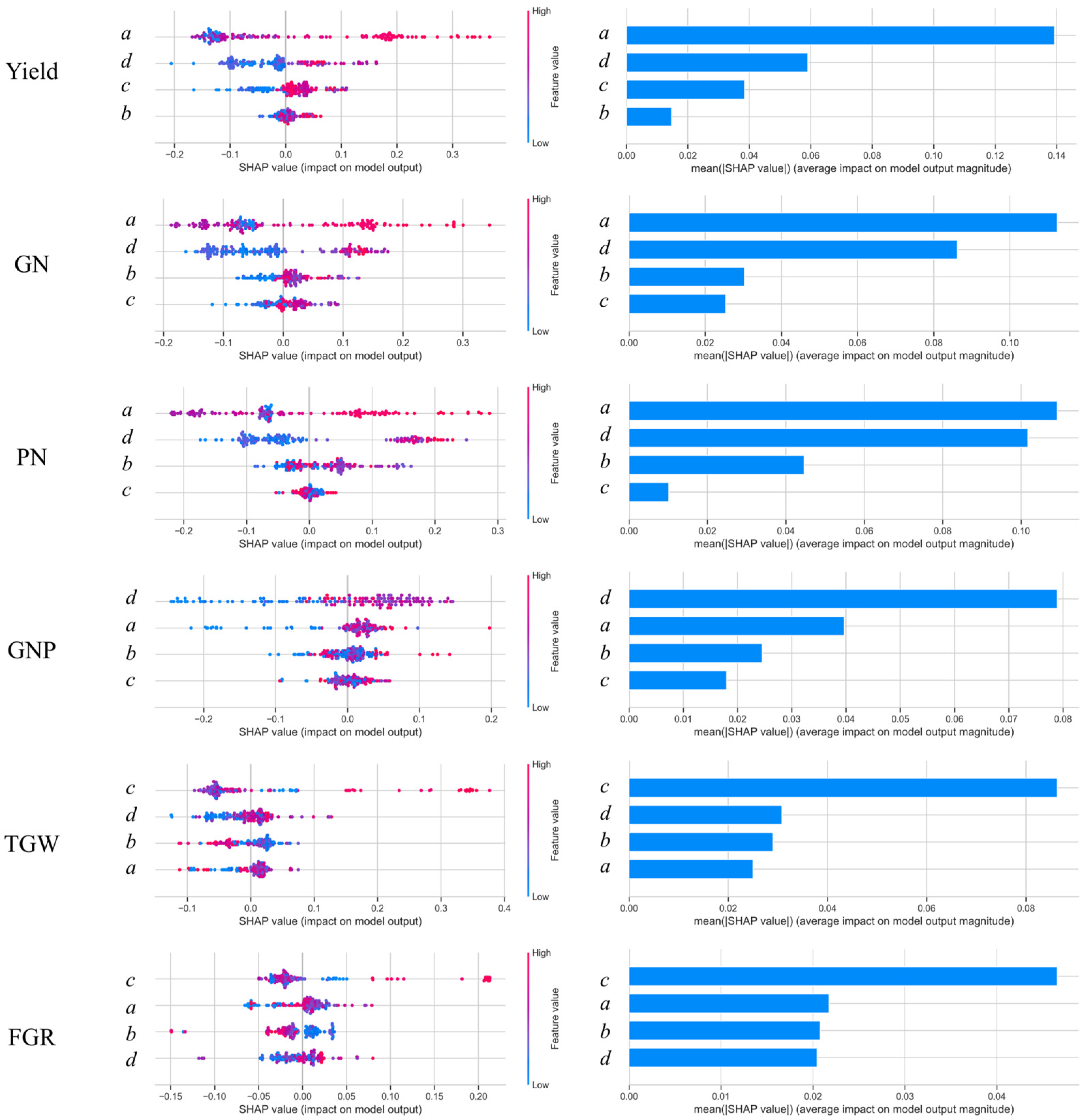
The SHAP value analysis for the NDVI model parameters highlighted the relative importance of four parameters (a, b, c, and d) in predicting the yield components (Figure 14). Parameter a, representing the peak value of the NDVI curve, consistently exhibited the highest contribution to the model outputs across all yield components, reaffirming its strong association with maximum vegetation vigor and yield. Parameter c, indicative of the spread of the curve, also played a notable role, particularly for PN and GN, where broader distributions in the NDVI curves reflected extended growth activity critical for yield formation.

In contrast, parameters b and d showed varying effects depending on the yield component. For GN and PN, b was moderately important, suggesting that the timing of the peak NDVI was relevant for determining reproductive development. However, for secondary yield components, such as GNP and TGW, both b and d had comparatively lower contributions, indicating their reduced influence on finer yield traits.

Overall, the SHAP value analysis underscores the dominant roles of a and c in predicting yield-related traits, underscoring their importance in NDVI-based models. This finding highlights the critical effect of maximum VIs and growth distribution patterns on yield estimation.

4. Discussion

This study successfully modeled time-series VIs, extracted from drone-based multispectral imagery, using a log-normal function and performed machine learning regression analysis to predict rice yield and its components. The results demonstrated that the log-normal function effectively tracked dynamic changes in VIs throughout the rice growth cycle, and key parameters of the function (a, b, c, and d) provided a quantitative explanation of VI curve fluctuations, as influenced by nitrogen treatments and transplanting times. The parameters ‘a’ (maximum value) and ‘c’ (variance) showed strong correlations with yield and yield components, highlighting the critical factors influencing yield formation, particularly during the mid-to-late growth stages. These findings are significant because they offer a novel approach to accurately monitor rice growth and predict yield, thereby contributing to the advancement of precision agriculture.

The higher R² observed between yield and grain number with VIs during the post-heading decline phase compared to the early rapid growth phase indicates that reproductive growth was more active than vegetative growth during this period, suggesting that indices such as NDVI and NDRE are not limited to indicating early growth characteristics such as plant height or leaf area. While these indices generally exhibit correlations among themselves, they displayed distinct characteristics in their relationships with rice yield and yield components, such as the timing of peak R² values and the strength of the correlations. This underscores the potential of these indices to capture the interactions between leaves and panicles during the late growth stages, ultimately reflecting yield formation. These results are consistent with those of previous studies that demonstrated the utility of drone-based VI analyses for rice yield prediction. Studies have reported similar findings highlighting the importance of time-series analyses for monitoring crop growth using UAVs across diverse terrains [37].

Nitrogen application significantly influenced VIs. Higher nitrogen levels increased the maximum VI value (a) and broadened the width of the curve (c), indicating enhanced photosynthetic capacity and extended growth activity owing to increased LAI [15,38]. This effect can be attributed to accelerated growth and development owing to higher average temperatures during the growth period, as suggested by a previous study indicating that high temperatures promote rice growth. Conversely, nitrogen-deficient conditions resulted in a sharp decline in VIs during late growth stages, negatively affecting panicle and grain numbers and consequently reducing yield [34]. These findings reaffirm the critical importance of precise and timely nitrogen application for maintaining consistent growth throughout the rice life cycle. Furthermore, under climate change scenarios, VIs have been proposed as effective tools for monitoring shifts in crop growth cycles [39].

Delayed transplanting advanced the peak of the log-normal function, likely due to accelerated growth driven by high-temperature conditions following late transplanting [33]. However, sufficient nitrogen supply mitigated the negative effects of delayed transplanting, enabling higher initial growth rates and preserving maximum VI levels. This suggests that appropriate nitrogen management can partially mitigate transplantation delays. Conversely, nitrogen deficiency under delayed transplantation conditions resulted in lower maximum VIs, shorter growth periods, and significantly lower yields. Studies integrating drones and satellite imagery have also reported the ability to flexibly track growth differences caused by variations in transplantation time, thereby enhancing prediction accuracy [40].

Machine learning regression analysis showed that NDRE, LCI, and NDVI were highly effective in predicting yield and its components. NDRE, designed to address saturation issues in the late growth stages commonly associated with NDVI, maintained predictive performance throughout the mid-to-late growth stages. This finding is consistent with those of previous studies highlighting the superior late-growth predictive capability of NDRE, especially for tracking nitrogen nutritional status [13,41]. Furthermore, drone-based time-series imagery enables the real-time monitoring of field conditions, such as flooding or lodging, further enhancing the value of machine learning techniques in precision agriculture [42].

The log-normal model-based time-series analysis presented in this study offers a promising approach for predicting yield and quality not only in rice but potentially in other crops, such as wheat, barley, and maize, particularly by focusing on growth conditions around heading or flowering stages. However, this study has some limitations. It did not fully account for various environmental stressors, including detailed weather variations (e.g., extreme temperature events, rainfall intensity), soil properties (e.g., texture, organic matter content), and pest or disease pressures, which can significantly impact crop growth and yield. Future research should involve multi-year and multi-regional experiments to validate and expand the applicability of this approach under diverse environmental conditions [43,44]. Additionally, integrating data from multiple sensors (e.g., hyperspectral, thermal, LiDAR) and incorporating advanced machine learning techniques, such as deep learning, could further enhance prediction accuracy and robustness. Addressing practical challenges, such as the cost of drone operations, data processing requirements, the need for specialized personnel, and weather constraints, will be crucial for the widespread adoption of this technology. This can be achieved through efficient integration with diverse sensors, cloud-based AI platforms, and the development of user-friendly decision support systems for farmers. Economic feasibility studies are also needed to assess the cost-effectiveness of drone-based monitoring for different farming scales and contexts.

5. Conclusions

This study demonstrates a robust and efficient method for estimating rice yield and its components by integrating drone-based, time-series multispectral imagery with log-normal modeling and machine learning. The log-normal function effectively captured the dynamic changes in VIs throughout the rice growth cycle, providing a nuanced understanding of crop development. Critically, the parameters derived from this model, particularly the maximum value (a) and the spread of the curve (c), offered a quantifiable and interpretable link between crop growth patterns and yield-influencing factors such as nitrogen application rates and transplanting timing. Among the tested VIs, NDRE, LCI, and NDVI consistently exhibited superior predictive power across various machine learning models underscoring the importance of capturing not just peak vegetation vigor, but also the rate and timing of senescence—the decline in VIs after the peak—for accurate yield estimation. This is because these late-season changes reflect crucial processes like grain filling. This approach represents a significant advancement by moving beyond simple correlations to quantify the shape of the VI curve and relate it directly to management practices. To further enhance the practical application and robustness of this method, future research should focus on incorporating a wider range of environmental stressors validating the model across diverse geographical locations and multiple growing seasons, exploring the potential of data fusion with other sensor types and combining it with advanced deep learning techniques. Ultimately, this work contributes to the development of more precise, data-driven agricultural practices, supporting improved crop management, resource optimization, and global food security.