Machine Learning-Based Acoustic Analysis of Stingless Bee (Heterotrigona itama) Alarm Signals During Intruder Events

Abstract

Heterotrigona itama, a widely reared stingless bee species, produces highly valued honey. These bees naturally secure their colonies within logs, accessed via a single entrance tube, but remain vulnerable to intruders and predators. Guard bees play a critical role in colony defense, exhibiting the ability to discriminate between nestmates and non-nestmates and employing strategies such as pheromone release, buzzing, hissing, and vibrations to alert and recruit hive mates during intrusions. This study investigated the acoustic signals produced by H. itama guard bees during intrusions to determine their potential for intrusion detection. Using a Jetson Nano equipped with a microphone and camera, guard bee sounds were recorded and labeled. After preprocessing the sound data, Mel Frequency Cepstral Coefficients (MFCCs) were extracted as features, and various dimensionality reduction techniques were explored. Among them, Linear Discriminant Analysis (LDA) demonstrated the best performance in improving class separability. The reduced feature set was used to train both Support Vector Machine (SVM) and K-Nearest Neighbor (KNN) classifiers. KNN outperformed SVM, achieving a Precision of 0.9527, a Recall of 0.9586, and an F1 Score of 0.9556. Additionally, KNN attained an Overall Cross-Validation Accuracy of 95.54% (±0.67%), demonstrating its superior classification performance. These findings confirm that H. itama produces distinct alarm sounds during intrusions, which can be effectively classified using machine learning; thus, demonstrating the feasibility of sound-based intrusion detection as a cost-effective alternative to image-based approaches. Future research should explore real-world implementation under varying environmental conditions and extend the study to other stingless bee species.

1. Introduction

One of the most commonly reared stingless bees in the Brunei Darussalam is Heterotrigona itama (Cockerell, 1918). This stingless bee species is indigenous to Brunei Darussalam and is locally referred to as Lebah kelulut [1]. Despite its diminutive size, the honey produced by H. itama is highly valued, fetching nearly USD 100 per kilogram in the market, significantly exceeding that of Apis mellifera (Linnaeus, 1758) or honey bee, which ranges from USD 20 to USD 40 per kilogram [2]. Research conducted in both urban and forest areas of Penang island, Malaysia, has revealed that H. itama is remarkably abundant, constituting the majority of stingless bee species in the region [3]. In fact, a staggering 90% of stingless bee honey sold in Malaysia is derived from H. itama [2]. This prevalence underscores not only the ecological significance of H. itama but also the substantial financial benefits it offers to local communities.

Natural bee colonies enhance their security by selecting well-protected nesting locations. For example, H. itama typically nests inside logs, with a single entrance through a narrow tube. However, despite this strategic nesting behavior, the bees remain vulnerable to intruder and predator attacks, including those from humans, apes, robber bees, bears, spiders, frogs, geckos, and ants. Female bees or worker bees are commonly assigned as guard bees, with the primary duty of notifying the colony and safeguarding the hive from intruders and predators [4,5]. Guard bees are highly dedicated, maintaining their guarding duties both day and night for multiple days. In addition to their vigilance, they can discriminate between nestmates and non-nest mates, even within the same species, and actively prevent unauthorized entry by attacking intruders and recruiting additional hive members for defense [6]. Their defensive mechanisms involve the use of pheromones, buzzing, hissing sounds, and vibrational signals to alert and mobilize nestmates against threats [7].

Some honey bees release sting alarm pheromones from the mandibular glands to attract other bees to respond to intruders [8], whilst Apis mellifera cypria (Arnold, 1903) (Cyprian honey bee) produces a hissing sound with a dominant frequency of around 6 kHz when confronted with attacks by hornets [9]. Moreover, Kawakita et al. [10] found that the hissing sound of Apis cerana japonica (Radoszkowski, 1877) has unique temporal patterns. Additionally, researchers believe bumble bees produce a hissing sound to signal to the other bumble bees the presence of predators and a buzzing sound as a warning to the predators [11]. Krausa et al. [12] state that the stingless bee species Axestotrigona ferruginea (Walker, 1860) produces thorax vibrations to alert its nestmates of a possible intruder attack. It has been found that the temporal patterns between the repetition of these vibrations are more variable than foraging vibrations, with the airborne component of the vibrations having a very low amplitude. Researchers suspect that more detailed information is encoded in the alarm, such as the nature and severity of the threat [12,13]. This information provides insights into utilizing guard bee sounds to protect a hive by mitigating attacks.

Frequent attacks on honey bee colonies from predators not only weaken the hive but also reduce honey production and may ultimately lead to colony collapse. Therefore, beekeepers have taken various measures to protect their hives. In support of these efforts, researchers have been exploring different methods to safeguard beehives from threats, with a particular focus on detecting varroa mites. Numerous computer vision-based techniques have been proposed, with some leveraging deep learning models such as YOLOv5, Single Shot Multibox Detector (SSD), Deep Support Vector Data Description (Deep SVDD) [14], ResNet50, and Vision Transformers [15]. Voudiotis et al. [16] utilized faster R-CNN to develop an electronic bee-monitoring system to combat the threat from varroa mite. Furthermore, vibration analysis with accelerometers has been used to detect varroa mites by distinguishing their unique movement patterns on brood combs [17]. Other researchers have also used different sensors, such as a Bee-Nose gas sensor in reference [18], to estimate mite populations via air quality [16].

However, varroa mites are not the only threat to honey bee colony health, although they have received the most research focus. In response to this, Torky et al. [19] proposed a method to detect not only varroa mites but also hive beetles, ant infestations, and missing queens using the MobileNet model. Ntawuzumunsi et al. [20] utilized a digital camera to detect bee predators, recognizing birds or moths entering the hive.

Beyond computer vision approaches, Rosli et al. [21] attached a force-sensitive resistor to the hive surface to detect the presence of bee predators. However, this approach produced a high number of false positives, as it considered all surface impacts as threats. Alternatively, Bohušík et al. [22] proposed using motion sensors to detect the movement of wild animals and humans, which is also effective in identifying hive theft by humans.

While various sensor-based approaches have been explored, researchers have yet to extensively utilize the natural alarm signals produced by bees in response to threats and predators. Developing a system that leverages these acoustic signals can significantly reduce both sensor costs and processing power, especially compared to image-based approaches. Using the acoustic features of alarm sounds offers a more efficient solution. Therefore, this research focused on investigating the sounds produced by H. itama during intrusions, with the aim of classifying these sounds using shallow learning algorithms to identify potential threats. One of the main limitations in bioacoustics data analysis or classification is lack of acoustic data. Therefore, this research also focused on collecting acoustic data of H. itama by developing suitable hardware and software components.

Sound datasets are often high-dimensional, making dimensionality reduction essential for effective analysis. By reducing the dataset dimensions, irrelevant, noisy, and redundant patterns are eliminated, thereby decreasing the computational resources such as time, memory, and processing power required to handle the data. Dimensionality reduction also improves accuracy by minimizing overfitting and facilitates easier examination and visualization of the data [23].

The objective of this study was to investigate the alarm sounds produced by H. itama in response to intrusions and develop a classification model using shallow learning algorithms to identify potential threats. Due to limited availability of bioacoustics data, a data-collection system was designed for data collection, with the features extracted from the collected data reduced via dimensionality reduction techniques before classification in order to enhance the classification accuracy as well as improve the computational efficiency.

2. Materials and Methods

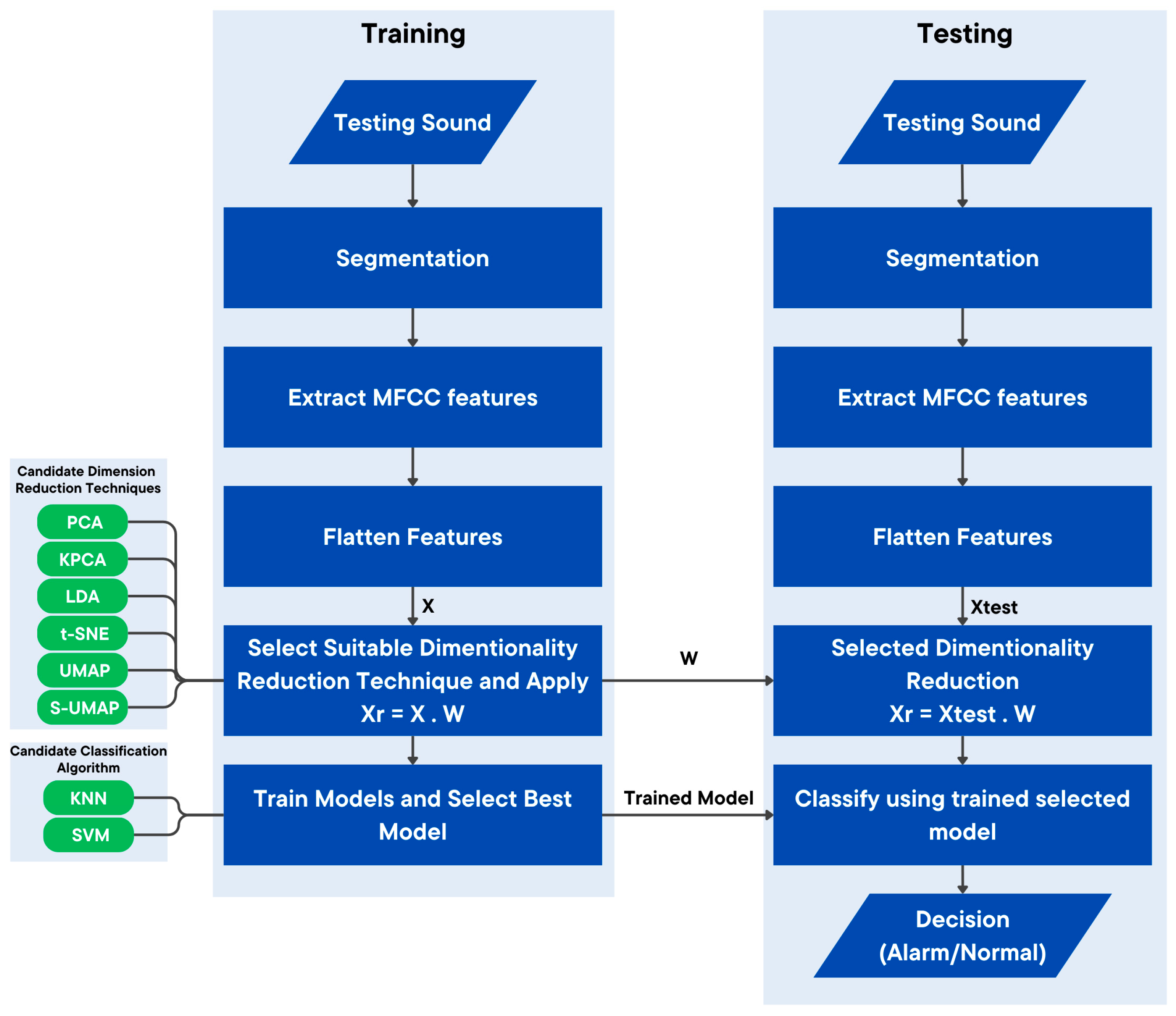
A structured methodology, as illustrated in Figure 1, was used to identify the sounds produced by H. itama bees during intrusion events. A data acquisition system was developed to reliably capture high-quality audio recordings from bee colonies by integrating hardware and software components. A systematic data collection procedure was adopted to capture audio from colonies under both normal and simulated intrusion scenarios, ensuring that the collected audio data were a real representative of the bees’ natural behaviors whilst minimizing disruption to the colonies. Controlled experiments were conducted to mimic intrusion events. The collected data were then pre-processed by labeling, segmenting, and cleaning the raw data, thereby transforming the raw audio recordings into a structured and properly labeled format that is suitable for the subsequent feature extraction and classification tasks. Relevant features were extracted from the processed data, with dimensionality reduction techniques used to reduce the dimension of the features to reduce complexity whilst preserving pertinent information. The reduced feature set was subsequently fed into machine learning models for training. The trained machine learning models allow for the detection of alarm behaviors triggered by intrusions.

2.1. System Development for Data Collection

A data acquisition system was developed to capture the alarm sounds produced by H. itama bees during intruder events, with audio recording serving as the primary data collection method and video footage serving an auxiliary role, providing a visual context to assist in accurate event labeling. The system integrates both hardware and software components, ensuring reliable and high-quality data collection of the bee hives.

2.1.1. Hardware

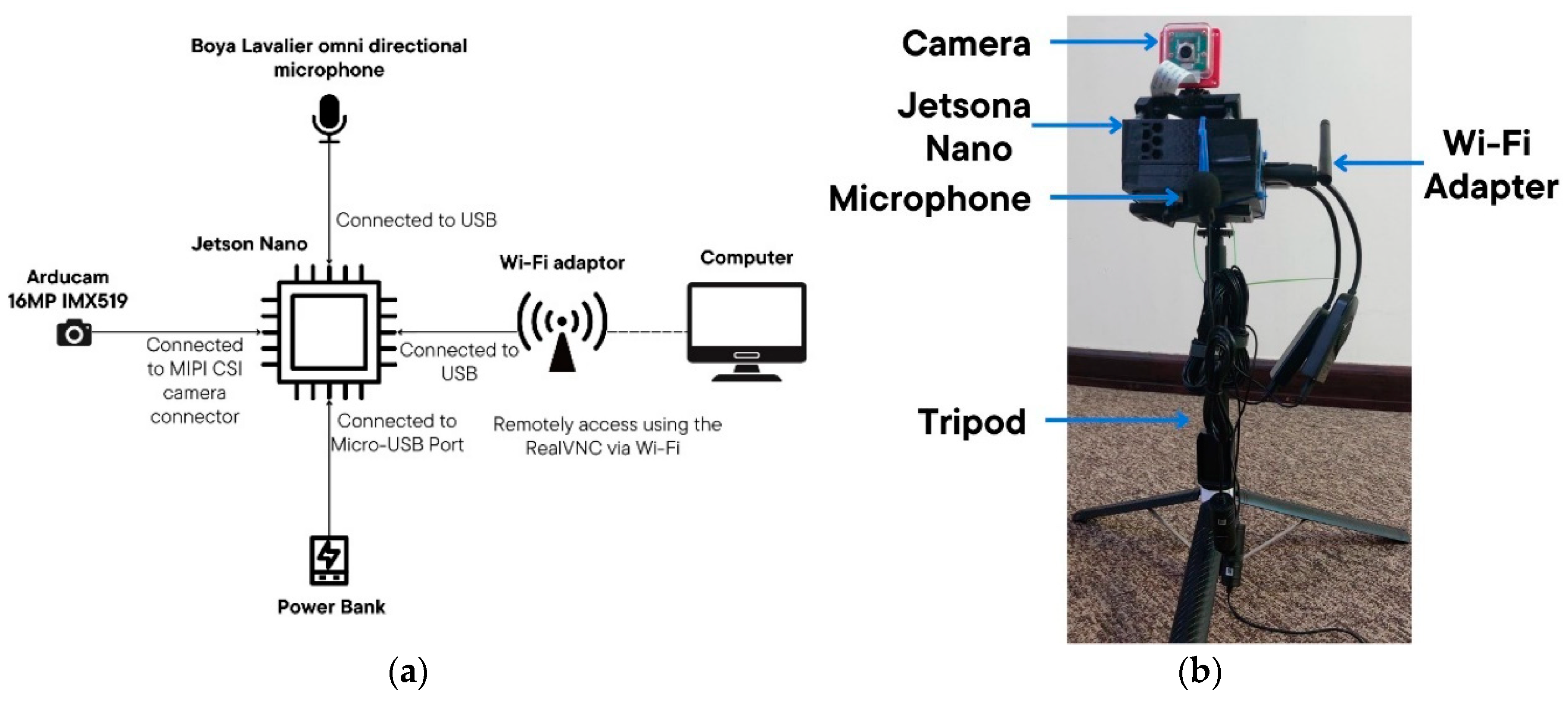
The data acquisition system was built around an NVIDIA Jetson Nano, which serves as the central processing hub for managing and storing data. It was developed to operate remotely near the hive, thereby ensuring high-quality audio recordings whilst causing minimal disturbance to the bees. The main components of the setup are as follows:

• NVIDIA Jetson Nano: Runs the software for both audio and video recording, ensuring synchronized capture of both data streams. The Jetson Nano also enables remote access and control of the system, allowing researchers to monitor and adjust settings without direct interaction with the hive.
• Microphone (Boya Lavalier BY-M1): Positioned close to the hive entrance using its 2 m cable to capture bee sounds with minimal interference.
• Camera (Arducam 16MP Autofocus Camera Module, IMX519): Focused on the hive entrance through the software to record visual data in sync with audio recordings.
• Power Source (20,000 mAh Power Bank): Provides continuous power for extended data collection sessions.
• Wi-Fi Adapter: Enable remote access to Jetson Nano via RealVNC.
• Tripod and adjustable mount for camera.

Figure 2 illustrates the hardware setup, with Figure 2a showing the schematic of the connections and Figure 2b depicting the assembled system. Each component contributes to a reliable, minimally invasive setup for capturing bee audio and video data necessary for subsequent analysis.

2.1.2. Software

A custom Python-based software application was developed to manage the audio and video recording processes, with audio as the primary data source and video supporting data labeling. The software was optimized for real-time data acquisition, remote control, and efficient data management, ensuring smooth operation in field settings. The key features and functionalities of the software include the following:

• Dual-Process Recording of Audio and Video: The software simultaneously captures audio and video as separate processes. This setup ensures synchronized recordings while maintaining independent data files for each stream. By prioritizing audio quality, the software supports the primary objective of capturing bee sounds in high resolution, while the video serves as a reference for labeling intrusion events.
• Remote Access and User Control: To allow for non-intrusive system monitoring, the software was integrated with RealVNC, enabling researchers to remotely access and control the system over Wi-Fi. Through the RealVNC interface, users can adjust the camera’s focus, start and stop recording, and monitor the camera’s view in real time to verify alignment and positioning. This feature minimizes disturbance to the bees and allows for adjustments to be made without a direct interaction with the hive.
• Automated File Management: The software organizes recorded files by segmenting each recording session into 10 min intervals. Each audio or video file is automatically saved with a timestamped filename, simplifying data retrieval and ensuring accurate documentation of events over time. Audio files are saved in the WAV format, an uncompressed, lossless file format that preserves sound quality, essential for analyzing acoustic patterns. The recording is set at a 48 kHz sampling rate and a 32-bit float bit depth, thereby optimizing the audio resolution and ensuring relevant sound frequencies are fully captured by the system.
• Data Handling and Storage: Each recording session is organized by date and time, with the software systematically organizing recording sessions in structured directories. This allows for quick and easy access to specific data points during analysis.
• Error Handling and Recovery: The software also incorporates basic error-handling protocols to maintain data integrity. In the event of connectivity issues or power fluctuations, it is capable of recovering audio recordings without data loss, thereby ensuring continuous data collection.
• Support for Post-Processing: The software integrates with external libraries, including Librosa for audio analysis and OpenCV for video analysis.

Overall, the software setup is designed to meet the needs of quality data collection: audio data to capture the acoustic characteristics of the bees and video data to aid in the labeling of data. Through automated file management and remote access, the software enables an efficient and reliable operation, ensuring prolonged data collection in outdoor settings with minimal disturbances to the bees.

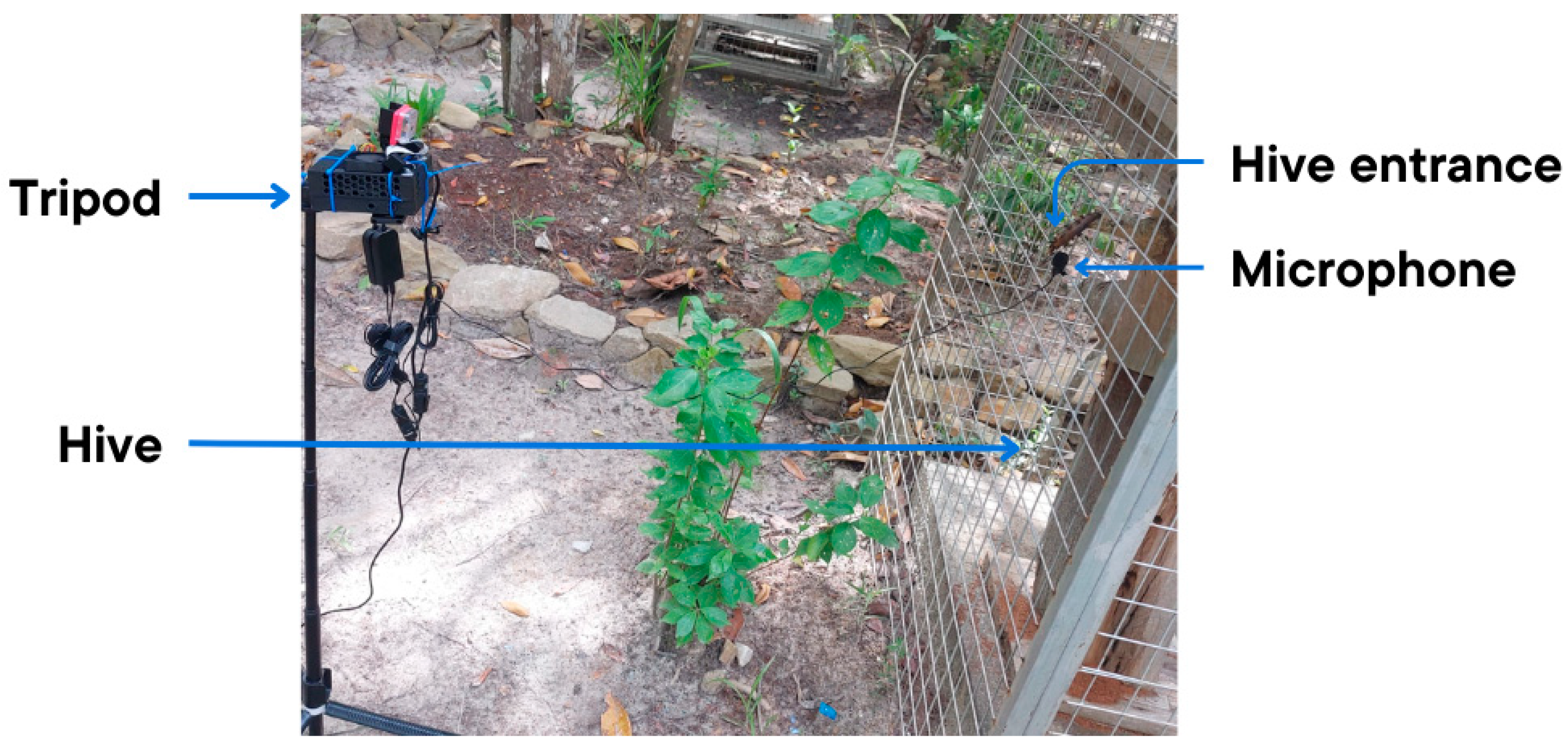
2.1.3. Setup and Calibration

The system was positioned near the hive entrance, as illustrated in Figure 3; a microphone was placed close to the hive entrance to allow for recordings of subtle sounds associated with bee activity, and another microphone was placed alongside the camera. This strategic microphone placement allows for accurate sound capture by isolating bee-generated sounds from other environmental noise. A camera captured a clear view of the hive entrance in order to provide a visual context for each recording. This visual information is required for the accurate labeling of events, with the video data offering a direct reference for identifying the timing and nature of intrusion scenarios.

The system was calibrated prior to data collection: microphone sensitivity was tested to confirm its ability to detect even faint sounds from the hive, with audio gain settings adjusted accordingly for optimal sound capture. Simultaneously, the camera was aligned to capture an unobstructed view of the hive entrance. Beyond the initial calibration, the system enables real-time remote monitoring of both audio and video recordings, thereby allowing researchers to make real-time adjustments as required. This ensures that both audio and video recordings would meet quality standards with minimal disturbances to the bees.

2.2. Data Collection Procedure

Data collection was conducted on three domesticated H. itama colonies at the Universiti Brunei Darussalam Botanical Research Centre from June 2024 to September 2024. The experiments were carried out on non-rainy days at different times of the day, ranging from as early as 7:30 AM to as late as 5:30 PM. The Botanical Research Centre, a six-hectare botanic garden in Brunei Darussalam, houses over 500 species of tropical plants, many of which are native to Brunei Darussalam and Borneo. The colonies were placed in a shaded outdoor environment, surrounded by dense vegetation that provides a natural foraging habitat. The temperature in the area typically ranges from 23 °C to 33 °C, with relative humidity levels of above 80%. The hives were positioned on elevated stands to prevent ground-level disturbances and reduce exposure to potential predators. The colonies used in this study were actively producing honey, which was periodically harvested, ensuring that the colonies were strong and healthy. This garden is also home to various reared stingless bee species, including Heterotrigona itama, Geniotrigona thoracica (Smith, 1857), and Lepidotrigona binghami (Schwarz, 1939).

Audio and video recordings were captured for both normal hive behavior and carefully simulated intrusions. The data collection process began by setting up the system near the hive, as shown in Figure 3. The software was then initiated, storing 10 min long audio and video recordings continuously on the hard drive of the system. To allow the bees to acclimate to the system, a waiting period of 30 min was observed before any disturbances were introduced.

To simulate an intrusion event, a thin stick was gently inserted into the hive entrance, mimicking an intruder’s presence without causing any real harm to the bees; a similar approach was adopted by Djoko et al. [24]. After each artificial intrusion, a 20 min waiting period was maintained to allow the bees settle before any further actions. This process was repeated no more than three times per hive per day to minimize any advertent impact on the well-being of the bees. The same procedure was carried out for all three hives at different times (non-parallel) to improve the precision of labeling. Since the hives were located close to one another, staggering the data collection ensured that recorded behaviors were accurately attributed to the correct hive without cross-interference. By following this approach, high-quality data representing both normal and alarm behaviors were gathered, creating a rich dataset for analyzing the acoustic patterns associated with hive defense.

2.3. Data Processing

The recorded audio files were manually labeled by reviewing the corresponding video footage, with each labeled event stored in a structured CSV file. Details, including the file name, start and end times of the intrusion, intrusion type, and hive identifier, were kept as illustrated in

Table 1. Sample rows from the labeled dataset.

File	Start	End	Hive
20240727152627103.wav	7:32	7:41	Hive A
20240727152627106.wav	5:48	6:00	Hive A
20240804125447102.wav	4:31	4:41	Hive B
20240804125447105.wav	3:22	3:33	Hive B
20240914113641117.wav	1:58	2:19	Hive C
20240914113641119.wav	6:27	6:45	Hive C

. Consequently, this labeling process yielded a dataset consisting of 32 different intrusion simulations.

2.3.1. Data Pre-Processing

Using Python (version 3.11.11), the audio files were pre-processed with the aid of the Librosa (version 0.10.2) and Pandas(version 2.2.2) libraries. Initially, the CSV file was loaded to extract relevant segments of audio data based on the labeled start and end times of each intrusion event. These extracted segments were then divided into 1 s intervals, with each interval labeled as either “Alarm” (for intrusion-related sounds) or “Normal” (for baseline behavior).

To ensure focus on the intrusion event, audio recorded 5 min before and 5 min after each labeled intrusion was excluded from further analysis. The remaining audio, not associated with intrusion events, was labeled as “Normal”. The distribution of data points for each label across the three hives is shown in

Table 2. Number of data points per label.

Label	Hive A	Hive B	Hive C	Total
Alarm	164	118	37	319
Normal	1415	1731	246	3392

.

2.3.2. Balancing the Dataset

Due to the natural imbalance in the dataset, with a significantly higher amount of “Normal” data compared to “Alarm” data, steps were taken to ensure that both classes were evenly represented. Imbalanced data can adversely affect the performance of shallow learning algorithms, leading to biased results. To address this, oversampling was applied to the “Alarm” class, and the “Normal” class was randomly under-sampled.

For oversampling, a windowing technique with overlapping windows was applied to the “Alarm” data using a 0.2 s overlap between 1 s segments [25] as depicted in Figure 4. This approach increased the number of positive samples in the “Alarm” class, resulting in a total of 1595 samples. To match this, the “Normal” class was randomly under-sampled to 1595 samples, bringing the final dataset size to 3190 samples.

Balancing the dataset in this way mitigates the negative effects of data imbalance, especially for algorithms like Linear Discriminant Analysis (LDA), where balanced data improves classification performance [26]. This approach ensures that both “Alarm” and “Normal” sounds are equally represented, creating a robust dataset for training and testing.

2.3.3. Analysis of the Dataset

Both alarm and normal sounds were visualized separately using time-series waveforms and spectrograms. Previous research, albeit on honey bees, has shown that they produce alarm sounds within a specific frequency range, highlighting the need for frequency domain analysis. The Short-Time Fourier Transform (STFT) was used for this purpose. Frequency bins were analyzed to identify variations in magnitude between alarm and normal sounds. The dissimilarity $P$ between alarm and normal sounds was calculated using the Difference Between Median (DBM) and Overall Visible Spread (OVS) [27]:

$$P={\displaystyle \frac{DBM}{OVS}}\times 100$$

(1)

2.4. Feature Extraction and Classification

Several spectral feature extraction techniques, including Fast Fourier Transform (FFT), STFT, Constant-Q Transform (CQT), Chroma, and Spectral Contrast, were considered for transforming time-domain audio into frequency-domain representations. While these methods provide valuable spectral representations, they do not capture perceptual frequency patterns essential for distinguishing acoustic signals.

To address this, cepstral feature extraction was investigated. Whilst direct research on H. itama acoustic patterns is nonexistent, studies on honey bees have shown that they emit distinct sounds across a wide frequency spectrum, often dominated by frequencies around 6 kHz [9]. Given the similarities in behavioral and defensive mechanisms among social bee species, it is reasonable to infer that H. itama may also exhibit comparable acoustic patterns, providing the justification for using cepstral features to capture its acoustic characteristics. Among the different cepstral feature extraction techniques, Mel-frequency cepstral coefficients (MFCCs) were selected for their performance in capturing important frequency-related features specific to bee sounds [28]. MFCCs are widely used in bioacoustics audio processing because they mimic human auditory perception [29].

The MFCC extraction process generated a total of 1222 features, which required further dimensionality reduction to streamline processing and reduce computational overhead. The feature extraction and reduction processes are illustrated in Figure 5.

2.4.1. Techniques for Dimensionality Reduction of Features

To make the dataset more manageable, computationally efficient, and reduce redundancy and noise (to avoid the curse of dimensionality), five dimensionality reduction techniques were evaluated: LDA, Principal Component Analysis (PCA), Kernel Principal Component Analysis (KPCA), t-Distributed Stochastic Neighbor Embedding (t-SNE), and Uniform Manifold Approximation and Projection (UMAP). These methods were assessed by projecting features into a 3D space to visualize clustering and the separation between the two sound classes: alarm and normal. For implementation, Scikit-learn was used for PCA, KPCA, and t-SNE [30], while UMAP-learn was employed for UMAP and Supervised-UMAP (S-UMAP) [31]. Notably, the same UMAP-learn function was utilized for both UMAP and S-UMAP simply by changing selected parameters to adapt to supervised learning.

Table 3. Methods utilized for dimensionality reduction.

DR algorithm	Used Function	Library
PCA	sklearn.decomposition.PCA	Scikit-learn
KPCA	sklearn.decomposition.KernelPCA	Scikit-learn
t-SNE	sklearn.manifold.TSNE	Scikit-learn
UMAP	umap.UMAP	UMAP-learn
S-UMAP	umap.UMAP	UMAP-learn

provides an overview of the libraries and functions used for each technique.

The default LDA function in Scikit-learn provides only N−1 dimensions, with N representing the number of classes in the dataset. Consequently, for a dataset with two classes, the LDA function reduces the data to a single dimension only, limiting its ability to capture more complex feature representations. To allow for greater flexibility in retaining dimensions and enable comparisons with other techniques, the default LDA implementation requires modification. An LDA algorithm was developed using Singular Value Decomposition (SVD) to allow for greater flexibility in determining the number of retained dimensions and, hence, enhancing its utility for comparative analysis with other dimensionality reduction techniques.

The LDA process begins with representing the dataset as a feature matrix $X \in R^{N\times M}$, where N is the number of samples (3190) and M is number of features (1222):

$$X=\left[\begin{array}{ccc}{x}_{11}& \cdots & x_{1M}\\ ⋮& \ddots & ⋮\\ x_{N1}& \cdots & x_{NM}\end{array}\right]$$

(2)

For each class c, a mean vector ${\mu }_{c } \in R^M$ is calculated, along with an overall mean vector $\mu \in R^M$, as follows:

$${\mu }_c={\displaystyle \frac{1}{N_c}}\sum _{i \in class c}{x}_i$$

(3)

$$\mu ={\displaystyle \frac{1}{N}}\sum _{i=1}^N{x}_i$$

(4)

where $N_c$ represents the number of samples in class c (1595 for both classes). Using these mean vectors, the Within-Class Scatter Matrix $S_w \in R^{M\times M}$ and Between-Class Scatter Matrix $S_b \in R^{M\times M}$ are calculated to capture the variance within and between classes:

$$S_w=\sum _{i \in class c}\sum _{i \in class c}(x_i-{\mu }_c){(x_i-{\mu }_c)}^T$$

(5)

$$S_b=\sum _{i \in class c}{N}_c(x_i-\mu ){(x_i-\mu )}^T$$

(6)

The matrix $S \in R^{M\times M}$ is then derived by calculating the product of Within-Class and Between-Class Scatter matrices:

$$A={S_w}^{-1}{S}_b$$

(7)

SVD on matrix A decomposes it as follows:

$$A=U.\mathsf{\Sigma }{.V}^T$$

(8)

where $U \in R^{M\times M}$ and $V \in R^{M\times M}$ are orthogonal matrices, and $\mathsf{\Sigma } \in R^{M\times M}$ is a diagonal matrix containing the singular values of matrix A. The columns of $U$ corresponding to the largest singular values are selected as the basis vectors for the transformation matrix W, which maximizes the separation between classes. The transformation matrix W is, thus, obtained as follows:

$$W=U[:,1:F]$$

(9)

where $F\le M$ is the expected number of features after dimensionality reduction. Finally, the original feature matrix X is projected onto this new reduced space using W, resulting in the transformed feature set $X_{lda} \in R^{M\times F}$:

$$X_{lda}=X.W$$

(10)

The result of this transformation is a reduced dimensional feature set that effectively separates the alarm and normal classes, as illustrated in Figure 5. This dimensionality reduction not only simplifies the dataset but also enhances the ability to distinguish between classes, setting up a robust foundation for classification.

2.4.2. Classification Model

After selecting the optimal dimensionality reduction method, it was applied to reduce the dimensionality of the extracted MFCC features to give a more manageable feature set for classification. This reduced feature set was then used to train two shallow learning algorithms K-Nearest Neighbors (KNNs) and Support Vector Machine (SVM)—to classify the bees’ sounds into alarm and normal categories [32].

Given the relatively limited size of the dataset, a 5-fold cross-validation technique was employed to ensure robust model evaluation. Cross-validation helps mitigate the risk of overfitting by splitting the data into five subsets, allowing each subset to be used as a validation set in turn while the remaining data are used for training. This approach provides a more reliable assessment of model performance across all samples.

KNN and SVM were selected based on their effectiveness in similar acoustic classification tasks, as highlighted in reference [28], and they demonstrated a high classification accuracy relative to other models like Linear Regression, Random Forest, and ensemble techniques. KNN is known for its simplicity and effectiveness in smaller datasets, while SVM is well-suited for binary classification with clear class boundaries, making them ideal choices for this study. The KNN algorithm is a supervised machine learning algorithm used for classification, which makes predictions based on the classes of the K-Nearest Neighbors. Here, K is the number of neighbors selected by the user initially to make the decision. KNN is robust to noise and works well with a large amount of training data, although its computation time can be high. On the other hand, SVM is also a supervised learning model that primarily focuses on binary classification. The main objective of SVM is to determine the optimal classification hyperplane (decision boundary) in an n-dimensional space, maximizing the margin between the classes [33].

The trained KNN and SVM models were evaluated based on their ability to accurately distinguish between the alarm and normal sounds produced by H. itama bees. Both models were optimized through hyperparameter tuning and validated using a 5-fold cross-validation technique to ensure consistent and reliable performance across the dataset. In the case of KNN, the optimal number of neighbors was determined experimentally, whilst for SVM, the selection of the most effective feature set and kernel configuration was important for performance optimization. The choice of these models, supported by findings in the literature, provides a focused approach to classifying bee alarm sounds with high accuracy.

2.4.3. Performance Metrics

Several key metrics, Macro Precision, Macro Recall, Macro Accuracy, and Macro F1 Score, were used to assess the effectiveness of each model in distinguishing between alarm and normal sounds. Applied across the 5-fold cross-validation process via averaging, the macro-averaged metrics provide a robust and balanced evaluation of the models’ performance. In the 5-fold cross-validation process (k = 5), each metric was calculated within each fold, with the final macro-averaged score obtained by averaging the results across the 5 folds.

Macro Precision measures the ability of the model to identify alarm sounds among all instances predicted as alarms; it is calculated as the proportion of true positives out of all positive predictions made and averaged across the 5 folds.

$$Macro Precision(P)={\displaystyle \frac{{\sum }_{i=1}^k{TP}_i}{{\sum }_{i=1}^k({TP}_i+{FP}_i)}}$$

(11)

where ${TP}_i$ and ${FP}_i$ represent the true and false positives in the ith fold, respectively. On the other hand, Macro Recall measures the sensitivity of the model in identifying all actual alarm instances across all folds. It is calculated as the proportion of true positives out of all actual positive instances:

$$Macro Recall(R)={\displaystyle \frac{{\sum }_{i=1}^k{TP}_i}{{\sum }_{i=1}^k({TP}_i+{FN}_i)}}$$

(12)

where ${FN}_i$ refers to the false negatives, representing cases where an alarm sound was incorrectly classified as normal, in the ith fold.

Macro Accuracy offers a broader view of the model’s overall performance by calculating the proportion of all correct predictions (both true positives and true negatives) out of all instances, thereby reflecting the general accuracy in identifying both alarm and normal sounds:

$$Macro Accuracy (A)={\displaystyle \frac{{\sum }_{i=1}^k({TP}_i+{TN}_i)}{{\sum }_{i=1}^k({TP}_i+{TN}_i+{FP}_i+{FN}_i)}}$$

(13)

where ${TN}_i$ represents the true negatives in the ith fold.

Macro F1 Score combines Precision and Recall into a single metric through their harmonic mean and is given by

$$Macro F1 Score(F1)={\displaystyle \frac{2\times P\times R}{P+R}}$$

(14)

Each of these metrics contributes a unique perspective on performance. Precision focuses on the correctness of positive predictions, while Recall focuses on sensitivity to true alarms. Accuracy provides an overall measure of prediction correctness, and the F1 Score balances both Precision and Recall into a single score. By quantifying the performance of the models through these metrics and across all cross-validation folds, a balanced and reliable evaluation can be obtained, which can be used as a basis in identifying the most effective model and hyperparameters that are able to differentiate between the alarm and normal sounds produced by H. itama bees under various conditions.

3. Results and Discussion

3.1. Sound Processing

To capture the acoustic signatures of H. itama bees during intrusion scenarios, a custom data collection setup was employed. Audio recordings were made both near the hive entrance and at a distance using an omnidirectional microphone positioned strategically to capture both regular and alarm sounds. This setup allowed for controlled data collection under both normal and simulated intrusion conditions. A high sampling rate of 48 kHz was chosen to capture the full frequency range of bee sounds, preserving essential details in the audio data.

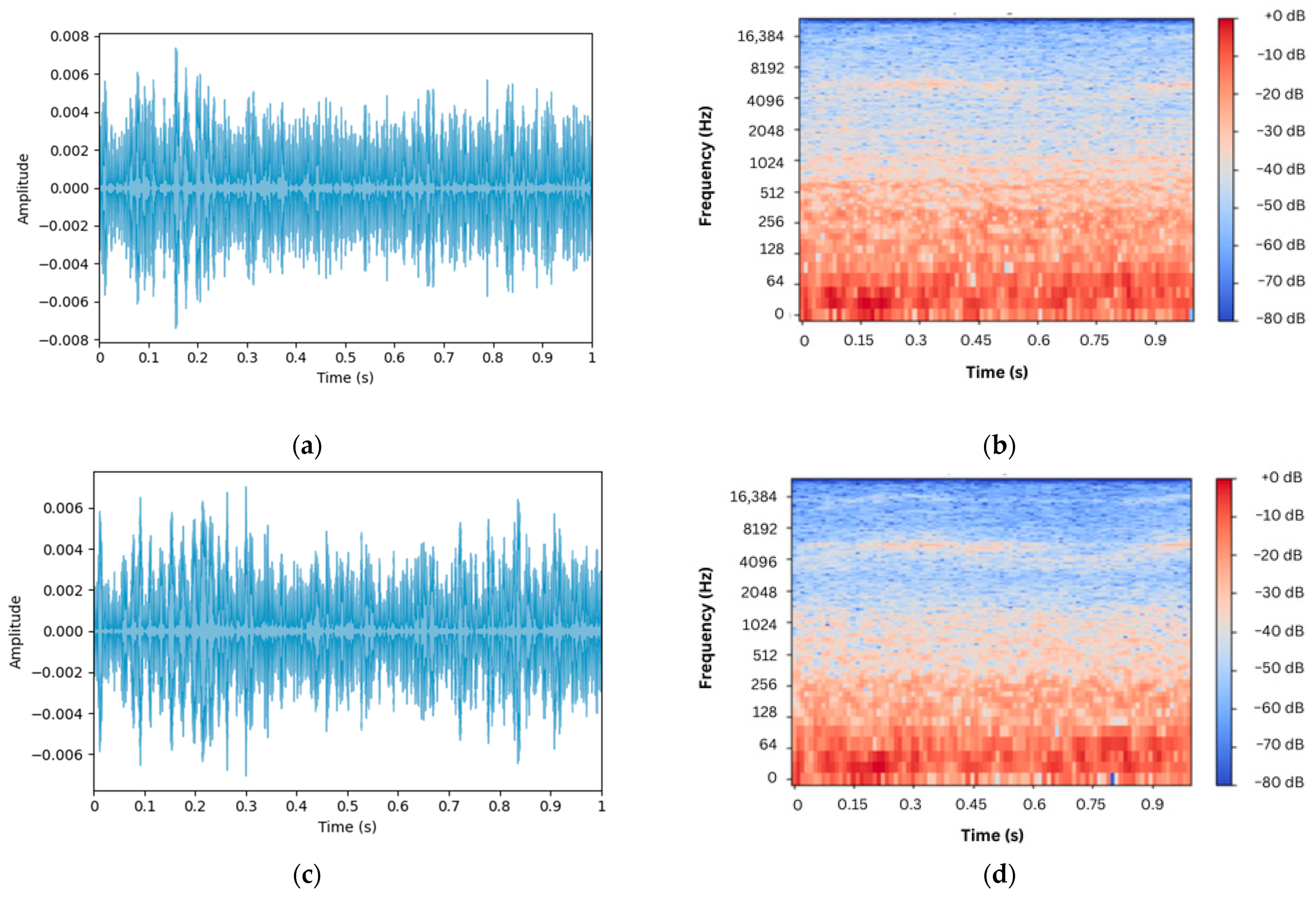
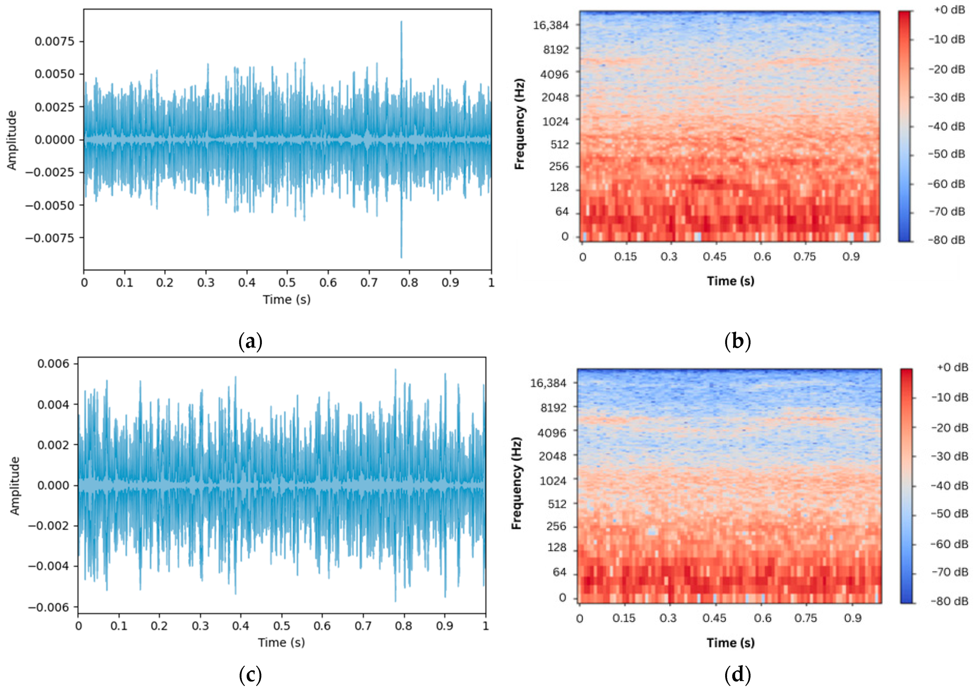
The recorded sounds, visualized as waveforms and spectrograms in Figure 6, reveal subtle differences between recordings near and farther away from the hive in the presence of intrusion. Specifically, Figure 6a,b depict the waveform and spectrogram of the acoustic sound collected near the hive entrance, respectively, whilst Figure 6c,d depict those recorded farther from it. Acoustic recordings during normal scenarios, i.e., without the presence of intrusion, are shown in Figure 7; Figure 7a,b depict the waveform and spectrogram of the acoustic sound collected near the hive entrance, respectively, whilst Figure 7c,d depict those recorded farther from it. Clearly, it is almost impossible to differentiate between normal and alarm sounds merely by auditory or visual inspection alone, underscoring the need for a more effective way of differentiation between the two scenarios.

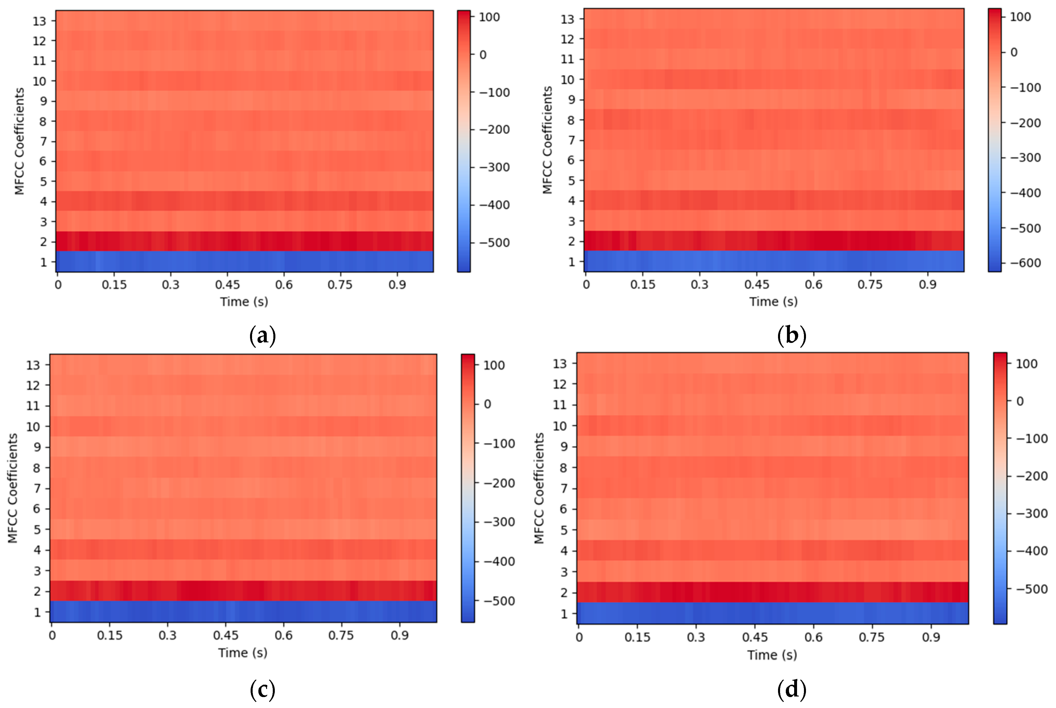
Following preprocessing, MFCC was extracted as the primary feature for classification. This extraction reduced each 1 s audio segment from 48,000 original data points to 1222 MFCC features, enabling more efficient processing without compromising essential sound information. Figure 8 illustrates these MFCC features, with Figure 8a,b showing the spectrogram of sounds recorded near and farther away from the entrance, respectively, during intrusion, and with Figure 8c,d showing the spectrogram of sounds recorded near and farther away from the entrance, respectively, in the absence of intrusion.

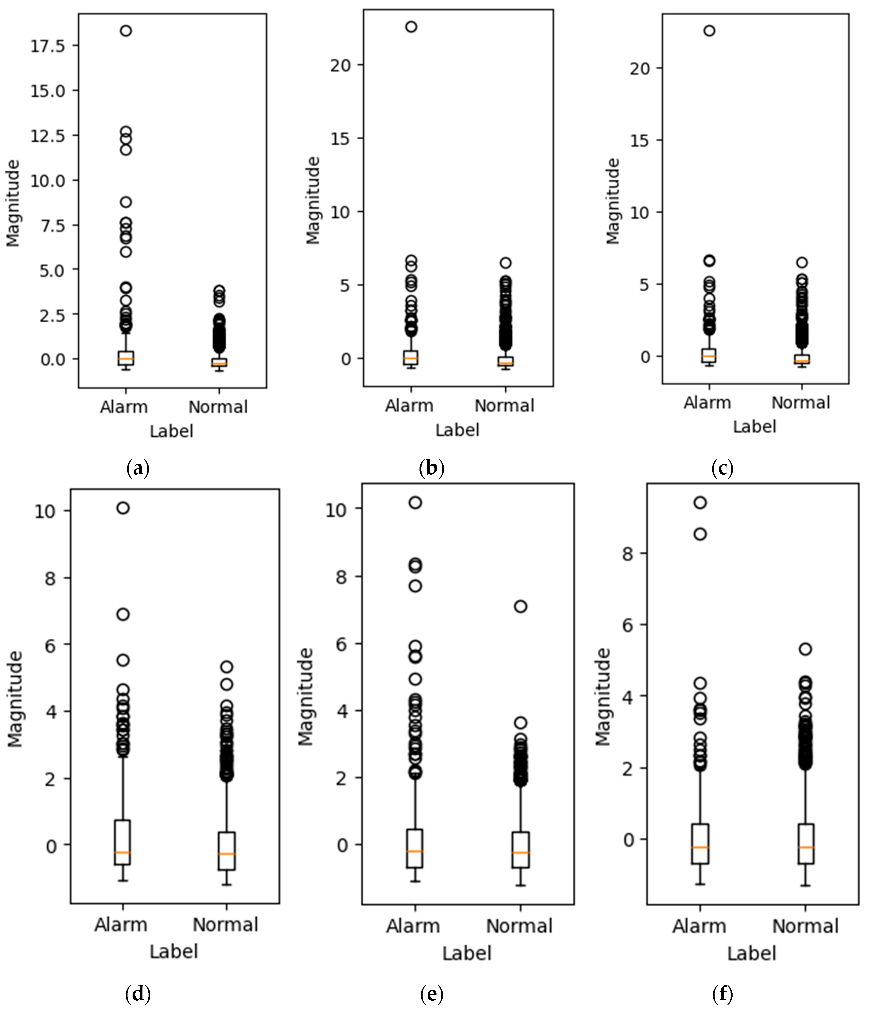
Box plots were generated for the average magnitude of each frequency bin for alarm and normal sounds after applying STFT. A total of 6 out of 1025 bins are shown in Figure 9. Both normal and alarm sound frequency bins contain outliers, which is primarily due to background noises such as other animals’ sounds and vehicle noise.

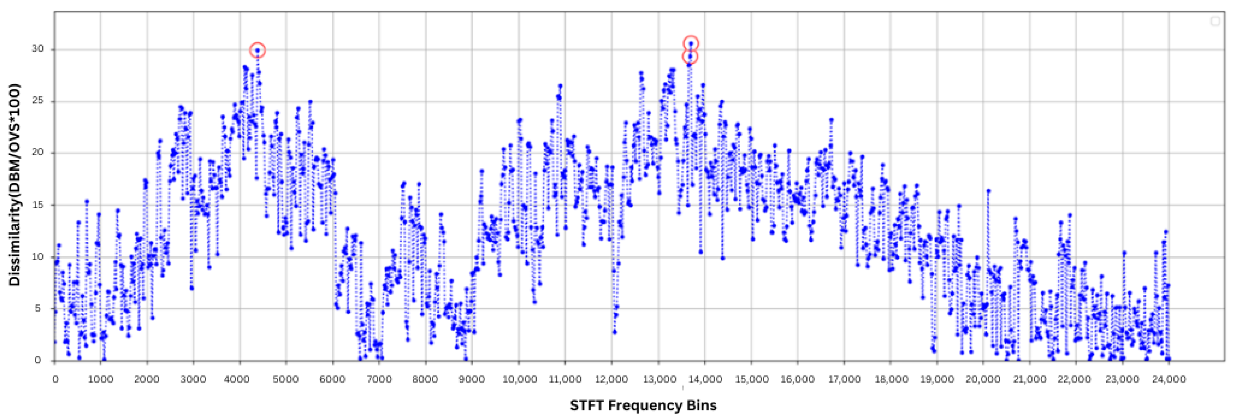
To further investigate the difference between alarm and normal acoustic data, DBM and OVS were calculated for each frequency bin. The dissimilarity (P) for each frequency bin was computed using Equation 1 and is presented in Figure 10. The results indicate that the magnitudes at frequency bins 4382.8125 Hz, 13,687.5 Hz, and 13,710.9375 Hz have significant differences between alarm and normal sounds, with p values of 29.95%, 29.37%, and 30.63%, respectively. These points are highlighted in the figure with red circles, demonstrating notable differences between normal and alarm sounds, even though both were recorded in the same environment.

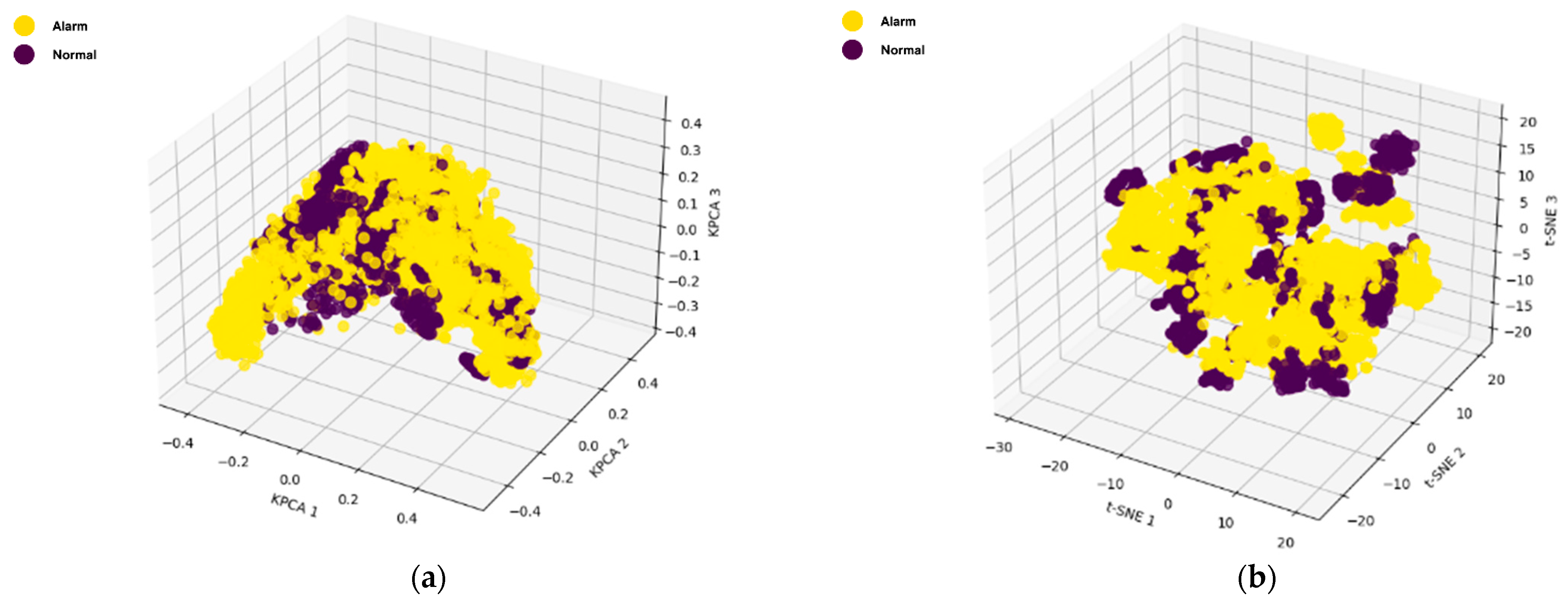
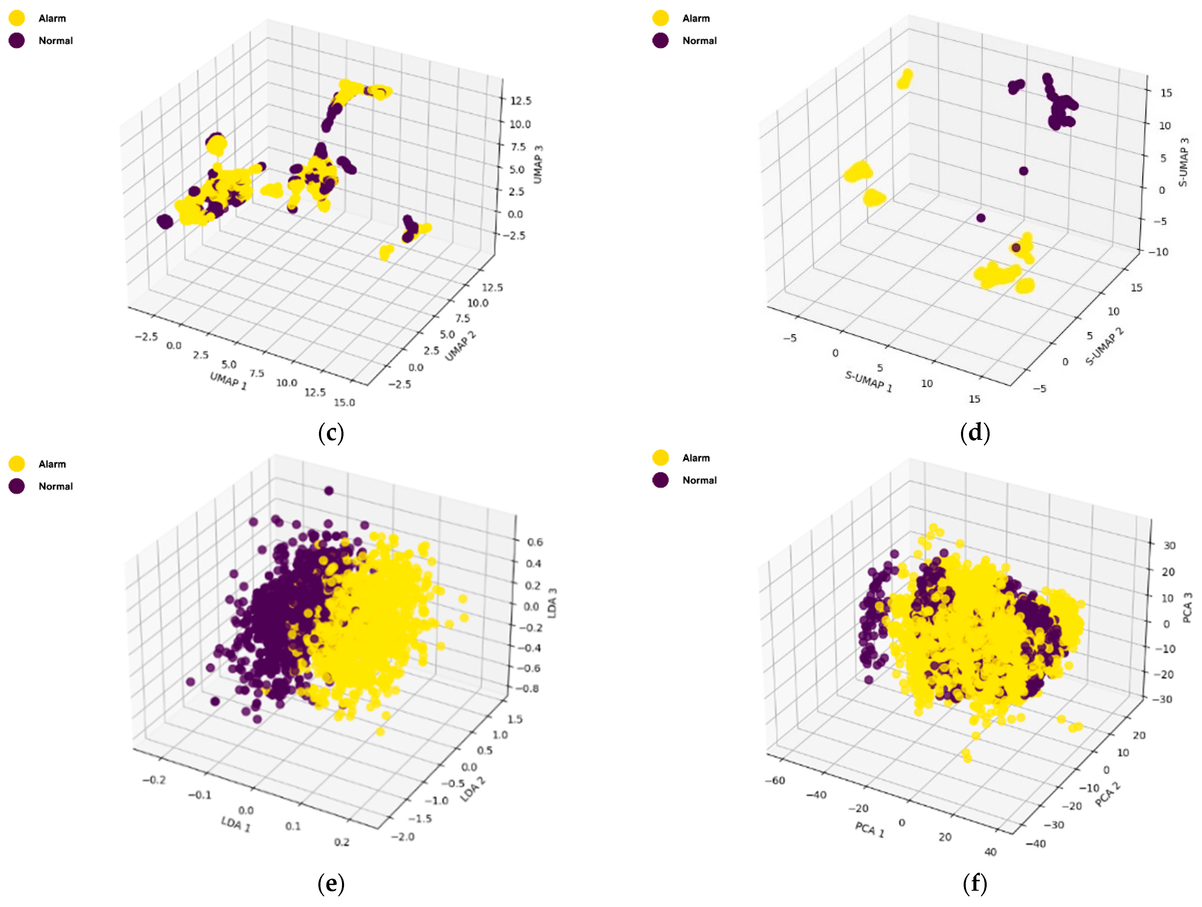
3.2. Dimensionality Reduction

To further streamline the feature set, six dimensionality reduction techniques, namely KPCA, t-SNE, UMAP, S-UMAP, LDA, and PCA, were applied, projecting the data into 3D space, as shown in Figure 11. In these visualizations, the “Alarm” class is represented by yellow points and the “Normal” class by purple points.

Among these techniques, LDA produced the most distinct clustering, effectively separating the two classes. This strong separation is likely due to LDA’s use of class label information, which optimizes for between-class variance, thereby enhancing the separation between “Alarm” and “Normal” sounds. Although S-UMAP creates more than two manifolds, it shows significant separation between two classes. LDA’s and S-UMAP’s superior performance in separating the “Alarm” and “Normal” classes likely stem from its inherent use of class label information to maximize separability between predefined classes. Unlike unsupervised methods like KPCA, t-SNE, UMAP, and PCA, which do not leverage class labels, LDA is a supervised technique that explicitly seeks to maximize the variance between classes while minimizing the variance within each class. This targeted approach enables LDA to create projections that are directly optimized for classification, making it highly effective for tasks with distinct, predefined categories.

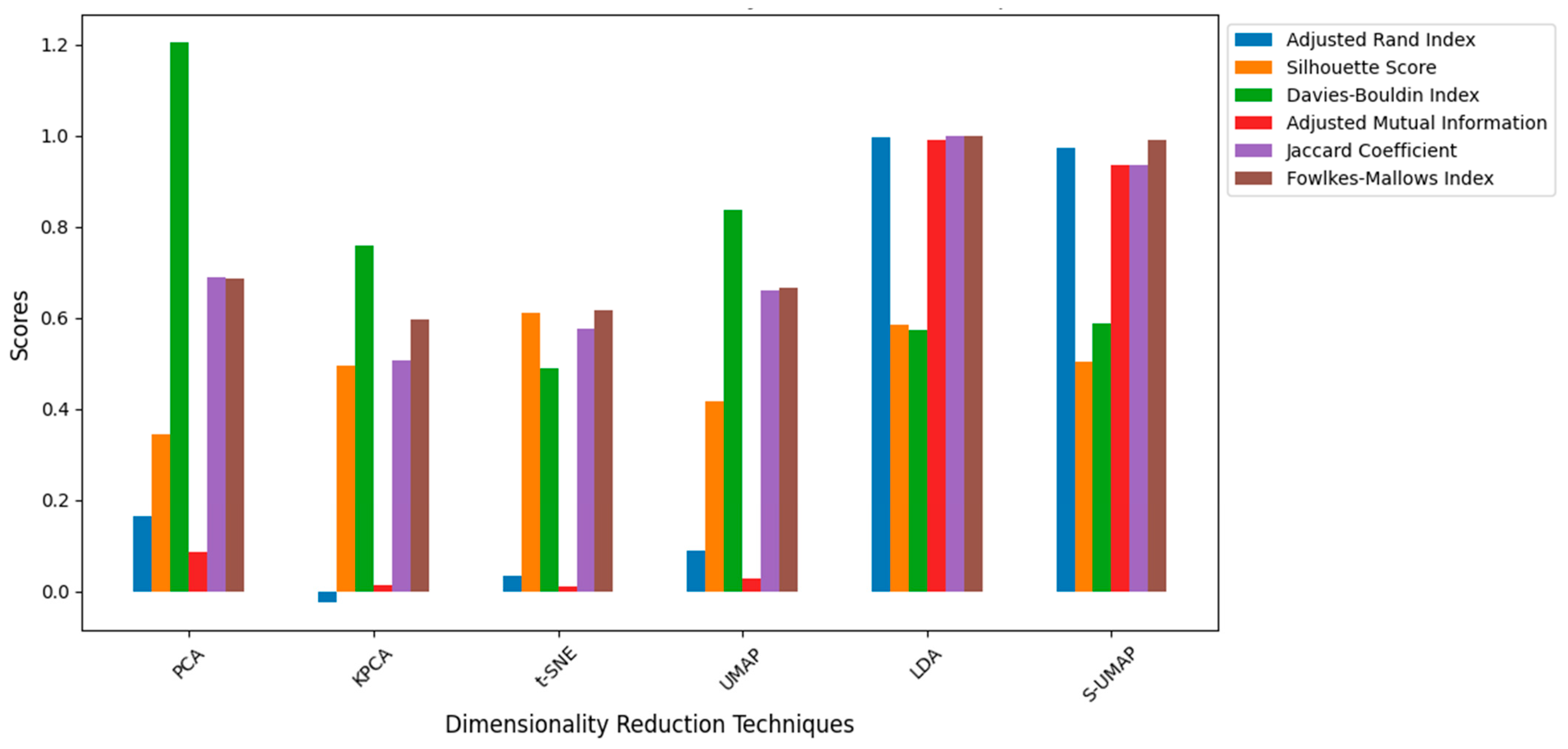
Clustering performance metrics were used to evaluate the effectiveness of dimensionality reduction techniques:

• Adjusted Rand Index (ARI): This metric ranges from −1 to 1, where a value of 1 indicates perfect clustering, meaning the predicted clusters match the true labels exactly.
• Silhouette Score: This score ranges from −1 to 1. A score close to 1 indicates well-separated clusters with clear boundaries, while scores near 0 suggest overlapping clusters. Negative values indicate incorrect clustering.
• Davies–Bouldin Index: This index measures cluster compactness and separation. Lower values indicate better clustering, with 0 being the ideal score, representing a perfect cluster separation and minimal overlap.
• Adjusted Mutual Information (AMI): This metric measures the information shared between true labels and predicted clusters, normalized to range between 0 and 1. A value of 1 indicates perfect clustering, accounting for chance alignment.
• Jaccard Coefficient: This coefficient ranges from 0 to 1, where a value of 1 indicates perfect overlap between the ground truth and predicted clusters.
• Fowlkes–Mallows Index (FMI): This index ranges from 0 to 1, where a value of 1 indicates perfect clustering with no misclassifications.

Figure 12 shows the performance of each dimensionality reduction technique based on the above-mentioned metrics. Consistent with the visual inspection results, LDA and S-UMAP demonstrated a generally better overall performance, achieving higher values for ARI, Silhouette Score, AMI, Jaccard Coefficient, and FMI, whilst also maintaining a lower Davies–Bouldin Index, which indicate better clustering. Notably, the clustering performance of the LDA was slightly better than the S-UMAP, making LDA the optimal one for this study. In contrast, PCA, KPCA, t-SNE, and UMAP exhibited moderate performance, with varying values across different metrics. Although KPCA, t-SNE, and UMAP are nonlinear dimensionality reduction techniques (NLDRTs), their impact was not significantly superior to the linear methods. This underscores the benefit of incorporating class information in dimensionality reduction, as seen with LDA and S-UMAP.

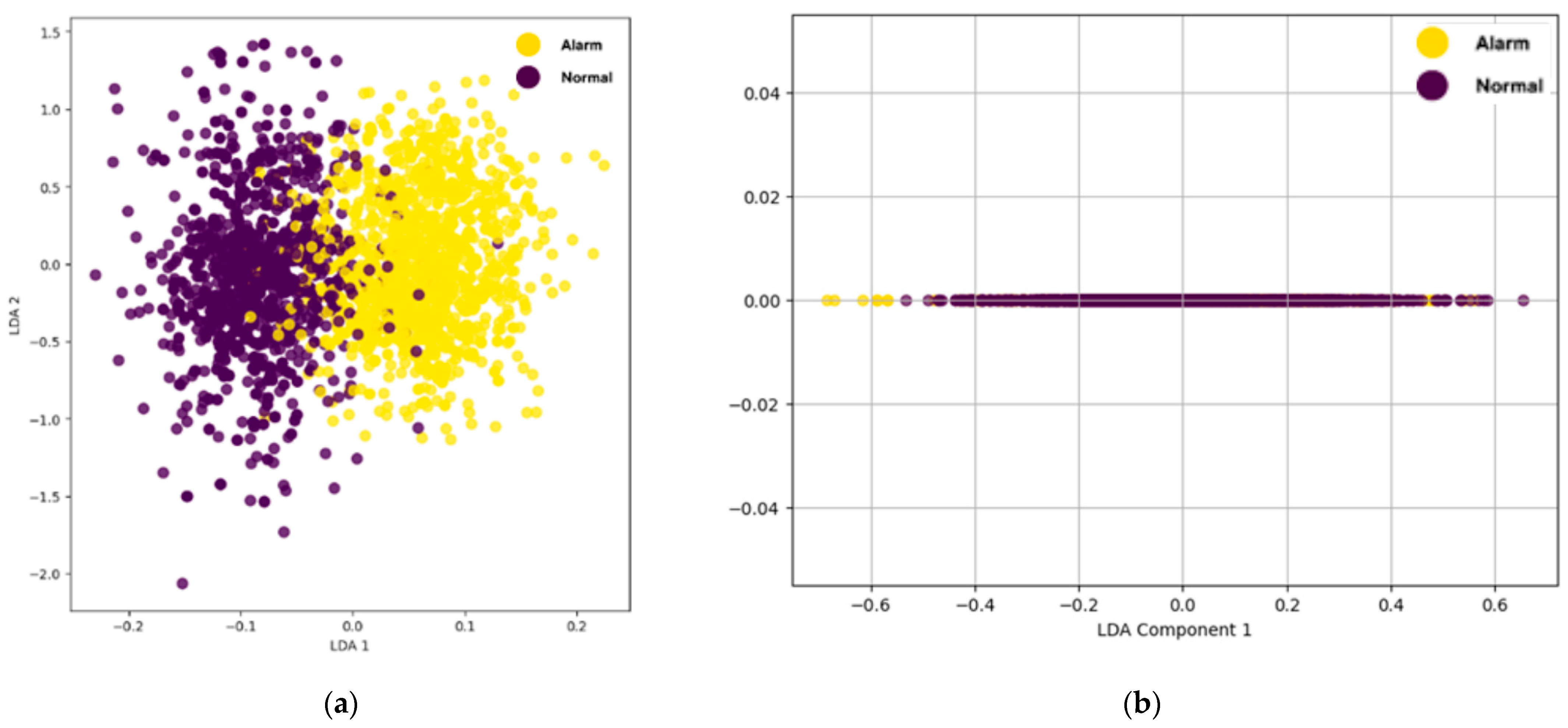
Additionally, the impact of further dimensionality reduction using LDA was explored by projecting features into two and one dimensions, as shown in Figure 13a,b, respectively. Figure 13a illustrates that feature reduction using LDA effectively enhances the separation between the “Alarm” and “Normal” classes in a 2D projection, while the 1D projection in Figure 13b demonstrates a significantly poorer performance with a substantial overlap between the classes. Despite the improved separation in 2D, some overlaps still remain, indicating that the distinction between classes is not entirely clear. This suggests that careful tuning of the number of retained features is essential to achieve an optimal classification accuracy; selecting an appropriate number of dimensions can enhance class separability, reduce misclassification rates, and improve the overall performance of the classification model.

3.3. Classification Performance

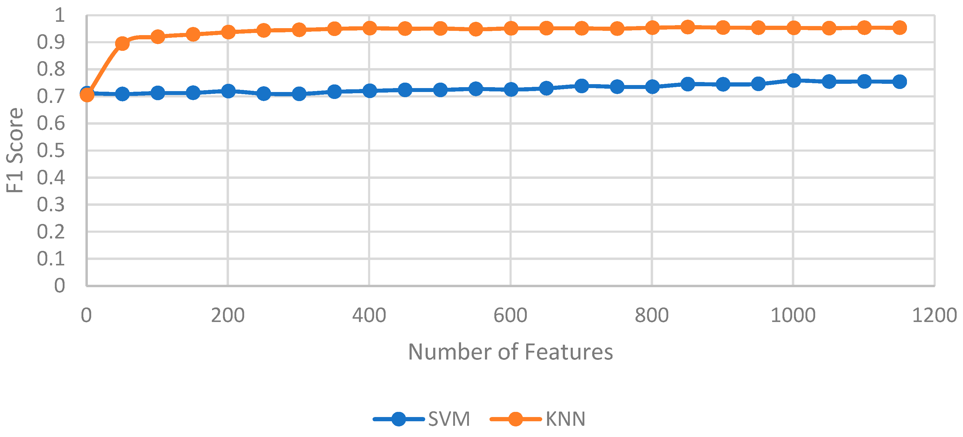
With the reduced feature sets, two classification models, KNN and SVM, were trained and evaluated to determine their optimal configurations. The optimal feature counts were determined experimentally, with KNN achieving its highest accuracy with 851 reduced features and with SVM performing best with 1001 reduced features, as shown in Figure 14. Additionally, the optimal number of neighbors k for KNN was identified as 1 through Grid Search, which consistently yielded a high accuracy across all cross-validation folds. This low k value suggests that the nearest neighbor of each data point effectively represents its class in this dataset, enhancing the KNN model’s classification performance.

Using k = 1 in KNN is advantageous in cases where the data have high class separability, meaning that instances from different classes are clearly distinct in the feature space. In such cases, each data point is likely to be closest to others of the same class, enabling accurate classification based on a single nearest neighbor. This also allows KNN to establish highly detailed decision boundaries, capturing subtle variations in acoustic patterns that may be meaningful in distinguishing between alarm and normal sounds. However, only considering the only nearest neighbor comes with certain trade-offs: the model is more sensitive to noise, as any outlier or mislabeled instance can directly affect classification. Additionally, it can increase the risk of overfitting, especially with training data containing inconsistencies. In contrast, higher k values generally improve robustness by averaging over a broader neighborhood and, hence, reducing the influence of anomalies. Nevertheless, the high-class separability on this dataset made k = 1 a suitable choice, allowing the model to accurately classify alarm sounds.

The confusion matrices and performance metrics for both models are shown in Figure 15 and

Table 4. Performance metrics of the SVM and KNN models.

Metrics	SVM	KNN (K = 1)
Number of Features	1001	851
Precision	0.7459	0.95265
Recall	0.7712	0.95862
F1 Score	0.7583	0.95563
Overall Cross-Validation Accuracy	75.42% ± 0.81%	95.54% ± 0.67%
Prediction Time (seconds)	0.037865	0.030907

, respectively. The metrics include traditional metrics such as Precision, Recall, and F1 Score, alongside the prediction time per instance, measured in a Google Colab environment (Processor: Intel(R) Xeon(R) CPU @ 2.20 GHz, RAM: 12.67 GB, Disk: 107.72 GB). As shown in Table 4, the KNN model consistently outperformed the SVM model across all evaluation metrics. KNN achieved a Precision of 0.95265, Recall of 0.95862, and F1 Score of 0.95563, which are significantly higher than the SVM metric scores of 0.7459, 0.7712, and 0.7583, respectively. Moreover, KNN attained an Overall Cross-Validation Accuracy of 95.54% (±0.67%), far surpassing SVM’s accuracy of 75.42% (±0.81%). The lower standard deviation in KNN’s cross-validation accuracy (0.67% versus SVM’s 0.81%) suggests a more stable performance across folds, indicating that KNN provides not only a higher accuracy but also more consistent results across different data splits. KNN also demonstrated faster prediction times, requiring only 0.0309 s per instance compared to 0.0379 s for SVM.

The superior performance of KNN over SVM in this study can likely be attributed to the nature of the feature space and underlying data characteristics. KNN’s instance-based learning approach is highly effective in cases where class boundaries are well-defined and data points from the same class are closely clustered in the feature space. This appears to be true for the MFCC features extracted from bee sounds, which naturally form distinct clusters, allowing KNN to form fine-grained decision boundaries. By setting k = 1, KNN capitalizes on the nearest-neighbor relationship, thus providing a highly localized classification decision that leverages the inherent separability of the data.

In contrast, SVM relies on finding an optimal hyperplane to separate classes, which may not perform as well if the data are not linearly separable or if there are subtle variations within classes that the hyperplane fails to capture. Although the kernel trick helps SVM capture non-linear boundaries, it may be less suited to datasets where local clusters, rather than global margins, define class distinctions. Additionally, SVM tends to be more sensitive to feature scaling and hyperparameter settings, which may affect its consistency in this classification context.

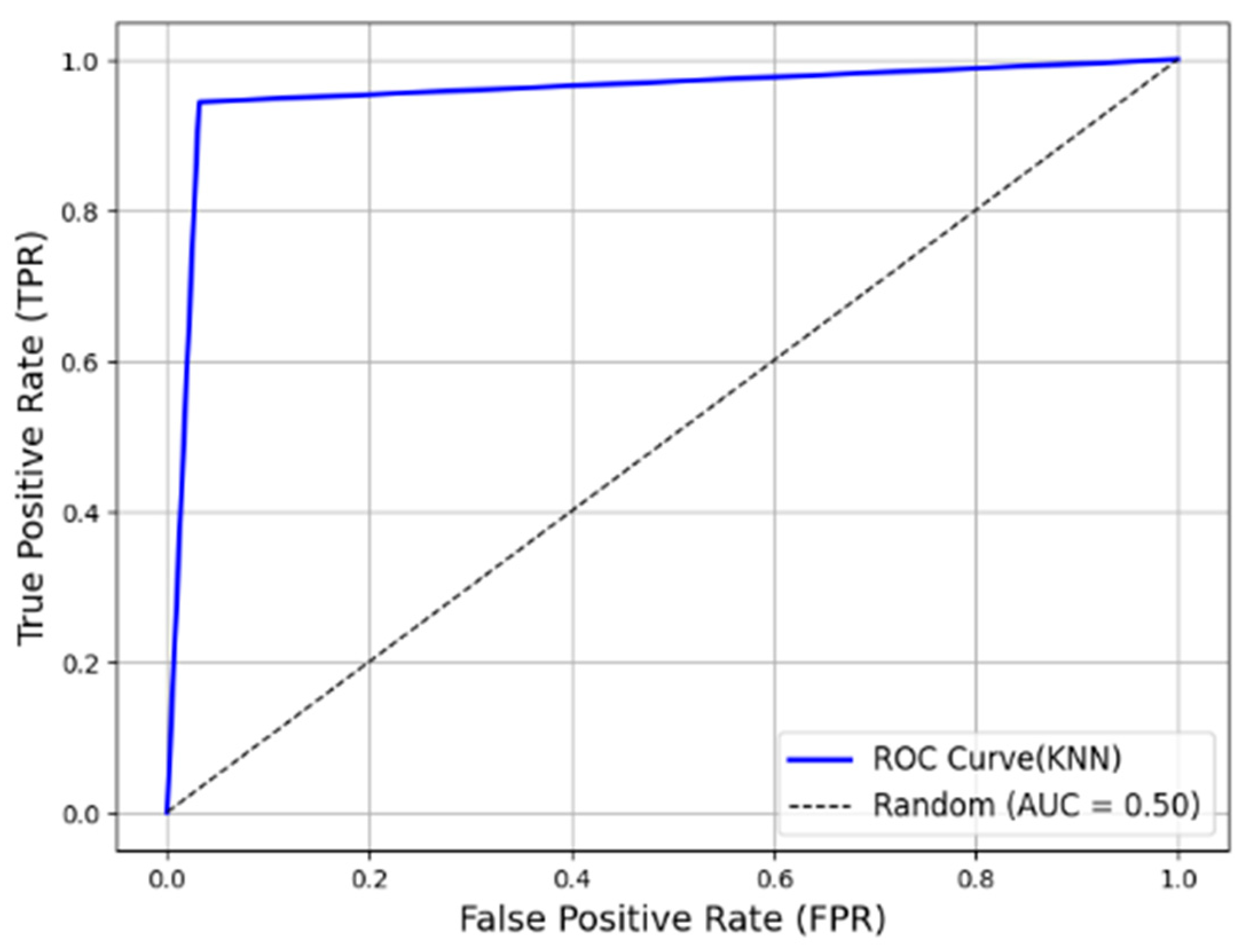
The Receiver Operating Characteristic (ROC) curve for the KNN model across five folds is shown in Figure 16. Since k = 1 in KNN, there are only three threshold values. The curve closely resembles that of a perfect model. Additionally, the average Area Under the Curve (AUC) score across the five folds is 0.9561, further validating the effectiveness of KNN as a single-number representation of model quality.

Although studies on alarm sounds or vibrations in bees are limited, most existing research focuses on honey bees rather than stingless bees. Additionally, the primary objective of many of these studies has been to confirm that bees emit distinct sounds during intrusions, rather than to computationally classify or analyze these signals. However, the computational identification of alarm signals is a crucial advancement for precision apiculture, as it enables automated hive monitoring and early threat detection [9,34].

In honey bees (Apini tribe), the hissing sound typically exceeds 3 kHz [35], and Papachristoforou et al. [9] reported that honey bees can produce sounds covering a wide frequency spectrum, with a dominant frequency of around 6 kHz in response to artificial hornet attacks. This may explain the significant dissimilarity observed in the frequency bin, albeit at a different frequency of 4382.8125 Hz in Figure 10, suggesting that stingless bees (Heterotrigona itama) may produce distinct alarm signals with characteristic frequency patterns.

To further investigate the results, Shapley Additive exPlanations (SHAP) [36] values were computed for the KNN classifier to analyze the contribution of MFCCs in decision-making. The impact of MFCCs on classification performance is illustrated in Figure 17a,b, where lower-order MFCCs exhibit a higher influence on the model’s decision-making process. Lower MFCC coefficients primarily represent the vocal tract shape or smooth spectral shape, whereas higher MFCC coefficients correspond to excitation information and periodicity in the waveform [37,38]. The significantly higher SHAP values associated with lower-order MFCC coefficients indicate that the overall spectral shape plays a more crucial role than pitch and periodicity in distinguishing alarm sounds from normal sounds. This suggests that stingless bee alarm signals exhibit a consistent spectral shape, ensuring that these signals are easily recognizable and trigger appropriate defensive or escape responses within the colony.

Overall, the superior performances of KNN in terms of both accuracy and computational efficiency makes it the preferred model for identifying the alarm sounds of H. itama bees. However, further analysis is needed to investigate the robustness of these models under varying noise levels and potential class imbalances, providing additional insights into their suitability for broader, real-world applications.

4. Conclusions

The objective of this study was to analyze and classify the alarm sounds produced by H. itama during intrusions using shallow learning algorithms. A custom data collection system was developed using a Jetson Nano, microphones, and camera to capture and label bee sounds with minimal disturbance to the bees. Subsequently, Mel-frequency cepstral coefficients (MFCCs) were extracted from the audio data as features, with multiple dimensionality reduction techniques evaluated to determine the best reduction techniques. Linear Discriminant Analysis (LDA) was demonstrated as the best in providing class separability.

For classification, K-Nearest Neighbors (KNNs) and Support Vector Machine (SVM) models were trained and tested. The results indicated that KNN significantly outperformed SVM with a Precision, Recall, and F1 Score of 0.9527, 0.9586, and 0.9556, respectively, and an Accuracy of 95.54% (±0.67%). This is compared to the lower accuracy of 75.42% (±0.81%) for SVM. Additionally, the Receiver Operating Characteristic (ROC) curve further validated the robustness of KNN, with an AUC of 0.9561, highlighting its high classification reliability.

These findings establish that H. itama emits distinct acoustic signals during intrusions, which can be effectively used for hive security and early threat detection. By utilizing sound-based monitoring, this approach offers a computationally efficient and cost-effective alternative to vision-based solutions, reducing both hardware costs and power consumption. Given the availability of commercial bee monitoring systems, integrating this intrusion detection feature would require only minimal additional hardware, such as two microphones, while leveraging existing processing units or mobile devices. The shallow machine learning algorithm used in this study ensures that computational requirements remain minimal, making real-time implementation feasible on edge devices. With a low implementation cost, this approach provides a scalable and affordable solution for beekeepers seeking to enhance hive security through bioacoustic monitoring.

Future research should explore the robustness of this method under different environmental conditions, varying noise levels, and potential class imbalances. Additionally, extending the study to other stingless bee species could further validate the generalizability of this technique in real-world beekeeping applications. Since the study utilized a simulated intrusion, further investigations should examine whether H. itama encodes threat-specific information in its alarm signals when responding to different types of natural enemies. Understanding these distinctions could enhance the application of bioacoustic monitoring for hive security and improve automated threat detection systems.