Evaluating Remote Sensing Resolutions and Machine Learning Methods for Biomass Yield Prediction in Northern Great Plains Pastures

Abstract

Predicting forage biomass yield is critical in managing livestock since it impacts livestock stocking rates, hay procurement, and livestock marketing strategies. Only a few biomass yield prediction studies on pasture and rangeland exist despite the need. Therefore, this study focused on developing a biomass yield prediction methodology through remote sensing satellite imagery (multispectral bands) and climate data, employing open-source software technologies. Biomass ground truth data were obtained from local pastures, where Kentucky bluegrass is the predominant species among other forages. Remote sensing data included spatial bands (6), vegetation indices (30), and climate data (16). The top-ranked features (52 tested) from recursive feature elimination (RFE) were short-wave infrared 2, normalized difference moisture index, and average turf soil temperature in the machine learning (ML) model developed. The random forest (RF) model produced the highest accuracy ($R^2=0.83$) among others tested for biomass yield prediction. Applications of the developed methodology revealed that (i) the methodology applies to other unseen pasters ($R^2=0.79$), (ii) finer satellite spatial resolution (e.g., CubeSat; 3 m) better-predicted pasture biomass, and (iii) the methodology successfully developed for a combination of Kentucky bluegrass and other forages, extended to high-value alfalfa hay crop with excellent yield prediction accuracy ($R^2=0.95$). The developed methodology of RFE for feature selection and RF for biomass yield modeling is recommended for biomass and hay forage yield prediction.

1. Introduction

In the Northern Great Plains region of United States, rangeland forage productivity is greatly influenced by climatic factors such as precipitation and temperature [1]. North Dakota, situated northeast of the Great Plains, has a continental climate and experiences naturally occurring drought and significantly varying temperatures. Local ranchers and livestock producers face the challenge of ensuring forage availability under these typical varying climatic conditions. Therefore, timely forage biomass production estimation during the growing season in rangeland and pastures can aid in making efficient management decisions for livestock production.

Traditional methods of biomass yield monitoring and prediction for pasture and rangeland involves hand clipping and drying the biomass for mass measurements from the randomly placed quadrats across a large landscape [2,3]. This conventional method is time-consuming and therefore not performed frequently during the growing season. Moreover, continuous monitoring of the biomass production data aids ranchers in making and adapting real-time management decisions.

Remote sensing (RS), an alternative methodology, has proved effective in nondestructive, extensive, and repetitive coverage of land areas, making it the perfect technology for continuous monitoring of growth in rangeland and pastures. The RS data include imagery from satellite and UAV platforms. Visible, thermal, multispectral, and hyperspectral bands captured by the RS sensors have been used to validate the clipped biomass [4,5]. Over the last few years, high spatial and temporal resolution satellites, such as Landsat, Sentinel, and CubeSat satellite platforms, having 30, 10, and 3 m spatial resolutions, respectively, are freely available and increasingly accessible, which makes periodic yield monitoring achievable. Some of the free imagery sources for these satellites are Google Earth Engine, PlanetScope Inc. and the U.S. Geological Survey.

Satellites record multispectral bands, including visible, near-infrared (NIR), and short-wave infrared imagery (SWIR), which were used to estimate vegetation indices (VIs). These indices provide indications of vegetation characteristics such as greenness, photosynthetic activity, and moisture content [6,7,8]. Some of the most commonly used VIs are normalized difference vegetation index (NDVI), enhanced vegetation index (EVI), and atmospherically resistant vegetation index (ARVI), among many others [9]. The effect of climate variables on crop growth has been extensively documented, and long-term studies have shown a strong relationship between climate and plant growth [10]. In addition to climate, soil plays an imperative role in affecting the growth of plants; warm soil temperature induces better water and nutrient uptake and contributes to the overall plant growth [11].

Biomass yield is a combination of spatial and temporal changes, and the variability can be captured by satellite, climate, and soil data [12]. The data (satellite, climate, and soil) are strongly linked and present themselves as nonlinear and complex interactions in predicting crop yield. Complex interactions among the dependent and independent variables, in recent times, have been widely analyzed using machine learning (ML) and are therefore ideal for agricultural applications. The ML models have been suitable for applications such as crop yield predictions, nutrient management, species identification, weed detection, and many others [13,14,15].

In general, better performances by ML models than by traditional linear regression models were reported [16,17,18]. The essential factors of yield estimation using ML were (i) the identification of the most important independent variables using feature selection methods, (ii) development of suitable prediction models, and (iii) calibration and validation of the developed ML models.

Selection of important climate, soil, and VI (satellite) features for crop yield prediction has been performed using feature selection methods such as Boruta, recursive feature elimination, information gain, sequential feed-forward selection, Relief, and many others [19,20,21]. Among the developed ML models, random forest (RF) has been widely used in predicting crop and forage biomass yield predictions [22,23,24]. Many studies involving soil, climate, and VIs have reported good performance using support vector regression (SVR) in predicting yield [25,26]. For instance, for predicting winter wheat yield in China using climate, soil, and remote sensing data, SVR emerged as one of the best ML models [27]. Several studies have also tested the performance of k-nearest neighbor (kNN) methods for yield prediction [28].

With this background and research opportunity, a study was designed to develop yield prediction models for pasture biomass using climate and satellite-based multispectral images. The specific objectives for pasture biomass prediction included (i) determining the potential use of climate variables and multispectral images (non-destructive method) for biomass prediction and (ii) identifying and recommending an overall methodology of the best features selected and ML model based on the prediction accuracy. The validity of the developed methodology (selected features and trained ML models) will be further assessed through three key applications: (i) evaluating the predictive performance of the methodology on unseen data from different pastures; (ii) analyzing the impact of spatial resolution on predictive accuracy for pasture biomass; and (iii) testing the predictive performance of the selected methodology on other forage crops.

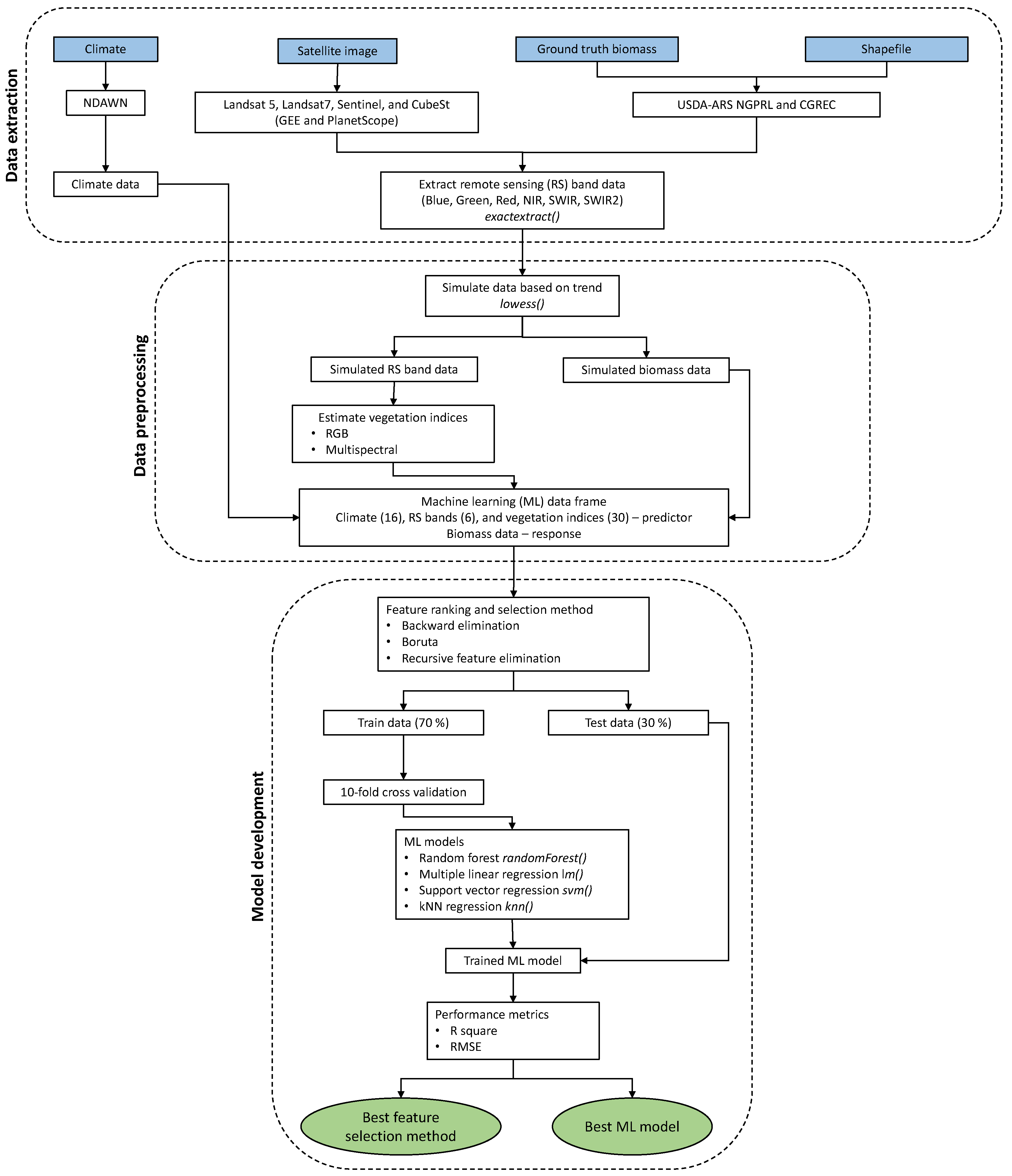
2. Materials and Methods

2.1. Study Site Description

The study sites were located at the Northern Great Plains Research Laboratory (NGPRL; USDA-ARS), Mandan, North Dakota 46°46’12” N 100°55’59” W; Figure 1). North Dakota receives peak precipitation occurring during June–July (3–4 inch) with an annual average precipitation of 17.9 inches. The average high temperature was recorded in July (28 °C), and the average low temperature recorded was in January (–2 °C).

The NGPRL site included three pastures, out of which two were native vegetation pastures and one was seeded forage pasture [29]. The former two are historical pastures, (i) a heavily grazed pasture (HGP; 2.8 ha) and (ii) a moderately grazed pasture (MGP; 15.4 ha); were initiated in 1916; and are maintained without using fire, fertilizer, or herbicides. The crested wheatgrass pasture (CWP; 2.6 ha), once native, was seeded in 1932. Vegetation in MGP was dominated by Kentucky bluegrass (Poa pratensis L.), an invasive cool-season grass. Blue grama [Bouteloua gracilis (Willd. ex Kunth) Lag. ex Griffiths], a warm-season native grass, dominated the HGP pasture until 2010 and was too dominated by the Kentucky bluegrass. A mix of crested wheatgrass [Agropyron desertorum (Fisch. ex Link) J.A. Schultes] and Kentucky bluegrass can be found in CWP. The fields were within 1 km of each other. Among the pastures, the data from the MGP pasture were used to train the prediction models, while CWP and HGP data were used for model testing.

2.2. Data Acquisition

The methodology followed in this study including data extraction, data preprocessing, and model development is depicted in Figure 2. Various details of the processes involved are described subsequently.

2.2.1. Ground Truth Biomass Data

The forage data at NGPRL were collected as above-ground live biomass every 2–3 weeks from mid-April to late September or mid-October (growing season) in the CWP, HGP, and MGP pastures for the years 2004–2006 and 2017–2018. The biomass was clipped from four representative samples using 0.25 m2 quadrats. The collected biomass was dried at 60–80 °C and weighed for moisture content measurements.

2.2.2. Climate and Soil Data

The pastures’ local weather data were obtained from the North Dakota Agricultural Weather Network (NDAWN) from the station located at NGPRL, Mandan, ND. Data at this station were available from 1999 to the present. Since the pastures were not far from each other, the same weather data were used for all pastures. Monthly data were obtained for nine climate and soil variables: average air temperature, bare soil temperature, turf soil temperature, wind speed, dew point, and chill and total values of solar radiation, potential evapotranspiration (PET), and rainfall (

Table 1. Climate and remote sensing data considered for this study.

Remote Sensing Data (Satellite Platforms)						Climate Data (NDAWN)
No.	Parameter	Abbreviation	Availability			No.	Parameter	Abbreviation
			Landsat	Sentinel	CubeSat
	Surface Reflectance Bands:						Weather Variables:
1	Blue (0.45–0.52 $\mathsf{\mu }$m)	B	✓	✓	✓	37	Air temperature (minimum, °C)	Min_T
2	Green (0.52–0.60 $\mathsf{\mu }$m)	G	✓	✓	✓	38	Air temperature (average, °C)	Avg_T
3	Red (0.63–0.69 $\mathsf{\mu }$m)	R	✓	✓	✓	39	Air temperature (maximum, °C)	Max_T
4	Near-infrared (0.77–0.90 $\mathsf{\mu }$m)	NIR	✓	✓	✓	40	Air temperature (diurnal range, °C)	Di_TR
5	Short-wave infrared 1 (1.57–1.75 $\mathsf{\mu }$m)	SWIR1	✓	✓	–	41	Bare soil temperature (°C)	AvgB_Soil
6	Short-wave infrared 2 (2.09–2.35 $\mathsf{\mu }$m)	SWIR2	✓	✓	–	42	Turf soil temperature (°C)	AvgT_Soil
	Color Vegetation Indices:					43	Wind speed (average, km/h)	Avg_WindS
7	Red chromatic coordinate	RCC	✓	✓	✓	44	Wind speed (maximum, km/h)	Max_WS
8	Green chromatic coordinate	GCC	✓	✓	✓	45	Wind direction (average,°)	Avg_WD
9	Blue chromatic coordinate	BCC	✓	✓	✓	46	Total solar radiation (Ly)	Tot_Sol_R
10	Excess green	ExG	✓	✓	✓	47	Potential evapotranspiration (Penman, mm)	Pen_PT
11	Normalized excess green	ExG2	✓	✓	✓	48	Potential evapotranspiration (Jensen-Haise, mm)	JH_PET
12	Excess red	ExR	✓	✓	✓	49	Total rainfall (mm)	Rainfall
13	Excess green minus excess red	ExGR	✓	✓	✓	50	Dew point (average, °C)	Dew_P
14	Green-red vegetation index (VI)	GRVI	✓	✓	✓	51	Wind chill (minimum, °C)	Min_Wind_Chill
15	Green-blue VI	GBVI	✓	✓	✓	52	Wind chill (average, °C)	Wind_Chill
16	Blue red VI	BRVI	✓	✓	✓
17	Green-red ratio	$G/R$	✓	✓	✓
18	Green-red difference	$G-R$	✓	✓	✓
19	Blue-green difference	$B-G$	✓	✓	✓
20	Visible-band difference VI	VDVI	✓	✓	✓
21	Visible atmospherically resistant index	VARI	✓	✓	✓
22	Modified green-red VI	MGRVI	✓	✓	✓
23	Colour index of vegetation	CIVE	✓	✓	✓
24	Woebbecke index	WI	✓	✓	✓
25	Coloration index	CI	✓	✓	✓
	Multispectral Vegetation Indices:
26	Normalized difference VI	NDVI	✓	✓	✓
27	Green normalized VI	GNDVI	✓	✓	✓
28	Soil-adjusted VI	SAVI	✓	✓	✓
29	Modified soil-adjusted VI	MSAVI	✓	✓	✓
30	Enhanced VI	EVI	✓	✓	✓
31	Normalized difference moisture index	NDMI	✓	✓	–
32	Green atmospherically resistance VI	GARI	✓	✓	✓
33	Simple ratio index	SR	✓	✓	✓
34	Atmospherically resistant VI	ARVI	✓	✓	✓
35	Green chlorophyll index	GCI	✓	✓	✓
36	Structure intensive pigment index	(SIPI)	✓	✓	✓

Note: VI—vegetation index; spatial resolution: Landsat—30 m, Sentinel—30 m, CubeSat—3 m, and NDAWN—North Dakota Agricultural Weather Network.

). This monthly weather data were exported as a CSV file, a format suitable for reading and processing.

2.2.3. Satellite Image Data

The remote sensing data for 2004–2006 (NGPRL study site) were retrieved from the Landsat archive of the Google Earth Engine (GEE) using JavaScript. Satellite images were obtained from GEE for the growing season spanning April to October. Monthly images were processed in GEE by calculating the average for each month to reduce temporal variability and enhance consistency. These averaged images were then downloaded for further analysis. The Landsat images are available once every two weeks from 1972 to the present day and provide satellite images of the earth’s surface using seven spectral bands at 30 m spatial resolution. Satellite data for the pastures were obtained by creating a rectangular extent (as JSON) including all three pasture areas (CWP, HGP, and MGP) for the three years from Landsat 5 (Thematic Mapper, TM) and Landsat 7 (Enhanced thematic mapper, ETM) [30]. The TM images were mostly used for data collection, while ETM images were only used in the case where TM images were missing or no cloud-free TM images were available. The Landsat images from the ’Tier 1’ category of the GEE datasets were considered for their higher data quality and level of processing. Atmospheric factors such as aerosols and thin clouds are accounted for by using the atmospherically corrected datasets using surface reflectance from the TM and ETM sensors. Additionally, these Tier 1 and surface reflectance data were further screened for clouds, snow, and shadows using the CFMask() function [31].

Remotely sensed data for the years 2017–2018 for the NGPRL study sites were collected from Sentinel-2. The Sentinel-2 images have been available since 2015 once every ten days with a spatial resolution ranging from 10 to 30 m. The multi-spectral instrument (MSI) sensor in the Sentinel-2 platforms generates an image with 13 spectral bands ranging from visible to short-wave infrared. PlanetScope imagery from Planet Labs Inc. was used to download raw Sentinel-2 images. The satellite image tile covering the study site pastures was selected with cloud cover condition less than 20%. The raw Sentinel images obtained were preprocessed for atmospheric correction. The semi-automatic classification plugin available in QGIS (version 3.16) software was used for performing atmospheric correction for the Sentinel images using the provided metadata [32].

2.3. Data Processing

The approach to obtaining various VIs, representing the forage growth specific to the study pastures, is to overlay the pasture’s shapefiles on the satellite images and extract relevant spatial and band information for data processing. The satellite image data processing was performed in open-source QGIS and R (version 4.1.1) software. Shapefiles were generated using the New Shapefile Layer (polygon) option in QGIS. A shapefile vector layer with three polygons was created for the NGPRL pastures to perform image processing analysis. The downloaded Landsat satellite images were a single raster layer consisting of multiple bands (eight) as stacks. In contrast, the images from Sentinel-2 were a single raster layer consisting of multiple bands (11 in total). These multiple bands from Sentinel-2 were stacked using the R function stack() to form a multi-band raster layer.

The five major bands commonly used in estimating plant characteristics are blue (B), green (G), red (R), near-infrared (NIR), short-wave infrared (SWIR), and short-wave infrared 2 (SWIR2) and were stripped from the stacked raster layers for estimating VIs (Table 1). A stripped band (raster layer) was overlaid onto the pasture shapefile (vector layer) for extracting the band value for the pastures’ shapefiles. The extraction was performed through zonal statistics using the exact_extract() R function. The zonal statistics results presented the mean value of the pixels (band data) available in the polygon created for each pasture. This satellite image processing was repeated for all the satellite images downloaded. Therefore, a user-coded function in R was created to automate the process of stacking, stripping, and applying zonal statistics for the bands.

2.4. Estimation of Vegetation Indices

The VIs derived by combining spectral bands can be attributed to various plant characteristics, including growth, water content, pigments, and protein content, among others [33]. The VIs were estimated from the selected spectral bands ( B, G, R, NIR, SWIR, and SWIR2) from the Landsat and Sentinel-2 images. A list of RGB-based and multispectral-based vegetation indices commonly used in various applications is presented in Table 2. The estimation of VIs had to be repeated multiple times over different dates for the satellite images. To automate this process, a user-coded R function was created to execute the estimation of VI (Table 1).

Table 2. List of RGB-based and multispectral-based vegetation indices.

Vegetation Index	Equation	Reference
Red chromatic coordinate (RCC)	${\displaystyle \frac{R}{R+G+B}}$	[34]
Green chromatic coordinate (GCC)	${\displaystyle \frac{G}{R+G+B}}$	[34]
Blue chromatic coordinate (BCC)	${\displaystyle \frac{B}{R+G+B}}$	[34]
Excess green (ExG )	$2G-B-R$	[34]
Normalized excess green (ExG2)	${\displaystyle \frac{B}{R+G+B}}$	[34]
Excess red (ExR)	${\displaystyle \frac{1.4R-G}{R+G+B}}$	[35]
Excess green minus excess red (ExGR)	$\mathrm{ExG}2-\mathrm{ExR}$	[36]
Green-red vegetation index (GRVI)	${\displaystyle \frac{G-R}{G+R}}$	[37]
Green-blue vegetation index (GBVI)	${\displaystyle \frac{G-B}{G+B}}$
Blue red vegetation index (BRVI)	${\displaystyle \frac{B-R}{B+R}}$
Greed-red ration (G/R)	${\displaystyle \frac{G}{R}}$	[38]
Green-red difference (G-R)	$G-R$
Blue-green difference (B-G)	$B-G$
Visible-band difference vegetation index (VDVI)	${\displaystyle \frac{2G-R-B}{2G+R+B}}$	[39]
Visible atmospherically resistant index (VARI)	${\displaystyle \frac{G-R}{G+R-B}}$	[40]
Modified green-red vegetation index (MGRVI)	${\displaystyle \frac{G^2-R^2}{G^2+R^2}}$	[41]
Colour index of vegetation (CIVE)	$0.441R-0.881G+0.385B+18.787$	[42]
Woebbecke index (WI)	${\displaystyle \frac{G-B}{R-G}}$	[34]
Coloration index (CI)	${\displaystyle \frac{R-B}{R}}$
Normalized difference vegetation index (NDVI)	${\displaystyle \frac{\mathrm{NIR}-R}{\mathrm{NIR}+R}}$	[43]
Green normalized vegetation index (GNDVI)	${\displaystyle \frac{\mathrm{NIR}-G}{\mathrm{NIR}+G}}$	[44]
Soil-adjusted vegetation index (SAVI)	${\displaystyle \frac{1.5(\mathrm{NIR}-R)}{\mathrm{NIR}+G+0.5}}$	[45]
Modified soil-adjusted vegetation index (MSAVI)	${\displaystyle \frac{2\mathrm{NIR}+1-\sqrt{{(2\left(\mathrm{NIR}\right)+1)}^2-8(\mathrm{NIR}-R)}}{2}}$	[46]
Enhanced vegetation index (EVI)	$2.5\times {\displaystyle \frac{\mathrm{NIR}-R}{1+\mathrm{NIR}+6R-7.5B}}$	[47]
Normalized difference moisture index (NDMI)	${\displaystyle \frac{\mathrm{NIR}-\mathrm{SWIR}}{\mathrm{NIR}+\mathrm{SWIR}}}$	[48]
Green atmospherically resistant vegetation index (GARI)	${\displaystyle \frac{\mathrm{NIR}-(G-(B-R\left)\right)}{\mathrm{NIR}+(G-(B-R\left)\right)}}$	[44]
Simple ratio index (SR)	${\displaystyle \frac{\mathrm{NIR}}{R}}$	[49]
Atmospherically resistant vegetation index (ARVI)	${\displaystyle \frac{\mathrm{NIR}-2R-B}{\mathrm{NIR}+2R-B}}$	[50]
Green chlorophyll index (GCI)	${\displaystyle \frac{\mathrm{NIR}}{G-1}}$	[51]
Structure intensive pigment index (SIPI)	${\displaystyle \frac{\mathrm{NIR}-B}{\mathrm{NIR}+B}}$	[52]

Note: Red (R), blue (B), and green (G) bands recorded from the satellite platforms. The top and bottom groups, separated by the horizontal line, list the RGB-based and multispectral–based vegetation indices, respectively.

Table 2. List of RGB-based and multispectral-based vegetation indices.

Vegetation Index	Equation	Reference
Red chromatic coordinate (RCC)	${\displaystyle \frac{R}{R+G+B}}$	[34]
Green chromatic coordinate (GCC)	${\displaystyle \frac{G}{R+G+B}}$	[34]
Blue chromatic coordinate (BCC)	${\displaystyle \frac{B}{R+G+B}}$	[34]
Excess green (ExG )	$2G-B-R$	[34]
Normalized excess green (ExG2)	${\displaystyle \frac{B}{R+G+B}}$	[34]
Excess red (ExR)	${\displaystyle \frac{1.4R-G}{R+G+B}}$	[35]
Excess green minus excess red (ExGR)	$\mathrm{ExG}2-\mathrm{ExR}$	[36]
Green-red vegetation index (GRVI)	${\displaystyle \frac{G-R}{G+R}}$	[37]
Green-blue vegetation index (GBVI)	${\displaystyle \frac{G-B}{G+B}}$
Blue red vegetation index (BRVI)	${\displaystyle \frac{B-R}{B+R}}$
Greed-red ration (G/R)	${\displaystyle \frac{G}{R}}$	[38]
Green-red difference (G-R)	$G-R$
Blue-green difference (B-G)	$B-G$
Visible-band difference vegetation index (VDVI)	${\displaystyle \frac{2G-R-B}{2G+R+B}}$	[39]
Visible atmospherically resistant index (VARI)	${\displaystyle \frac{G-R}{G+R-B}}$	[40]
Modified green-red vegetation index (MGRVI)	${\displaystyle \frac{G^2-R^2}{G^2+R^2}}$	[41]
Colour index of vegetation (CIVE)	$0.441R-0.881G+0.385B+18.787$	[42]
Woebbecke index (WI)	${\displaystyle \frac{G-B}{R-G}}$	[34]
Coloration index (CI)	${\displaystyle \frac{R-B}{R}}$
Normalized difference vegetation index (NDVI)	${\displaystyle \frac{\mathrm{NIR}-R}{\mathrm{NIR}+R}}$	[43]
Green normalized vegetation index (GNDVI)	${\displaystyle \frac{\mathrm{NIR}-G}{\mathrm{NIR}+G}}$	[44]
Soil-adjusted vegetation index (SAVI)	${\displaystyle \frac{1.5(\mathrm{NIR}-R)}{\mathrm{NIR}+G+0.5}}$	[45]
Modified soil-adjusted vegetation index (MSAVI)	${\displaystyle \frac{2\mathrm{NIR}+1-\sqrt{{(2\left(\mathrm{NIR}\right)+1)}^2-8(\mathrm{NIR}-R)}}{2}}$	[46]
Enhanced vegetation index (EVI)	$2.5\times {\displaystyle \frac{\mathrm{NIR}-R}{1+\mathrm{NIR}+6R-7.5B}}$	[47]
Normalized difference moisture index (NDMI)	${\displaystyle \frac{\mathrm{NIR}-\mathrm{SWIR}}{\mathrm{NIR}+\mathrm{SWIR}}}$	[48]
Green atmospherically resistant vegetation index (GARI)	${\displaystyle \frac{\mathrm{NIR}-(G-(B-R\left)\right)}{\mathrm{NIR}+(G-(B-R\left)\right)}}$	[44]
Simple ratio index (SR)	${\displaystyle \frac{\mathrm{NIR}}{R}}$	[49]
Atmospherically resistant vegetation index (ARVI)	${\displaystyle \frac{\mathrm{NIR}-2R-B}{\mathrm{NIR}+2R-B}}$	[50]
Green chlorophyll index (GCI)	${\displaystyle \frac{\mathrm{NIR}}{G-1}}$	[51]
Structure intensive pigment index (SIPI)	${\displaystyle \frac{\mathrm{NIR}-B}{\mathrm{NIR}+B}}$	[52]

Note: Red (R), blue (B), and green (G) bands recorded from the satellite platforms. The top and bottom groups, separated by the horizontal line, list the RGB-based and multispectral–based vegetation indices, respectively.

2.4.1. Common RGB Bands

The RGB color system is the most used for digital image processing. As RGB bands correspond to the visible range of the electromagnetic spectrum, true-color composites can be generated using these spectral bands. In addition to viewing, the three bands can be mathematically combined (VIs) to extract further information. Most of the RGB-based VIs were developed to highlight the greenness and spectral variation within the vegetation. Among the RGB-based VIs, excess green index (ExG) produced using the R, G, and B bands were the most commonly used to estimate greenness [34]. Based on the derived spectral bands from the Landsat and Sentinel-2 platforms, 19 RGB-based vegetation indices were computed for biomass prediction in the pastures (Table 2).

2.4.2. Multispectral

The sensors in the Landsat and Sentinel-2 were equipped to capture information in the electromagnetic spectrum that are not visible to the human eye. These multispectral bands are NIR and SWIR bands. Multispectral VIs were calculated mathematically by combining multispectral bands and/or RGB bands. The normalized VI is the most widely used multispectral VI and is estimated using the NIR and R bands [43]. The NDVI values ranged between $-1$ and +1, where −1 and +1 represent poor and healthy vegetation, respectively. NDVI proved successful in estimating canopy cover and vigor; however, it was sensitive to the effects of soil, atmosphere, and cloud. Therefore, 10 multispectral VIs were utilized to validate the pasture biomass (Table 2).

2.5. Modeling Approaches

The ML modeling techniques were used to predict the pasture biomass through selected features. Different wrapper-based feature selection methods were employed to compare and choose the best features representing the pasture biomass. Using the best features, various ML models were considered to predict the biomass and were compared within the selected ML models and against the simple multiple linear regression (MLR) models. The feature selection and prediction models considered are presented in detail in the subsequent subsections.

2.6. Feature Selection

The features included in this study are the extracted satellite band values (6), estimated VIs (RGB: 19, multispectral: 10), and climate variables (16), totaling 51 variables (Table 1). Among these features, understandably, some were more relevant in predicting pasture biomass than others. Feeding all the variables into machine learning models (including the irrelevant features) would impact the accuracy and increase the computation load and time. To address this, a wrapper-based feature selection method was employed.

In the wrapper-based feature selection process, a subset of the most relevant features are selected from a dataset, and features are either removed or added based on training a model and the inference obtained. In this study, three wrapper feature selection algorithms—namely, Boruta, recursive feature elimination, and stepwise regression—were used to estimate the relevant features. Correlation and mutual information were used to validate the results of the selected feature selection algorithms.

2.6.1. Backward Elimination

Backward elimination is one of the three most popular simple filter-based feature selection methods; the other two are forward selection and stepwise regression. It is a wrapper-based feature selection algorithm that initially considers all the features to build MLR models. The R function step() was used to run the backward elimination algorithm [53]. The MLR model was used to estimate the features with less relevance based on the calculated Akaike information criterion (AIC). Like adjusted R-squared, the AIC also penalizes the model performance while using an increased number of unnecessary variables. In this process, some features considered significant at an early stage may be eliminated later. In general, backward elimination produced a better subset of features since it was evaluated for significance by comparing it with the other features [54]. Therefore, only backward elimination feature selection was considered for this study.

2.6.2. Boruta

Boruta is a wrapper-based method built using a random forest (RF) algorithm that determines variable importance measures by default [55,56]. The Boruta feature selection method was implemented by using the Boruta() R package [57]. In the Boruta algorithm, for each feature, a shadow feature was created, and the values were obtained by randomly shuffling the values of the original feature. This extended dataset was subjected to the RF to evaluate the important features. The number of RF iterations performed on the extended dataset containing the original and shadow features was 120. At every iteration, the maximum Z-score of the shadow features (maximal importance of the random features, MIRA) was calculated for comparison with the Z-score of the individual original feature. The algorithm hypothesizes that the importance of the original feature is equal to or higher than the estimated MIRA, and when the hypothesis holds true, the number of hits (N) is recorded from the total iteration. An original feature was considered significant if the value of the hits was at least $0.5N$.

2.6.3. Recursive Feature Elimination

Recursive feature elimination (RFE) is a wrapper-based algorithm built around the random forest (RF, Section 2.7.3) model to yield the optimum features [20,58]. In R, the RFE feature selection was performed using the rfe() function in the caret package [59]. The RFE method initially employed all the features and eliminated the feature with the least RMSE calculated from the out-of-bag (OOB) data. A new RF model was developed using the remaining features. The process was recursively applied by employing 10-fold cross-validation (repeated 5 times) to optimize the variable selection process and select the most important features. At every run of this recursive process, the RF model with the selected subset of features yielding the least RMSE was considered optimum. However, the rank of the features was updated when another model with a different subset of features yielded the minimum RMSE. The RFE estimated the best subset of features yielding a minimum RMSE value through this repeated process.

2.7. Linear and Machine Learning Prediction Models

The features were ranked based on the feature importance results from backward elimination, Boruta, and RFE. Then, the ranked features were fed to select the linear and ML models, MLR, RF, support vector regression (SVR), and k-nearest neighbor (kNN) (Figure 2). The number of feature data fed into the ML models increased successively by one feature; the ML models were analyzed using the highest-ranked feature, and the process was repeated by including the second-highest feature and so on.

2.7.1. Training, Validation, and Test Datasets

The original dataset containing selected features from the feature selection methods (predictors) and pasture biomass (response) was subjected to random splitting with replacement for obtaining training and test data. The R function sample() was used to perform the data splitting operation. The partition ratio considered for the training and test datasets was 70 and 30, respectively (Figure 2). The 10-fold cross-validation method was used to validate the performance of the developed ML model. The training and validation datasets were used to train the prediction models, while the test dataset was used to estimate the accuracy of the trained models. The models developed using the training dataset were run 10 times to measure the accuracy of the test dataset; the partition ratio yielding consistent accuracy was considered optimum.

2.7.2. Multiple Linear Regression

MLR statistical models are simpler compared to their ML counterparts but have the advantage of being easy to calculate and comprehend and can be considered as a “control” model to compare ML models. These models use two or more predictor variables to explain the outcome of one response variable by fitting a linear equation [60,61]. In R, the MLR was performed using the lm() function [62]. The model assumes a linear relationship between the predictor and response variables, and the predictor variables are not highly correlated. Each value of the predictor variables was associated with the response variable, and the model determined a regression coefficient that had the least overall model error.

2.7.3. Random Forest

The RF is an ensemble learning algorithm (ML) with a collection of several decision trees [63,64]. The function ranger() in R was used to perform RF analysis. In RF, random samples were drawn from the train data with replacement using the bootstrap aggregating (bagging) method to avoid overfitting [65]. The random samples selected from the training data are called in-bag data and constitute 64% of the training data, while the remaining 36% of the samples are called the OOB data. Decision trees in RF are built independently using in-bag data, and a random subset of features is selected at each node where the feature importance is assigned based on the prediction accuracy. The OOB data were used to validate the built decision trees and the resulting mean-square error determined the prediction accuracy and variable importance. The final predictions for regression-based RF were obtained by averaging the prediction results from all the trees (bagging).

2.7.4. Support Vector Regression

The SVR is a supervised ML algorithm developed to predict discrete values [66,67]. The SVR algorithm in R was performed using the function svm() from the library “e1071”. The principles of SVR are similar to those of the support vector machine and use kernel functions to project the data onto a hyperspace to represent complex nonlinear patterns [68]. Kernel functions of SVR include sigmoid, polynomial, nonlinear, and radial basis function (RBF); however, only RBF was used for this study for its proven performance [69]. The SVR provides flexibility by defining the amount of error acceptable to the model and determining the best-fit line within that allowed threshold value. The threshold value is the distance between the hyperplane (best-fit line) and the boundary called the maximum error $ϵ$ (epsilon). The value of epsilon can be tuned to obtain the desired SVR model accuracy.

2.7.5. k-Nearest Neighbors

The kNN is an instance-based learner where, for each test data instance, the model finds the k samples nearest to the training data based on the distance value and averages their responses [14,70]. The “caret” package in R with the method option selected as “kNN” was used to implement the algorithm. The k value is always an odd number and plays a significant role in determining the model’s accuracy. A small k value might lead to poor accuracy if noise is present in the data, while a large k value might ignore the noise in the data but would significantly increase the computation load. An optimum k value can be estimated based on the model’s accuracy obtained from a selected range of k values.

2.8. High-Performance Computing Resources Used

Selecting features and training ML models, especially with RFE, are computationally intensive, involving a large number of repetitive calculations. Such computational loads cannot be efficiently handled by local computers (ordinary laptops or desktops), specifically during the developmental stage where several iterations are involved. Therefore, we used the North Dakota State University’s Center for Computationally Assisted Science and Technology (CCAST) high-performance computer clusters. An example of performance comparison with a single run using OnDemand RStudio Server IDE (https://kb.ndsu.edu/it/page.php?id=130346, university registered login credentials required, accessed on 25 February 2025) is as follows: the runtime for the RFE feature selection method on CCAST (system time: 719 s; 1 node and 4 cores with a 16 GB RAM configuration at basic service level) is on an average 1.5 times faster (other calculations up to 2.5 times) than the local system (system time: 1127 s). The performance of the CCAST basic service level can be improved further by requesting more resources. It was observed that the use of systems like CCAST or similar is necessary while developing ML models involving several variables (multispectral image bands and climate data).

2.9. Model Performance Assessment

2.9.1. Hypertuning Parameters

The best performance of ML models is not guaranteed with the default hyperparameter settings; therefore, their hyperparameters need to be tuned to achieve the best predictions [71]. The ML models considered for this study were all subjected to hyperparameter tuning to determine the robust estimates. Tuning can be performed by manually selecting the parameters; however, automatic selection is recommended for estimating the optimum parameter. The RF models involved several hyperparameters such as the number of trees involved (num.trees), the number of variables randomly selected at each split (mtry), and the minimum observation at each node (min.node.size). The number of trees tested was 500, 1000, and 1500, while the mtry value was set to p/3 (default value for regression) where p is the total number of features, and min.node.size was set to 5 (default value for regression).

All these RF hyperparameters were used in the grid search operation. With SVR, the essential parameters were kernel, epsilon ($ϵ$), cost, and gamma. Kernels are crucial in SVR since they use the data for transitioning into higher-dimensional space. $ϵ$ determines the width of the tube around the hyperplane (decision boundary) developed using the RBF function. The cost function in SVR determines the softness of the margin, and the gamma determines the shape of the decision boundary; a high gamma value results in more curvature. The values considered for $ϵ$ were between 0 and 1, while the cost values ranged between $2^2$ and $2^9$, and the gamma values considered were 0.001, 0.1, 1, and 3. The kNN model used a range of k values between 5 and 9 with an increment of 1 for determining the optimum based on the accuracy.

2.9.2. Performance Metrics

The robustness of the models was determined using 10-fold cross-validation repeated ten times. The performance of the models was recorded using metrics such as coefficient of determination ($R^2$) and root-mean-square error (RMSE) for the predictions from ML regression models, which are represented in the following equations. A higher value of $R^2$ and a smaller value of RMSE represent a better prediction performance of the model tested.

$$R^2=1-{\displaystyle \frac{{\sum }_{i=1}^n{(y_i-{\widehat{y}}_i)}^2}{{\sum }_{i=1}^n{(y_i-{\overline{y}}_i)}^2}}$$

(1)

$$\mathrm{RMSE}=\sqrt{{\displaystyle \frac{1}{n}}\sum _{i=1}^n{(y_i-{\widehat{y}}_i)}^2}$$

(2)

where i = index of the observation, n = the number of observations, $y_i$ = the observed value, ${\widehat{y}}_i$ = the predicted value, and ${\overline{y}}_i$ = the mean of the observed values.

3. Results and Discussion

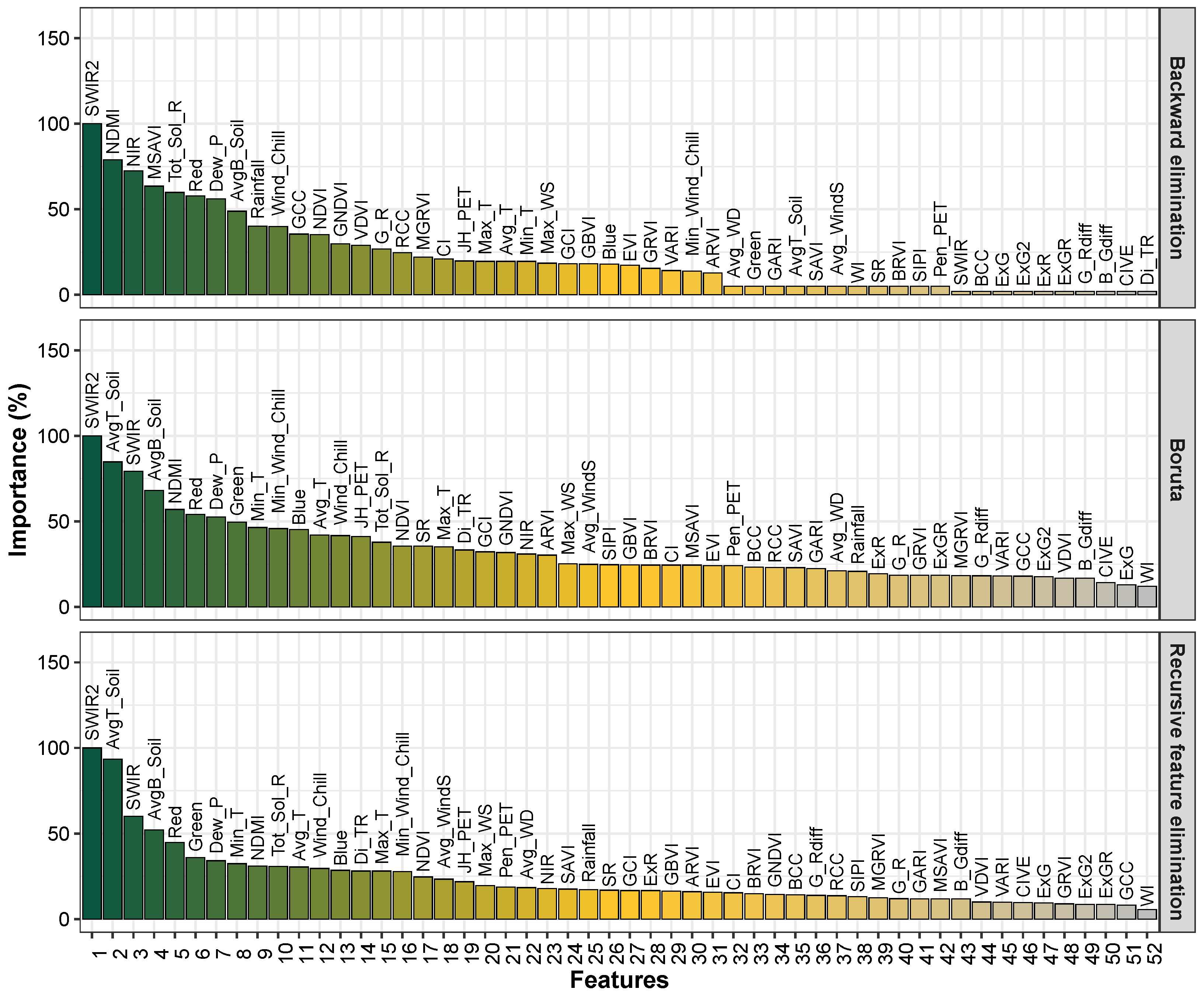
3.1. Feature Ranking Results

The 51 predictor features including climate, remote sensing bands, and VIs (Table 1) were ranked using the feature selection strategy described in Section 2.6. The ranking results from one pasture site (CWP) for the year 2006 are shown in Figure 3. Among the feature selection methods considered, the ranking differed, which reflected the unique techniques of the feature selection. However, similarities between the top-ranking features for the random forest-based feature selection algorithms, Boruta, and RFE methods were observed. The best feature for predicting biomass in the three methods was the SWIR2, a reflectance band captured by the satellite sensors. The band SWIR2 has been reported as one of the best wavelengths for estimating the fractional cover of vegetation and bare soil [72]. In addition to SWIR2, the red band ranked among the top six features in the feature selection methods and has been used in predicting yield in agricultural applications [73].

Several studies have reported the successful prediction of biomass yield using the NDMI, also known as the drought index [74,75]. The important climate variables are average wind speed (Avg_WindS) and average turf soil temperature (AvgT_Soil). Among the vegetation indices, the normalized difference moisture index (NDMI) ranks as one of the top 4 features in all the feature selection methods. The NDMI is generated using the RS bands NIR and SWIR; it can be observed that the band SWIR ranks as the second most important variable in the Boruta and RFE feature selection methods.

It is interesting to note that wind speed, which is not an obvious choice of variable for explaining biomass yield, is ranked higher than several obvious variables such as rainfall, ExG, and so on. However, wind speed is a crucial parameter impacting evapotranspiration and soil erosion, thereby affecting crop yield. Wind speed also increases crop water requirements by increasing potential evapotranspiration as the accumulated humid air near the leaves is removed [76]. Furthermore, the turf soil temperature for grasses is essential for the growth of crops since the warm temperature provides a favorable condition for water and nutrient uptake and has been used in various agricultural studies [77,78].

The vegetation indices VARI and MGRVI, which commonly use combined band values of green and red, are ranked the lowest in predicting biomass yield. The climate variable rainfall did not contribute to predicting biomass yield data; therefore, it is ranked as one of the least important features. Interestingly, the 6 RS bands obtained are among the top 15 features for at least 2 feature selection methods. Though feature ranking is available for all the features, the optimum number of features required can be determined by sequentially feeding the ML models and observing the prediction accuracy.

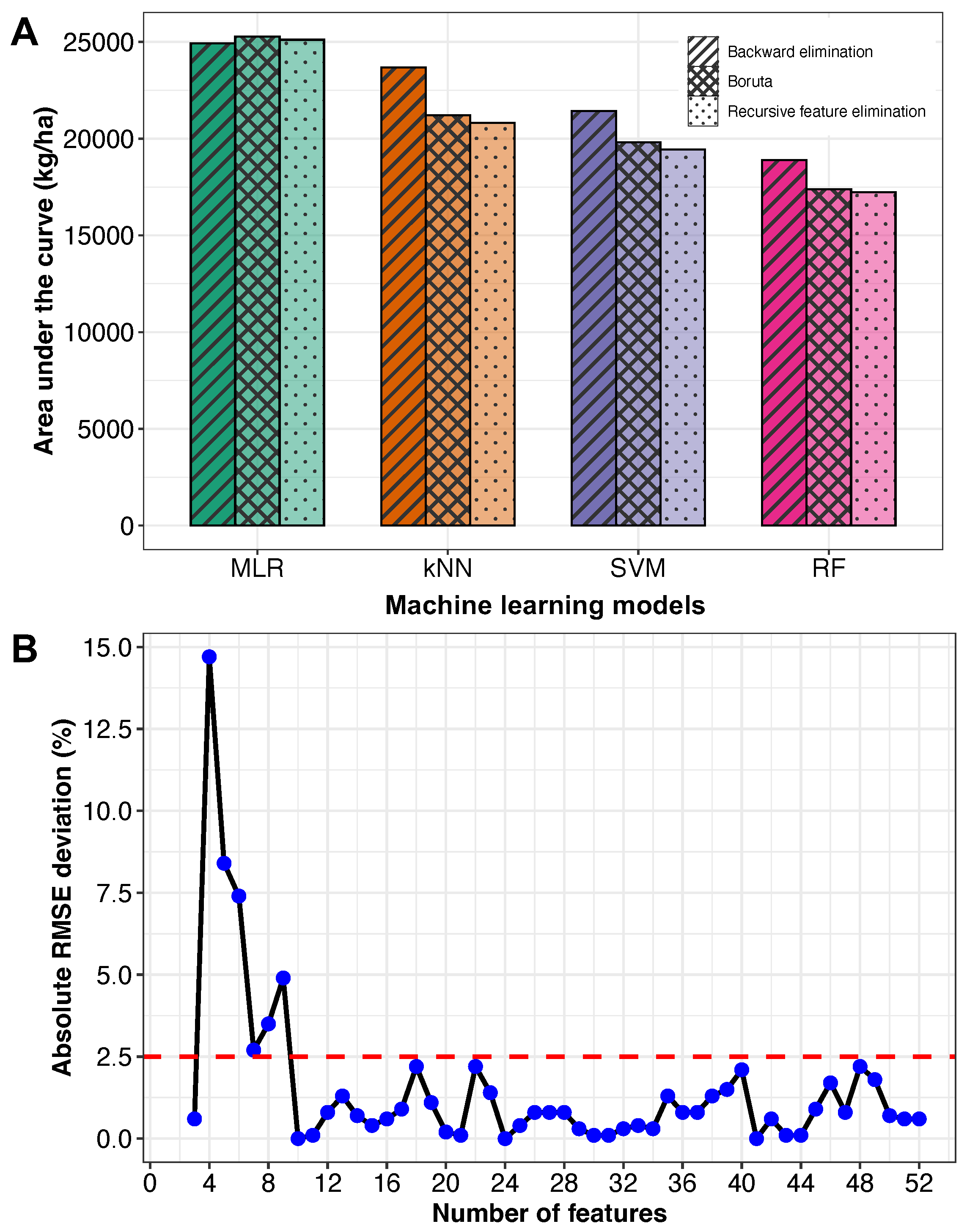
3.2. Feature Selection and Model Performance Comparison

The ranked features from the selected feature selection models for MGP pasture were fed sequentially, and the responses of the ML models were compared using RMSE metrics; a lower RMSE value implies higher model performance in predicting biomass. Based on the observed model responses, the best-performing feature selection method, the number of features, and ML models were determined.

3.2.1. Feature Selection Method Comparison

Overall, a decrease in RMSE was observed with an increase in the number of features across all the feature selection methods (Figure 4). However, a steep decrease in the RMSE trend was observed when there were fewer than 10 features. Among the feature selection methods, RFE recorded the lowest RMSE value across all the ML methods except MLR, indicating a better selection of important features.

For MLR, the backward elimination feature selection method performed the best because the wrapper-based backward elimination feature selection algorithm internally uses the MLR model to estimate the best features [79].

A comparable RMSE trend was observed for the feature selection methods Boruta and RFE because of their similar feature ranking as discussed in the previous section (Section 3.1). The average percentage decrease in RMSE value for RFE compared to MLR and Boruta was 11% and 2%, respectively (Figure 5).

3.2.2. Machine Learning Models Comparison—Ranking

Among the ML models, the RMSE was the lowest for RF followed by SVM, kNN, and MLR across all the feature selection methods (Figure 4). As expected, the MLR model was the least accurate in biomass prediction since it assumes a linear relationship between the predictor and response variables. Previous studies also report similar dominance of ML models in yield prediction over the linear regression models [16,17,18]. With the increase in the number of features, a steady decrease in RMSE was observed for the MLR model for all the feature selection methods. For the other ML models (kNN, RF, and SVM), the lowest RMSE was observed when there were fewer than 10 features, and the addition of more features increased the RMSE values, indicating reduced performance of the ML models. This trend was strongly observed with the kNN model. The average reductions in RMSE of the ML models kNN, SVM, and RF compared to MLR were 13, 19, and 29% (Figure 5A).

Overall, RFE performed well in the most influential predictors selected for estimating the biomass yield. The RFE methodology has been widely used for evaluating remote sensing variables and climate in estimating pasture and forage yield prediction [58,80]. Among the ML models, RF performed better in biomass prediction. Previous ML comparison studies show that RF has proven to be efficient in agricultural applications for predicting crop yield and above-ground biomass [63,64]. Using the selected RFE and RF methodology, the absolute RMSE deviation percentage was estimated for each additional feature (Figure 5B). The cut-off value for selecting the features was fixed at 2.5% of the absolute RMSE deviation.

The results revealed that for every additional feature after 10, the deviation of absolute RMSE value was less than 2.5%. Therefore, the top 10 ranked features from RFE recommended for training the RF model were SWIR2, AvgT_Soil, SWIR, AvgB_soil, Red, Green, Dew_P, Min_T, NDMI, and Tot_Sol_R (Table 1). Based on these results, for studies that used combined climate and remote sensing data to predict pasture and forage biomass, the methodology RFE for feature selection and RF for building an ML prediction model is recommended.

3.3. Application of the Developed Methodology and Model

The validity of the developed methodology (Section 3.2) for RFE (feature selection) and RF (prediction model) was further explored by using it for three different applications, as follows.

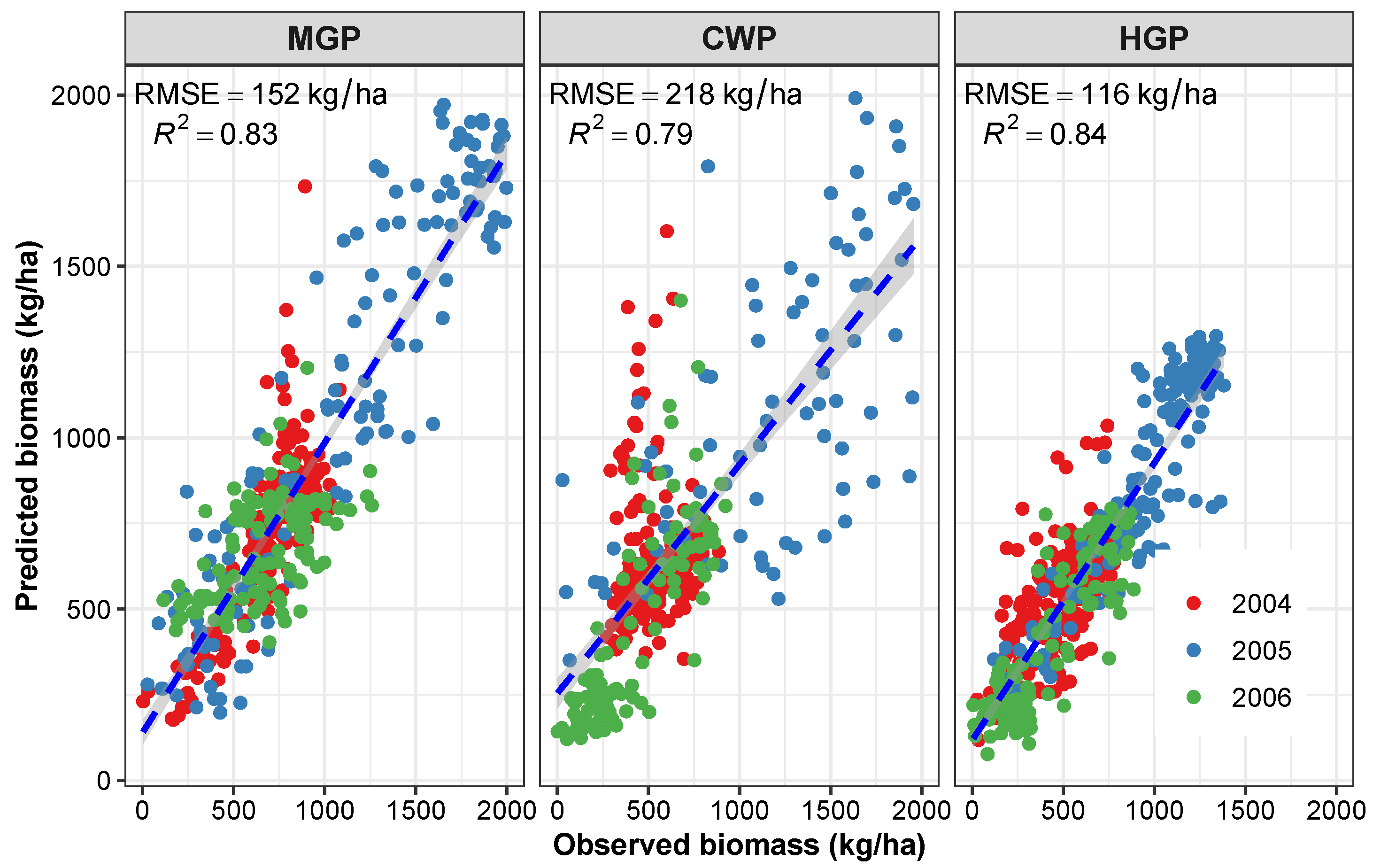
3.3.1. Application 1—Performance of the Developed Methodology in Other Pastures

The performance of the selected methodology based on the results from the MGP pasture was evaluated using the other two unseen pastures, CWP and HGP. Feature selection using RFE and RF model building were individually performed for the pastures CWP and HGP. Based on the feature selection results, the essential common features that emerged important in all the pastures are SWIR2, SWIR, Red, NDMI, AvgT_Soil, and AvgB_Soil (Table 1). The trend produced by testing (30% of the data) using the developed RF models in HGP ($R^2=0.84$) and MGP ($R^2=0.83$) was linear for 2004, 2005, and 2006, indicating a good correlation between the observed and predicted data (Figure 6).

However, a linear trend was more pronounced in HGP and MGP than CWP. For CWP, a good correlation was observed for biomass <1500 kg/ha ($R^2=0.79$); however, with increasing biomass, the trend showed a reduced correlation. It is vital to note that the ground truth data (observed) were no longer producing a clear growth curve for the CWP pasture.

In a different extended application, the prediction model assessment was explored by applying the trained RF model from the MGP pasture to the unseen biomass data from the CWP and HGP pastures. (Figure 7). The results showed that better predictions were obtained for the HGP pasture ($R^2=0.65$) followed by the CWP pasture ($R^2=0.37$). Comparable predictions were obtained for pastures MGP (developed ML model) and HGP since both the pastures were dominated by Kentucky bluegrass. Even though the CWP pasture contained Kentucky bluegrass, it was dominated by crested wheatgrass, which resulted in the lower performance of the trained ML model.

Overall, the selected methodology, which combines RFE and RF, was recommended for predicting biomass in other pastures due to its demonstrated ability to produce high accuracy. In a complementary application, the results of the model’s predictive performance revealed that the directly trained ML model (as opposed to the combined RFE and RF methodology), developed using the MGP pasture data, can effectively predict biomass for other pastures dominated by the same forage species (in this case, Kentucky bluegrass). This finding highlights the potential for applying trained ML models directly to pastures with similar soil and plant characteristics, offering a simpler and more practical approach. Developing such models for specific pastures or fields would enhance efficiency while maintaining accuracy.

3.3.2. Application 2—Effect of Remote Sensing Platforms Resolution in Forage Prediction

To evaluate the effect of satellite image resolution, the developed methodology (RFE and RF) was used to build models to validate MGP pasture biomass using bands and VI features sourced from three different satellite platforms with varying resolutions, such as Landsat, Sentinel, and CubeSat, along with climate features obtained from NDAWN for the years 2017 and 2018 (Figure 8). The top 10 features from the RFE for MGP with different satellites are presented in

Table 3. Feature ranking from recursive feature elimination for satellite platforms.

Rank	Landsat	Sentinel	CubeSat
1	AvgT_Soil	AvgT_Soil	AvgT_Soil
2	Green	Di_TR	NIR
3	G_Rdiff	SWIR2	GCI
4	SWIR2	Tot_Sol_R	MSAVI
5	SWIR	Avg_WindS	GNDVI
6	AvgB_Soil	AvgB_Soil	SAVI
7	Blue	SWIR	AvgB_Soil
8	SIPI	Avg_WD	Blue
9	BCC	NDMI	RCC
10	Di_TR	JH_PET	NDVI

Note: Please refer to Table 1 for more information on the features.

. It was observed that the band values of SWIR and SWIR2 were influential in predicting biomass in the pasture for Landsat and Sentinel platforms. However, in CubeSat, with the absence of SWIR or SWIR2 bands, the NIR band emerged as the best predictor band feature.

Studies have reported that CubeSat NIR with fine resolution showed good performance in determining green leaf biomass and phenology [81,82]. The prominence of SWIR, SWIR2, and NIR bands indicates that a wavelength range of 0.77–2.35 $\mu$ was best for estimating biomass growth in pastures. More vegetation indices such as GARI, GCI, GNDVI, and BCC (4 out of 10) emerged as important features for CubeSat compared to the Landsat and Sentinel platforms. Blue and GCC remote sensing data commonly appeared as influential bands and VIs for the Landsat and CubeSat satellite platforms.

Based on the predictions of the trained RF model using the ranked features from RFE and data from the satellite platforms, it can be observed that CubeSat has the highest $R^2$ and the lowest RMSE, followed by Sentinel and Landsat (Figure 9). In most instances, the performance of Sentinel was more close to CubeSat than to Landsat. A more stabilized trend of the metrics was observed for the CubeSat satellite, which has a finer resolution. Therefore, satellite images with higher resolution, such as those of CubeSat, which have been available since 2014, were recommended for predicting pasture biomass. Based on the availability of the satellite imagery, the recommended order of preference was CubeSat, Sentinel, and Landsat platforms in terms of biomass prediction accuracy.

3.3.3. Application 3—Cultivated Hay Crop Alfalfa Yield Prediction with Developed Methodology Using CubeSat

The selected methodology (utilizing data from pastures predominantly covered by Kentucky bluegrass along with other native species) and CubeSat satellite imagery were used to evaluate the prediction of the cultivated alfalfa hay crop. Forage from the alfalfa fields (H1 and G1; Figure 10) were harvested mechanically and fed to livestock. The alfalfa crops were seeded in 2015 for H1 and in 2019 for G1 and were harvested three times every year between June and August for the years 2017, 2018, and 2020. The amount of biomass harvested during the first harvest was on average 2.4 times higher than the second and the third harvest. The dry matter alfalfa yield (ground truth) was used for the analysis.

The results from the RFE feature selection methodology revealed that climate features such as average turf soil temperature and potential evapotranspiration, all three visible bands (R, G, and B), and the MSAVI vegetation index were influential in predicting alfalfa forage. A previous yield prediction study on Italian ryegrass (Lolium multi-florum Lam.) has reported that MSAVI is a significant feature in predicting forage biomass [83]. The prediction results (different years and cuts) reveal that the methodology, developed using perennial pastures, can be applied to hay crops and was successful in predicting the alfalfa forage yield for all the years with an accuracy of $R^2=0.95$ (Figure 11). The methodology of RFE and RF used only limited data for three years; however, more data and different fields should be tested in the future to validate the methodology to be applied to hay forage prediction.

4. Conclusions

Multispectral satellite images and climate features were found to be the potential indicators for predicting pasture biomass. The ML approach was useful in building prediction models for evaluating pasture biomass. Among the feature selection methods considered, RFE emerged as the best, followed by Boruta and backward elimination for identifying the most significant features in predicting biomass.

Highly influential remote sensing bands, vegetation index, and climate features predicting pasture biomass are SWIR2, normalized moisture index, and turf soil temperature for Landsat and NIR, green chlorophyll index, and average turf soil temperature for CubeSat, respectively. The top-ranking most common features for the Landsat and CubeSat satellites are infrared bands (NIR and SWIR), blue bands, turf soil temperature, and bare soil temperature. Among the prediction models including multiple linear regression and three ML regression algorithms (RF, SVR, and kNN), the RF was the most satisfactory based on prediction performance. The developed overall methodology of “RFE” for feature selection and “RF” for prediction was found to be successful and recommended in predicting pasture biomass. The methodology developed is non-destructive, facilitates more frequent estimations, and is applicable on a large scale.

Some specific observations on the use of the developed methodology in different applications are as follows: (i) the methodology (RFE and RF), trained exclusively on pastures dominated by Kentucky bluegrass combined with other native species, accurately predicted biomass yields in other unseen pastures; (ii) finer satellite spatial resolution was better in predicting pasture biomass, and based on the availability of satellite imagery, the order of preference was CubeSat (3 m), Sentinel (10 m), and Landsat (30 m); and (iii) the methodology can be successfully extended to high-value hay crops like alfalfa for accurate forage yield prediction.

As a future research prospect, the proposed methodology should be investigated on a large scale and with a diverse range of pasture grass/forage and variable soil types. The use of hyperspectral imagery from unmanned aerial vehicles should be explored to evaluate biomass/forage prediction potential and accuracy, both individually and combined with high-resolution satellite imagery. An interactive tool built using the trained model and/or methodology to predict forage and deliver real-time forage monitoring for farmers and ranchers will be a natural progression of this research outcome.

References

1. Lupo, C.D.; Clay, D.E.; Benning, J.L.; Stone, J.J. Life-cycle assessment of the beef cattle production system for the Northern Great Plains, USA. J. Environ. Qual. 2013, 42, 1386–1394. [Google Scholar] [CrossRef] [PubMed]
2. Ritz, K.E.; Heins, B.J.; Moon, R.; Sheaffer, C.; Weyers, S.L. Forage yield and nutritive value of cool-season and warm-season forages for grazing organic dairy cattle. Agronomy 2020, 10, 1963. [Google Scholar] [CrossRef]
3. Portugal, T.B.; Szymczak, L.S.; de Moraes, A.; Fonseca, L.; Mezzalira, J.C.; Savian, J.V.; Zubieta, A.S.; Bremm, C.; de Faccio Carvalho, P.C.; Monteiro, A.L.G. Low-Intensity, high-frequency grazing strategy increases herbage production and beef cattle performance on sorghum pastures. Animals 2021, 12, 13. [Google Scholar] [CrossRef]
4. Aparicio, N.; Villegas, D.; Casadesus, J.; Araus, J.L.; Royo, C. Spectral vegetation indices as nondestructive tools for determining durum wheat yield. Agron. J. 2000, 92, 83–91. [Google Scholar] [CrossRef]
5. Lussem, U.; Bolten, A.; Gnyp, M.; Jasper, J.; Bareth, G. Evaluation of RGB-based vegetation indices from UAV imagery to estimate forage yield in grassland. Int. Arch. Photogramm. Remote Sens. Spatial Inf. Sci. 2018, 42, 1215–1219. [Google Scholar] [CrossRef]
6. Ji, L.; Fan, K. Climate prediction of satellite-based spring Eurasian vegetation index (NDVI) using coupled singular value decomposition (SVD) patterns. Remote Sens. 2019, 11, 2123. [Google Scholar] [CrossRef]
7. Gómez, D.; Salvador, P.; Sanz, J.; Casanova, J.L. New spectral indicator Potato Productivity Index based on Sentinel-2 data to improve potato yield prediction: A machine learning approach. Int. J. Remote Sens. 2021, 42, 3426–3444. [Google Scholar] [CrossRef]
8. Safi, A.R.; Karimi, P.; Mul, M.; Chukalla, A.; de Fraiture, C. Translating open-source remote sensing data to crop water productivity improvement actions. Agric. Water Manag. 2022, 261, 107373. [Google Scholar] [CrossRef]
9. Xue, J.; Su, B. Significant remote sensing vegetation indices: A review of developments and applications. J. Sens. 2017, 2017, 1353691. [Google Scholar] [CrossRef]
10. Zhihui, W.; Jianbo, S.; Blackwell, M.; Haigang, L.; Bingqiang, Z.; Huimin, Y. Combined applications of nitrogen and phosphorus fertilizers with manure increase maize yield and nutrient uptake via stimulating root growth in a long-term experiment. Pedosphere 2016, 26, 62–73. [Google Scholar]
11. Onwuka, B.; Mang, B. Effects of soil temperature on some soil properties and plant growth. Adv. Plants Agric. Res 2018, 8, 34. [Google Scholar] [CrossRef]
12. Meng, L.; Liu, H.; L Ustin, S.; Zhang, X. Predicting maize yield at the plot scale of different fertilizer systems by multi-source data and machine learning methods. Remote Sens. 2021, 13, 3760. [Google Scholar] [CrossRef]
13. Van Klompenburg, T.; Kassahun, A.; Catal, C. Crop yield prediction using machine learning: A systematic literature review. Comput. Electron. Agric. 2020, 177, 105709. [Google Scholar] [CrossRef]
14. Subhashree, S.N.; Sunoj, S.; Hassanijalilian, O.; Igathinathane, C. Decoding Common Machine Learning Methods: Agricultural Application Case Studies Using Open Source Software. In Applied Intelligent Decision Making in Machine Learning; CRC Press: Boca Raton, FL, USA, 2020; pp. 21–52. [Google Scholar]
15. Timsina, J.; Dutta, S.; Devkota, K.P.; Chakraborty, S.; Neupane, R.K.; Bishta, S.; Amgain, L.P.; Singh, V.K.; Islam, S.; Majumdar, K. Improved nutrient management in cereals using Nutrient Expert and machine learning tools: Productivity, profitability and nutrient use efficiency. Agric. Syst. 2021, 192, 103181. [Google Scholar] [CrossRef]
16. Belayneh, A.; Adamowski, J.; Khalil, B.; Ozga-Zielinski, B. Long-term SPI drought forecasting in the Awash River Basin in Ethiopia using wavelet neural network and wavelet support vector regression models. J. Hydrol. 2014, 508, 418–429. [Google Scholar] [CrossRef]
17. Guzmán, S.M.; Paz, J.O.; Tagert, M.L.M.; Mercer, A.E.; Pote, J.W. An integrated SVR and crop model to estimate the impacts of irrigation on daily groundwater levels. Agric. Syst. 2018, 159, 248–259. [Google Scholar] [CrossRef]
18. Cai, Y.; Guan, K.; Lobell, D.; Potgieter, A.B.; Wang, S.; Peng, J.; Xu, T.; Asseng, S.; Zhang, Y.; You, L.; et al. Integrating satellite and climate data to predict wheat yield in Australia using machine learning approaches. Agric. For. Meteorol. 2019, 274, 144–159. [Google Scholar] [CrossRef]
19. Gopal, P.M.; Bhargavi, R. Feature selection for yield prediction in Boruta algorithm. Int. J. Pure Appl. Math. 2018, 118, 139–144. [Google Scholar]
20. Prasad, N.; Patel, N.; Danodia, A. Crop yield prediction in cotton for regional level using random forest approach. Spatial Inf. Res. 2021, 29, 195–206. [Google Scholar] [CrossRef]
21. Gopal, M.P.S.; Bhargavi, R. Performance evaluation of best feature subsets for crop yield prediction using machine learning algorithms. Appl. Artif. Intell. 2019, 33, 621–642. [Google Scholar]
22. Ramoelo, A.; Cho, M.A.; Mathieu, R.; Madonsela, S.; Van De Kerchove, R.; Kaszta, Z.; Wolff, E. Monitoring grass nutrients and biomass as indicators of rangeland quality and quantity using random forest modelling and WorldView-2 data. Int. J. Appl. Earth Obs. Geoinf. 2015, 43, 43–54. [Google Scholar] [CrossRef]
23. López-Calderón, M.J.; Estrada-Ávalos, J.; Rodríguez-Moreno, V.M.; Mauricio-Ruvalcaba, J.E.; Martínez-Sifuentes, A.R.; Delgado-Ramírez, G.; Miguel-Valle, E. Estimation of Total Nitrogen Content in Forage Maize (Zea mays L.) Using Spectral Indices: Analysis by Random Forest. Agriculture 2020, 10, 451. [Google Scholar] [CrossRef]
24. Zimmer, S.N.; Schupp, E.W.; Boettinger, J.L.; Reeves, M.C.; Thacker, E.T. Considering spatiotemporal forage variability in rangeland inventory and monitoring. Rangeland Ecol. Manag. 2021, 79, 53–63. [Google Scholar] [CrossRef]
25. Kuwata, K.; Shibasaki, R. Estimating corn yield in the United States with MODIS EVI and machine learning methods. ISPRS Ann. Photogramm. Remote Sens. Spat. Inf. Sci 2016, 3, 131–136. [Google Scholar]
26. Kamir, E.; Waldner, F.; Hochman, Z. Estimating wheat yields in Australia using climate records, satellite image time series and machine learning methods. SPRS J. Photogramm. Remote Sens. 2020, 160, 124–135. [Google Scholar] [CrossRef]
27. Han, J.; Zhang, Z.; Cao, J.; Luo, Y.; Zhang, L.; Li, Z.; Zhang, J. Prediction of winter wheat yield based on multi-source data and machine learning in China. Remote Sens. 2020, 12, 236. [Google Scholar] [CrossRef]
28. Ahamed, A.M.S.; Mahmood, N.T.; Hossain, N.; Kabir, M.T.; Das, K.; Rahman, F.; Rahman, R.M. Applying data mining techniques to predict annual yield of major crops and recommend planting different crops in different districts in Bangladesh. In Proceedings of the 2015 IEEE/ACIS 16th International Conference on Software Engineering, Artificial Intelligence, Networking and Parallel/Distributed Computing (SNPD); IEEE: Piscataway, NJ, USA, 2015; pp. 1–6. [Google Scholar]
29. Liebig, M.; Kronberg, S.; Hendrickson, J.; Dong, X.; Gross, J. Carbon dioxide efflux from long-term grazing management systems in a semiarid region. Agric. Ecosyst. Environ. 2013, 164, 137–144. [Google Scholar] [CrossRef]
30. Gorelick, N.; Hancher, M.; Dixon, M.; Ilyushchenko, S.; Thau, D.; Moore, R. Google Earth Engine: Planetary-scale geospatial analysis for everyone. Remote. Sens. Environ. 2017, 202, 18–27. [Google Scholar] [CrossRef]
31. Zhu, Z.; Woodcock, C.E. Object-based cloud and cloud shadow detection in Landsat imagery. Remote Sens. Environ. 2012, 118, 83–94. [Google Scholar] [CrossRef]
32. Congedo, L. Semi-Automatic Classification Plugin: A Python tool for the download and processing of remote sensing images in QGIS. J. Open Source Softw. 2016, 6, 3172. [Google Scholar] [CrossRef]
33. Foley, W.J.; McIlwee, A.; Lawler, I.; Aragones, L.; Woolnough, A.P.; Berding, N. Ecological applications of near infrared reflectance spectroscopy–a tool for rapid, cost-effective prediction of the composition of plant and animal tissues and aspects of animal performance. Oecologia 1998, 116, 293–305. [Google Scholar] [CrossRef] [PubMed]
34. Woebbecke, D.M.; Meyer, G.E.; Von Bargen, K.; Mortensen, D.A. Color indices for weed identification under various soil, residue, and lighting conditions. Trans. ASAE 1995, 38, 259–269. [Google Scholar] [CrossRef]
35. Meyer, G.E.; Hindman, T.W.; Laksmi, K. Machine vision detection parameters for plant species identification. In Proceedings of the Precision Agriculture and Biological Quality International Society for Optics and Photonics, Boston, MA, USA, 3–4 November 1999; Volume 3543, pp. 327–335. [Google Scholar]
36. Meyer, G.E.; Neto, J.C.; Jones, D.D.; Hindman, T.W. Intensified fuzzy clusters for classifying plant, soil, and residue regions of interest from color images. Comput. Electron. Agric. 2004, 42, 161–180. [Google Scholar] [CrossRef]
37. Hunt, E.R.; Cavigelli, M.; Daughtry, C.S.; Mcmurtrey, J.E.; Walthall, C.L. Evaluation of digital photography from model aircraft for remote sensing of crop biomass and nitrogen status. Precis. Agric. 2005, 6, 359–378. [Google Scholar] [CrossRef]
38. Steele, M.R.; Gitelson, A.A.; Rundquist, D.C.; Merzlyak, M.N. Nondestructive estimation of anthocyanin content in grapevine leaves. Am. J. Enol. Vitic. 2009, 60, 87–92. [Google Scholar] [CrossRef]
39. Xiaoqin, W.; Miaomiao, W.; Shaoqiang, W.; Yundong, W. Extraction of vegetation information from visible unmanned aerial vehicle images. Trans. Chin. Soc. Agric. Eng. 2015, 31. [Google Scholar] [CrossRef]
40. Gitelson, A.A.; Kaufman, Y.J.; Stark, R.; Rundquist, D. Novel algorithms for remote estimation of vegetation fraction. Remote Sens. Environ. 2002, 80, 76–87. [Google Scholar] [CrossRef]
41. Bendig, J.; Yu, K.; Aasen, H.; Bolten, A.; Bennertz, S.; Broscheit, J.; Gnyp, M.L.; Bareth, G. Combining UAV-based plant height from crop surface models, visible, and near infrared vegetation indices for biomass monitoring in barley. Int. J. Appl. Earth Obs. Geoinf. 2015, 39, 79–87. [Google Scholar] [CrossRef]
42. Kataoka, T.; Kaneko, T.; Okamoto, H.; Hata, S. Crop growth estimation system using machine vision. Proceedings of the 2003 IEEE/ASME International Conference on Advanced Intelligent Mechatronics (AIM 2003), Kobe, Japan , 20–24 July 2003 , IEEE: Piscataway, NJ, USA, 2003; Volume 2, b1079–b1083. [Google Scholar]
43. Rouse, J.W.; Haas, R.H.; Schell, J.A.; Deering, D.W. Monitoring vegetation systems in the Great Plains with ERTS. NASA Spec. Publ. 1974, 351, 309. [Google Scholar]
44. Gitelson, A.A.; Kaufman, Y.J.; Merzlyak, M.N. Use of a green channel in remote sensing of global vegetation from EOS-MODIS. Remote Sens. Environ. 1996, 58, 289–298. [Google Scholar] [CrossRef]
45. Huete, A.R. A soil-adjusted vegetation index (SAVI). Remote Sens. Environ. 1988, 25, 295–309. [Google Scholar] [CrossRef]
46. Qi, J.; Chehbouni, A.; Huete, A.R.; Kerr, Y.H.; Sorooshian, S. A modified soil adjusted vegetation index. Remote Sens. Environ. 1994, 48, 119–126. [Google Scholar] [CrossRef]
47. Huete, A.; Liu, H.; Batchily, K.; Van Leeuwen, W. A comparison of vegetation indices over a global set of TM images for EOS-MODIS. Remote Sens. Environ. 1997, 59, 440–451. [Google Scholar] [CrossRef]
48. Wilson, E.H.; Sader, S.A. Detection of forest harvest type using multiple dates of Landsat TM imagery. Remote Sens. Environ. 2002, 80, 385–396. [Google Scholar] [CrossRef]
49. Birth, G.S.; McVey, G.R. Measuring the color of growing turf with a reflectance spectrophotometer. Agron. J. 1968, 60, 640–643. [Google Scholar] [CrossRef]
50. Kaufman, Y.J.; Tanre, D. Atmospherically resistant vegetation index (ARVI) for EOS-MODIS. IEEE Trans. Geosci. Remote Sens. 1992, 30, 261–270. [Google Scholar] [CrossRef]
51. Gitelson, A.A.; Gritz, Y.; Merzlyak, M.N. Relationships between leaf chlorophyll content and spectral reflectance and algorithms for non-destructive chlorophyll assessment in higher plant leaves. J. Plant Physiol. 2003, 160, 271–282. [Google Scholar] [CrossRef]
52. Penuelas, J.; Filella, I.; Gamon, J.A. Assessment of photosynthetic radiation-use efficiency with spectral reflectance. New Phytol. 1995, 131, 291–296. [Google Scholar] [CrossRef]
53. Venables, W.; Ripley, B. Modern Applied Statistics with S-PLUS; Springer Science & Business Media: New York, NY, USA, 2002. [Google Scholar]
54. Xu, L.; Zhang, W.J. Comparison of different methods for variable selection. Anal. Chim. Acta 2001, 446, 475–481. [Google Scholar] [CrossRef]
55. Luo, C.; Zhang, X.; Wang, Y.; Men, Z.; Liu, H. Regional soil organic matter mapping models based on the optimal time window, feature selection algorithm and Google Earth Engine. Soil Til. Res. 2022, 219, 105325. [Google Scholar] [CrossRef]
56. Chen, Z.; Cheng, Q.; Duan, F.; Huang, X.; Xu, H.; Sui, R.; Li, Z. UAV-Based Hyperspectral and Ensemble Machine Learning for Predicting Yield in Winter Wheat. Agronomy 2022, 12, 202. [Google Scholar] [CrossRef]
57. Kursa, M.B.; Rudnicki, W.R. Feature selection with the Boruta package. J. Stat. Softw. 2010, 36, 1–13. [Google Scholar] [CrossRef]
58. Pullanagari, R.R.; Kereszturi, G.; Yule, I. Integrating airborne hyperspectral, topographic, and soil data for estimating pasture quality using recursive feature elimination with random forest regression. Remote Sens. 2018, 10, 1117. [Google Scholar] [CrossRef]
59. Kuhn, M. Building predictive models in R using the caret package. J. Stat. Softw. 2008, 28, 1–26. [Google Scholar] [CrossRef]
60. Shastry, A.; Sanjay, H.; Hegde, M. A parameter based ANFIS model for crop yield prediction. In Proceedings of the 2015 IEEE International Advance Computing Conference (IACC); IEEE: Piscataway, NJ, USA, 2015; pp. 253–257. [Google Scholar]
61. Jiang, X.; Zou, B.; Feng, H.; Tang, J.; Tu, Y.; Zhao, X. Spatial distribution mapping of Hg contamination in subclass agricultural soils using GIS enhanced multiple linear regression. J. Geochem. Explor. 2019, 196, 1–7. [Google Scholar] [CrossRef]
62. Chambers, J.; Hastie, T. Linear models. Chapter 4 of statistical models in S. In Wadsworth & Brooks/Cole; CRC Press; Taylor & Francis Group: Boca Raton, FL, USA, 1992; pp. 96–138. [Google Scholar]
63. Li, B.; Xu, X.; Zhang, L.; Han, J.; Bian, C.; Li, G.; Liu, J.; Jin, L. Above-ground biomass estimation and yield prediction in potato by using UAV-based RGB and hyperspectral imaging. SPRS J. Photogramm. Remote Sens. 2020, 162, 161–172. [Google Scholar] [CrossRef]
64. Filippi, P.; Jones, E.J.; Wimalathunge, N.S.; Somarathna, P.D.; Pozza, L.E.; Ugbaje, S.U.; Jephcott, T.G.; Paterson, S.E.; Whelan, B.M.; Bishop, T.F. An approach to forecast grain crop yield using multi-layered, multi-farm data sets and machine learning. Precis. Agric. 2019, 20, 1015–1029. [Google Scholar] [CrossRef]
65. Fawagreh, K.; Gaber, M.M.; Elyan, E. Random forests: From early developments to recent advancements. Syst. Sci. Control Eng. 2014, 2, 602–609. [Google Scholar] [CrossRef]
66. Were, K.; Bui, D.T.; Dick, Ø.B.; Singh, B.R. A comparative assessment of support vector regression, artificial neural networks, and random forests for predicting and mapping soil organic carbon stocks across an Afromontane landscape. Ecol. Indic. 2015, 52, 394–403. [Google Scholar] [CrossRef]
67. Shafiee, S.; Lied, L.M.; Burud, I.; Dieseth, J.A.; Alsheikh, M.; Lillemo, M. Sequential forward selection and support vector regression in comparison to LASSO regression for spring wheat yield prediction based on UAV imagery. Comput. Electron. Agric. 2021, 183, 106036. [Google Scholar] [CrossRef]
68. Gunn, S.R. Support vector machines for classification and regression. ISIS Tehc. Rep. 1998, 14, 5–16. [Google Scholar]
69. Zhang, Z.; Flores, P.; Igathinathane, C.; L Naik, D.; Kiran, R.; Ransom, J.K. Wheat lodging detection from UAS imagery using machine learning algorithms. Remote Sens. 2020, 12, 1838. [Google Scholar] [CrossRef]
70. Gonzalez-Sanchez, A.; Frausto-Solis, J.; Ojeda-Bustamante, W. Predictive ability of machine learning methods for massive crop yield prediction. Span. J. Agric. Res. 2014, 12, 313–328. [Google Scholar] [CrossRef]
71. Schratz, P.; Muenchow, J.; Iturritxa, E.; Richter, J.; Brenning, A. Hyperparameter tuning and performance assessment of statistical and machine-learning algorithms using spatial data. Ecol. Modell. 2019, 406, 109–120. [Google Scholar] [CrossRef]
72. Sagan, V.; Maimaitijiang, M.; Bhadra, S.; Maimaitiyiming, M.; Brown, D.R.; Sidike, P.; Fritschi, F.B. Field-scale crop yield prediction using multi-temporal WorldView-3 and PlanetScope satellite data and deep learning. SPRS J. Photogramm. Remote Sens. 2021, 174, 265–281. [Google Scholar] [CrossRef]
73. Yang, C.; Anderson, G.L. Mapping grain sorghum yield variability using airborne digital videography. Precis. Agric. 2000, 2, 7–23. [Google Scholar] [CrossRef]
74. Jin, X.; Kumar, L.; Li, Z.; Xu, X.; Yang, G.; Wang, J. Estimation of winter wheat biomass and yield by combining the aquacrop model and field hyperspectral data. Remote Sens. 2016, 8, 972. [Google Scholar] [CrossRef]
75. El-Hendawy, S.E.; Hassan, W.M.; Al-Suhaibani, N.A.; Schmidhalter, U. Spectral assessment of drought tolerance indices and grain yield in advanced spring wheat lines grown under full and limited water irrigation. Agric. Water Manag. 2017, 182, 1–12. [Google Scholar] [CrossRef]
76. Dong, W.; Li, C.; Hu, Q.; Pan, F.; Bhandari, J.; Sun, Z. Potential Evapotranspiration Reduction and Its Influence on Crop Yield in the North China Plain in 1961–2014. Adv. Meteorol. 2020, 2020, 3691421. [Google Scholar] [CrossRef]
77. Kahimba, F.C.; Ranjan, R.S.; Froese, J.; Entz, M.; Nason, R. Cover crop effects on infiltration, soil temperature, and soil moisture distribution in the Canadian Prairies. Appl. Eng. Agric. 2008, 24, 321–333. [Google Scholar] [CrossRef]
78. Kaspar, T.; Bland, W.L. Soil temperature and root growth. Soil Sci. 1992, 154, 290. [Google Scholar] [CrossRef]
79. Mao, K.Z. Orthogonal forward selection and backward elimination algorithms for feature subset selection. IEEE Trans. Syst. Man, Cybern. Part (Cybernetics) 2004, 34, 629–634. [Google Scholar] [CrossRef] [PubMed]
80. Feng, L.; Zhang, Z.; Ma, Y.; Du, Q.; Williams, P.; Drewry, J.; Luck, B. Alfalfa yield prediction using UAV-based hyperspectral imagery and ensemble learning. Remote Sens. 2020, 12, 2028. [Google Scholar] [CrossRef]
81. John, A.; Ong, J.; Theobald, E.J.; Olden, J.D.; Tan, A.; HilleRisLambers, J. Detecting Montane Flowering Phenology with CubeSat Imagery. Remote Sens. 2020, 12, 2894. [Google Scholar] [CrossRef]
82. Gitelson, A.A.; Viña, A.; Arkebauer, T.J.; Rundquist, D.C.; Keydan, G.; Leavitt, B. Remote estimation of leaf area index and green leaf biomass in maize canopies. Geophys. Res. Lett. 2003, 30. [Google Scholar] [CrossRef]
83. Lim, J.; Kawamura, K.; Lee, H.J.; Yoshitoshi, R.; Kurokawa, Y.; Tsumiyama, Y.; Watanabe, N. Evaluating a hand-held crop-measuring device for estimating the herbage biomass, leaf area index and crude protein content in an Italian ryegrass field. Grassland Sci. 2015, 61, 101–108. [Google Scholar] [CrossRef]
Figure 1. Study site pastures located at Northern Great Plains Research Laboratory (NGPRL; USDA-ARS), Mandan, ND. Polygonal shapefiles of the study pastures are overlaid on the map. CWP: crested wheat pasture, HGP: highly grazed pasture, MGP: moderately grazed pasture. Inset: North Dakota county map with the red star indicates Mandan, the site of the depicted study pastures. The star indicates Mandan—the site of the study pastures.
Agriculture 15 00505 g001
Figure 2. Overall process methodology including data extraction, processing, and developing biomass prediction models using climate and remote sensing data. NDAWN—North Dakota Agricultural Weather Network; NGPRL—Northern Great Plains Research Laboratory.
Agriculture 15 00505 g002
Figure 3. Feature (52 total) ranking results from backward elimination, Boruta, and recursive feature elimination feature selection methods.
Agriculture 15 00505 g003
Figure 4. Feature ranking from backward elimination, Boruta, and recursive feature elimination feature selection methods. MLR—multiple linear regression, kNN—k-nearest neighbor, SVR—support vector regression, and RF—random forest.
Agriculture 15 00505 g004
Figure 5. (A) Area under the curve for feature selection methods and ML models (kNN—k-nearest neighbor, MLR—multiple linear regression, RF—random forest, SVR—support vector regression; (B) absolute RMSE deviation for recursive feature elimination feature selection method and random forest model).
Agriculture 15 00505 g005
Figure 6. Observed versus predicted biomass for the developed random forest model (identified as the best methodology) for the mildly grazed pasture (MGP), highly grazed pasture (HGP), and crested wheat pasture (CWP).
Agriculture 15 00505 g006
Figure 7. Residual plot validating the ML model developed using mildly grazed pasture (MGP) pasture data on unseen biomass data from the crested wheat pasture (CWP) and highly grazed pasture (HGP) over three years (2004–2006).
Agriculture 15 00505 g007
Figure 8. Satellite imagery with spatial resolution for moderately grazed pasture at Northern Great Plains Research Laboratory. (A) Landsat, 30 m (31 July 2018); (B) Sentinel, 10 m (13 July 2018); (C) PlanetScope’s CubeSat, 3 m (14 July 2018).
Agriculture 15 00505 g008
Figure 9. Landsat, Sentinel, and CubeSat satellite comparison using performance metric coefficient of determination ( R 2 ) and root-mean-square error (RMSE, kg/ha).
Agriculture 15 00505 g009
Figure 10. Alfalfa forage fields H1 and G2 represented as polygon shapefiles located at Northern Great Plains Research Laboratory, (NGPRL; USDA-ARS), Mandan, ND, USA.
Agriculture 15 00505 g010
Figure 11. Observed versus predicted yields for alfalfa forage (hay crop) for different years (2017, 2018, and 2020), cuts (1–3), and fields (H1 and G2; Figure 10).
Agriculture 15 00505 g011