
A Novel BiGRU-Attention Model for Predicting Corn Market Prices Based on Multi-Feature Fusion and Grey Wolf Optimization

Abstract
1. Introduction
- (1)
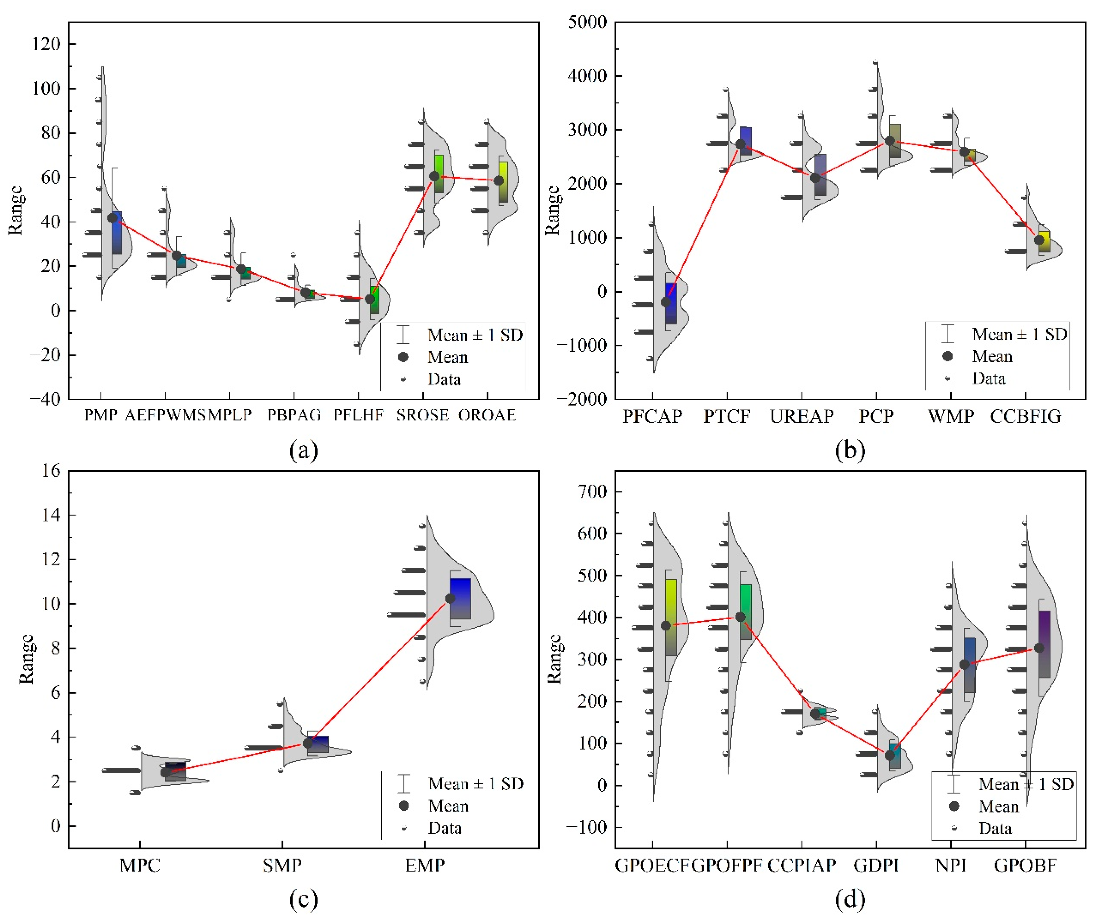
- Comprehensive integration of multi-dimensional features. A systematic review of various external factors affecting corn market prices was conducted, including planting costs, port inventory, feed farming, deep processing enterprises, corn substitutes, freight, and economic indicators. These multi-dimensional features provide more comprehensive information input for the model.
- (2)
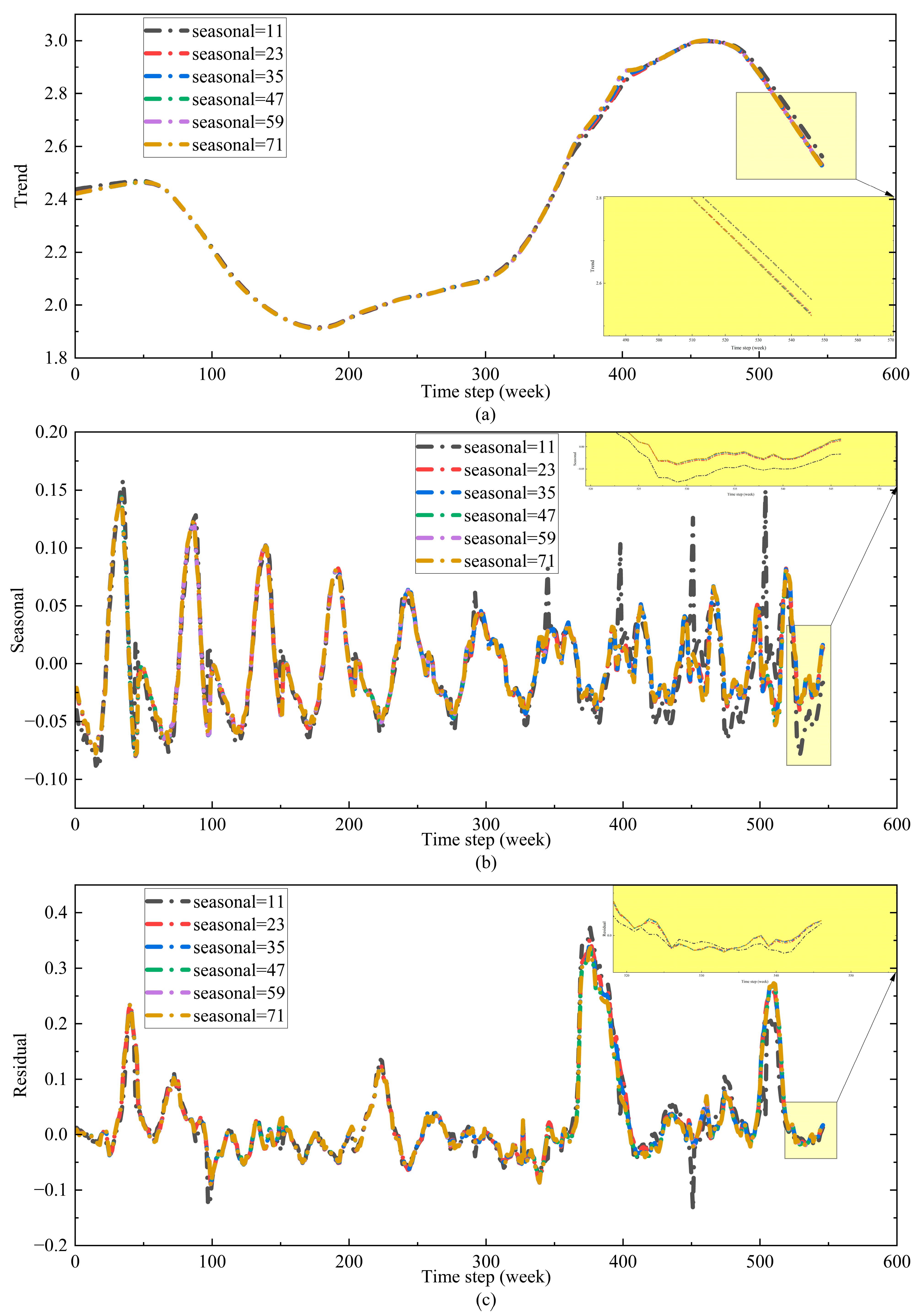
- In-depth mining of the complex price series volatility characteristics. The STL algorithm is used to extract the trend, seasonality, and residual components of the corn price series, and the GARCH-M model is combined to uncover the volatility clustering characteristics of the prices, integrating the inherent volatility patterns of the time series with external factors, significantly enhancing the model’s predictive ability.
- (3)
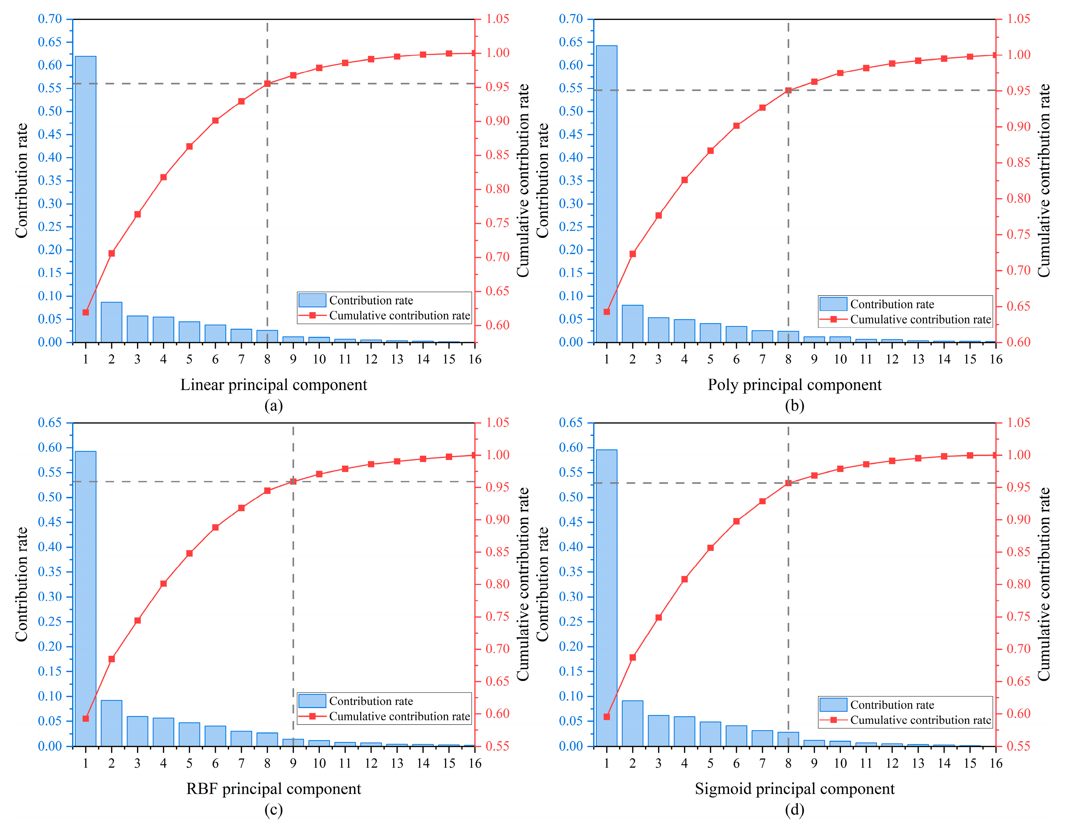
- Nonlinear dimensionality reduction and optimization of the model. KPCA was employed to reduce the dimensionality of the high-dimensional feature set, and a BiGRU-Attention model optimized by GWO was subsequently built. The model was optimized by automatically searching for key parameters, achieving high-precision predictions for corn market prices.
2. Materials and Methods
2.1. Factors Influencing Corn Market Price Fluctuations
2.2. GARCH-M
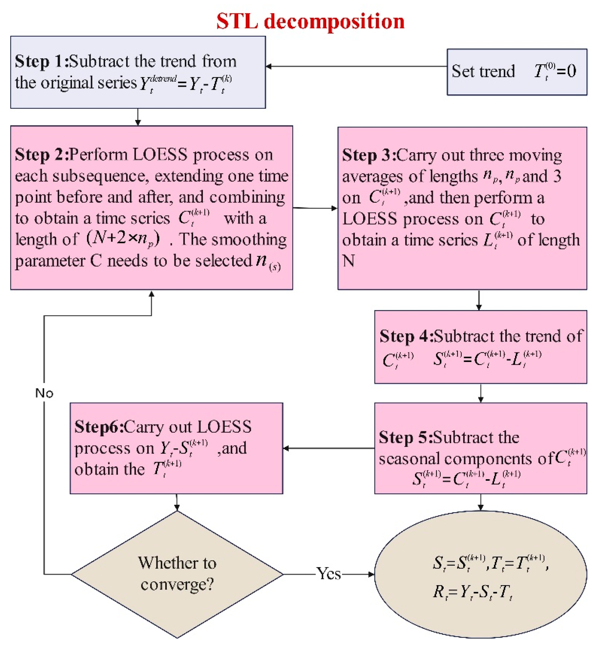
2.3. STL
2.4. KPCA
2.5. GWO
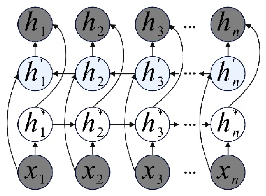
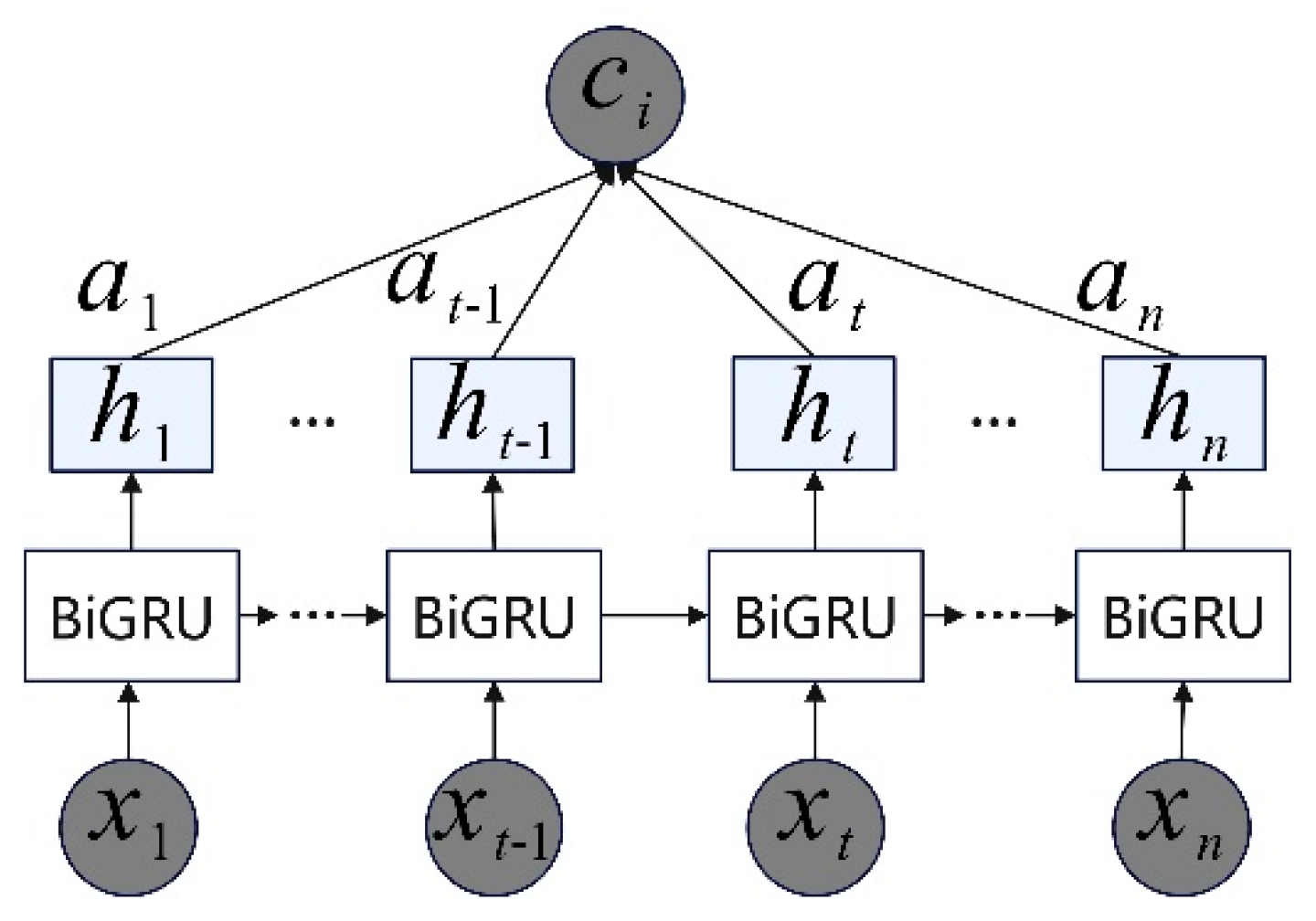
2.6. BiGRU-Attention
2.7. The Methodology
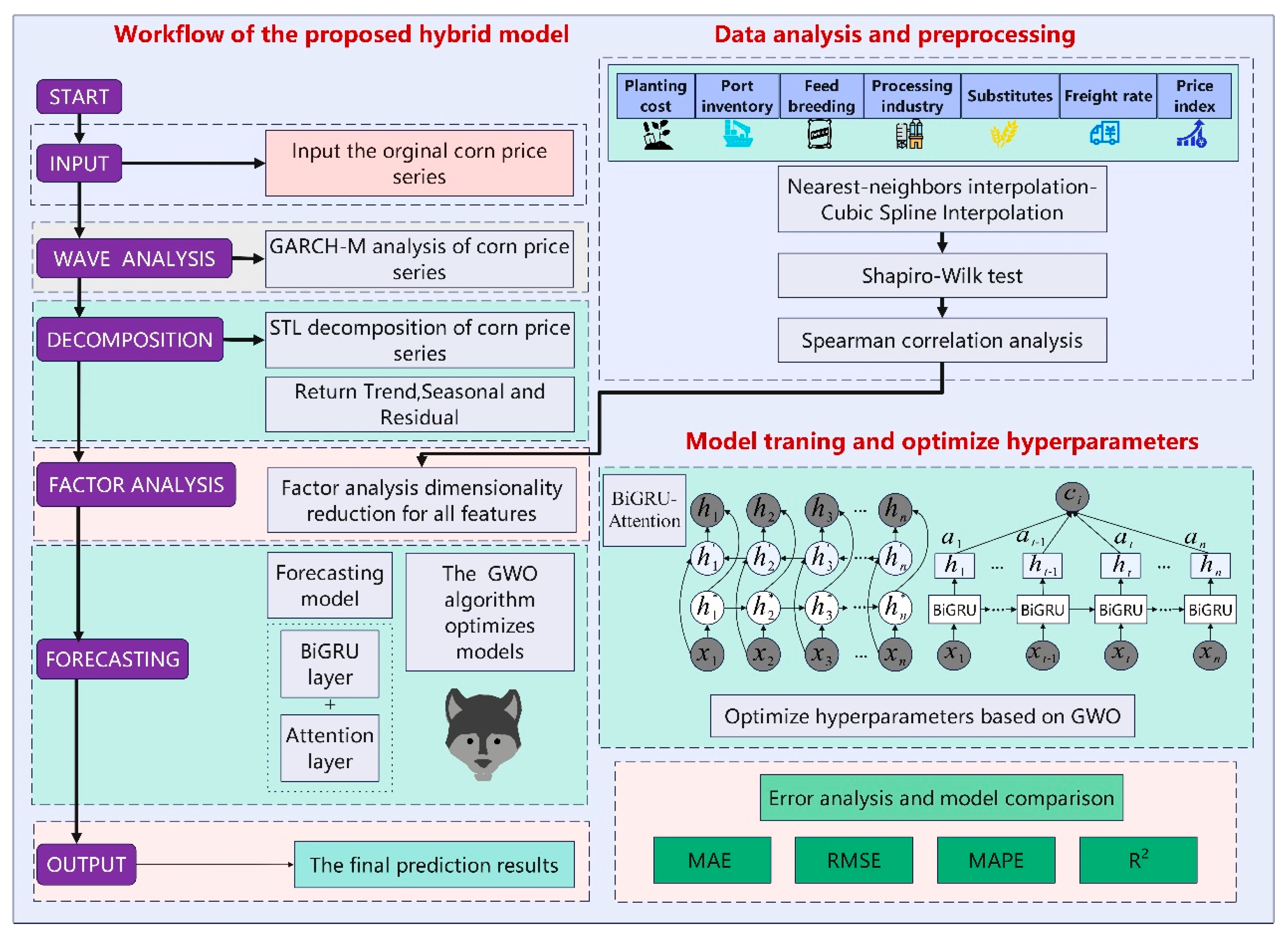
- (1)
- Data preprocessing: The acquired multi-factor data are temporally aligned based on the date dimension of the corn market price series. For missing values, a combined interpolation strategy using the nearest-neighbor interpolation method and cubic spline interpolation is employed.
- (2)
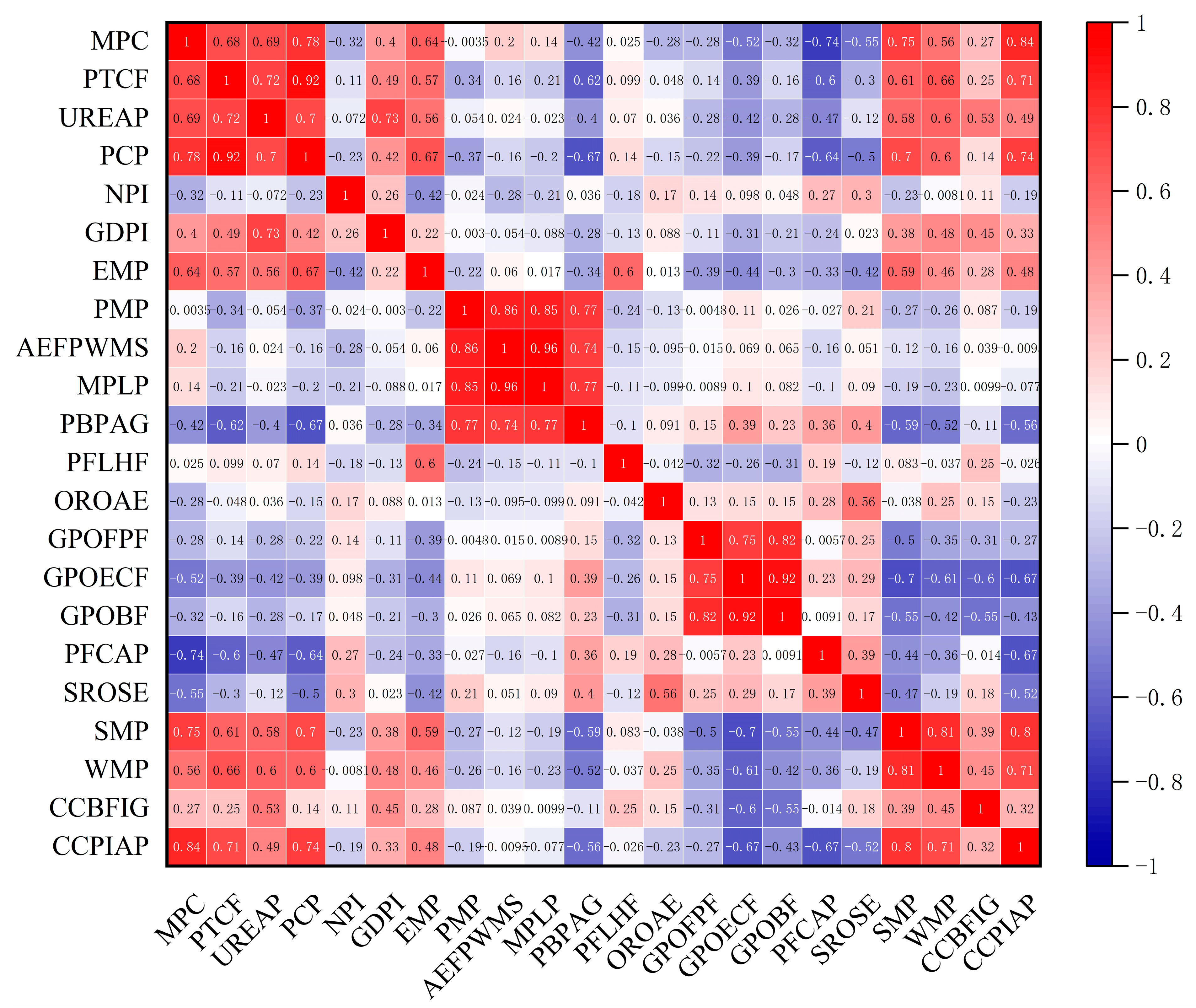
- Spearman’s rank correlation analysis: Spearman’s correlation analysis is applied to filter the key influencing factors of corn market prices. Before this, the Shapiro–Wilk test is applied to test the normality of the data.
- (3)
- Extraction of latent volatility information patterns and feature reduction: To allow the model to learn latent information patterns and enhance input information for better fitting, the GARCH-M and STL algorithms are employed to extract the complex fluctuation characteristics of the corn market price series and integrate them with external influencing factors, enhancing the model’s information expression. This paper uses KPCA to reduce the dimensionality of the constructed input feature matrix. In the GARCH-M model, the conditional mean equation and the variance equation are formulated, and the resulting volatility clustering feature is labeled as . Next, STL is used to obtain component information, which is divided into two steps: the inner and outer loops. Assume that and are the trends and seasonal components at the end of the th pass in the inner loop, with an initial condition of , and the parameters are , , , , , and .
- (4)
- GWO: The dimension-reduced corn price feature data are input into the BiGRU. In this paper, GWO is used to optimize the key parameters of the attention-based BiGRU model. The GWO algorithm continuously adjusts these parameters during training, searching for the optimal solution to improve model performance.
- (5)
- Prediction: The optimal solution parameters obtained are used as the new model parameters for training. The model is then tested on the test set to obtain the final predicted value . The evaluation metrics MAE, RMSE, MAPE, and R2 are computed by comparing the predicted value with the true value .
3. Analysis and Discussion of Experimental Results
3.1. Data Source
3.2. Data Preprocessing
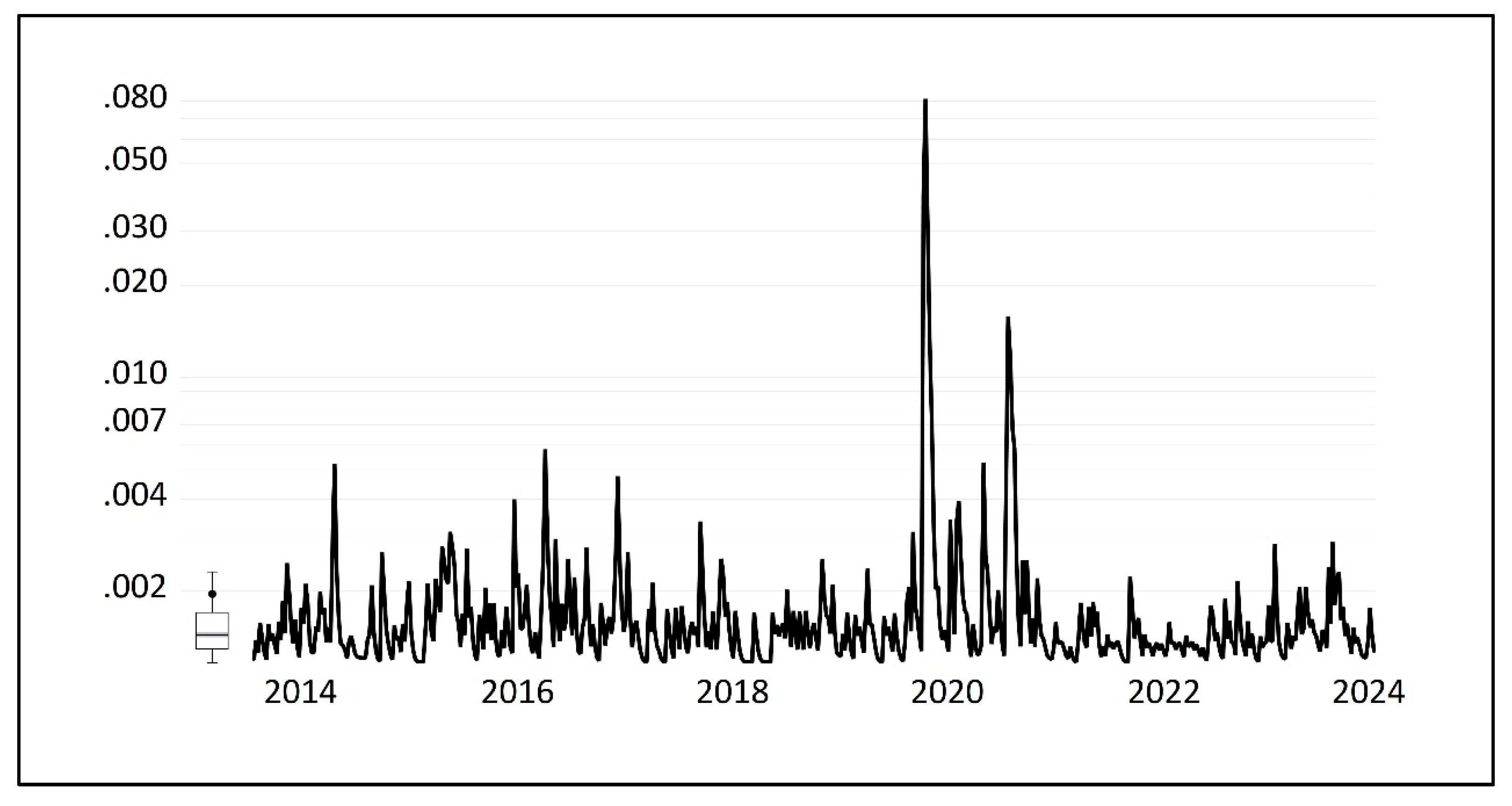
3.3. Extraction of Volatility Clustering Characteristics Using the GARCH-M Model
- (1)
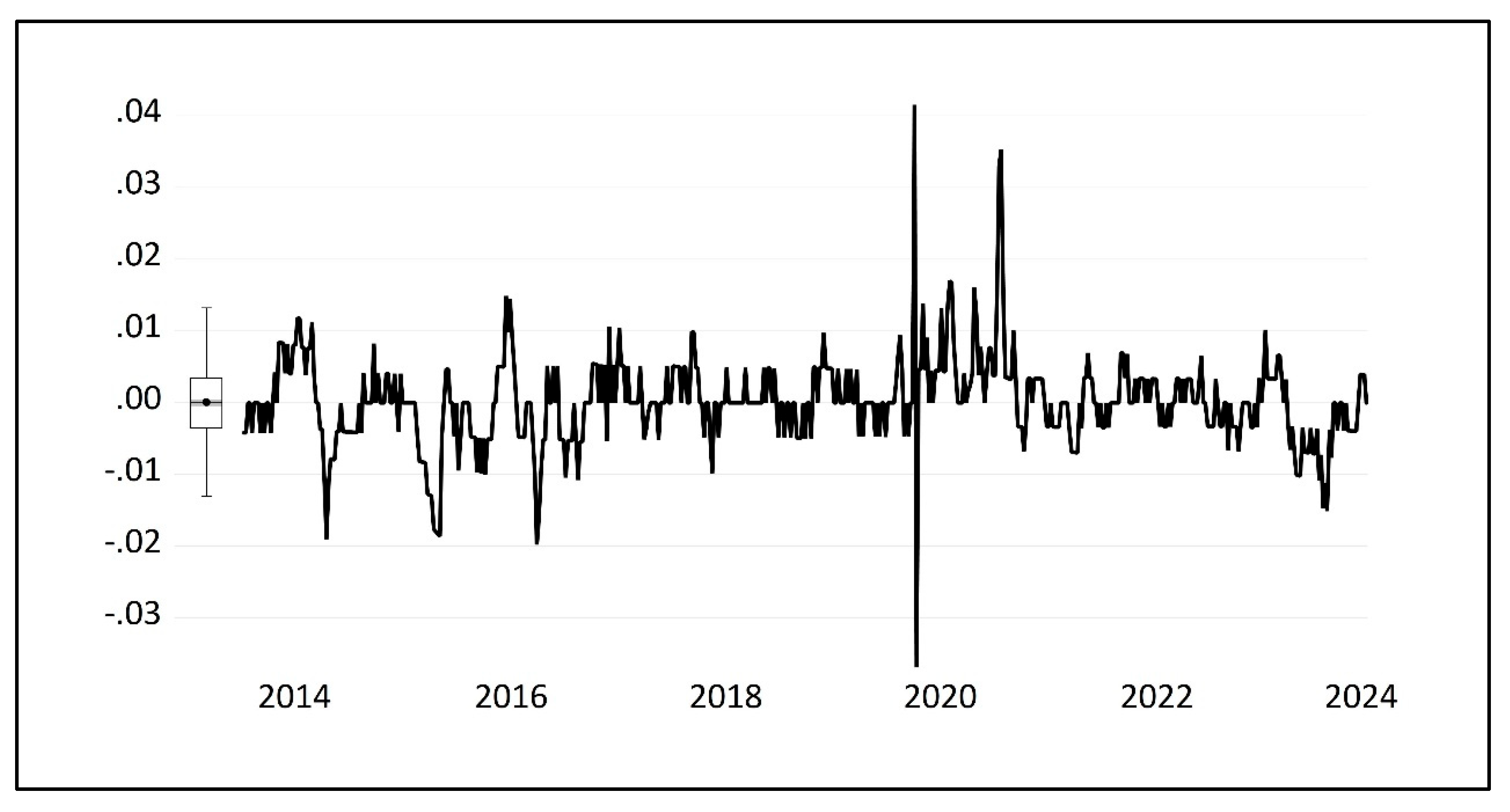
- Normality test and descriptive statistics of corn market price returns
- (2)
- Stationarity Test of the Return Series
- (3)
- Determining the Lag Order of the Conditional Mean Equation
- (4)
- ARCH Effect Test
- (5)
- Determination of Optimal Lag Order for the GARCH-M Model
3.4. Corn Market Price Feature Extraction Based on STL Decomposition
3.5. Performance Evaluation Metrics and Model Parameter Settings
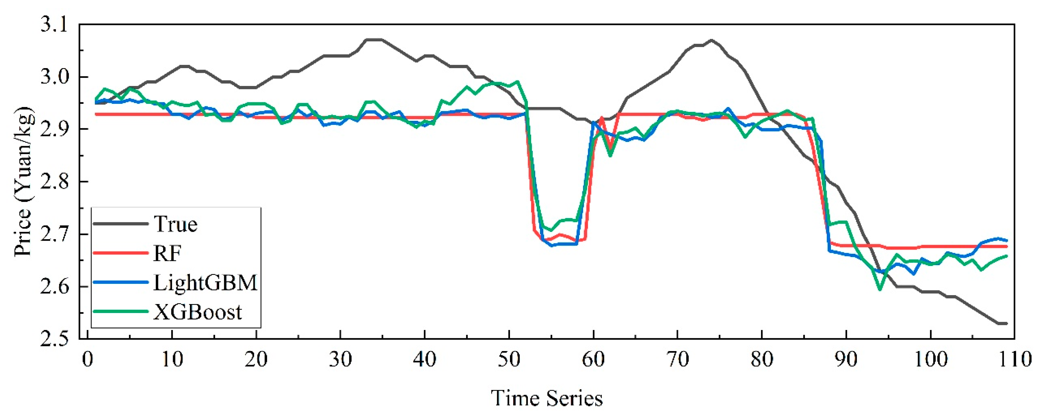
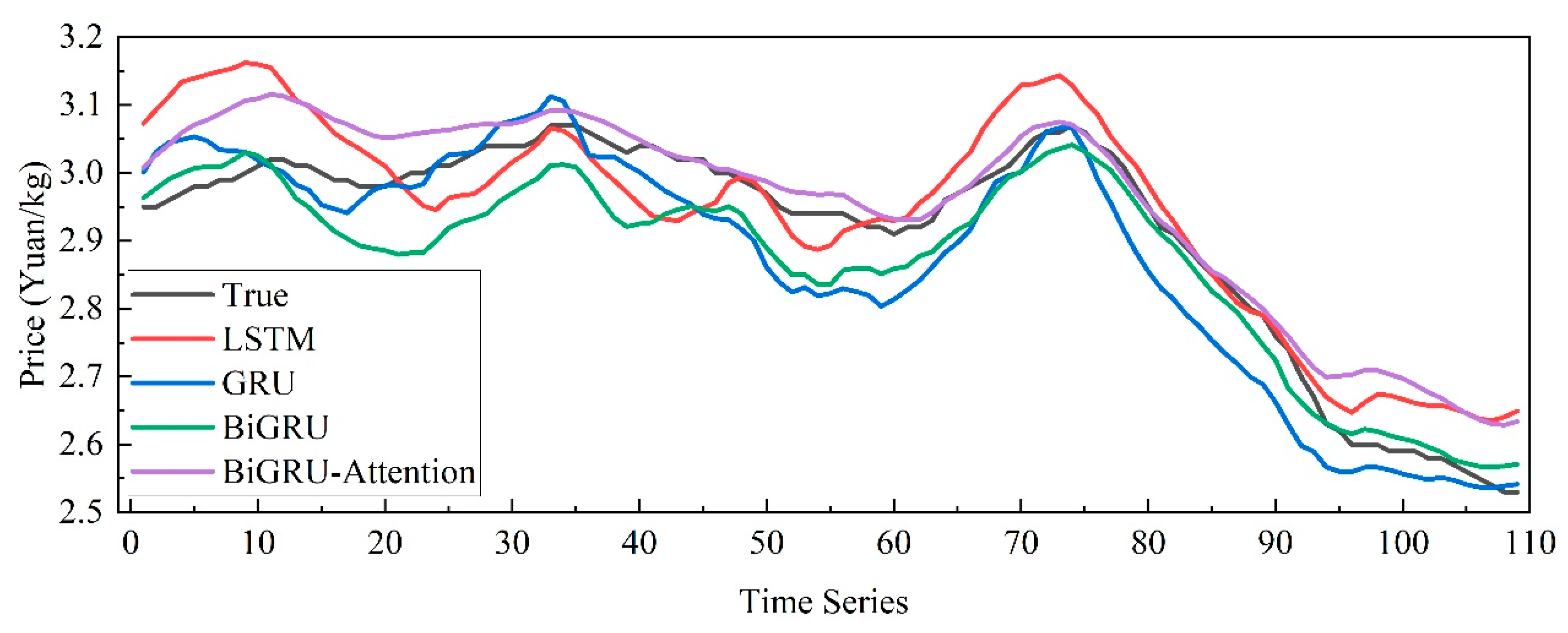
3.6. Cross-Sectional Forecasting with Multiple Influencing Factors
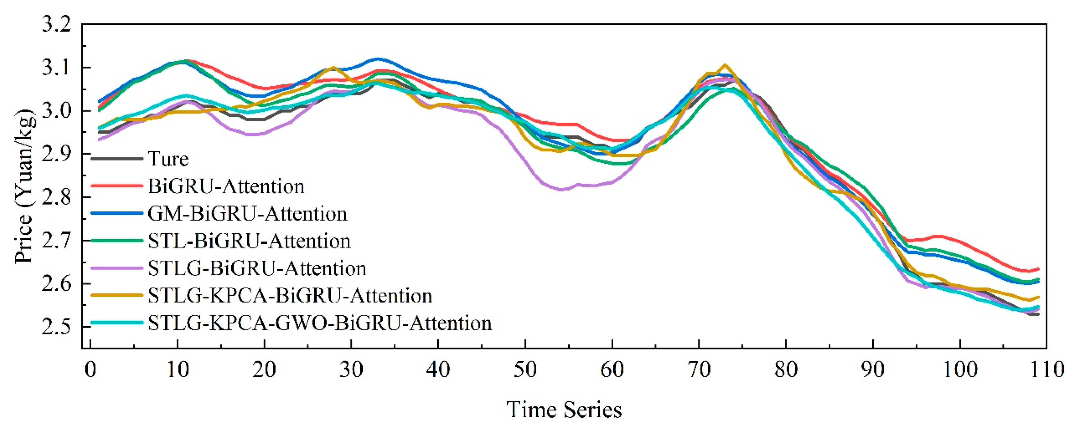
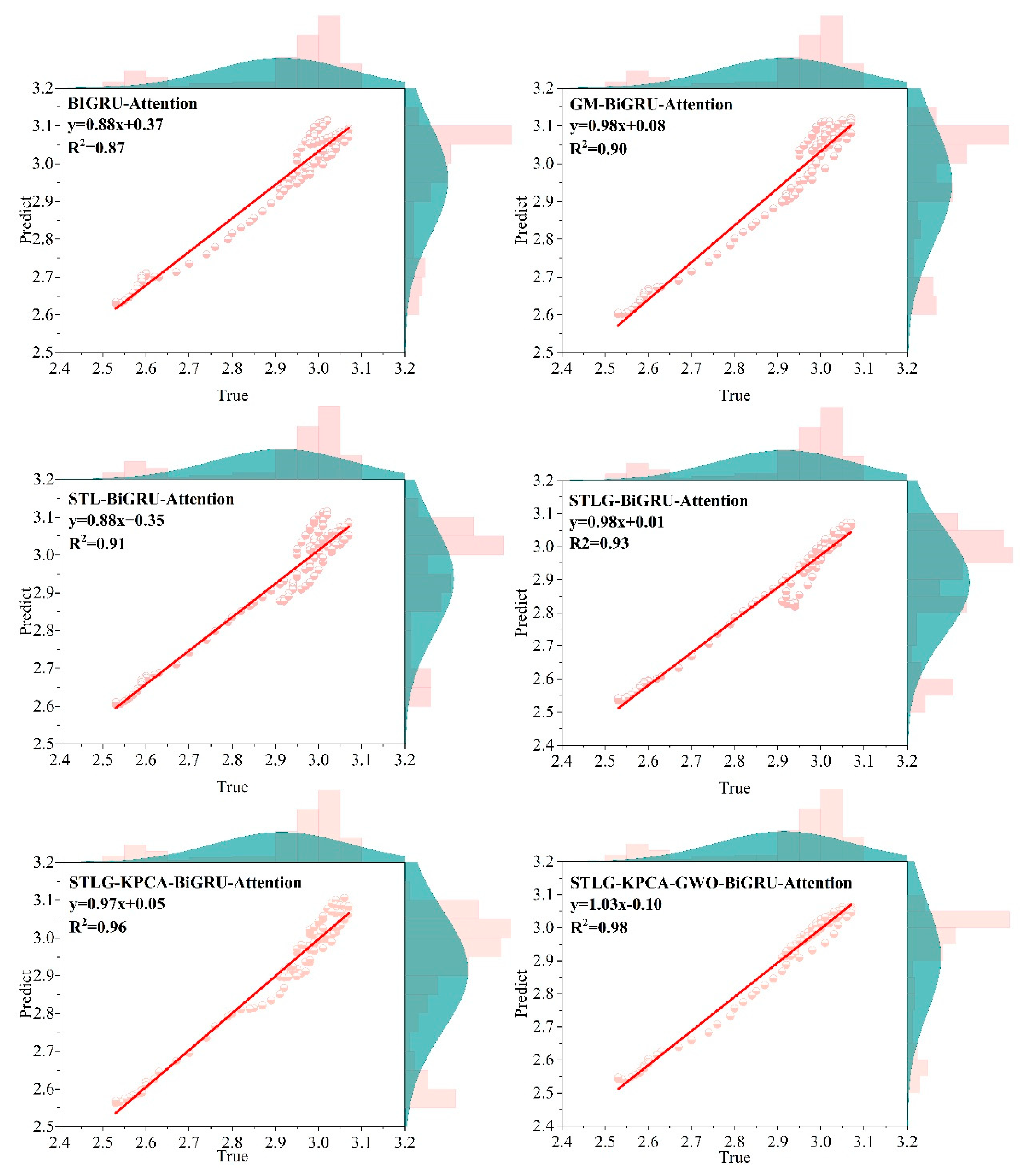
3.7. Longitudinal Forecasting with Multi-Feature Fusion and Grey Wolf Optimization
4. Conclusions
Author Contributions
Funding
Institutional Review Board Statement
Data Availability Statement
Conflicts of Interest
References
- Kyriazi, F.; Thomakos, D.D.; Guerard, J.B. Adaptive learning forecasting, with applications in forecasting agricultural prices. Int. J. Forecast. 2019, 35, 1356–1369. [Google Scholar] [CrossRef]
- Avinash, G.; Ramasubramanian, V.; Ray, M.; Paul, R.K.; Godara, S.; Nayak, G.H.; Kumar, R.R.; Manjunatha, B.; Dahiya, S.; Iquebal, M.A. Hidden Markov guided Deep Learning models for forecasting highly volatile agricultural commodity prices. Appl. Soft Comput. 2024, 158, 111557. [Google Scholar] [CrossRef]
- Sun, M.; Li, S.; Yang, W.; Zhao, B.; Wang, Y.; Liu, X. Commercial genetically modified corn and soybean are poised following pilot planting in China. Mol. Plant 2024, 17, 519–521. [Google Scholar] [CrossRef]
- Sun, Q.; Li, Y.; Gong, D.; Hu, A.; Zhong, W.; Zhao, H.; Ning, Q.; Tan, Z.; Liang, K.; Mu, L. A NAC-EXPANSIN module enhances maize kernel size by controlling nucellus elimination. Nat. Commun. 2022, 13, 5708. [Google Scholar] [CrossRef]
- Mu, W.; Kleter, G.A.; Bouzembrak, Y.; Dupouy, E.; Frewer, L.J.; Radwan Al Natour, F.N.; Marvin, H. Making food systems more resilient to food safety risks by including artificial intelligence, big data, and internet of things into food safety early warning and emerging risk identification tools. Compr. Rev. Food Sci. Food Saf. 2024, 23, e13296. [Google Scholar] [CrossRef]
- Wang, J.; Wang, Z.; Li, X.; Zhou, H. Artificial bee colony-based combination approach to forecasting agricultural commodity prices. Int. J. Forecast. 2022, 38, 21–34. [Google Scholar] [CrossRef]
- Zeng, L.; Ling, L.; Zhang, D.; Jiang, W. Optimal forecast combination based on PSO-CS approach for daily agricultural future prices forecasting. Appl. Soft Comput. 2023, 132, 109833. [Google Scholar] [CrossRef]
- Mohsin, M.; Jamaani, F. A novel deep-learning technique for forecasting oil price volatility using historical prices of five precious metals in context of green financing—A comparison of deep learning, machine learning, and statistical models. Resour. Policy 2023, 86, 104216. [Google Scholar] [CrossRef]
- Khadka, R.; Chi, Y.N. Forecasting the Global Price of Corn: Unveiling Insights with SARIMA Modelling Amidst Geopolitical Events and Market Dynamics. Am. J. Appl. Stat. Econ. 2024, 3, 124–135. [Google Scholar] [CrossRef]
- Zhou, Z.; Zhang, Y.; Zhao, J. Research on Vegetable Pricing and Replenishment Based on Exponential Smoothing Model Prediction. Trans. Comput. Appl. Math. 2024, 4, 11–18. [Google Scholar]
- Kilian, L. How to construct monthly VAR proxies based on daily surprises in futures markets. J. Econ. Dyn. Control 2024, 168, 104966. [Google Scholar] [CrossRef]
- Hassoo, A.K. Forecasting Maize Production In Romania: A BSTS Model Approach. Rom. Stat. Rev. 2024. [Google Scholar] [CrossRef]
- Caton, S.; Haas, C. Fairness in machine learning: A survey. ACM Comput. Surv. 2024, 56, 1–38. [Google Scholar] [CrossRef]
- Jin, B.; Xu, X. Forecasting wholesale prices of yellow corn through the Gaussian process regression. Neural Comput. Appl. 2024, 36, 8693–8710. [Google Scholar] [CrossRef]
- Xiang, X.; Xiao, J.; Wen, H.; Li, Z.; Huang, J. Prediction of landslide step-like displacement using factor preprocessing-based hybrid optimized SVR model in the Three Gorges Reservoir, China. Gondwana Res. 2024, 126, 289–304. [Google Scholar] [CrossRef]
- Liu, Z.L. Ensemble learning. In Artificial Intelligence for Engineers: Basics and Implementations; Springer: Cham, Switzerland, 2025; pp. 221–242. [Google Scholar]
- Zhao, Z.; Alzubaidi, L.; Zhang, J.; Duan, Y.; Gu, Y. A comparison review of transfer learning and self-supervised learning: Definitions, applications, advantages and limitations. Expert Syst. Appl. 2024, 242, 122807. [Google Scholar] [CrossRef]
- Murugesan, R.; Mishra, E.; Krishnan, A.H. Forecasting agricultural commodities prices using deep learning-based models: Basic LSTM, bi-LSTM, stacked LSTM, CNN LSTM, and convolutional LSTM. Int. J. Sustain. Agric. Manag. Inform. 2022, 8, 242–277. [Google Scholar] [CrossRef]
- Cheung, L.; Wang, Y.; Lau, A.S.; Chan, R.M. Using a novel clustered 3D-CNN model for improving crop future price prediction. Knowl. Based Syst. 2023, 260, 110133. [Google Scholar] [CrossRef]
- Wu, B.; Wang, Z.; Wang, L. Interpretable corn future price forecasting with multivariate time series. J. Forecast. 2024. [Google Scholar] [CrossRef]
- Wang, Y.; Wang, X.; Li, L. EMD-TCN-TimeGAN: A Data Augmentation Model for Enhancing the Accuracy of Agricultural Product Price Prediction. In Proceedings of the 2024 IEEE International Conference on Big Data (BigData), Washington, DC, USA, 15–18 December 2024; pp. 5161–5168. [Google Scholar]
- Ye, Z.; Zhai, X.; She, T.; Liu, X.; Hong, Y.; Wang, L.; Zhang, L.; Wang, Q. Winter Wheat Yield Prediction Based on the ASTGNN Model Coupled with Multi-Source Data. Agronomy 2024, 14, 2262. [Google Scholar] [CrossRef]
- Sun, F.; Meng, X.; Zhang, Y.; Wang, Y.; Jiang, H.; Liu, P. Agricultural Product Price Forecasting Methods: A Review. Agriculture 2023, 13, 1671. [Google Scholar] [CrossRef]
- Ray, S.; Lama, A.; Mishra, P.; Biswas, T.; Das, S.S.; Gurung, B. An ARIMA-LSTM model for predicting volatile agricultural price series with random forest technique. Appl. Soft Comput. 2023, 149, 110939. [Google Scholar] [CrossRef]
- Wang, D.; He, Z.; He, S.; Zhang, Z.; Zhang, Y. Dynamic pricing of two-dimensional extended warranty considering the impacts of product price fluctuations and repair learning. Reliab. Eng. Syst. Saf. 2021, 210, 107516. [Google Scholar] [CrossRef]
- Ge, Y.; Wu, H. Prediction of corn price fluctuation based on multiple linear regression analysis model under big data. Neural Comput. Appl. 2020, 32, 16843–16855. [Google Scholar] [CrossRef]
- Van Wesenbeeck, C.; Keyzer, M.; Van Veen, W.; Qiu, H. Can China’s overuse of fertilizer be reduced without threatening food security and farm incomes? Agric. Syst. 2021, 190, 103093. [Google Scholar] [CrossRef]
- Cao, Y.; Cheng, S. Impact of COVID-19 outbreak on multi-scale asymmetric spillovers between food and oil prices. Resour. Policy 2021, 74, 102364. [Google Scholar] [CrossRef]
- Yin, D.; Wang, Y.; Wang, L.; Wu, Y.; Bian, X.; Aggrey, S.E.; Yuan, J. Insights into the proteomic profile of newly harvested corn and metagenomic analysis of the broiler intestinal microbiota. J. Anim. Sci. Biotechnol. 2022, 13, 26. [Google Scholar] [CrossRef]
- Xu, Q.; Meng, T.; Sha, Y.; Jiang, X. Volatility in metallic resources prices in COVID-19 and financial Crises-2008: Evidence from global market. Resour. Policy 2022, 78, 102927. [Google Scholar] [CrossRef]
- Zeng, H.; Shao, B.; Dai, H.; Yan, Y.; Tian, N. Prediction of fluctuation loads based on GARCH family-CatBoost-CNNLSTM. Energy 2023, 263, 126125. [Google Scholar] [CrossRef]
- RB, C. STL: A seasonal-trend decomposition procedure based on loess. J. Off. Stat. 1990, 6, 3–73. [Google Scholar]
- Schölkopf, B.; Smola, A.; Müller, K.-R. Nonlinear component analysis as a kernel eigenvalue problem. Neural Comput. 1998, 10, 1299–1319. [Google Scholar] [CrossRef]
- Gong, R.; Li, X. A short-term load forecasting model based on crisscross grey wolf optimizer and dual-stage attention mechanism. Energies 2023, 16, 2878. [Google Scholar] [CrossRef]
- Tang, J.; Hou, H.; Chen, H.; Wang, S.; Sheng, G.; Jiang, C. Concentration prediction method based on Seq2Seg network improved by BI-GRU for dissolved gas intransformer oil. Electr. Power Autom. Equip. 2022, 42, 196–202. [Google Scholar]
- Xu, X.; Zhang, Y. Corn cash price forecasting with neural networks. Comput. Electron. Agric. 2021, 184, 106120. [Google Scholar] [CrossRef]


| Data Category | Name | Unit | Description |
|---|---|---|---|
| Target Variable | MPC | Yuan/kg | Corn market price |
| Planting Cost | PTCF | Yuan/t | Fertilizer price |
| UREAP | Yuan/t | Fertilizer price | |
| PCP | Yuan/t | Fertilizer price | |
| Port Inventory | NPI | Mt | Northern port inventory |
| GDPI | Mt | Guangdong port inventory | |
| Feed Farming | EMP | Yuan/kg | Egg market price |
| PMP | Yuan/kg | Piglet wholesale market price | |
| AEFPWMS | Yuan/kg | Average carcass price | |
| MPLP | Yuan/kg | Live pig exit price | |
| PBPAG | - | Pig-to-grain price ratio | |
| PFLHF | Yuan/100 | Profit from layer hen farming | |
| GPOFPF | Yuan/t | Gross profit of fattening pig feed | |
| GPOECF | Yuan/t | Gross profit of layer feed | |
| GPOBF | Yuan/t | Gross profit of broiler feed | |
| Enterprises | SROSE | % | Starch enterprise operating rate |
| PFCAP | Yuan/t | Corn ethanol processing profit | |
| OROAE | % | Alcohol enterprise operating rate | |
| Substitutes | SMP | Yuan/kg | Soybean meal price |
| WMP | Yuan/t | Wheat market price | |
| Freight Rate | CCBFIG | - | CCBFI: grain index |
| Price Index | CCPIAP | - | Economic indicators |
| t-Statistic | p-Value | |
|---|---|---|
| ADF test statistic | −8.048156 | 0.0000 |
| 1% significance level | −2.569228 | - |
| 5% significance level | −1.941407 | - |
| 1% significance level | −1.616307 | - |
| Statistical Values | p-Value | |
|---|---|---|
| F-statistic | 0.078003 | 0.7801 |
| Obs*R-squared | 0.078425 | 0.7794 |
| Statistical Values | p-Value | |
|---|---|---|
| F-statistic | 16.20240 | 0.0000 |
| Obs*R-squared | 135.7961 | 0.0000 |
| Error Distribution | (q,p,r) | AIC | SC | HQ |
|---|---|---|---|---|
| Student’s t | (3,3,0) | −8.249501 | −8.162451 | −8.215464 |
| Student’s t | (3,2,0) | −8.250523 | −8.171387 | −8.219581 |
| Student’s t | (3,1,0) | −8.249372 | −8.178149 | −8.221524 |
| Student’s t | (2,3,0) | −8.251125 | −8.171989 | −8.220183 |
| Student’s t | (2,2,0) | −8.253129 | −8.181906 | −8.225280 |
| Student’s t | (2,1,0) | −8.253046 | −8.189736 | −8.228292 |
| Student’s t | (1,3,0) | −8.253277 | −8.182054 | −8.225429 |
| Student’s t | (1,2,0) | −8.253092 | −8.189783 | −8.228338 |
| Student’s t | (1,1,0) | −8.256576 * | −8.201180 * | −8.234916 * |
| GED | (3,3,0) | −8.225419 | −8.138369 | −8.191382 |
| GED | (3,2,0) | −8.212415 | −8.133279 | −8.181473 |
| GED | (3,1,0) | −8.215526 | −8.144304 | −8.187678 |
| GED | (2,3,0) | −8.210055 | −8.130919 | −8.179113 |
| GED | (2,2,0) | −8.209535 | −8.138312 | −8.181687 |
| GED | (2,1,0) | −8.214488 | −8.151179 | −8.189734 |
| GED | (1,3,0) | −8.209567 | −8.138345 | −8.181719 |
| GED | (1,2,0) | −8.212434 | −8.149125 | −8.187680 |
| GED | (1,1,0) | −8.212317 | −8.156921 | −8.190657 |
| Parameter | Value | Explanation |
|---|---|---|
| period | 53 | Based on periodic characteristics of time series |
| low_pass | 55 | The smallest odd number greater than the period |
| seasonal | {11, 23, 35, 47, 59, 71} | Generally required to be an odd number no than 7 |
| robust | True | Perform robust decomposition |
| seasonal_jump | 1 | Not exceeding 10–20% of the seasonal and low_pass |
| trend_jump | 1 | Not exceeding 10–20% of the seasonal and low_pass |
| low_pass_jump | 1 | Not exceeding 10–20% of the seasonal and low_pass |
| Model | Hyperparameter Settings |
|---|---|
| RF | n_estimators = 100, max_depth = 5, random_state = 1, max_leaf_nodes = 10 |
| LightGBM | num_leaves = 31, learning_rate = 0.1, max_depth = 10 |
| XGBoost | n_estimators = 300, learning_rate = 0.2, max_depth = 2, min_child_weight = 1 |
| LSTM | lstm_units = 64, batch_size = 16, epochs = 100, activation function = relu, optimizer = adam |
| GRU | gru_units = 128, batch_size = 16, epochs = 100, activation function = relu, optimizer = adam |
| BiGRU | bigru_units = 128, batch_size = 16, epochs = 100, activation function = relu, optimizer = adam |
| BiGRU-Attention | bigru_units = 128, batch_size = 16, epochs = 100, activation function = relu, optimizer = adam, att activation function = sigmoid |
| Model | MAE | RMSE | MAPE (%) | R2 |
|---|---|---|---|---|
| RF | 0.0926 | 0.1066 | 3.2034 | 0.6129 |
| LightGBM | 0.0897 | 0.1041 | 3.0980 | 0.6306 |
| XGBoost | 0.0803 | 0.0937 | 2.7681 | 0.7011 |
| LSTM | 0.0578 | 0.0726 | 1.9507 | 0.7893 |
| GRU | 0.0534 | 0.0643 | 1.8796 | 0.8351 |
| BiGRU | 0.0508 | 0.0599 | 1.7592 | 0.8566 |
| BiGRU-Attention | 0.0433 | 0.0569 | 1.4884 | 0.8708 |
| Model | MAE | RMSE | MAPE (%) | R2 |
|---|---|---|---|---|
| BiGRU-Attention | 0.0433 | 0.0569 | 1.4884 | 0.8708 |
| GM-BiGRU-Attention | 0.0399 | 0.0493 | 1.3543 | 0.9027 |
| STL-BiGRU-Attention | 0.0382 | 0.0470 | 1.3197 | 0.9118 |
| STLG-BiGRU-Attention | 0.0265 | 0.0395 | 0.9241 | 0.9376 |
| STLG-KPCA-BiGRU-Attention | 0.0225 | 0.0279 | 0.7689 | 0.9687 |
| STLG-KPCA-GWO-BiGRU-Attention | 0.0159 | 0.0215 | 0.5544 | 0.9815 |
Disclaimer/Publisher’s Note: The statements, opinions and data contained in all publications are solely those of the individual author(s) and contributor(s) and not of MDPI and/or the editor(s). MDPI and/or the editor(s) disclaim responsibility for any injury to people or property resulting from any ideas, methods, instructions or products referred to in the content. |
© 2025 by the authors. Licensee MDPI, Basel, Switzerland. This article is an open access article distributed under the terms and conditions of the Creative Commons Attribution (CC BY) license (https://creativecommons.org/licenses/by/4.0/).
Share and Cite
Feng, Y.; Hu, X.; Hou, S.; Guo, Y. A Novel BiGRU-Attention Model for Predicting Corn Market Prices Based on Multi-Feature Fusion and Grey Wolf Optimization. Agriculture 2025, 15, 469. https://doi.org/10.3390/agriculture15050469
Feng Y, Hu X, Hou S, Guo Y. A Novel BiGRU-Attention Model for Predicting Corn Market Prices Based on Multi-Feature Fusion and Grey Wolf Optimization. Agriculture. 2025; 15(5):469. https://doi.org/10.3390/agriculture15050469
Chicago/Turabian StyleFeng, Yang, Xiaonan Hu, Songsong Hou, and Yan Guo. 2025. "A Novel BiGRU-Attention Model for Predicting Corn Market Prices Based on Multi-Feature Fusion and Grey Wolf Optimization" Agriculture 15, no. 5: 469. https://doi.org/10.3390/agriculture15050469
APA StyleFeng, Y., Hu, X., Hou, S., & Guo, Y. (2025). A Novel BiGRU-Attention Model for Predicting Corn Market Prices Based on Multi-Feature Fusion and Grey Wolf Optimization. Agriculture, 15(5), 469. https://doi.org/10.3390/agriculture15050469