Article

A Comparative Study of Neural Network Models for China’s Soybean Futures Price Forecasting

1
Agricultural Information Institute, Chinese Academy of Agricultural Sciences, Beijing 100081, China
2
Key Laboratory of Agricultural Big Data, Ministry of Agriculture and Rural Affairs, Beijing 100081, China
*
Author to whom correspondence should be addressed.
Agriculture 2025, 15(24), 2586; https://doi.org/10.3390/agriculture15242586
Submission received: 25 September 2025 / Revised: 30 November 2025 / Accepted: 3 December 2025 / Published: 15 December 2025
(This article belongs to the Section Agricultural Economics, Policies and Rural Management)

Abstract

Accurate prediction of soybean futures prices is crucial for agricultural risk management and market decision-making. This study systematically evaluated nine state-of-the-art deep learning models—iTransformer, TFT, TCN, TimesNet, PatchTST, TiDE, TSMixer, SOFTS, and Time-LLM—for forecasting the DCE No. 2 soybean futures price, while also examining the impact of incorporating external market variables (USFP, ER, SF). The results demonstrate that in univariate forecasting, iTransformer achieved the lowest MAPE over short (5–10 days) and long (60 days) horizons, while TCN demonstrated the most stable performance at the medium-term horizon (30 days); TimesNet attained the best RMSE, making it more suitable for handling extreme volatility and controlling tail errors. Under multivariate settings (with the introduction of USFP, ER, and SF as exogenous variables), TFT demonstrates the best overall performance, significantly outperforming the LSTM baseline model across nearly all forecast horizons. The gains from exogenous variables depend on both the forecast horizon and the choice of covariates. These findings provide empirical guidance for participants in futures markets regarding model selection and covariate configuration, supporting more precise risk management and market decision-making.

1. Introduction

Soybeans serve as both an essential food crop and a major oilseed, and their by-product, soybean meal, is a critical protein source for China’s livestock sector, particularly in swine feed [1]. In recent years, driven by economic growth and evolving dietary patterns, China’s soybean demand has continued to rise [2], with the country remaining highly dependent on international markets. According to data from the General Administration of Customs of China (GACC), China imported 105 million tons of soybeans in 2024, corresponding to an import-dependence ratio of 83.57% [3,4]. Under these conditions, China’s soybean market is highly vulnerable to external shocks such as geopolitical tensions, trade policy adjustments, extreme weather events, and exchange rate fluctuations [5]. These shocks often trigger domestic price volatility, which is then transmitted along the supply chain, affecting soybean meal availability, feed processing, livestock production, and broader food-security outcomes [6,7,8]. In the face of frequent external shocks and increasing price volatility, futures markets play a particularly important role in price discovery and risk management. Through open and competitive trading mechanisms, futures markets generate forward-looking price signals and provide effective hedging instruments that help producers, processors, traders, and investors manage market uncertainty [9,10,11,12,13]. Since the launch of soybean futures trading on the Dalian Commodity Exchange (DCE) in 1993, DCE soybean futures prices have become key benchmarks for pricing and information transmission throughout China’s soybean supply chain [14]. Accurate forecasting of soybean futures prices is therefore essential for improving risk management, procurement planning, and market monitoring.
As a variable with the dual attributes of financial time-series data and agricultural commodities, soybean futures prices exhibit seasonality, stochastic volatility, and nonlinearity [15,16,17]. Traditional time-series models rely on the assumption of stationarity in the data and struggle to handle complex nonlinear relationships [18]. Consequently, relying solely on conventional statistical models may lead to suboptimal forecasts and limit their usefulness in real-world decision-making [19]. With the rapid development of artificial intelligence, machine learning (ML) and deep learning (DL), which offer powerful high-dimensional feature extraction and nonlinear modeling capabilities, have become the main tools in financial price forecasting. In particular, deep-learning neural networks excel at handling noisy, highly chaotic time-series data, mitigate overfitting more effectively, and offer stronger generalization, making them a primary focus of current research [20,21]. For example, the Sample Convolution and Interaction Network (SCINet) has shown strong results in multi-step corn price prediction, while hybrid models such as the Convolutional Neural Network and Long Short-Term Memory mode l (CNN-LSTM) based on the Bayesian optimization (BO) algorithm (BO-CNN-LSTM), and transformer-based frameworks like Patch Time Series Transformer (PatchTST) and iTransformer, have demonstrated superior accuracy and robustness in forecasting soybean and soybean-meal futures [11,15,18,22,23]. Overall, no single neural network model is uniformly optimal across all futures contracts. Hybrid-model–based forecasting generally outperforms single-model approaches. Incorporating appropriate exogenous variables effectively enhances predictive performance [24]. The reasons for this are twofold: (1) different futures contracts, especially different agricultural futures, differ markedly in statistical properties and driving factors; and (2) neural network models vary in their emphases on memory horizon, seasonality/trend representation, integration of exogenous variables, probabilistic modeling, and computational efficiency. Therefore, it is necessary to systematically evaluate model performance for specific contracts in order to identify the most suitable architecture and provide precise tools for practical trading and risk management.
Soybean futures price forecasting has been extensively studied using neural networks. As Table 1 illustrates, neural network-based models underpin 12 of the 14 reviewed studies. Recurrent architectures such as RNN, LSTM, GRU, and Attention-LSTM remain the most commonly used, while several studies investigate hybrid CNN-LSTM models or complex decomposition–forecasting pipelines including EEMD-NAGU and ICEEMDAN-LZ-BVMD-SSA-DELM. Although these approaches have produced many valuable results, prior studies have also identified several inherent limitations. These include difficulties in modeling long-range dependencies, limited ability to capture multiscale temporal structures, and insufficient mechanisms for effectively incorporating nonlinear exogenous covariates [25,26]. In addition, decomposition-based hybrid models typically rely on multi-stage procedures, which not only increase computational burden but may also reduce robustness due to the propagation of decomposition errors across stages. These limitations are particularly relevant for agricultural futures, which typically exhibit long-horizon dependence, multiscale volatility characteristics, and strong exogenous influences. In recent years, newer architectures such as Time-LLM, TSMixer, SOFTS, and TiDE have demonstrated strong performance according to general time-series benchmarks, yet their potential strengths in long-horizon forecasting, efficient representation learning, and multivariate joint modeling have not been systematically evaluated in agricultural futures markets. Therefore, this study selects nine representative state-of-the-art models to conduct a consistent and comprehensive comparative assessment tailored to the forecasting characteristics of agricultural futures, thereby addressing the methodological gap in this field.
China’s soybean futures market features a dual-contract system. The No. 1 contract, grounded in domestic non-GM food soybeans, serves the food processing industry, while the No. 2 contract, tied to imported GM soybeans, is priced in direct linkage with the global market [38]. Although academic focus has historically been on the more liquid No. 1 contract, which has yielded substantial findings in price discovery [39,40,41], volatility transmission [42,43], and price forecasting [9,11,16,28], studies reveal that the No. 2 contract plays a disproportionately large role in price discovery [44], even outperforming its counterpart [45]. Given that the dominant position of U.S. soybeans in the global pricing system has been weakened in the context of U.S.–China trade frictions [41], the necessity for systematic research on the No. 2 contract, which is directly integrated with international markets, is further underscored. Therefore, as the liquidity of the No. 2 contract improves, forecasting its prices is essential not only to fill a gap in the literature but also to safeguard national food security and stabilize the operations of related industrial chains.
Soybean futures prices are co-determined by multiple factors, including global supply–demand fundamentals, macroeconomic and financial conditions, trade and logistics costs, as well as external shocks such as geopolitical conflicts and extreme weather [27,29,37,46,47]. The price formation of the No. 2 soybean contract is more directly anchored in the “import cost” mechanism. Its key determinants are concentrated in three primary aspects: (1) the CBOT soybean futures price, which represents global supply–demand dynamics and serves as the benchmark price signal; (2) the USD/CNY exchange rate, which reflects the import cost in local currency terms; and (3) ocean freight costs, which capture international transportation expenses and trade competitiveness. These three variables collectively constitute the most core and rigid components of the No. 2 contract’s pricing system—a relationship that is both economically interpretable and empirically well-supported [27,46,48,49]. Furthermore, unlike factors such as geopolitical events or extreme weather that resist consistent quantification, these variables provide transparent, high-frequency data and exhibit characteristics suggestive of exogeneity, making them more amenable to integration into deep learning models and offering a solid foundation for enhancing the robustness and interpretability of multi-step forecasts. Their exogeneity and lead–lag relationships are further empirically examined through cross-correlation analysis, as detailed in Appendix A.
Considering the above context, the purpose of this study is to systematically evaluate the predictive performance of advanced deep learning models for China’s DCE No. 2 soybean futures price and to examine the role of exogenous variables in improving model accuracy. The main innovations and contributions of this study are threefold. First, this study fills a gap in the existing literature by focusing on the DCE No. 2 soybean futures contract, which is closely linked to China’s import-dependent market structure, in contrast to the extensively studied No. 1 contract. Second, this study introduces and compares multiple state-of-the-art deep learning models, expanding the application boundaries of such methods in agricultural futures price forecasting. Third, this study incorporates key exogenous variables such as U.S. soybean futures, exchange rates, and ocean freight costs, and quantitatively evaluates their incremental value in enhancing forecasting performance.
The research process includes three main stages:
  • Univariate forecasting: Under a fixed data split, we conduct a unified evaluation of Time-LLM, SOFTS, TiDE, iTransformer, PatchTST, TimesNet (Temporal 2D-Variation Modeling for General Time Series Analysis), TSMixerx, TCN, and TFT (Temporal Fusion Transformer), with the canonical recurrent neural network LSTM serving as the benchmark.
  • Single-target multivariate forecasting: We take the DCE No. 2 soybean futures price as the forecasting target. Using models capable of processing exogenous variables (namely TSMixer, TCN, TFT, TiDE, and LSTM), we build multivariate models to test whether incorporating these variables improves predictive performance.
  • Multi-step forecasting performance and robustness evaluation: We evaluate all models across varying forecast horizons to examine the robustness of their performance as the horizon changes. This analysis provides practical guidance for model selection across different decision cycles.
The structure of this paper is organized as follows: Section 1 introduces the research background, motivation, innovations, and objectives. Section 2 presents the methodology and data. Section 3 reports the empirical results from both univariate and multivariate forecasting experiments, followed by an evaluation of multi-step robustness across forecast horizons. Section 4 discusses the main findings, robustness verification, and practical implications, and further identifies the limitations of the study and directions for future research. Section 5 summarizes the results of the research.

2. Materials and Methods

2.1. Dataset Description

This study utilizes eight datasets across three categories: futures, exchange rates, and freight costs. Among them, the freight cost category includes five major soybean shipping routes from China’s three principal import origins (Brazil, the United States, and Argentina), which together account for approximately 96% of China’s total soybean imports [3]. These routes cover shipments from Santos (Brazil), Paranaguá (Brazil), Argentina, the U.S. Gulf Coast, and the U.S. Pacific Northwest to China. For simplicity, the freight cost variables derived from these routes are collectively referred to as SF in the subsequent analysis. The details of all variables, including abbreviations, descriptions, data sources, and descriptive statistics, are provided in Table 2 and Table 3, while their temporal dynamics are illustrated in Appendix B.1.

2.2. Data Preprocessing

This study constructs the raw futures price series using the contract with the largest open interest. To account for the non-overlapping public holidays between China and the U.S. and to maintain a continuous sequence of trading observations, non-trading days (weekends and holidays) were excluded based on the trading calendar of Chinese soybean futures. This ensures regular time steps required for deep learning model training and evaluation. Price movements on the first trading day following a non-trading period (e.g., Monday) inherently incorporate information and expectations accumulated during the preceding non-trading days; thus, potential jumps caused by macroeconomic announcements or policy events are reflected in subsequent observations rather than omitted. For missing values in exchange rates and shipping freight, they were supplemented using forward filling and linear regression fitting, respectively.
The sample period spans from 1 January 2007 to 31 December 2024, comprising 4365 valid records. The dataset was split chronologically, with the first 90% allocated to the training set and the remaining 10% reserved for validation and testing. All continuous features were normalized using the Robust Scaler, which rescales data based on the median and interquartile range (IQR) to mitigate the influence of outliers.
Specifically, the transformation is defined as
X = X Median ( X ) IQR ( X )
This approach enhances robustness against weak outliers and improves model convergence stability.
Before introducing the model architectures, the complete end-to-end workflow of the forecasting pipeline is illustrated in Figure 1. This diagram summarizes the procedures of data splitting, preprocessing, TPE-based hyperparameter optimization, model training, and performance evaluation.

2.3. Research Methods

This study selects nine representative models from five mainstream neural network architectures: MLP, CNN, Transformer, LLM, and RNN. The selected models include SOFTS, TiDE, TSMixerx, TCN, TimesNet, PatchTST, iTransformer, TFT, and Time-LLM. LSTM serves as a classical RNN benchmark model, providing the baseline for comparative evaluation. Each architecture embodies distinct modeling principles and strengths in capturing temporal dependencies and feature interactions, thereby offering a fair and diverse foundation for systematic comparison across representative neural forecasting paradigms.

2.3.1. MLP-Based Models

  • SOFTS
SOFTS is an efficient MLP-based model that streamlines the forecasting process and enhances prediction accuracy. SOFTS incorporates the STar Aggregate–Redistribute (STAR) module, which implements a centralized strategy that first aggregates information across channels to construct a global core representation and then redistributes it to individual channels for fusion, thereby enabling efficient cross-channel interaction [50]. By replacing distributed pairwise interactions with this centralized mechanism, STAR reduces the typical quadratic complexity to linear, substantially improving scalability and computational efficiency.
  • TiDE
TiDE is an encoder–decoder model architecture based on MLP, which comprises four core components: feature projection, dense encoder, dense decoder, and temporal decoder [18]. The dynamic covariates per time-point are mapped to a lower dimensional space using a feature projection step. Then the encoder combines the look-back along with the projected covariates with the static attributes to form an encoding. The decoder maps this encoding to a vector per time-step in the horizon. Then a temporal decoder combines this vector (per time-step) with the projected features of that time-step in the horizon to form the final predictions. We also add a global linear residual connection from the look-back to the horizon. The model retains both the simplicity and speed of linear models while effectively capturing nonlinear dependencies and incorporating covariate information [51].
  • TSMixer
TSMixer is based on mixing operations along both the time and feature dimensions to extract information efficiently. The time-domain MLPs are shared across all of the features, while the feature-domain MLPs are shared across all of the time steps. The interleaving design between these two operations efficiently utilizes both temporal dependencies and cross-variate information while limiting computational complexity and model size [52].

2.3.2. CNN-Based Models

  • TCN
TCN is a CNN-based architecture tailored for sequence data, particularly time series. It enforces causality via causal convolutions so that the output at time t depends only on inputs at t and earlier, thereby preventing any leakage of future information. Dilated convolutions expand the receptive field exponentially, enabling the model to capture long-range dependencies. While residual connections alleviate vanishing gradients, support deeper networks, and improve training stability [53].
  • TimesNet
Based on the multi-periodicity of time series, Wu et al. [25] proposed the TimesNet with a modular architecture to capture the temporal patterns derived from different periods. For each period, to capture the corresponding intraperiod and interperiod variations, a TimesBlock is designed within the TimesNet, which can transform the 1D time series into 2D space and simultaneously model the two types of variations by a parameter-efficient inception block. Thus, TimesNet can achieve a more effective representation learning than directly from 1D time series [25].

2.3.3. Transformer-Based Models

  • PatchTST
The Transformer has become a widely used architecture in modern deep learning. Nie [54] introduced PatchTST, an effective Transformer-based model design for time series forecasting tasks, by incorporating two key components: patching and a channel-independent structure. The Patch module segments the series into temporal patches using a chosen window size and stride. These patches are then fed to the Transformer, whose self-attention captures global dependencies among patches and thereby improves predictive performance [18]. This design enables the model to capture local semantic information and benefft from longer look-back windows [54].
  • iTransformer
iTransformer modifies none of the native components of the Transformer architecture. Instead, it simply applies the attention and feed-forward network to inverted dimensions. iTransformer regards independent series as variate tokens to capture multivariate correlations by attention and utilize layer normalization and feed-forward networks to learn series representations [55]. iTransformer enhances the Transformer family with promoted performance, stronger generalization across different variates, and better utilization of arbitrary lookback windows, making it a nice alternative as the fundamental backbone of time series forecasting.
  • TFT
TFT is an attention-based deep neural network (DNN) architecture [26,56]. As it retains the encoder–decoder backbone of the Transformer, this study categorizes it under the Transformer architecture. Lim [26] proposed the TFT architecture with the following key components: it accepts static metadata, time-varying past inputs, and time-varying a priori known future inputs as its input sources. Variable Selection is used for the judicious selection of the most salient features based on the input. Gated Residual Network blocks enable efficient information flow with skip connections and gating layers. Time-dependent processing is based on LSTMs for local processing, and multi-head attention for integrating information from any time step.

2.3.4. LLM-Based Models

Time-LLM is a reprogramming framework that adapts large language models (LLMs) for time-series forecasting while keeping the backbone unchanged [57]. The framework comprises three components: (1) patch tokenization of the input time series followed by a customized embedding layer; (2) cross-modal reprogramming of the patch embeddings using condensed textual prototypes, complemented by task-specific prompt prefixes that guide the transformation of the patches; and (3) a projection head that maps the LLM outputs back to the time-series domain to produce forecasts. Through this reprogramming approach, LLMs can act as effective few-shot and even zero-shot time series learners, outperforming specialized forecasting models.

2.4. Experimental Evaluation Metrics

Three main evaluation metrics were used to evaluate the model’s accuracy in this study, including mean absolute error (MAE), root mean square error (RMSE), and mean absolute percentage error (MAPE) calculated as
M A E = 1 n i = 1 n y i y ^ i
R M S E = 1 n i = 1 n y i y ^ i 2
M A P E = 1 n i = 1 n y i y ^ i y i × 100 %
where y i and y ^ i denote the observed and forecasted prices of Chinese soybean futures, respectively, and n is the number of observations in the out-of-sample period. Lower MAE, RMSE, and MAPE values indicate better model accuracy, with MAE being less affected by outliers, RMSE being particularly sensitive to large errors, and MAPE providing a relative error measure, making it suitable for comparison across different datasets [22].
To ensure consistency in model evaluation, this study specifies the ranking of performance criteria as follows: the primary criterion is the lowest MAPE, which measures forecast accuracy and allows comparison across different horizons; the secondary criterion is the RMSE, which reflects the variability of prediction errors; when models exhibit similar average MAPE values, the model with more stable performance is preferred.

2.5. Hyperparameter Optimization

Hyperparameter optimization was conducted using the Tree-structured Parzen Estimator (TPE) algorithm implemented in the HyperOpt library. The TPE method constructs a probabilistic surrogate model of the objective function based on historical evaluation results, allowing for adaptive exploration of the hyperparameter space and improving both search efficiency and model stability. Unlike traditional grid search or random search methods, TPE does not directly model the objective function f ( x ) . Instead, it estimates two probability density functions:
g x = p x y < y *
and
l x = p x y y *
where y * denotes a performance threshold (e.g., the top quantile of evaluation scores).
The algorithm then selects the next candidate hyperparameter configuration by maximizing the Expected Improvement (EI) criterion:
E I x = g ( x ) l ( x )
which measures the likelihood that a new configuration x will outperform the current best result.
During optimization, all models share a unified hyperparameter search space, with the MAE used as the optimization objective due to its robustness to outliers and stable gradient behavior. The detailed search ranges are summarized in Table A1 in Appendix B.2.
This probabilistic optimization strategy enables efficient exploration of high-dimensional hyperparameter spaces while maintaining low computational overhead, making it well-suited for deep learning forecasting models with complex parameter interactions.

2.6. Computational Setup

All experiments were conducted on a workstation equipped with two NVIDIA A100 GPUs (40 GB memory each), two Intel(R) Xeon(R) Gold 6132 CPUs (2.60 GHz), and 512 GB RAM. The software environment consisted of Python 3.10, PyTorch 2.5.1, Ray Tune 2.20, and CUDA 12.4. This configuration ensured adequate computational resources for efficient model training, hyperparameter optimization, and experimental reproducibility.

3. Results

3.1. Results: Univariate Forecasting

This study conducts time-series modeling based on the price data of China’s No. 2 soybeans futures contract. A systematic comparative analysis of nine advanced deep learning models reveals distinct differences in their aggregate performance throughout the forecasting horizon. As shown in Table 4, iTransformer, TimesNet, and SOFTS achieve the best overall performance on this dataset, significantly outperforming the LSTM baseline (MAE = 237.90, MAPE = 0.0653, RMSE = 264.09) across all three metrics. Specifically, iTransformer achieves the best MAE and MAPE, with reductions of 43.9% and 40.7%, respectively; its RMSE also secures a top result, exhibiting a 29.3% decrease relative to the LSTM baseline. Notably, TimesNet attains the best RMSE and demonstrates greater stability in capturing price spikes and large swings. SOFTS is close to optimal across all three metrics (MAE = 140.99, MAPE = 4.07%, RMSE = 187.85) and, as a lightweight MLP-based approach, is well suited to latency-sensitive inference scenarios.
In contrast, TFT records a significantly higher RMSE of 558.98, which is approximately three times that of iTransformer, TimesNet, and SOFTS. It exhibits weaker error control and limited robustness on samples with extreme volatility. Time-LLM performs substantially worse on all three metrics (MAE = 438.06, MAPE = 12.60%, RMSE = 505.67). This indicates that a minimal adaptation strategy for general-purpose LLMs [57], without dedicated time-series retraining, may be insufficient to achieve the performance level of models specifically designed for forecasting [58].

3.2. Results: Univariate Target with Exogenous Covariates

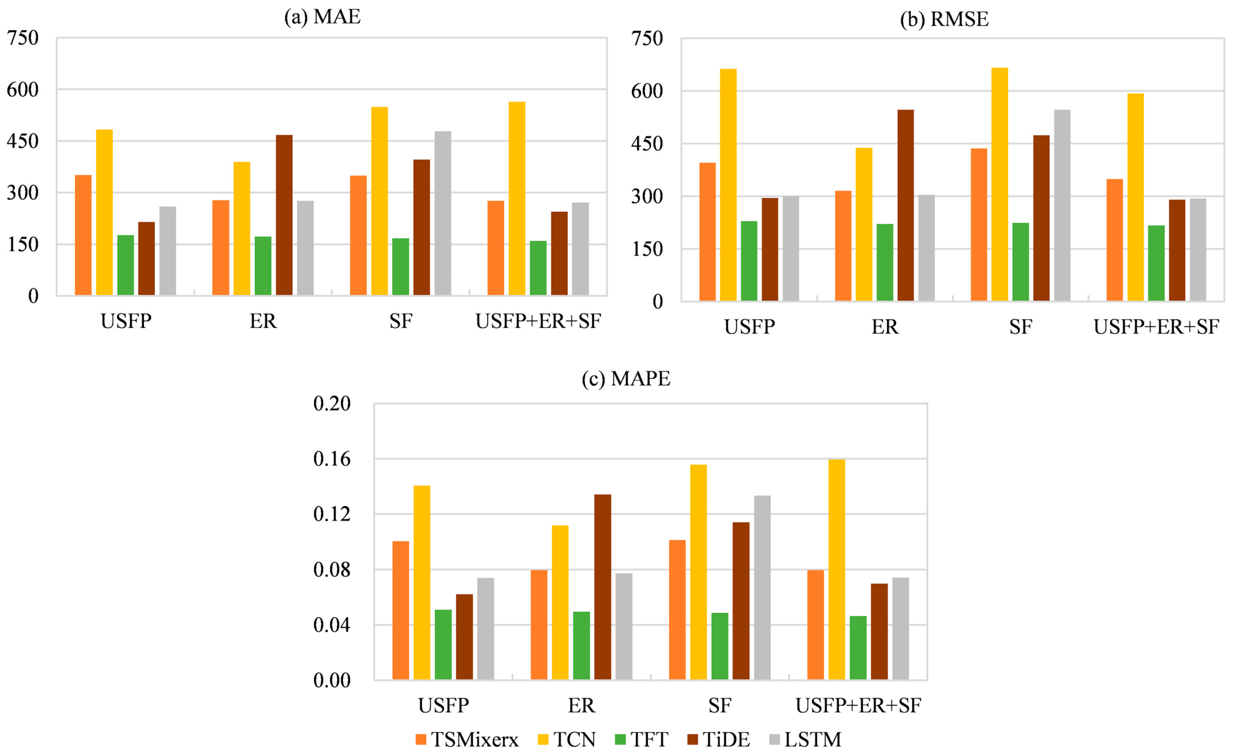
To ensure a fair and reproducible comparison, the multivariate analysis was limited to those model implementations with inherent support for exogenous variables (namely, TSMixerx, TCN, TFT, TiDE, and LSTM). As shown in Figure 2, TFT demonstrates the best overall performance after the incorporation of the exogenous variables USFP, ER, and SF. Specifically, with all three variables included, TFT’s MAE, MAPE, and RMSE are reduced by 41.0%, 37.6%, and 26.2%, respectively, compared to the multivariate LSTM benchmark. TiDE ranks second, showing only a marginal improvement over LSTM.
A detailed comparison of each model’s performance before and after the inclusion of exogenous variables is presented in Table 5. The results reveal that (1) TFT exhibits significant performance improvements under any single-variable setting as well as the full three-variable combination; (2) TiDE demonstrates clear gains from USFP and the three-variable combination, but its performance exhibits instability when ER or SF are added individually; (3) TSMixer derives the most benefit from ER, with only marginal gains from USFP and SF; and (4) both TNC and LSTM exhibit performance degradation after the introduction of any exogenous variables, with SF causing the most pronounced deterioration. This issue primarily stems from architectural limitations: TCN and LSTM lack explicit mechanisms for variable selection, gating, or attention, which hinders their ability to automatically learn and align the complex lagged relationships between exogenous variables and the target series. When exposed to noisy or temporally misaligned external features (e.g., SF), these models fail to filter out irrelevant signals effectively, leading to noise amplification during the prediction process and a consequent degradation in performance.
Analyzing the marginal contributions of the exogenous variables reveals distinct patterns (Table 5). USFP exhibits strong comovement with the target series; however, translating this signal into predictive gains requires models with variable-selection and lag-alignment capabilities. In this regard, TFT and TiDE show the clearest improvements: TFT demonstrates a reduction exceeding 50% across all three error metrics, while TiDE achieves reductions of 35–45%. ER is an information-dense variable whose cadence aligns closely with price fluctuations. TFT demonstrates a remarkable ability to leverage the ER signal, achieving the largest reduction in RMSE (60.5%) among all models. Similarly, TSMixer also benefits from the incorporation of the ER variable, with decreases of 19% to 25% across all metrics. By contrast, SF shows the highest noise level among all exogenous variables, as indicated by its large Coefficient of Variation in Table 3. It also exhibits noticeable lag mismatches, as illustrated in Appendix A.2. Given these characteristics, models that lack sufficient representational capacity or explicit variable-selection mechanisms are more likely to experience performance degradation when SF is included. Only TFT registers a significant gain, whereas the performance of TSMixer, TiDE, TCN, and LSTM deteriorates, with that of TCN degrading the most.
In summary, while exogenous variables can be beneficial for forecasting, their efficacy is highly contingent on model architecture. Specifically, only models equipped with robust variable-selection mechanisms and lag-alignment capabilities are capable of reliably translating these external signals into reproducible performance gains.

3.3. Results: Multi-Horizon Performance Comparison

For the model whose hyperparameters were optimized on the validation set, a single-origin multi-step forecast was performed on the test window. We reported the cumulative temporal mean of MAE, MAPE, and RMSE over increasing forecast horizons (1-k steps, where k ∈ {5, 10, 30, 60}). Since MAE, MAPE, and RMSE exhibit nearly identical trends across varying forecast horizons, we hereafter present the detailed analysis using MAPE as a representative metric.
Without exogenous variables, iTransformer attains the lowest MAPE in the short term (recording 0.0073 and 0.0112 for 5-day and 10-day horizons, respectively), followed closely by TFT, TCN and PatchTST. It also demonstrates a clear advantage over the baseline LSTM (0.0741 and 0.0698 for the same short-term horizons). At the mid-horizon (30 days), TCN becomes slightly best (0.0172), with PatchTST (0.0183) and iTransformer (0.0188) very close. At the long horizon (60 days), iTransformer regains the lead (0.0387), followed by SOFTS and TimesNet, while TFT/TiDE/TSMixerx degrade more visibly with horizon length. Consistent with expectations, prediction errors generally increase with the forecast horizon. However, iTransformer demonstrates robust performance across all horizons, while TCN exhibits greater stability at medium-term horizons (see Figure 3).
When all exogenous variables (USFP, ER, and SF) are incorporated simultaneously, TFT achieves the lowest MAPE across all forecast horizons (5, 10, 30, and 60 days: 0.0061, 0.0106, 0.0150, and 0.0464, respectively), significantly outperforming benchmark LSTM model as well as other deep learning architectures such as TCN, TSMixerx, and TiDE. With single exogenous variables, TFT remains best across all horizons for ER and SF. When augmented solely with USFP, TFT exhibits a slightly higher MAPE (0.0510) compared to the LSTM baseline (0.0440) specifically at the 60-day horizon, while maintaining strong predictive performance at shorter horizons. These results indicate that the gains from exogenous variables depend on both the forecast horizon and the type of covariate (see Figure 4).
To further characterize the interaction between exogenous inputs and forecast horizons, we focus on TFT, whose architecture natively supports covariates and exhibits strong multivariate performance, and quantify its gains under the same evaluation protocol as the univariate (CSFP) baseline. Relative to its univariate baseline, TFT exhibits a systematic reduction in MAPE as the forecast horizon extends in the ALL (USFP + ER + SF) exogenous variables scenario, achieving reductions of 35.5%, 38.2%, 22.2%, and 59.9% at 5, 10, 30, and 60 days, respectively. With single sources, USFP may provide negligible or even slightly negative benefits at very short horizons, whereas ER, SF, and the full variable set (ALL) consistently lead to lower MAPE and more stable performance across horizons (see Figure 5).

4. Discussion

4.1. Model Performance Discussion

The study found that in the univariate prediction setting, iTransformer performs better on MAE and MAPE, whereas TimesNet achieves the best RMSE. iTransformer embeds the entire univariate history as a single “token” and employs a shared feed-forward network (FFN) for strong sequence encoding, effectively capturing intrinsic attributes such as amplitude, periodicity, and trend. This architectural choice underpins its performance advantage on univariate tasks [55]. Souto’s et al. [59] analysis of stock realized-volatility forecasting corroborates TimesNet’s strength in mitigating the impact of extreme market movements, resulting in a substantially lower RMSE. Therefore, TimesNet is more suitable for long-horizon forecasting and for scenarios that demand higher consistency and robustnesss [25,59]. The statistical significance of these performance differences has been confirmed by Wilcoxon signed-rank tests (Appendix C.1). After incorporating exogenous variables, TFT achieved superior overall performance, which is attributable to its built-in variable selection networks and interpretable attention mechanisms [26]. Likewise, Sakib et al. [60] demonstrates that TFT achieves superior accuracy and robustness in solar irradiance forecasting when integrated with multiple meteorological exogenous variables.
This study employs a rigorous out-of-sample evaluation protocol: after temporal data segmentation, a standardizer is fitted exclusively on the training set to prevent data leakage; automated hyperparameter optimization is performed on the validation set; and a one-time “blind test” is ultimately conducted on the test set. All performance metrics are calculated on the inverse-normalized original price scale to ensure the evaluation results directly reflect actual price prediction errors. This single-origin forecasting framework guarantees that test set data remains entirely unused during the training process, significantly enhancing the reliability of the evaluation outcomes. By utilizing cumulative average errors (e.g., MAE, MAPE, RMSE) over the prediction horizon rather than single-step errors for model performance measurement, this study places greater emphasis on the model’s overall stability throughout the entire forecast interval rather than on short-term precision. This methodological approach differs from the evaluation frameworks (e.g., single-step prediction or dynamic rolling prediction) employed in some studies [9,11,37] for soybean futures price prediction models, leading to a “conservative” appearance in direct performance comparisons. Additionally, factors such as the quotation unit, sample period range, dataset scale, forecast horizon setting, selection of futures contract types, and market conditions during the sample period can all influence the model’s final predictive performance. This study is among the first to systematically integrate and apply a range of new-generation deep learning models for forecasting the price of soybean No. 2 futures contract in China, incorporating external market information (e.g., USFP, ER, SF) to construct a comparative analysis framework. The research conclusions demonstrate robustness across multiple relative error metrics, providing an empirical foundation and decision-making reference for subsequent model selection and covariate configuration strategies.
Furthermore, the continuity of futures price series can be compromised by artificial jumps at contract rollovers when splicing data based on maximum open interest. To ensure that our model comparisons are not biased by these potential artifacts, we conducted a focused robustness check by forecasting 5-day log-returns. The results demonstrated a high consistency in model rankings between the return series and the original price series (see Appendix C.2). Top-performing models (e.g., iTransformer, TFT, TCN, PatchTST, TimesNet, SOFTS) remained at the forefront, while weaker models (e.g., TSMixerx, LSTM, TimeLLM) consistently lagged. This stability, confirmed even under the sensitive test of short-term return forecasting, strongly indicates that the relative performance of the models reflects their genuine capacity to capture underlying market dynamics, rather than an overfitting to rollover-induced noise.

4.2. Exogenous Covariates Discussion

While this study incorporates several exogenous variables (e.g., USFP, ER, SF) based on economic relevance and prior literature, it is also important to recognize that not all exogenous information improves model performance. Noman et al. [61] finds that irrelevant exogenous variables harm performance in energy-sector wind-speed forecasting. López-Andreu et al. [62] found that adding multiple sets of exogenous variables to several neural models (e.g., Time2Vec-Transformer, BiLSTM, MDN-BiLSTM) often led to significant performance deterioration or minimal gains. Only a few architectures remained relatively stable when the added variables were highly correlated with the target. This suggests that irrelevant or noisy features can impair a network’s generalization capability. In this study, we observe that USFP and ER typically deliver significant gains (e.g., for TFT, TiDE, and TSMixer), consistent with the literature on the co-movement between U.S. and Chinese soybean prices and on exchange-rate effects on agricultural prices and imports [46,48,63]. Conversely, SF often exhibits significant time lags and is highly susceptible to policy changes and supply–demand dynamics. Models lacking inherent variable selection mechanisms and robust temporal alignment capabilities are particularly susceptible to performance degradation when such features are incorporated. Related research also reports asymmetric and time-varying causality and lead–lag relations between freight rates and commodity prices, indicating that the direction and timing of influence can differ across markets and periods [64].
Overall, this study focuses on predictive accuracy rather than structural causality. The relationships captured by the deep learning models represent data-driven statistical dependencies and dynamic associations among market variables, rather than explicitly modeled causal mechanisms. In addition, the inclusion of the exchange rate variable reflects unhedged market conditions, where currency fluctuations are directly embedded in observed prices. Consequently, the proposed predictive framework is most applicable to market scenarios in which exchange rate risks are not explicitly neutralized through hedging strategies.

4.3. Model Applications Discussion

This study covers nine models with distinct architectures and capabilities. Based on the experimental results and computational costs, we propose the following recommendations: (1) For high-frequency, low-latency univariate forecasting, we recommend iTransformer or SOFTS; to manage extreme volatility and control tail risk, TimesNet is more suitable. (2) For multivariate long-sequence forecasting that requires a balance of low computational cost and solid accuracy, pure-MLP architectures such as TiDE, and TSMixerx are highly effective options; when highly informative exogenous covariates (e.g., USFP, ER) are available and medium- to long-horizon forecasts are needed, TFT is a superior choice with its strong overall performance and built-in uncertainty quantification capabilities. (3) TCN can serve as a computationally efficient baseline model for rapid validation. Furthermore, under the present evaluation framework, Time-LLM and PatchTST failed to outperform baseline or alternative models significantly. Thus, they are not currently recommended as primary choices, though their potential in other contexts remains unexplored.
In addition, the proposed forecasting framework provides quantitatively grounded insights for market operations and policy formulation. Specifically, the best-performing model (TFT) that integrates exogenous variables (USFP, ER, and SF) achieves a 5-day MAPE of 0.6% and maintains a 10-day MAPE of 1.06%. Given the average training-set price of CNY 3945 per ton, these levels of accuracy correspond to average absolute deviations ranging from approximately CNY 24 to 42 per ton, indicating that the model can capture short-term price dynamics with high stability. Such predictive precision offers a solid basis for forward-looking applications in risk monitoring and inventory planning in China’s soybean market. The identified lead–lag relationships between domestic and external factors offer valuable guidance for optimizing hedging strategies, for instance by leveraging the one-week leading effect of SF or the synchronous movement of USFP to dynamically adjust hedge ratios and timing. Moreover, the sensitivity of CSFP to external cost factors reveals the transmission channels of global price shocks to domestic markets, providing policy insights into margin regulation, import timing, and supply-chain stabilization. Overall, the results highlight the framework’s potential to support data-driven decision-making and enhance the robustness of risk management in China’s soybean futures market.

4.4. Limitations and Future Work

Inevitably, this study has several limitations. Although the robustness check using log-return forecasting in this study confirmed that contract rollover gaps did not affect the core conclusions of our model comparison, it should be noted that the continuous series constructed by directly splicing dominant contracts based on open interest has inherent methodological limitations in terms of continuity. Future research could further adopt professional methods such as back-adjusted or ratio-adjusted techniques to construct continuous contracts, thereby more precisely isolating and quantifying the impact of the rollover effect itself on forecasting performance. Secondly, differences in implementation maturity among deep-learning frameworks resulted in only models with stable multivariate and exogenous-covariate support (TFT, TCN, TiDE, TSMixerx and LSTM) being included in the multivariate experiments. Although other advanced architectures such as SOFTS, TimesNet, iTransformer, PatchTST, and Time-LLM are theoretically capable of handling multivariate inputs, their publicly available implementations are primarily tailored for benchmark tasks and currently lack a unified and stable interface for the single-target with exogenous covariates design adopted in this study. This methodological boundary may limit the comprehensiveness of cross-model benchmarking but ensures experimental consistency and reproducibility. Furthermore, this study has not explicitly incorporated such event-type information (e.g., trade friction, pandemics, policy adjustments) into the exogenous variables. The limited coverage of external covariates may lead to distributional shifts during state transition phases, consequently compromising model generalization and robustness.
To address the above limitations, future research should be focused on two main directions. On the data-processing side, future studies adopt back-adjusted and ratio-adjusted continuous series with rolling weights, and include features such as days to expiry, near–far month spreads, and roll yield, accompanied by sensitivity analyses. On the modeling side, future research could extend single-target, multi-covariate comparisons to include iTransformer and related models, and add proxy variables for tariff changes, pandemics and policy uncertainty. In addition, hybrid feature-learning architectures and attention-based fusion mechanisms may be explored to enhance the integration of multiple exogenous variables, improve interpretability through dynamic feature weighting, and strengthen forecasting robustness. Furthermore, the paper’s main results are based on a single-origin evaluation and are reported as cumulative averages over intervals, which stably reflect the overall level across different forecast horizons; these analyses could be supplemented later with a rolling-origin approach to align with mainstream benchmarks.

5. Conclusions

This study is among the first to systematically apply a range of deep learning neural network models to forecast the DCE No. 2 soybean futures price, evaluating their performance while integrating external market information. The findings indicate that in univariate forecasting, iTransformer achieved the lowest MAPE over short (5–10 days) and long (60 days) horizons, while TCN demonstrated the most stable performance at the medium-term horizon (30 days); TimesNet attained the best RMSE, making it more suitable for handling extreme volatility and controlling tail errors. Under multivariate settings (with the introduction of USFP, ER, and SF as exogenous variables), TFT demonstrates the best overall performance, significantly outperforming the LSTM baseline model across nearly all forecast horizons. However, the gains from exogenous variables depend on both the forecast horizon and the choice of covariates. This study provides practitioners with actionable guidance for model selection and covariate configuration and points the way toward future improvements in broader covariate coverage, futures contract data processing, and model evaluation methods.

Author Contributions

Conceptualization, X.D. and L.C.; methodology, Y.H. and Y.C.; software, Y.H.; validation, W.Z. and M.W.; formal analysis, X.D., L.C. and Y.H.; data curation, X.N.; writing—original draft preparation, X.D. and L.C.; writing—review and editing, L.C. and J.L.; supervision, L.C. All authors have read and agreed to the published version of the manuscript.

Funding

This research was funded by the Science and Technology Innovation Project of the Agricultural Information Institute of Chinese Academy of Agricultural Sciences (CAAS-ASTIP-2025-AII) and The Major Science and Technology Mission of the Chinese Academy of Agricultural Sciences (CAAS-ZDRW202509).

Institutional Review Board Statement

Not applicable.

Data Availability Statement

The data presented in this study are available on request from the corresponding author.

Conflicts of Interest

The authors declare no conflicts of interest.

Appendix A

Appendix A.1. Cross-Correlation and Lead–Lag Analysis: Weekly Data
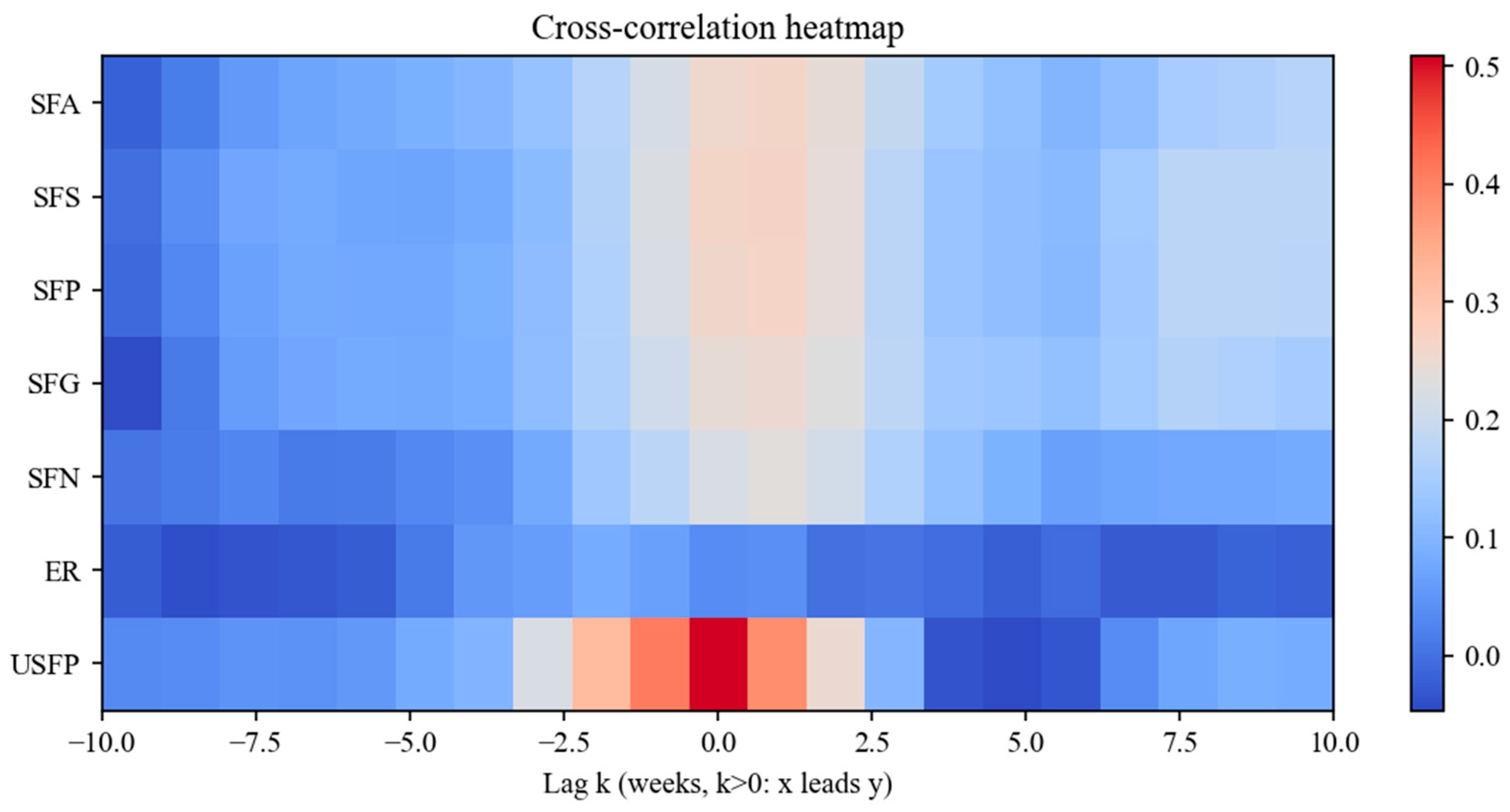
To validate the temporal alignment and causal relevance of the exogenous predictors, cross-correlation functions (CCF) and lag plots were employed to examine the lead–lag structure between CSFP and the external variables USFP, ER, and SF. The analysis was conducted using weekly data smoothed with a 4-week moving average window, with all variables transformed into stationary form (log-returns or first differences).
Figure A1 presents the cross-correlation heatmap across lags ±10 weeks. USFP shows the strongest contemporaneous association with CSFP (best lag k = 0, r ≈ 0.50), whereas SF exhibit clear one-week lead effects (best lag k = 1, r ≈ 0.23–0.27). ER displays a weak but directionally consistent correlation (r ≈ 0.05, k = 1), suggesting limited yet plausible cost-transmission dynamics.
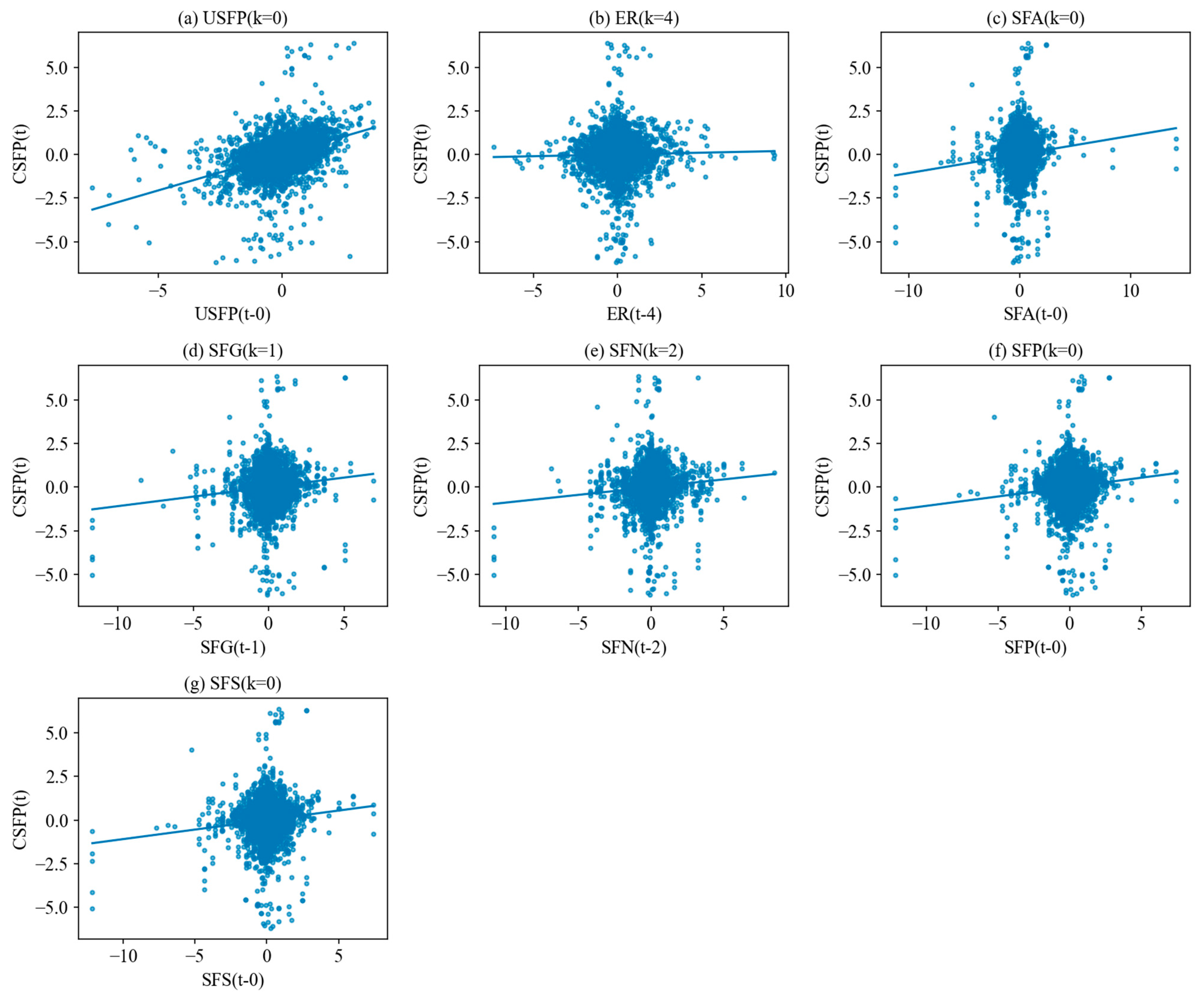
To further illustrate these relationships, lag plots were drawn for each exogenous variable at its best-performing lag (k) identified from the CCF matrix (Figure A2). These plots visualize the contemporaneous and leading relationships: USFP is nearly synchronous with CSFP; SF indices lead by approximately one week; and ER exerts only a mild, noisy influence. Together, the CCF and lag plots confirm that these external variables possess stable temporal structures consistent with their economic interpretations and can be treated as exogenous predictors in the modeling framework.
It is noted that the CCF for ER exhibits mild asymmetry, with a slightly stronger correlation observed when ER follows CSFP by several weeks. However, since the study focuses on predictive relationships, only the non-negative lags (where exogenous variables lead CSFP) were retained for analysis.
Figure A1. Weekly cross-correlation heatmap (smooth_window = 4). The figure illustrates the cross-correlation coefficients (r) between CSFP and three exogenous variables (USFP, ER, and SF) across lags of ±10 weeks. Positive lags indicate that the exogenous variable leads CSFP.
Agriculture 15 02586 g0a1
Figure A2. Weekly lag plots at best lags for exogenous variables: (a) USFP, (b) ER, (c) SFA, (d) SFG, (e) SFN, (f) SFP and (g) SFS.
Agriculture 15 02586 g0a2

Appendix A.2. Cross-Correlation and Lead–Lag Analysis: Daily Data (Robustness Check)
To validate the robustness of the weekly results, an additional cross-correlation analysis was conducted using daily data smoothed with a five-day moving average window. All variables were transformed into stationary series (log-returns or first differences), as confirmed by the ADF tests (p < 0.01 for all series).
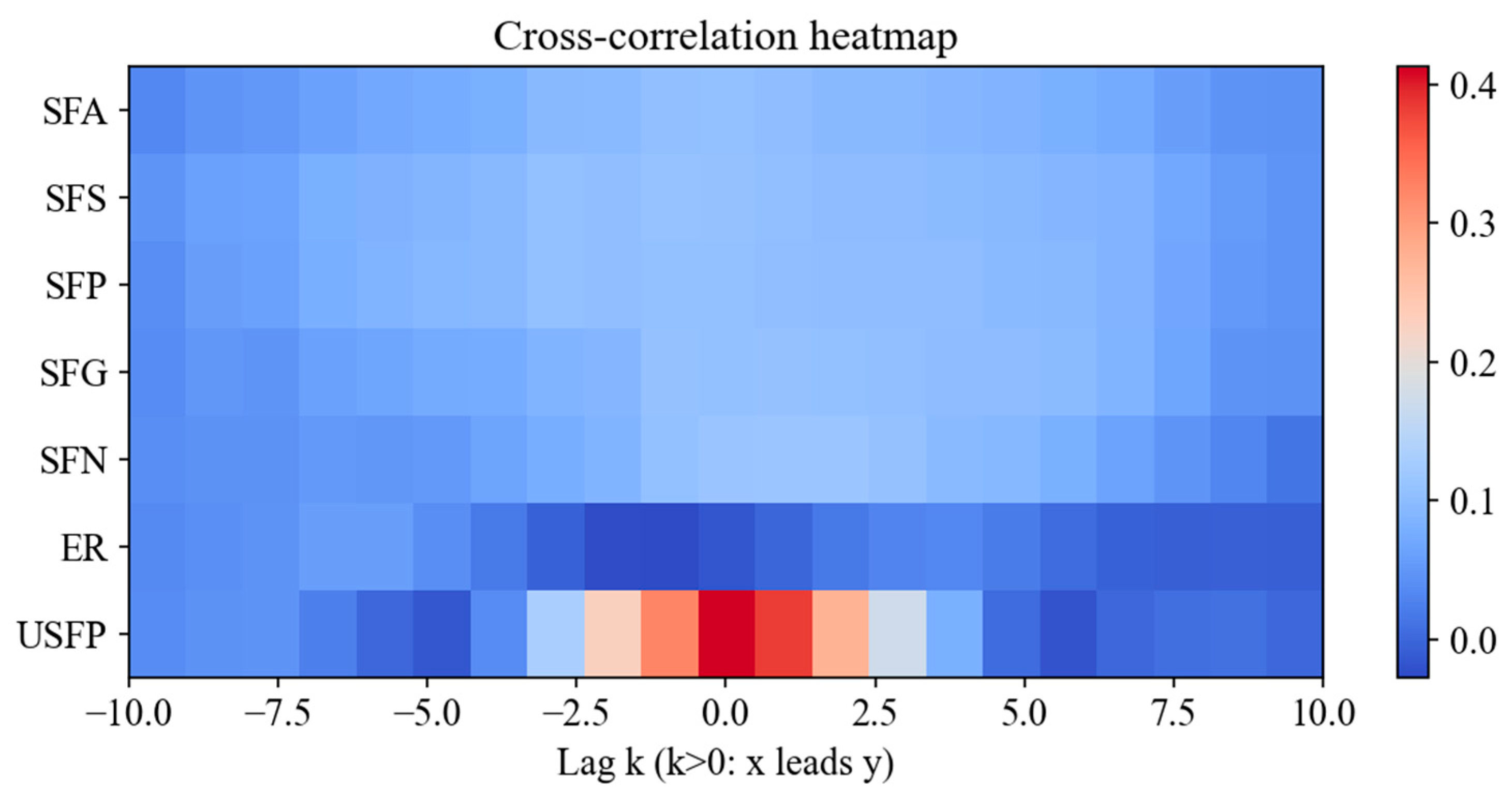
As shown in the daily analysis, USFP remains the most strongly correlated and contemporaneous variable with CSFP (best lag k = 0, r ≈ 0.40). SF also display significant short-term relationships, with moderate correlations (r ≈ 0.10–0.11) and leading effects of approximately two trading days (k = 2 for SFN and SFG). ER exhibits a weaker but still statistically significant correlation (r ≈ 0.03, k = 4), consistent with limited yet plausible cost-transmission dynamics.
Overall, the daily frequency results confirm the robustness of the lead–lag structures identified in the weekly data. The consistency across time resolutions supports the interpretation that USFP and SF serve as economically meaningful exogenous predictors, while ER plays a secondary but directionally coherent role.
Similarly, ER’s full CCF pattern is slightly asymmetric, showing a marginally stronger negative-lag correlation where ER lags behind CSFP. Given the forecasting-oriented scope of this work, only leading (non-negative) lags were considered in the reported analysis.
Figure A3. Daily cross-correlation heatmap (smooth_window = 5). The figure illustrates the cross-correlation coefficients (r) between CSFP and exogenous variables (USFP, ER, and SF) across lags of ±10 trading days. Positive lags indicate that the exogenous variable leads CSFP.
Agriculture 15 02586 g0a3
Figure A4. Daily lag plots at best lags for exogenous variables: (a) USFP, (b) ER, (c) SFA, (d) SFG, (e) SFN, (f) SFP and (g) SFS.
Agriculture 15 02586 g0a4

Appendix B

Appendix B.1. Temporal Dynamics of Major Variables
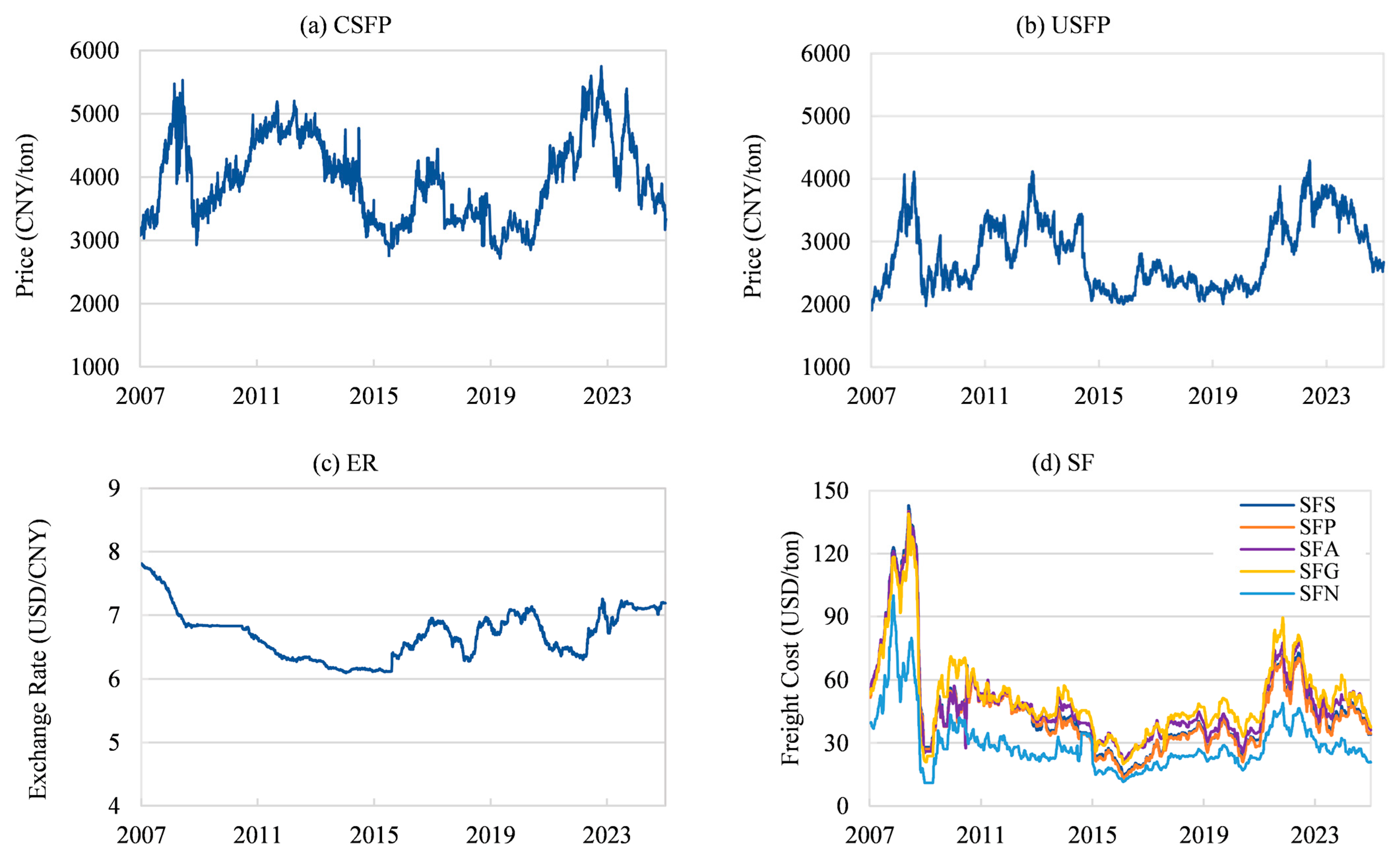
Figure A5. Temporal evolution of (a) the DCE No. 2 soybean futures price (CSFP), (b) U.S. soybean futures price (USFP), (c) the USD/CNY exchange rate (ER), and (d) the soybean freight cost (SF).
Agriculture 15 02586 g0a5

Appendix B.2. Hyperparameter Search Spaces and Model Configurations

Systematic hyperparameter optimization was performed for all trainable models in this study to ensure reliable and comparable results. Importantly, the primary goal of this study is to perform a fair model comparison under a unified experimental protocol, rather than pushing each individual model to its absolute performance limit through exhaustive, architecture-specific tuning.
To this end, we adopted a general-parameter-centric optimization strategy: all models shared an identical search space for general hyperparameters, which included learning rate, batch size, input window length, maximum training steps, and random seed. In addition, for each model, one to three of the most influential architecture-specific parameters were selected and included in the search space, as summarized in Table A1.
Notably, Time-LLM was excluded from hyperparameter tuning. This method relies on a frozen large language model, where structural parameters (such as d_model and n_heads) are fixed by the underlying LLM, and performance primarily depends on prompt design rather than conventional hyperparameter adjustment. Consistent with common practice in foundational LLM-based time series forecasting studies, where the core LLM parameters remain frozen, we evaluated the model using its default configuration.
Table A1. Model Configurations and Hyperparameter Search Space.
CategoryParameterSetting/Search Space
Generallearning_rate10−5–10−2 (log-uniform)
batch_size{8, 16, 32}
input_size{365, 730}
max_steps1000
random_seed1–10
iTransformerd_model64
n_heads4
TiDEhidden_size256
decoder_output_dim{8, 16, 32}
num_encoder_layers/num_decoder_layers{1, 2, 3}
PatchTSTpatch_len{16, 24}
n_heads{4, 16}
TCNn_layers4
kernel_size3
dilationFixed as {1, 2, 4, 8}
TFThidden_size64
n_heads4
SOFTS/TimesNet/TSMixermodel_dim{64, 128}
LSTMhidden_size
n_layers
200
{1, 2, 3}

Appendix C

Appendix C.1. Comprehensive Wilcoxon Signed-Rank Test Analysis
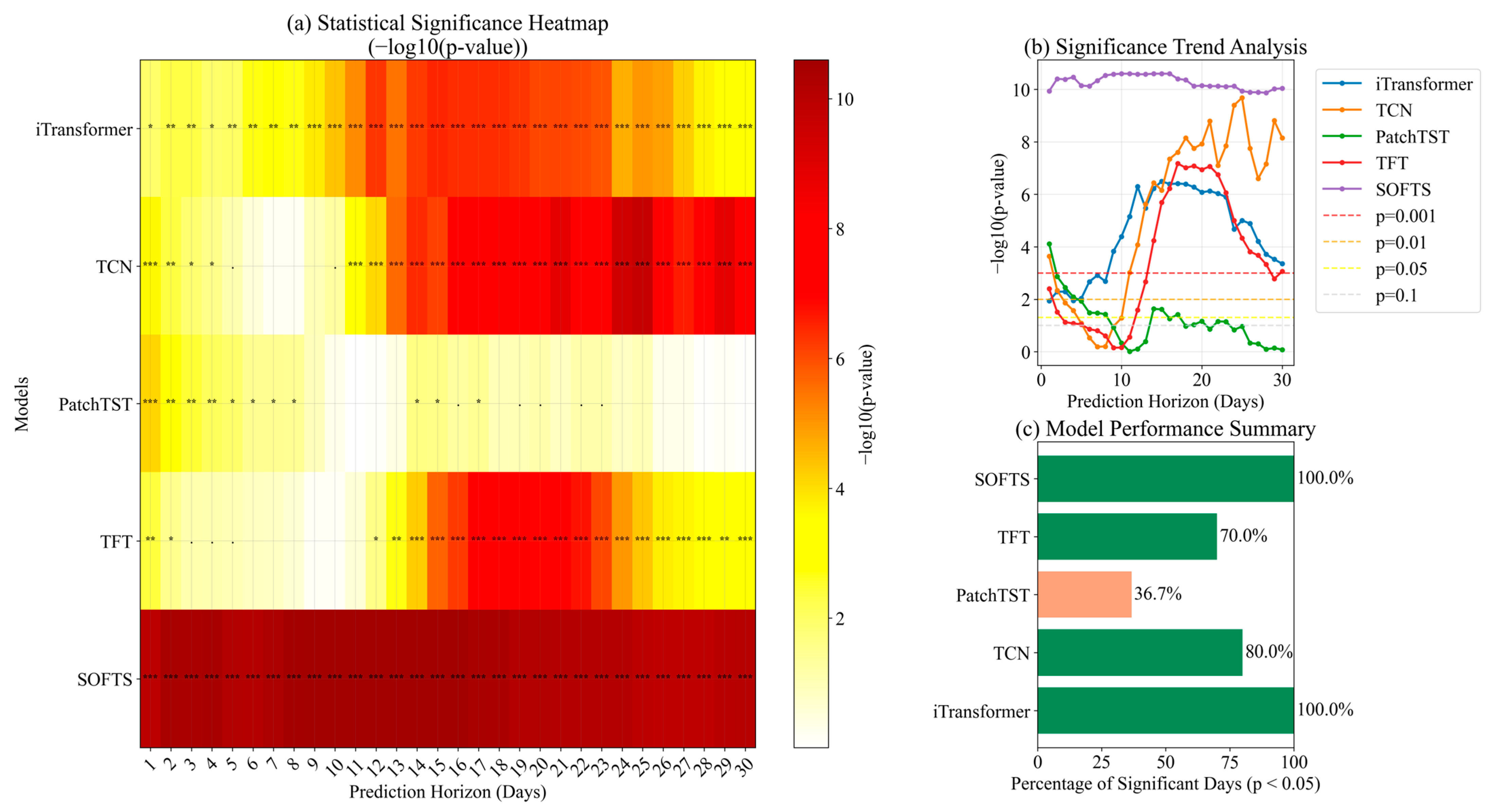
To statistically validate the performance differences among models, we conducted Wilcoxon signed-rank tests using LSTM as the baseline model. Given the multiple forecast horizons and model configurations, the tests were performed for each of the 30 daily prediction horizons to assess the consistency and robustness of statistical significance across time.
The results reveal that SOFTS and iTransformer exhibit consistent and statistically significant superiority over LSTM across all horizons, while TCN and TFT show significance in 80.0% and 70.0% of the prediction days, respectively, and PatchTST shows moderate significance (36.7%). These findings confirm that performance differences among models are statistically meaningful rather than random fluctuations.
Figure A6. Comprehensive Wilcoxon test analysis (Baseline: LSTM) (a) Statistical significance heatmap (–log10(p-value)). Darker shades indicate higher significance, and asterisks (·,*, **, ***) denote significance levels where p < 0.1, 0.05, 0.01, and 0.001, respectively. (b) Significance trend analysis. The evolution of –log10(p-value) across the 30-day prediction horizon, with dashed lines marking standard p-value thresholds. (c) Model performance summary. The percentage of days showing statistically significant improvement (p < 0.05) relative to LSTM for each model.
Agriculture 15 02586 g0a6

Appendix C.2. Robustness Check: Eliminating the Impact of Rollover Jumps

To eliminate the potential impact of artificial price jumps caused by the main contract splicing method during rollover periods on the model prediction results, this study retrained and evaluated all ten models based on log-returns. The log-return series inherently eliminates price-level discontinuities resulting from contract rollovers.
The performance rankings based on MAE and RMSE demonstrate that the relative performance of the models remains largely stable: models such as iTransformer, TFT, TCN, PatchTST, and SOFTS continue to rank at the top, while TSMixerx, LSTM, and TimeLLM remain in the lower tiers. Crucially, no anomalous rank reversals were observed where a model jumped from the bottom to the top tier, or vice versa.
Therefore, it can be confirmed that the findings of this study are not unduly influenced by the price jumps associated with main contract splicing and demonstrate strong robustness.
Table A2. Model ranking comparison: price-level forecasting vs. log-return forecasting.
ModelPrice MAPE (Rank)Return MAE (Rank)Return RMSE (Rank)
iTransformer0.0073 (1)0.002295 (5)0.002547 (5)
TFT0.0094 (2)0.001921 (2)0.002245 (2)
TCN0.01 (3)0.002288 (4)0.002423 (3)
PatchTST0.01 (4)0.002558 (6)0.002771 (6)
TiDE0.0229 (5)0.00684 (10)0.008479 (10)
SOFTS0.0248 (6)0.002187 (3)0.002537 (4)
TimesNet0.028 (7)0.001704 (1)0.001991 (1)
TSMixerx0.0435 (8)0.002952 (8)0.003262 (8)
LSTM0.0741 (9)0.006099 (9)0.007707 (9)
TimeLLM0.0875 (10)0.002806 (7)0.002877 (7)

References

  1. Li, J.L.; Chen, M.; Cui, L. Research on the influence of domestic and foreign soybean futures price on spot price: From the perspective of price linkage. J. Northwest Univ. (Philos. Soc. Sci. Ed.) 2021, 51, 34–42. [Google Scholar] [CrossRef]
  2. Lin, D.Y.; Jin, P.L.; Wang, W.T.; Mao, Y.X. Research on import risks and optimization of import source distribution of soybeans in China. China Oils Fats 2025. Epub ahead of print. [Google Scholar]
  3. General Administration of Customs of the People’s Republic of China. Online Query Platform for Customs Statistics. 2025. Available online: http://stats.customs.gov.cn/ (accessed on 15 August 2025).
  4. National Bureau of Statistics of the People’s Republic of China. Statistical Communiqué of the People’s Republic of China on the 2024 National Economic and Social Development. 2025. Available online: https://www.stats.gov.cn/sj/zxfb/202502/t20250228_1958817.html (accessed on 15 August 2025).
  5. Xiang, C.L. Study on the Influencing Factors and Forecast of Soybean Prices in China. Ph.D. Thesis, Anhui University of Agriculture, Hefei, China, 2024. [Google Scholar]
  6. Hu, X.R.; Zhang, Y.M.; Fan, S.G.; Chen, K.Z.; Wu, Q. The impact of extreme weather events on global soybean markets and China’s imports. J. Agric. Econ. 2025, 76, 251–267. [Google Scholar] [CrossRef]
  7. Wang, X.N.; Yi, L. Optimization of grain import market layout in the context of food security: A study of soybean in China. Front. Sustain. Food Syst. 2025, 9, 1549463. [Google Scholar] [CrossRef]
  8. Jiang, X.Y.; Li, H.S.; Dai, X.; Li, J.D.; Liu, Y. An empirical analysis of global soybean supply potential and China’s diversified import strategies based on global agro-ecological zones and multi-objective nonlinear programming models. Agriculture 2025, 15, 529. [Google Scholar] [CrossRef]
  9. Xu, Y.L.; Kang, M.Z.; Wang, X.J.; Hua, J.; Wang, H.Y.; Shen, X. Corn and soybean futures price intelligent forecasting based on deep learning. Smart Agric. 2022, 4, 156–163. [Google Scholar] [CrossRef]
  10. Xu, Y.Y.; Pan, F.H.; Wang, C.M.; Li, J. Dynamic price discovery process of Chinese agricultural futures markets: An empirical study based on the rolling window approach. J. Agric. Appl. Econ. 2019, 51, 664–681. [Google Scholar] [CrossRef]
  11. Luo, Y.L. Soybean futures price prediction based on CNN-LSTM model of Bayesian optimization algorithm. Highlights Business Econ. Manag. 2023, 16, 6–17. [Google Scholar] [CrossRef]
  12. Czudaj, R.L. The role of uncertainty on agricultural futures markets: Momentum trading and volatility. Stud. Nonlinear Dyn. Econom. 2020, 24, 20180054. [Google Scholar] [CrossRef]
  13. Xiong, T.; Bao, Y.K. Research on soybean futures price prediction based on dynamic model average. China Manag. Sci. 2020, 28, 79–88. [Google Scholar] [CrossRef]
  14. Li, M.; Xiong, T. Do bubbles alter contributions to price discovery? Evidence from the Chinese soybean futures and spot markets. Emerg. Mark. Financ. Trade 2019, 55, 3417–3432. [Google Scholar] [CrossRef]
  15. Zhang, T.T.; Tang, Z.P. Agricultural commodity futures prices prediction based on a new hybrid forecasting model combining quadratic decomposition technology and LSTM model. Front. Sustain. Food Syst. 2024, 8, 1334098. [Google Scholar] [CrossRef]
  16. Zhang, J.; Zhen, L.L.; Zhai, D.S. Forecasting for soybean futures based on multistage attention mechanism. Syst. Eng. 2023, 41, 148–158. [Google Scholar]
  17. Yan, H.J. Integrated prediction of financial time series based on deep learning. Stat. Inf. Forum 2020, 35, 33–41. [Google Scholar] [CrossRef]
  18. Hou, Y.; Sun, T.; Cui, Y.P.; Wang, X.D.; Zhao, A.P.; Wang, T.; Wang, Z.F.; Yang, W.J.; Gu, G. Vegetable price prediction based on optimized neural network time series models. Smart Agric. 2025. Epub ahead of print. [Google Scholar]
  19. Manogna, R.L.; Dharmaji, V.; Sarang, S. Enhancing agricultural commodity price forecasting with deep learning. Sci. Rep. 2025, 15, 20903. [Google Scholar] [CrossRef]
  20. Nikou, M.; Mansourfar, G.; Bagherzadeh, J. Stock price prediction using deep learning algorithm and its comparison with machine learning algorithms. Int. J. Intell. Syst. Account. Financ. Manag. 2019, 26, 164–174. [Google Scholar] [CrossRef]
  21. Ji, S.; Kim, J.; Im, H. A comparative study of bitcoin price prediction using deep learning. Mathematics 2019, 7, 898. [Google Scholar] [CrossRef]
  22. Wang, Y.X.; Liu, Q.Y.; Hu, Y.R.; Liu, H.J. A study of futures price forecasting with a focus on the role of different economic markets. Information 2024, 15, 817. [Google Scholar] [CrossRef]
  23. Liu, H.T.; Pan, Y.; Liu, W.; Wang, J.Y. A prediction model for soybean meal futures price based on CNN-ILSTM-SA. IEEE Access 2024, 12, 111663–111672. [Google Scholar] [CrossRef]
  24. Wang, Z.L.; French, N.; James, T.; Schillaci, C.; Chan, F.; Feng, M.; Lipani, A. Climate and environmental data contribute to the prediction of grain commodity prices using deep learning. J. Sustain. Agric. Environ. 2023, 2, 251–265. [Google Scholar] [CrossRef]
  25. Wu, H.X.; Hu, T.G.; Liu, Y.; Zhou, H.; Wang, J.M.; Long, M.S. TimesNet: Temporal 2D-variation modeling for general time series analysis. In Proceedings of the Eleventh International Conference on Learning Representations (ICLR 2023), Kigali, Rwanda, 1–5 May 2023. [Google Scholar] [CrossRef]
  26. Lim, B.; Arık, S.Ö.; Loeff, N.; Pfister, T. Temporal fusion transformers for interpretable multi-horizon time series forecasting. Int. J. Forecast. 2021, 37, 1748–1764. [Google Scholar] [CrossRef]
  27. Xiong, T.; Hu, Z.Y. Soybean futures price forecasting using dynamic model averaging: Do the predictors change over time? Emerg. Mark. Financ. Trade 2019, 57, 1198–1214. [Google Scholar] [CrossRef]
  28. Pang, X.Y. Soybean Futures Price Prediction Based on Multimodal Data and LSTM Modeling. Master’s Thesis, Chongqing University of Technology, Chongqing, China, 2025. [Google Scholar]
  29. Srichaiyan, P.; Tippayawong, K.Y.; Boonprasope, A. Forecasting soybean futures prices with adaptive AI models. IEEE Access 2025, 13, 48239–48256. [Google Scholar] [CrossRef]
  30. Xu, Z.L.; Deng, H.L.; Wu, Q.F. Prediction of soybean price trend via a synthesis method with multistage model. Int. J. Agric. Environ. Inf. Syst. 2021, 12, 13. [Google Scholar] [CrossRef]
  31. Liu, J.D.; Zhang, B.; Zhang, T.H.; Wang, J.Y. Soybean futures price prediction model based on EEMD-NAGU. IEEE Access 2023, 11, 99328–99338. [Google Scholar] [CrossRef]
  32. Wang, C.Y. Forecast on price of agricultural futures in China based on ARIMA model. Asian Agric. Res. 2016, 11, 12–16. [Google Scholar] [CrossRef]
  33. Wang, C.H.; Gao, Q. High and low prices prediction of soybean futures with LSTM neural network. In Proceedings of the IEEE 9th International Conference on Software Engineering and Service Science (ICSESS), Beijing, China, 23–25 November 2018; pp. 140–143. [Google Scholar] [CrossRef]
  34. Fan, J.M.; Liu, H.J.; Hu, Y.R. Soybean future prices forecasting based on LSTM deep learning. Prices Mon. 2021, 2, 7–15. [Google Scholar] [CrossRef]
  35. Yin, T.; Wang, Y.M. Nonlinear analysis and prediction of soybean futures. Agric. Econ. 2021, 67, 200–207. [Google Scholar] [CrossRef]
  36. An, W.Y.; Wang, L.; Zeng, Y.R. Text-based soybean futures price forecasting: A two-stage deep learning approach. J. Forecast. 2023, 42, 312–330. [Google Scholar] [CrossRef]
  37. Chen, D.Y.; Liu, H.; Li, Y.F.; Duan, Z. An improved deep learning model for soybean future price prediction with hybrid data preprocessing strategy. Front. Agric. Sci. Eng. 2025, 12, 208–230. [Google Scholar] [CrossRef]
  38. Wang, N.Y.; Houston, J. An intervention analysis on the relationship between futures prices of non-GM and GM contract soybeans in China. J. Bus. Econ. Policy 2015, 2, 1–29. [Google Scholar] [CrossRef]
  39. Li, C.; Hayes, D.J. Price discovery on the international soybean futures markets: A threshold co-integration approach. J. Futures Mark. 2017, 37, 52–70. [Google Scholar] [CrossRef]
  40. Hao, J.; He, F.; Liu-Chen, B.A.; Li, Z.H. Price discovery and its determinants for the Chinese soybean options and futures markets. Financ. Res. Lett. 2021, 40, 101689. [Google Scholar] [CrossRef]
  41. Bandyopadhyay, A.; Rajib, P. The impact of Sino–US trade war on price discovery of soybean: A double-edged sword? J. Futures Mark. 2023, 43, 858–879. [Google Scholar] [CrossRef]
  42. Wang, X.Y.; Zhou, J.J. Correlation analysis of soybean futures prices between China and the United States: Based on wavelet analysis and Copula model. Prices Mon. 2024, 45, 22–29. [Google Scholar] [CrossRef]
  43. Liu, K.; Mu, Y.Y. Price fluctuation and linkage of soybean futures markets in China and the United States. Chin. Agric. Sci. Bull. 2017, 33, 159–164. [Google Scholar]
  44. He, L.Y.; Wang, R. A tale of two markets: Who can represent the soybean futures markets in China? Afr. J. Bus. Manag. 2011, 5, 826–832. [Google Scholar] [CrossRef]
  45. Li, M.; Xiong, T. Dynamic price discovery in Chinese agricultural futures markets. J. Asian Econ. 2021, 76, 101370. [Google Scholar] [CrossRef]
  46. Xu, X.C.; Cai, S.S.; Zhang, L.Y. Dynamic influence of international price fluctuation on soybean market price in China: Based on Bayesian-VAR model. Front. Sustain. Food Syst. 2025, 9, 1594210. [Google Scholar] [CrossRef]
  47. Wu, B.R.; Yu, S.H.; Lv, S.X. Explainable soybean futures price forecasting based on multi-source feature fusion. J. Forecast. 2025, 44, 1363–1382. [Google Scholar] [CrossRef]
  48. Gao, X.; Insuwan, A.; Li, Z.R.; Tian, S.R. The dynamics of price discovery between the U.S. and Chinese soybean market: A wavelet approach to understanding the effects of Sino-US trade conflict and COVID-19 pandemic. Data Sci. Manag. 2024, 7, 35–46. [Google Scholar] [CrossRef]
  49. Wang, X.Y.; Zhang, L.L.; Cheng, Q.Y.; Shi, S.; Niu, H.W. What drives risk in China’s soybean futures market? Evidence from a flexible GARCH-MIDAS model. J. Appl. Econ. 2022, 25, 454–475. [Google Scholar] [CrossRef]
  50. Han, L.; Chen, X.Y.; Ye, H.J.; Zhan, D.C. SOFTS: Efficient multivariate time series forecasting with series-core fusion. arXiv 2024, arXiv:2404.14197. [Google Scholar] [CrossRef]
  51. Das, A.; Kong, W.H.; Leach, A.; Mathur, S.; Sen, R.; Yu, R. Long-term forecasting with TiDE: Time-series dense encoder. In Proceedings of the Twelfth International Conference on Learning Representations (ICLR 2024), Vienna, Austria, 7–11 May 2024. [Google Scholar] [CrossRef]
  52. Chen, S.A.; Li, C.L.; Yoder, N.C.; Arik, S.; Pfister, T. TSMixer: An All-MLP architecture for time series forecasting. arXiv 2023, arXiv:2303.06053. [Google Scholar] [CrossRef]
  53. Bai, S.J.; Kolter, J.Z.; Koltun, V. An empirical evaluation of generic convolutional and recurrent networks for sequence modeling. arXiv 2018, arXiv:1803.01271. [Google Scholar] [CrossRef]
  54. Nie, Y.Q.; Nguyen, N.H.; Sinthong, P.; Kalagnanam, J. A time series is worth 64 words: Long-term forecasting with transformers. In Proceedings of the Eleventh International Conference on Learning Representations (ICLR 2023), Kigali, Rwanda, 1–5 May 2023. [Google Scholar] [CrossRef]
  55. Liu, Y.; Hu, T.G.; Zhang, H.R.; Wu, H.X.; Wang, S.Y.; Ma, L.T.; Long, M.S. iTransformer: Inverted transformers are effective for time series forecasting. In Proceedings of the Twelfth International Conference on Learning Representations (ICLR 2024), Vienna, Austria, 7–11 May 2024. [Google Scholar] [CrossRef]
  56. Metin, A.; Kasif, A.; Catal, C. Temporal fusion transformer-based prediction in aquaponics. J. Supercomput. 2023, 79, 19934–19958. [Google Scholar] [CrossRef]
  57. Jin, M.; Wang, S.Y.; Ma, L.T.; Chu, Z.X.; Zhang, J.Y.; Shi, X.M.; Chen, P.Y.; Liang, Y.X.; Li, Y.F.; Pan, S.R.; et al. Time-LLM: Time series forecasting by reprogramming large language models. In Proceedings of the Twelfth International Conference on Learning Representations (ICLR 2024), Vienna, Austria, 7–11 May 2024. [Google Scholar] [CrossRef]
  58. Zhang, X.Y.; Chowdhury, R.R.; Gupta, R.K.; Shang, J.B. Large language models for time series: A survey. arXiv 2024. [Google Scholar] [CrossRef]
  59. Souto, H.G. Charting new avenues in financial forecasting with TimesNet: The impact of intraperiod and interperiod variations on realized volatility prediction. Expert Syst. Appl. 2024, 255, 124851. [Google Scholar] [CrossRef]
  60. Sakib, S.; Mahadi, M.K.; Abir, S.R.; Moon, A.M.; Shafiullah, A.; Ali, S.; Faisal, F.; Nishat, M.M. Attention-based models for multivariate time series forecasting: Multi-step solar irradiation prediction. Heliyon 2024, 10, e27795. [Google Scholar] [CrossRef] [PubMed]
  61. Noman, F.; Alkawsi, G.; Alkahtani, A.A.; Al-Shetwi, A.Q.; Tiong, S.K.; Alalwan, N.; Ekanayake, J.; Alzahrani, A.I. Multistep short-term wind speed prediction using nonlinear auto-regressive neural network with exogenous variable selection. Alex. Eng. J. 2021, 60, 1221–1229. [Google Scholar] [CrossRef]
  62. López-Andreu, F.J.; López-Morales, J.A.; Hernández-Guillen, Z.; Carrero-Rodrigo, J.A.; Sánchez-Alcaraz, M.; Atenza-Juárez, J.F.; Erena, M. Deep learning-based time series forecasting models evaluation for the forecast of chlorophyll a and dissolved oxygen in the mar menor. J. Mar. Sci. Eng. 2023, 11, 1473. [Google Scholar] [CrossRef]
  63. Gale, F.; Tuan, F.C. China Currency Appreciation Could Boost U.S. Agricultural Exports; U.S. Department of Agriculture, Economic Research Service: Washington, DC, USA, 2007. Available online: https://ers.usda.gov/publications/pub-details?pubid=40462&utm_source=chatgpt.com (accessed on 15 October 2025).
  64. Bandyopadhyay, A.; Rajib, P. The asymmetric relationship between Baltic Dry Index and commodity spot prices: Evidence from nonparametric causality-in-quantiles test. Miner. Econ. 2023, 36, 217–237. [Google Scholar] [CrossRef]
Figure 1. End-to-end workflow of the soybean futures forecasting pipeline. The TPE algorithm is used for hyperparameter optimization within the training-validation loop. The final model, retrained on the combined training and validation sets with the optimal hyperparameters, is evaluated on the held-out test set.
Agriculture 15 02586 g001
Figure 2. Forecasting performance of five deep learning models for DCE No. 2 soybean futures under different exogenous-variable settings, evaluated using three error metrics: (a) MAE, (b) RMSE, and (c) MAPE. All subfigures compare model performance across four exogenous configurations: USFP, ER, SF, and ALL (USFP + ER + SF).
Agriculture 15 02586 g002
Figure 3. Horizon-wise forecasting performance (MAPE) of deep learning models for DCE No. 2 soybean futures without exogenous variables. Bars present the cumulative MAPE averaged over 1–5, 1–10, 1–30, and 1–60-day prediction windows; lower values indicate better forecasting accuracy.
Agriculture 15 02586 g003
Figure 4. Horizon-wise forecasting performance (MAPE) of deep learning models for DCE No. 2 soybean futures under different exogenous-variable settings. (a) ALL (USFP + ER + SF); (b) USFP; (c) ER; (d) SF. Lines plot the cumulative MAPE averaged over the corresponding prediction windows.
Agriculture 15 02586 g004
Figure 5. MAPE change (%) of the TFT model relative to the univariate baseline across different forecast horizons. Lower values indicate improved forecasting accuracy after introducing exogenous variables. At the 60-day horizon, TFT achieves similar MAPE reductions of 55.9% (USFP), 57.9% (SF), 57.2% (ER), and 59.9% (ALL).
Agriculture 15 02586 g005
Table 1. Literature on soybean futures price prediction.
Futures ProductModels/AlgorithmsExogenous VariableReference
CN Soy FutPM: dynamic model averaging (DMA) and dynamic model selection (DMS) framework
BM: Time-Varying Parameter (TVP); Recursive OLS-AR (3); Recursive OLS-All predictors; Random walk
Chinese soybean futures price; Chinese soybean net import; Chinese soybean spot price; U.S. soybean futures price; Trading Volume in Chinese soybean futures markets; Turnover rate in Chinese soybean futures markets; WTl Crude oil spot price; Exchange rate of USD/CNY; Baltic dry index[27]
CN Soy Fut (#1)PM: BO-CNN-LSTM
BM: BP neural network; LSTM; CNN-LSTM
Opening price (OP); Highest price (HP); Lowest price (LP); Closing price (CP); Trading volume (TV); Transaction amount (TA); Open interest (OT)[11]
CN Soy Fut (#1)PM: LSTM
BM: GRU; RNN
OP; HP; LP; CP; TV; TA; OT; 10-day moving average; Moving average convergence divergence; Bias ratio; Larry Williams’ percent range; Relative strength index; Rate of change; Domestic and international news; et al. [28]
US Soy FutPM: Elastic Net; Support Vector Regression (SVR); Decision Tree; Random Forest; Gradient Boosting; LSTM; ANN; Autoregressive Integrated Moving Average with Exogenous Variables (ARIMAX); Seasonal Autoregressive Integrated Moving Average with exogenous variables (SARIMAX)US dollar index; Gold (XAU/USD); Crude oil (WTI/USD); Fertilizers price index; Freight rates; Shipping rates; Weather report; Soybean planting chart; Agriculture planting chart; Bulk grain prices; Soybean future price; Import rate[29]
CN Soy FutPM: LSTM
BM: RNN; GRU; ANN
N/A[30]
CN Soy Fut (#1)PM: Attention-LSTM
BM: Autoregressive Integrated Moving Average (ARIMA); SVR; LSTM
N/A[9]
CN Soy FutPM: Ensemble Empirical Mode Decomposition (EEMD) and New Attention Gate Unit (NAGU) model (EEMD-NAGU)
BM: SVR; LSTM; GRU; NAGU; EEMD-LSTM; EEMD-GRU; Attention-LSTM; Attention-GRU; EEMD-Attention-LSTM; EEMD-Attention-GRU;
Dow Jones Industrial Index (DJIA); S&P Dow Jones Indices Index (S&P 500); National Association of Securities Dealers Automated Quotations Index (NASDAQ)[31]
CN Soy FutPM: ARIMAN/A[32]
CN Soy FutPM: LSTM
BM: BP
N/A[33]
CN Soy Fut (#1)PM: Multistage Attention Network (MAN)
BM: VAR; LSTM
CP; OP; HP; LP; Price fluctuation; Temperature index; Air pressure index; Precipitation index; Search index[16]
CN Soy Fut IndexPM: Multi-layer LSTM
BM: ARIMA; Multi-Layer Perceptron (MLP); SVR
N/A[34]
US Soy FutPM: chaotic artificial neural network (CANN)
BM: ANN
N/A[35]
CN Soy FutPM: Two-Stage Hybrid-LSTM
BM: univariate LSTM; multivariate LSTM; eXtreme Gradient Boosting
Social media text feature[36]
CN Soy Fut (#1)
US Soy Fut
IT Soy ETF
PM: ICEEMDAN-LZC-BVMD-SSA-DELM (a hybrid model composed of improved complete ensemble empirical mode decomposition with adaptive noise (ICEEMDAN); Lempel-Ziv complexity (LZC) determination method; variational mode decomposition optimized by beluga whale optimization (BWO) algorithm (BVMD); sparrow search algorithm (SSA); deep extreme learning machine (DELM))
BM: ELM; radial basis function (RBF); deep belief network (DBN); LSTM; GRU; DELM; SSA-DELM; ICEEMDAN-DELM; ICEEMDAN-SSA-DELM; VMD-DELM; BVMD-DELM; BVMD-SSA-DELM; ICEEMDAN-LZ-BVMD-DELM
N/A[37]
Note: CN = China; US = United States; IT = Italy; Soy = soybean; Fut = futures; #1 = contract No. 1; N/A = not applicable; PM = proposed model; BM = baseline model.
Table 2. Variable definitions and data sources.
VariableDescriptionSource
Target variablesCSFPChina’s DCE No. 2 soybean futures priceDalian Commodity Exchange Data Center
Exogenous variablesUSFPU.S. CBOT soybean futures priceChina Grain and Oil Business Network Data Center
ERExchange rate of USD/CNYChina Foreign Exchange Trade System
SFSSoybean Freight Cost (Santos, Brazil–North China)China Grain and Oil Business Network Data Center
SFPSoybean Freight Cost (Paranaguá, Brazil–China)China Grain and Oil Business Network Data Center
SFASoybean Freight Cost (Argentina–Northern China)China Grain and Oil Business Network Data Center
SFGSoybean Freight Cost (U.S. Gulf Coast -China)China Grain and Oil Business Network Data Center
SFNSoybean Freight Cost (U.S. Pacific Northwest–China)China Grain and Oil Business Network Data Center
Note: Data are obtained from official and verifiable sources, including the Dalian Commodity Exchange Data Center, the China Foreign Exchange Trade System, and the China Grain and Oil Business Network Data Center (institutional subscription). Public data are freely available from http://www.dce.com.cn/dalianshangpin/xqsj/lssj/index.html (accessed on 11 August 2025) and https://www.chinamoney.com.cn/chinese/bkccpr/ (accessed on 11 August 2025), while subscription-based data are available upon request from https://www.fao.com.cn/DataCenter.html (accessed on 7 August 2025).
Table 3. Descriptive statistics of the dataset.
VariableMeanMaxMinStandard
Deviation
Coefficient of VariationUnit
CSFP3957.005751.002709.00655.290.17CNY/T
USFP2795.264289.141906.37541.600.19CNY/T
ER6.707.816.090.390.06-
SFS45.67143.0013.7022.780.50USD/T
SFP44.39140.0612.2022.400.50USD/T
SFA48.88140.0021.1021.140.43USD/T
SFG51.86139.0020.0020.040.39USD/T
SFN29.41100.0011.0013.370.45USD/T
Note: USFP data were originally denominated in U.S. dollars and converted into Chinese yuan (CNY) using the contemporaneous USD/CNY exchange rate obtained from the China Foreign Exchange Trade System.
Table 4. Performance evaluation of the models (multi-horizon average over 1–90 steps).
FrameworkModels/AlgorithmsMAEMAPERMSE
MLPSOFTS140.99260.0407187.8455
TiDE388.53660.1118459.8178
TSMixerx343.57630.0993419.1471
CNNTCN216.58800.0631291.8825
TimesNet147.38280.0412184.7208
TransformerPatchTST206.57810.0600270.9045
iTransformer133.41710.0387186.6440
TFT395.07300.1157558.9772
LMMTime-LLM438.06080.1260505.6690
RNNLSTM237.90260.0653264.0886
Table 5. Impact of exogenous variables on forecasting performance metrics (MAE, MAPE, RMSE).
External VariablesModelΔMAE (%)ΔMAPE (%)ΔRMSE (%)
USFPTFT+55.4+55.9+59.0
TiDE+44.8+44.4+35.9
TSMixer−2.1−1.0+5.6
TCN−123.2−122.5−127.0
LSTM−8.9−13.5−13.6
ERTFT+56.5+57.2+60.5
TSMixer+19.2+19.7+24.7
TiDE−20.3−20.0−18.7
TCN−79.7−76.9−49.9
LSTM−15.9−18.5−15.3
SFTFT+57.6+57.9+59.9
TSMixer−1.6−1.8−4.0
TiDE−1.9−2.0−3.1
TCN−153.4−146.4−128.3
LSTM−100.9−104.1−107.0
USFP + ER + SFTFT+59.6+59.9+61.3
TiDE+37.0+37.5+36.8
TSMixer+19.6+19.8+16.8
TCN−160.2−152.6−103.0
LSTM−13.9−13.7−11.2
Note: All “Δ” values in the table represent the magnitude of change relative to the univariate version of each respective model; “+” indicates a decrease in the metric (denoting better performance), while “−” indicates an increase in the metric (denoting worse performance).
Disclaimer/Publisher’s Note: The statements, opinions and data contained in all publications are solely those of the individual author(s) and contributor(s) and not of MDPI and/or the editor(s). MDPI and/or the editor(s) disclaim responsibility for any injury to people or property resulting from any ideas, methods, instructions or products referred to in the content.