Article

Probabilistic Deep Learning Framework for Greenhouse Microclimate Prediction with Time-Varying Uncertainty and Covariance Analysis

1
Department of Agricultural Machinery Engineering, Jeonbuk National University, Jeonju 54896, Republic of Korea
2
Department of Bioindustrial Machinery Engineering, Jeonbuk National University, Jeonju 54896, Republic of Korea
3
Institute pf Agricultural Machinery & ICT Convergence, Jeonbuk National University, Jeonju 54896, Republic of Korea
*
Author to whom correspondence should be addressed.
Agriculture 2025, 15(23), 2461; https://doi.org/10.3390/agriculture15232461
Submission received: 28 October 2025 / Revised: 25 November 2025 / Accepted: 25 November 2025 / Published: 27 November 2025

Abstract

Although greenhouse microclimates typically exhibit gradual and near-linear transitions, abrupt fluctuations in external weather conditions and actuator operations introduce nonlinear dynamics that complicate accurate interpretation and prediction. Predicting greenhouse microclimate is a key element for achieving stable and energy efficient crop production, particularly in strawberry greenhouse. However, existing greenhouse microclimate deterministic prediction models do not adequately reflect the nonlinear, time-varying characteristics of greenhouses and the inherent uncertainty in data, limiting probabilistic decision-making. In this study, we developed a probabilistic deep learning framework to estimate and interpret uncertainty while simultaneously predicting greenhouse microclimate quantitatively. The proposed one-dimensional convolutional neural network model learned the time-series characteristics of greenhouse internal and external environmental information and control data, predicting a total of nine parameters, including three-dimensional predicted values 3 h later and six-dimensional covariance elements. The model demonstrated high sharpness and calibration performance, with an average R2 of 0.93, a negative log likelihood of 2.08, and a Coverage 90% of 0.901 for three microclimates. In addition, the estimated covariance matrix was used to interpret the time-varying correlations between microclimate variables, confirming local simultaneous variability not captured by global correlation analysis. These results suggest that the model in this study can provide greenhouse operators with explainable uncertainty interpretation and robust control decision support information.

1. Introduction

The stable production of high-quality and high-yield crops is achieved through the optimization of greenhouse environmental control decisions [1]. Such optimization is based on a foundation of empirically accumulated experience and experimentally validated knowledge, enabling growers to achieve both high productivity and enhanced energy efficiency [2]. Decision-making for environmental control relies on predicting fluctuations within the greenhouse microclimate while simultaneously integrating the effects of external weather conditions and the operation of control devices [3].
Advances in computing resources and deep learning algorithms have enabled multidimensional data analysis techniques to predict greenhouse microclimate [4,5]. To predict time-series changes in greenhouse microclimate for optimal growth conditions, research has focused on using deep learning models to learn from the external environment, the operating status of greenhouse control actuators, and time-series changes in greenhouse microclimate [6,7]. Furthermore, research has been conducted to implement real-time prediction-control loop optimization and incorporate safety constraints by applying learning-based model predictive control techniques that utilize predictions from learned models [8,9]. Previous research has focused on improving energy efficiency and reducing microclimate constraint violations during greenhouse actuator operation by applying state-of-the-art algorithms [10,11]. However, existing control loop implementation studies often utilize deterministic predictive models, which fail to accurately reflect the non-linearities and uncertainties associated with internal climate changes within the greenhouse. This limits probability-based decision-making, thereby reducing the validity of control implementation.
Microclimate change, external disturbances, actuator execution, and crop physiological responses within a greenhouse exhibit nonlinear relationships with multidimensional time-varying properties; therefore, changes in feature patterns at each point in time within the system (e.g., cultivation environment and seasonal transitions) significantly affect the reliability of deterministic predictions [12,13]. Furthermore, real-world greenhouse environments inevitably contain significant noise, such as sensor inaccuracy and missing data. Since most artificial intelligence models are highly dependent on the data they use, models with blackbox characteristics have a risk of being uninterpretable. Therefore, to build a model for real-time greenhouse control decision-making with guaranteed robustness, it is essential to analyze the uncertainty and prediction reliability of quantitative models over time, as well as the deterministic prediction. However, its application in agriculture, especially in microclimate prediction, is limited.
This study proposes a method for predicting greenhouse microclimate, including internal temperature, relative humidity, and CO2 concentration, three hours later, using a probabilistic deep learning model. This approach simultaneously analyzes uncertainty and model reliability through time-varying covariance output. Model training to output three microclimate predictions and time-varying covariances relied on the negative log likelihood (NLL) loss function. These covariances enable the quantitative calculation of uncertainty and model reliability, thereby assessing sharpness and calibration. The performance of the probabilistic model was validated using a deterministic model commonly used in previous studies.
The main contributions of this study are summarized as follows:
-
Building a probabilistic deep neural network for the temporal projection of important greenhouse microclimate variables (internal temperature, relative humidity, and CO2 concentration).
-
Integration of an NLL training objective enabling concurrent generation of projections and temporal covariance, thereby encoding model variability
-
Deriving model variability and dependence between nonlinear variables through temporal covariance analysis using Cholesky factorization.
-
Introducing analytical methods to quantify the variability and reliability of network output and support the assessment of predictive reliability and resilience.

2. Materials and Methods

2.1. Data Acquisition and Preprocessing

Greenhouse microclimate, external environment, and control data, all of which were sourced from public datasets provided by the Korea Institute of Agriculture Technology Promotion Agency, were collected from a smart strawberry greenhouse in Nonsan, Chungcheongnam-do, Republic of Korea, from 21 September 2023 to 26 April 2024. During this period, the strawberry crop underwent a single cultivation cycle from transplanting to the fifth inflorescence stage. At the same time, we collected the following information from the commercial greenhouse control system and environmental sensors: The greenhouse microclimate dataset included hourly measurements of internal temperature, internal relative humidity, and CO2 concentration. The external environment dataset comprised hourly observations of external temperature, external relative humidity, precipitation, wind speed, wind direction, solar radiation, snowfall, and ground temperature. The control dataset consisted of 1 min interval recordings of window and curtain opening statuses. In addition, the labels “01–04” for each actuator (Up window, Side window, and Curtain) denote the indices of independently operating units located within the greenhouse. In other words, each actuator functions independently across four separate zones. The overall data distribution is summarized in Table 1.
The collected data contained numerous missing values and outliers, and the sampling intervals varied. Therefore, preprocessing was performed to address these issues. Unreceived data in the microclimate and external environmental variables were observed for precipitation and snowfall, with proportions of 94% and 98%, respectively. This occurs when the sensors did not collect information for each meteorological environment. Furthermore, since the sensitivity of each sensor is 0.1 mm and 0.1 cm, respectively, missing data may be collected when meteorological conditions fall below these values. However, in this case, the impact on the greenhouse interior environment is minimal, and assuming that multivariate analysis of other external meteorological data can account for this, all missing data were replaced with zero. For the control data, an average of 3% of missing data was present, which occurred when the system was not activated and thus could not receive data. This was handled by interpolating data values prior to the missing gaps using the “forward fill” method.
To unify the time scale of the whole dataset, the datasets were then resampled to an hourly basis based on the mean. Sensors occasionally recorded outlier values due to physical operational errors of the devices (for example, an internal CO2 concentration of 5 ppm). To detect such outliers, both microclimate and external environment data were decomposed using seasonal-trend decomposition with a 24 h cycle. Residuals obtained after removing trend and seasonality were considered outliers when they deviated from the mean by more than five standard deviations, and their number is shown in Table 1. These outlier values were removed and subsequently interpolated using the “linear” method.
Seasonal characteristics are crucial for model learning because they significantly influence the temporal variability and correlation of greenhouse microclimate [14]. To preserve the cyclicality of temporal variables and learn periodic patterns, variables for time, day of the week, and month were normalized by the length of their respective cycles and then expanded into a two-dimensional representation using sine and cosine transforms [15]. The pre-processed and computed data were integrated into a time-series dataset consisting of 45 features, and the data were split along the temporal axis into training and validation sets; all 45 feature sequences were then used as inputs for learning the deep-learning model.
To train the deep learning model, input–output datasets were constructed (Figure 1). The input data consisted of time-series vectors containing 45 features, representing continuous values of length W from a specific time point T. W used input sequence lengths of 6 H, 12 H, and 24 H, and trained the model for each length and optimized it through evaluation and comparison. The output data were defined as the greenhouse microclimate variables three hours after time T. All input–output datasets were normalized across the 45 features using Min–Max scaling and repeatedly applied to the entire time-series interval through a sliding window approach. The probabilistic deep learning model in this study primarily aimed to explore short-term patterns based on a sliding window and learn about time-varying uncertainty and correlations. Furthermore, the input and output dataset samples were generated using sliding windows and these are independent observation units at each point in time, preventing leakage of future information from sample units. Therefore, the random shuffling and partitioning in this study did not damage the overall time series structure and limited the risk of temporal leakage. This allowed the model to learn generalized temporal patterns without direct future information. Afterwards, to ensure the reproducibility of model learning, five random numbers (3, 141, 4755, 94,955, 240,707) were selected, and used as the random of dataset shuffling and the global random seed of tensorflow 2.11 (Google, Mountain View, CA, USA) and python. The dataset was then partitioned into training, validation, and testing groups at a ratio of 0.72:0.18:0.1.

2.2. Deep Learning Model for Micro-Climate Prediction

To predict three greenhouse microclimates and quantify uncertainty, we designed a deep learning algorithm based on long short-term memory (LSTM) and a one-dimensional convolutional neural network (1D CNN), which can universally interpret time series characteristics and output results [16,17]. LSTM effectively learns long-term dependencies through an internal cell composed of three gates from time-series data, thereby outputting meaningful results [18]. 1D CNNs utilize one dimensional convolution to extract and interpret local and global patterns in time-series data, thereby producing meaningful results [19]. To verify the quantitative predictive performance of the probabilistic model proposed in this study, deterministic predictions were generated and compared simultaneously using two types of deep learning algorithm: LSTM and 1D CNN.

2.2.1. Probabilistic Prediction Model Training

Two deep learning algorithms were designed to perform probabilistic predictions. The algorithms take as input a dataset consisting of (W, 45), extract and compress features based on the time axis, and output nine vectors (Table 2). The output consisted of three parameters, representing the expected changes in the greenhouse microclimate variables, and six parameters, corresponding to the elements of the Cholesky-decomposed lower-triangular matrix (L). In addition, all output parameters were generated simultaneously through a single linear output layer, allowing the model to preserve inter-dimensional correlations over time.
During model training, the NLL was employed as the loss function. The NLL quantifies how well the predicted probability distribution explains the observed values, considering all nine output vectors simultaneously. From the six elements ( l i i ) of the L matrix produced by the model, the softplus function was applied as a nonlinear transformation to ensure positive values, thereby enabling the computation of a symmetric and positive-definite covariance matrix ( Σ ) [20] as follows:
Σ = L   L T ,   L   =   s o f t p l u s l 11 0 0 l 21 s o f t p l u s l 22 0 l 31 l 32 s o f t p l u s l 33
Using the predicted covariance matrix ( Σ ) , quantitative prediction (μ), and the ground truth observation (y), the NLL loss was computed to quantify how well the predicted probability distribution explained the observed data. The NLL loss function is defined as follows [21]:
N L L ( y   |   μ ,   Σ ) =   1 2 3 log 2 π + log Σ + y   μ T Σ 1 y   μ

2.2.2. Deterministic Prediction Model Training

To validate the quantitative predictive performance of the probabilistic model, two deep learning algorithms were additionally designed for deterministic prediction. The input and feature extraction layers were configured identically to those in the probabilistic framework. After extracting shared representations along the temporal axis, the model incorporated a multi-task learning (MTL) structure, in which the shared temporal features were passed to specialized branches to generate separate output vectors for each microclimate variable (Table 3).
During model training, the Mean Absolute Error (MAE) was employed as the loss function to minimize the absolute differences between the model’s quantitative predictions and the observed values. In the MTL structure, the loss weights of each branch were equally distributed (1/3 each) to ensure that the prediction of the three microclimate variables was performed with equal emphasis across all tasks.

2.2.3. Model Performance Evaluation

The model performance was evaluated using the dataset classified as the test set. In this study, the primary objective was not only to predict variations in greenhouse microclimate variables but also to quantify the associated uncertainties. Accordingly, the Root Mean Squared Error (RMSE) and coefficient of determination (R2) were employed to assess the accuracy of microclimate variation predictions, while the NLL and Coverage@90% metrics were defined to evaluate the model’s sharpness and calibration performance to estimate predictive uncertainty. The Coverage@90% metric indicates the proportion of observed values that fall within the predicted 90% confidence interval and serves as a calibration indicator to evaluate the consistency between predicted uncertainty and the actual data distribution. The Coverage@90% is defined as follows:
C o v e r a g e @ 90 %   =   1 N n = 1 N 1 ( y n   μ n T Σ n 1 y n   μ n   x 3 ,   0.90 2
Therefore, a Coverage@90% value closer to 0.90 indicates that the predicted confidence intervals accurately reflect the actual data distribution. In addition, to compare predictive performance, the trained deterministic models were evaluated using RMSE and R2 metrics and subsequently compared with the probabilistic model.

2.2.4. Hyperparameters and Tuning Methods

Common hyperparameters and tuning methods were established for training both the probabilistic and deterministic models. The activation function for the hidden layers was set to Rectified linear unit (ReLU), while a linear activation function was used for the output layer. The learning rate was 0.002, the batch size was 16, and the number of training epochs was 1000. The Adaptive moment estimation (Adam) optimizer was employed, with an epsilon value of 1 × 10⁻⁶. During training, the’ ReduceLROnPlateau’ callback in ‘TensorFlow’ was applied, using the NLL loss as the monitoring metric, with a factor of 0.5 and a patience of 50.

2.3. Extracting Variance and Time-Varying Correlations

From the covariance matrix (Σ) predicted by the probabilistic model, the variance ( σ i 2 ) of each microclimate variable and the time-varying correlation ( ρ ) were extracted as follows.
  ρ i j = Σ i j σ i σ j   1 , 1 ,     σ i 2 = Σ i i
The variance was derived from the diagonal elements of the covariance matrix, where each diagonal term Σ i i represents the variance of the microclimate variable (i), indicating the magnitude of predictive uncertainty estimated by the model at each time step. The time-varying correlation was computed by normalizing the off-diagonal elements of the covariance matrix at each time step by the product of the standard deviations of the corresponding microclimate variables. The standard deviations of the variables were obtained as the square roots of the variances calculated in the previous step.

2.4. Computation

The process (data preprocessing and neural network training) was performed on a server equipped with an AMD Ryzen Threadripper PRO 5955WX (AMD, Santa Clara, CA, USA) and an RTX 6000ADA D6 48GB (NVIDIA, Santa Clara, CA, USA). The model was built and trained with Keras, TensorFlow in Python 3.9 on Ubuntu 22.04.

3. Results

3.1. Micro-Climate Prediction Performance

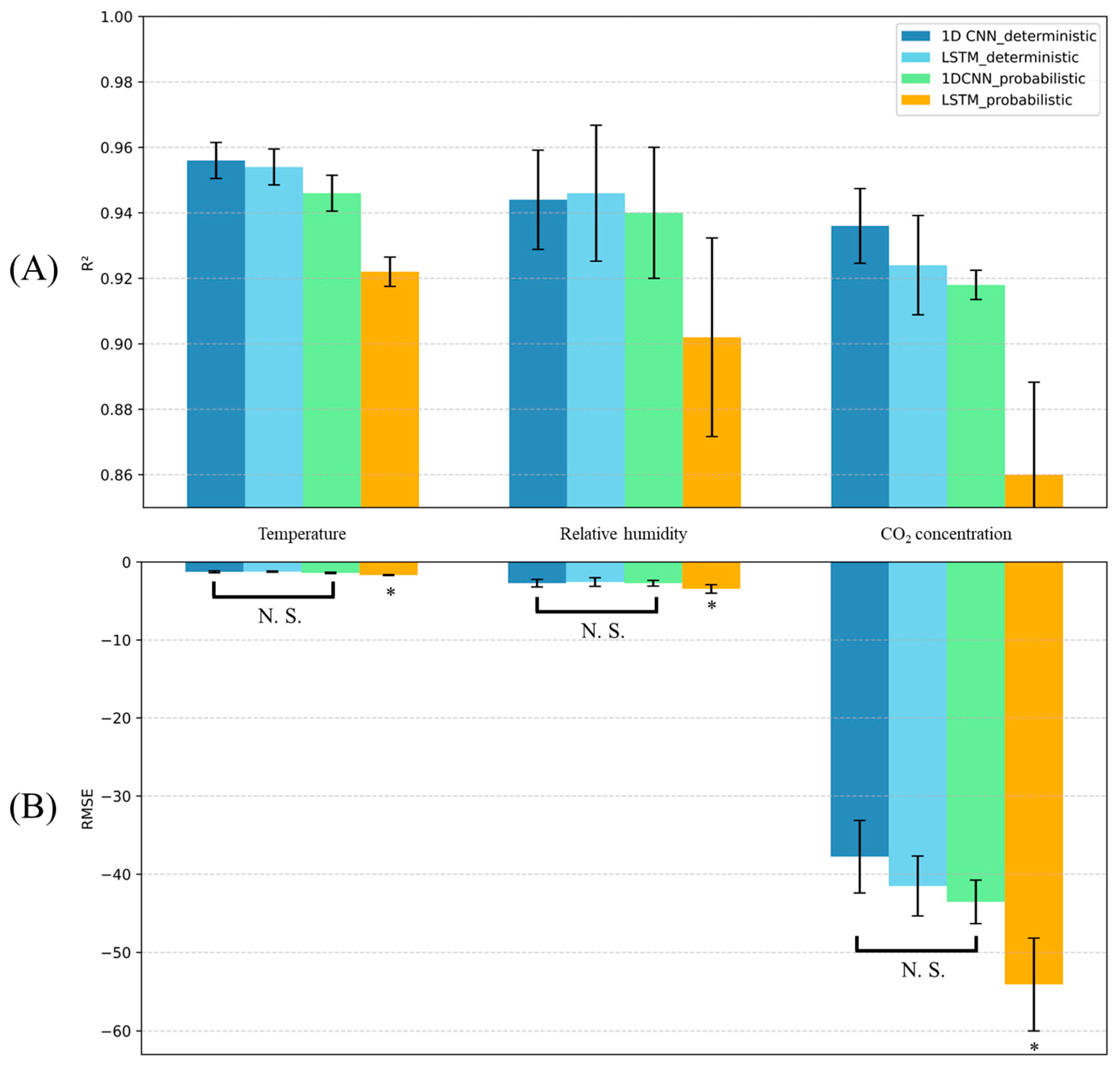
Among the evaluated models, the 1D CNN based probabilistic model demonstrated meaningful performance in predicting the three greenhouse microclimate variables. Although its average R2 values were 0.014 lower than the deterministic 1D CNN model revealed no statistically significant differences in RMSE across time steps (Figure 2). These results indicate that the probabilistic model achieved predictive performance comparable to that of the deterministic model, while also learning to estimate predictive uncertainty quantitatively. The input vector length was optimized for model training and approximation, resulting in reliable results for both microclimate prediction and uncertainty estimation. During training, the model converged based on the NLL loss function (Supplementary Figure S1).
The optimal time series length for model input was 24 h, and detailed performance results of the algorithms used for model comparison across input time lengths are provided in Supplementary Tables S1 and S2. At this time, since the probabilistic model does not provide output for each microclimate variable, the performance for the three variables was comprehensively considered, and therefore the performance weights were set equally. Additionally, we applied sine–cosine encoding to the wind direction variable and compared the model’s performance. Since this pre-processing did not improve the model’s predictive performance, we used the received wind direction data directly as input to the model. To examine whether input lengths longer than 24 h provide additional benefits for capturing periodicity, we evaluated the model performance using the optimal probabilistic 1D CNN with a 48 h input window. However, the 48 h input did not yield any performance improvement compared to the 24 h input. This suggests that the model was able to sufficiently interpret the temporal characteristics of the data using only the 24 h input. Additionally, the model used in this study is lightweight and requires little computation (3.86M FLOPs). Therefore, considering data utilization efficiency and model performance, 24 h was selected as the optimal length for this study.
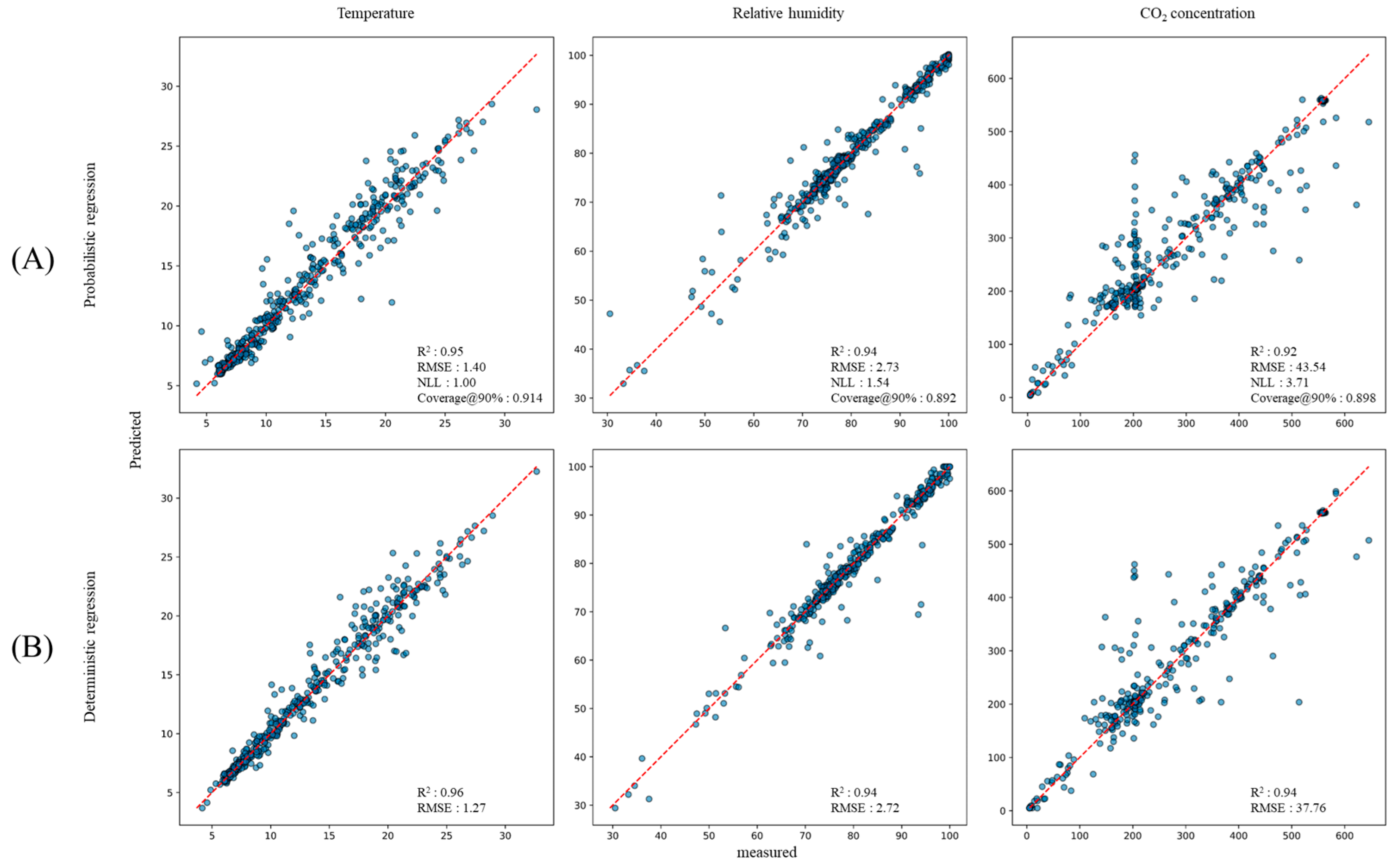
The trained model achieved R2 values of 0.95, 0.94, and 0.92, and RMSE values of 1.4 °C, 2.73%, and 43.54 ppm for internal temperature, relative humidity, and CO2 concentration, respectively. The NLL and Coverage@90% values computed from the output covariance were 1.00, 1.54, and 3.71, and 0.914, 0.892, and 0.898 for the respective variables, internal temperature, internal relative humidity, and CO2 concentration (Figure 3).
In addition, the feature importance analysis using the Permutation Importance method showed that, among the 45 input variables, most features contributed meaningfully to the model output, except for a few control variables, such as the right side window and side curtain, that were scarcely activated during operation. Notably, variations in the internal microclimate (e.g., temperature, humidity, and CO2) exhibited the highest contribution, followed by external weather variables and other control inputs, which demonstrated relatively uniform levels of importance. These findings indicate that the model primarily relies on internal environmental dynamics as key predictive factors, while also integrating external conditions and control signals as supplementary information.

3.2. Quantitative Uncertainty Estimated from the Trained Probabilistic Model

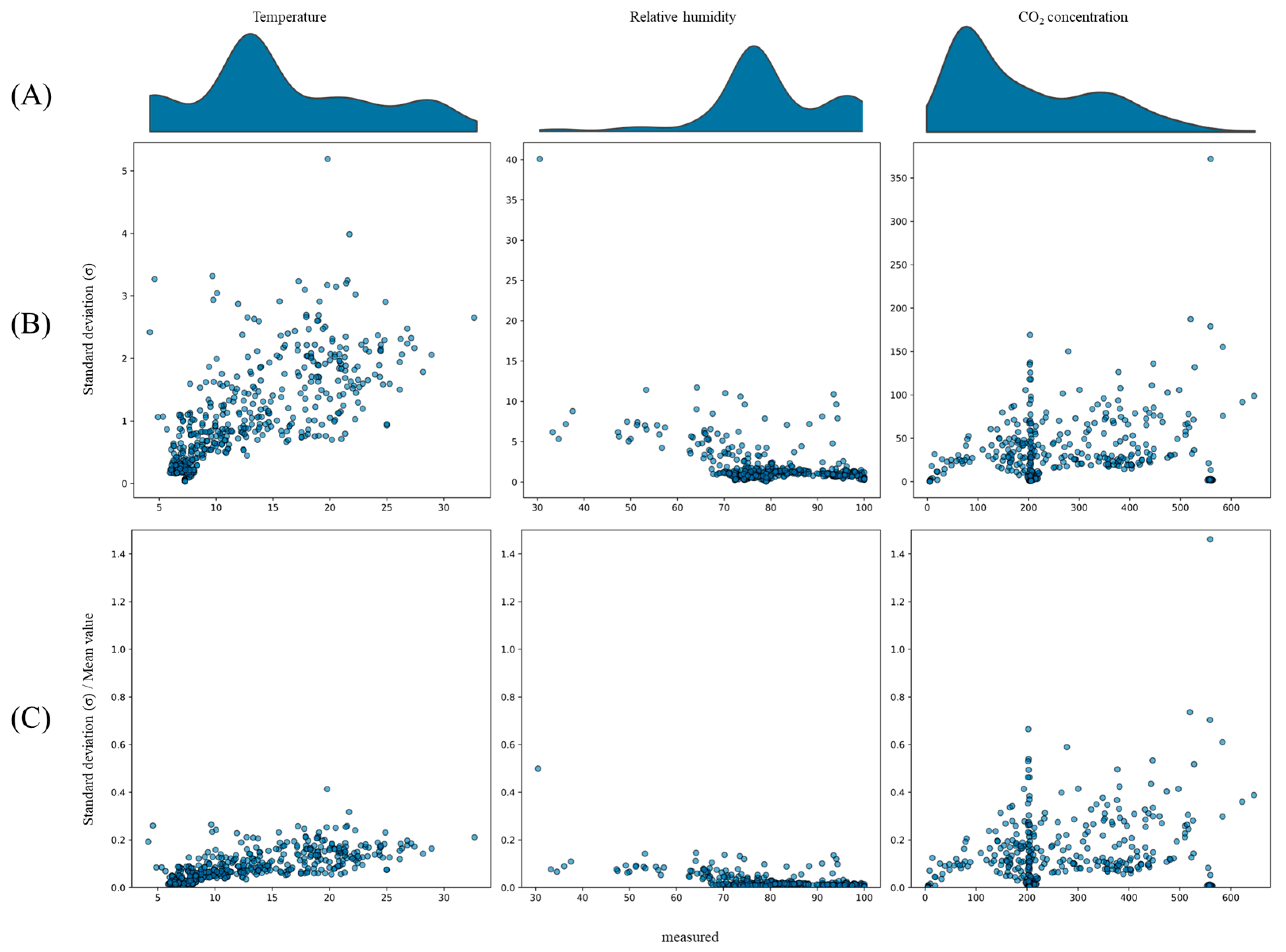
The variance calculated from the model-estimated covariance matrix (Σ) was interpreted using its square root, representing the standard deviation of each prediction ( σ i ). The results exhibited apparent differences depending on the temporal distribution and variable characteristics of the sampled data used during model training. Notably, a significant increase in standard deviation was observed in time intervals with lower sampling frequencies. Moreover, Wald t-tests conducted within the regression framework demonstrated that sampling frequency exerted an independent and statistically significant effect on the variability of the standard deviation (p < 0.001) (Figure 4A,B). Because the absolute magnitude of the standard deviation is highly dependent on the scale and unit of each variable, the values were normalized by dividing them by the respective median values of each variable to enable relative comparison across variables. The predictions for internal temperature and relative humidity exhibited relatively low normalized standard deviations, whereas those for CO2 concentration showed comparatively higher values (Figure 4C).

3.3. Prediction of Time-Varying Correlations Among Microclimate Variables

The correlations between variables computed from the covariance matrices at each time step did not converge, instead exhibiting a wide distribution, indicating the absence of distinct seasonal or temporal patterns (Figure 5A). The average pairwise correlations were 0.23 for temperature–relative humidity, −0.05 for temperature–CO2 concentration, and −0.00 for relative humidity–CO2 concentration (Figure 5B). The range of extreme values nearly covered the entire theoretical limits of the correlation coefficient (−1 to 1) (Figure 5C).

4. Discussion

4.1. Interpretation of Sharpness and Calibration of the Probabilistic Model

The probabilistic algorithm developed in this study simultaneously predicted nine parameters during the learning process. In contrast, the deterministic model, designed for performance comparison, can have a stronger approximation ability because it learns individual prediction branch layer for each microclimate variable through an MTL structure [22]. However, the learning results showed that the probabilistic 1D CNN model exhibited a slight decrease in inference performance compared to the deterministic prediction, although the difference was not statistically significant (Figure 2), as confirmed by the Diebold–Mariano (DM) test applied to the time-series results aggregated from five independent inference evaluations and adjusted using the Holm correction [23,24]. This indicates that the probabilistic model maintained a comparable level of mean predictive accuracy while possessing additional learning flexibility for uncertainty estimation. Therefore, the proposed probabilistic approach serves as an alternative model architecture that can provide both quantitative reliability in prediction and distribution-based interpretability.
The NLL metric used to evaluate uncertainty quantitatively becomes smaller when the predicted values are closer to the observations and when the expected covariance appropriately reflects the scale of actual errors [25]. Accordingly, the NLL value of 2.08 obtained in this study indicates that the variance neither overestimates nor underestimates the actual error magnitude, reasonably representing the uncertainty of the predictions (Figure 3). These results suggest that the model simultaneously achieved sharpness, the degree to which the predictive distribution is narrow and concentrated, representing precision, and calibration, the extent to which the predicted probability distribution aligns with the frequency of observed outcomes, representing reliability [26]. However, because the NLL jointly considers both predictive distributions and variances, it is highly scale-dependent, making it unsuitable for evaluating model performance based on an absolute threshold [27]. Therefore, in this study, the Coverage@90% metric was additionally employed to quantify the reliability of the probabilistic uncertainty estimates. By setting a target confidence level of 0.900, the model’s calibration reliability was assessed, and the resulting Coverage@90% = 0.901, representing the average value across the three variables predicted by the proposed trained model, was highly consistent with the target level, supporting the high reliability of the model’s probabilistic uncertainty estimation (Figure 3) [28].

4.2. Analysis of Uncertainty Distribution in Model Predictions

The greenhouse microclimate data used in this study exhibited nonlinear characteristics and an uneven distribution. Based on the model outputs, the prediction uncertainty was evaluated using the standard deviation. The results showed that regions with lower data frequency tended to produce higher standard deviation values, indicating that the model recognized these regions as areas of greater uncertainty (Figure 4). These results are consistent with previous studies showing that deep learning-based prediction models have poor accuracy or fail to predict in regions with low frequency or unobserved data [29]. Greenhouse and other agricultural datasets inherently contain noise, control-induced events, and external meteorological disturbances, leading to irregularities, errors, and nonlinearities in the data [30]. Therefore, rather than prioritizing the high accuracy of deterministic models that merely approximate future microclimate values, the probabilistic model developed in this study provides rational uncertainty estimation and quantification of confidence intervals. Such characteristics are expected to offer valuable insights into risk management and decision-making in agricultural control strategies.

4.3. Interpretation of Time-Varying Correlations Among Microclimate Variables

The correlations calculated from the model’s output parameters represent the simultaneous variability between variables and interpret the different dynamic relationships at each point in time. These correlations represent the simultaneous variability between variables at each point in time and quantitatively interpret interdependence by reflecting dynamic relationships that change over time [31]. In this study, the correlations between variables exhibited significant temporal variability, and no consistent correlation structure was observed across specific variable pairs. This behavior reflects localized fluctuation patterns and compensates for the limitations of conventional global correlation analyses, in which temporal variations tend to be averaged out or lost [32]. Indeed, the average correlation values derived from the model at each time step cannot explain the distribution of values obtained through global correlation analysis of each variable (Figure 5). This discrepancy arises because global correlation analysis is susceptible to the sampling interval and frequency of the entire time series [33]. When sampling was performed at specific time points and a global correlation analysis was conducted, the resulting correlation values varied substantially (Supplementary Figure S2). In other words, global correlation analysis may be inappropriate, especially in environments with high nonlinear temporal variability, such as those found in greenhouses. Therefore, the temporal correlation used in this study was validated by employing a temporal dynamic correlation matrix that accounts for uncertainty, thereby compensating for the variability of local correlations that are not captured in global correlation analysis. These results are expected to be utilized in designing control strategies that account for temporal variable interactions in greenhouse control systems and in implementing adaptive model predictive control.

4.4. Limitation and Toward Generalizable and Adaptive Greenhouse Micro-Climate Models

This study quantitatively analyzed uncertainty in greenhouse microclimate change by applying a probabilistic deep learning approach to estimating greenhouse microclimate changes. However, because it utilized data from a single cropping season in a specific region, generalization across seasonal variations, greenhouse structures, and crop types is limited [34,35]. In particular, in environments with regional differences in external weather conditions and cultivation management strategies, the prediction model may exhibit performance degradation due to domain shift. Furthermore, the correlations between greenhouse microclimate variables can change due to various biological dynamic variables, such as crop species, growth stage, and crop growth stage. Therefore, Future research should integrate multi-regional and crop interaction data and apply transfer learning or domain adaptation techniques to enhance the model’s generalization ability and robustness [36,37].

5. Conclusions

In this study, we employed a probabilistic deep learning approach to predict changes in greenhouse microclimate. Beyond simple deterministic predictions, we built a robust model capable of quantitatively interpreting and explaining uncertainty. The proposed model can support growers’ stable and reliable control decisions by providing information on the uncertainty and reliability of prediction results, as well as time-varying correlations between variables. These results demonstrate that predictions that account for uncertainty may have more practical implications for risk management and control strategies in actual greenhouse environments than highly accurate predictions expressed in numerical values. However, because this study was based on data collected from a specific region and period, future research is needed to verify the model’s generalizability and to consider nonlinear variability across growth stages. Additionally, the probabilistic model developed in this study can be extended to an explainable and stable predictive control framework by integrating it into real-time model-based control.

Supplementary Materials

The following supporting information can be downloaded at: https://www.mdpi.com/article/10.3390/agriculture15232461/s1, Table S1: Greenhouse microclimate prediction performance of a probabilistic model as a function of input vector length. Prediction performance represents the average of performance derived from five fixed random seed iterations. The displayed prediction performance represents, from top to bottom, the performance of internal temperature, internal relative humidity, and CO2 concentration variables. RMSE units are omitted (°C, %, ppm, respectively), Table S2: Greenhouse microclimate prediction performance according to the length of the input vector of a deterministic model. The format of the prediction performance is as shown in Supplementary Table S1, Figure S1. NLL loss curves over 1000 epochs for both the training and validation datasets during the training of the probabilistic 1D CNN model, Figure S2. Global correlations between greenhouse microclimate variables calculated from data obtained from two random states; 3 (A); 240707 (B).

Author Contributions

Conceptualization, W.-J.C. and M.Y.; methodology, W.-J.C. and M.Y.; software, W.-J.C.; validation, W.-J.C. and M.Y.; formal analysis, W.-J.C.; investigation, W.-J.C.; resources, W.-J.C. and M.Y.; data curation, W.-J.C.; writing—original draft preparation, W.-J.C.; writing—review and editing, M.Y.; visualization, W.-J.C.; supervision, M.Y.; project administration, M.Y.; funding acquisition, M.Y. All authors have read and agreed to the published version of the manuscript.

Funding

This work was supported by Korea Institute of Planning and Evaluation for Technology in Food, Agriculture and Forestry (IPET) and Korea Smart Farm R&D Foundation (KosFarm) through Smart Farm Innovation Technology Development Program, funded by Ministry of Agriculture, Food and Rural Affairs (MAFRA) and Ministry of Science and ICT (MSIT), Rural Development Administration (RDA) (RS-2024-00399854).

Institutional Review Board Statement

Not applicable.

Data Availability Statement

The original contributions presented in this study are included in the article/Supplementary Materials. Further inquiries can be directed to the corresponding author.

Conflicts of Interest

The authors declare no conflicts of interest.

References

  1. Sánchez-Molina, J.; Perez, N.; Rodríguez, F.; Guzmán, J.; López, J. Support system for decision making in the management of the greenhouse environmental based on growth model for sweet pepper. Agric. Syst. 2015, 139, 144–152. [Google Scholar] [CrossRef]
  2. Hemming, S.; Zwart, F.d.; Elings, A.; Petropoulou, A.; Righini, I. Cherry tomato production in intelligent greenhouses—Sensors and AI for control of climate, irrigation, crop yield, and quality. Sensors 2020, 20, 6430. [Google Scholar] [CrossRef]
  3. Chen, S.; Liu, A.; Tang, F.; Hou, P.; Lu, Y.; Yuan, P. A Review of Environmental Control Strategies and Models for Modern Agricultural Greenhouses. Sensors 2025, 25, 1388. [Google Scholar] [CrossRef]
  4. Petrakis, T.; Kavga, A.; Thomopoulos, V.; Argiriou, A.A. Neural network model for greenhouse microclimate predictions. Agriculture 2022, 12, 780. [Google Scholar] [CrossRef]
  5. Sun, W.; Chang, F.-J. Empowering greenhouse cultivation: Dynamic factors and machine learning unite for advanced microclimate prediction. Water 2023, 15, 3548. [Google Scholar] [CrossRef]
  6. Ajani, O.S.; Usigbe, M.J.; Aboyeji, E.; Uyeh, D.D.; Ha, Y.; Park, T.; Mallipeddi, R. Greenhouse micro-climate prediction based on fixed sensor placements: A machine learning approach. Mathematics 2023, 11, 3052. [Google Scholar] [CrossRef]
  7. Shi, D.; Yuan, P.; Liang, L.; Gao, L.; Li, M.; Diao, M. Integration of deep learning and sparrow search algorithms to optimize greenhouse microclimate prediction for seedling environment suitability. Agronomy 2024, 14, 254. [Google Scholar] [CrossRef]
  8. Fink, M.; Daniels, A.; García-Mañas, F.; Rodríguez, F.; Leibold, M.; Wollherr, D. Learning-based model identification for greenhouse climate control. at-Automatisierungstechnik 2025, 73, 451–465. [Google Scholar] [CrossRef]
  9. Yu, J.; Sun, C.; Zhao, J.; Ma, L.; Zheng, W.; Xie, Q.; Wei, X. Prediction and control of greenhouse temperature: Methods, applications, and future directions. Comput. Electron. Agric. 2025, 237, 110603. [Google Scholar] [CrossRef]
  10. Ajagekar, A.; Mattson, N.S.; You, F. Energy-efficient ai-based control of semi-closed greenhouses leveraging robust optimization in deep reinforcement learning. Adv. Appl. Energy 2023, 9, 100119. [Google Scholar] [CrossRef]
  11. Mallick, S.; Airaldi, F.; Dabiri, A.; Sun, C.; De Schutter, B. Reinforcement learning-based model predictive control for greenhouse climate control. Smart Agric. Technol. 2025, 10, 100751. [Google Scholar] [CrossRef]
  12. Mahmood, F.; Govindan, R.; Bermak, A.; Yang, D.; Al-Ansari, T. Data-driven robust model predictive control for greenhouse temperature control and energy utilisation assessment. Appl. Energy 2023, 343, 121190. [Google Scholar] [CrossRef]
  13. Chen, W.-H.; You, F. Efficient greenhouse temperature control with data-driven robust model predictive. In Proceedings of the 2020 American Control Conference (ACC), Denver, CO, USA, 1–3 July 2020; pp. 1986–1991. [Google Scholar]
  14. Zhong, L.; Guo, X.; Ding, M.; Ye, Y.; Jiang, Y.; Zhu, Q.; Li, J. SHAP values accurately explain the difference in modeling accuracy of convolution neural network between soil full-spectrum and feature-spectrum. Comput. Electron. Agric. 2024, 217, 108627. [Google Scholar] [CrossRef]
  15. Bansal, A.; Balaji, K.; Lalani, Z. Temporal encoding strategies for energy time series prediction. arXiv 2025, arXiv:2503.15456. [Google Scholar] [CrossRef]
  16. Ahn, J.Y.; Kim, Y.; Park, H.; Park, S.H.; Suh, H.K. Evaluating Time-Series Prediction of Temperature, Relative Humidity, and CO2 in the Greenhouse with Transformer-Based and RNN-Based Models. Agronomy 2024, 14, 417. [Google Scholar] [CrossRef]
  17. Ishida, K.; Ercan, A.; Nagasato, T.; Kiyama, M.; Amagasaki, M. Use of 1D-CNN for input data size reduction of LSTM in Hourly Rainfall-Runoff modeling. arXiv 2021, arXiv:2111.04732. [Google Scholar]
  18. Hochreiter, S.; Schmidhuber, J. Long short-term memory. Neural Comput. 1997, 9, 1735–1780. [Google Scholar] [CrossRef]
  19. Kiranyaz, S.; Ince, T.; Gabbouj, M. Real-time patient-specific ECG classification by 1-D convolutional neural networks. IEEE Trans. Biomed. Eng. 2015, 63, 664–675. [Google Scholar] [CrossRef]
  20. Rangapuram, S.S.; Seeger, M.W.; Gasthaus, J.; Stella, L.; Wang, Y.; Januschowski, T. Deep state space models for time series forecasting. In Proceedings of the 32nd International Conference on Neural Information Processing Systems, Montréal, QC, Canada, 3–8 December 2018; Volume 31. [Google Scholar]
  21. Salinas, D.; Flunkert, V.; Gasthaus, J.; Januschowski, T. DeepAR: Probabilistic forecasting with autoregressive recurrent networks. Int. J. Forecast. 2020, 36, 1181–1191. [Google Scholar] [CrossRef]
  22. Aoki, R.; Tung, F.; Oliveira, G.L. Heterogeneous multi-task learning with expert diversity. IEEE/ACM Trans. Comput. Biol. Bioinform. 2022, 19, 3093–3102. [Google Scholar] [CrossRef]
  23. Diebold, F.X.; Mariano, R.S. Comparing predictive accuracy. J. Bus. Econ. Stat. 2002, 20, 134–144. [Google Scholar] [CrossRef]
  24. Holm, S. A simple sequentially rejective multiple test procedure. Scand. J. Stat. 1979, 6, 65–70. [Google Scholar]
  25. Lakshminarayanan, B.; Pritzel, A.; Blundell, C. Simple and scalable predictive uncertainty estimation using deep ensembles. In Proceedings of the 31st International Conference on Neural Information Processing Systems, Long Beach, CA, USA, 4–9 December 2017; Volume 30. [Google Scholar]
  26. Gneiting, T.; Balabdaoui, F.; Raftery, A.E. Probabilistic forecasts, calibration and sharpness. J. R. Stat. Soc. Ser. B Stat. Methodol. 2007, 69, 243–268. [Google Scholar] [CrossRef]
  27. Ovadia, Y.; Fertig, E.; Ren, J.; Nado, Z.; Sculley, D.; Nowozin, S.; Dillon, J.; Lakshminarayanan, B.; Snoek, J. Can you trust your model’s uncertainty? evaluating predictive uncertainty under dataset shift. In Proceedings of the 33rd International Conference on Neural Information Processing Systems, Vancouver, BC, Canada, 8–14 December 2019; Volume 32. [Google Scholar]
  28. Kuleshov, V.; Fenner, N.; Ermon, S. Accurate uncertainties for deep learning using calibrated regression. In Proceedings of the International Conference on Machine Learning, Stockholm, Sweden, 10–15 July 2018; pp. 2796–2804. [Google Scholar]
  29. Malinin, A.; Gales, M. Reverse KL-divergence training of prior networks: Improved uncertainty and adversarial robustness. In Proceedings of the 33rd International Conference on Neural Information Processing Systems, Vancouver, BC, Canada, 8–14 December 2019; Volume 32. [Google Scholar]
  30. Ma, D.; Carpenter, N.; Maki, H.; Rehman, T.U.; Tuinstra, M.R.; Jin, J. Greenhouse environment modeling and simulation for microclimate control. Comput. Electron. Agric. 2019, 162, 134–142. [Google Scholar] [CrossRef]
  31. Hafner, C.M.; Franses, P.H. A Generalized Dynamic Conditional Correlation Model for Many Asset Returns. 2003. Available online: https://repub.eur.nl/pub/1718/feweco20030708113101.pdf (accessed on 27 October 2025).
  32. Ding, Z.; Granger, C.W. Modeling volatility persistence of speculative returns: A new approach. J. Econom. 1996, 73, 185–215. [Google Scholar] [CrossRef]
  33. Granger, C.W.; Weiss, A.A. Time series analysis of error-correction models. In Studies in Econometrics, Time Series, and Multivariate Statistics; Elsevier: Amsterdam, The Netherlands, 1983; pp. 255–278. [Google Scholar]
  34. Bakker, J.; Bot, G.; Challa, H.; Van de Braak, N. Greenhouse Climate Control: An Integrated Approach; Wageningen Academic Publishers: Wageningen, The Netherlands, 1995. [Google Scholar]
  35. Eraliev, O.; Lee, C.-H. Performance analysis of time series deep learning models for climate prediction in indoor hydroponic greenhouses at different time intervals. Plants 2023, 12, 2316. [Google Scholar] [CrossRef]
  36. Wang, M.; Deng, W. Deep visual domain adaptation: A survey. Neurocomputing 2018, 312, 135–153. [Google Scholar] [CrossRef]
  37. Kumar, P.; Chandra, R.; Bansal, C.; Kalyanaraman, S.; Ganu, T.; Grant, M. Micro-climate prediction-multi scale encoder-decoder based deep learning framework. In Proceedings of the 27th ACM SIGKDD Conference on Knowledge Discovery & Data Mining, Virtual, 14–18 August 2021; pp. 3128–3138. [Google Scholar]
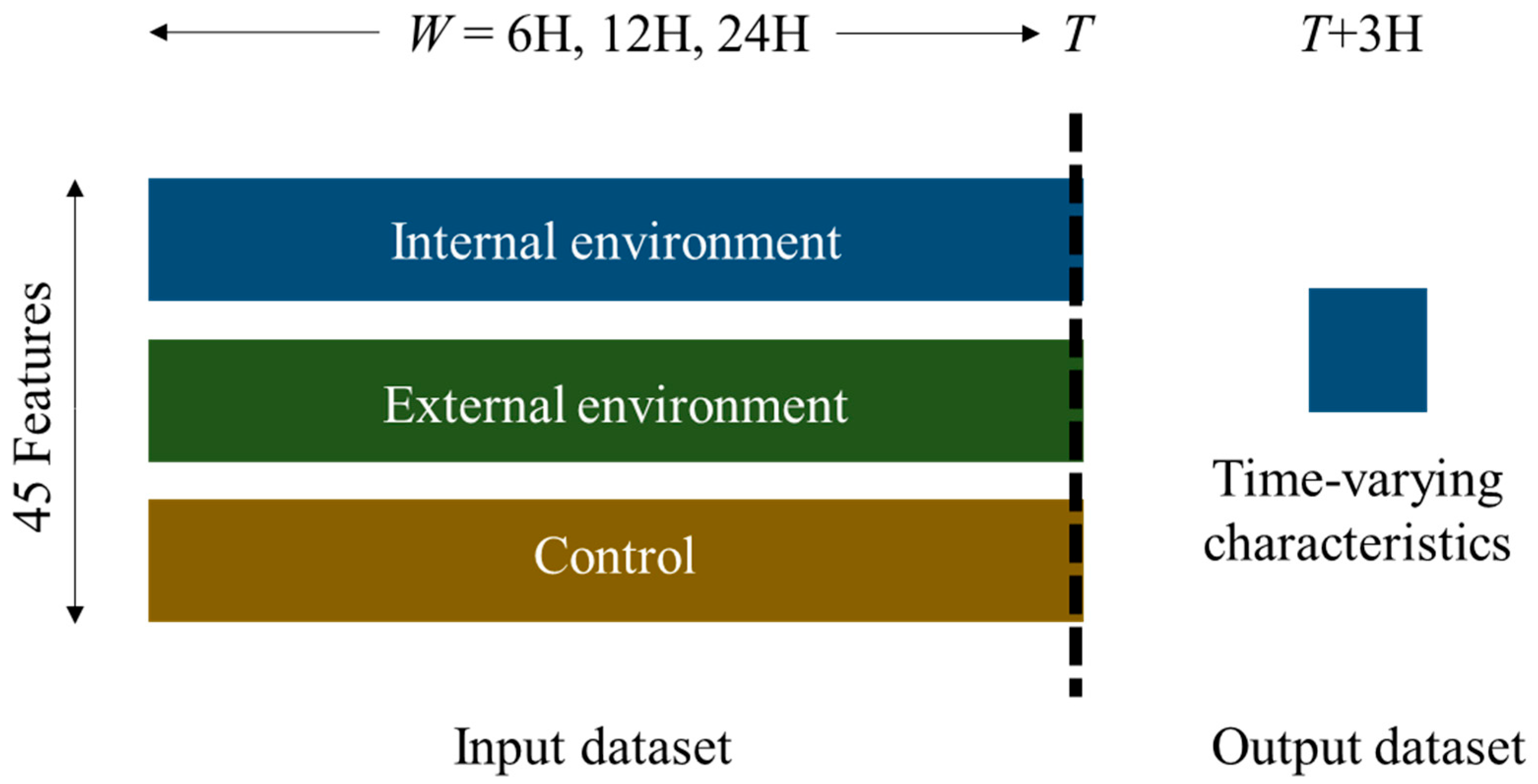
Figure 1. Schematic overview of the input–output dataset construction based on the sliding window method using the collected time-series greenhouse internal, external environmental, and control data. The sliding window method was employed to construct training datasets for predicting future microclimate time-varying characteristic variables from past input sequences of internal environment, external environment data, and control with length of W.
Agriculture 15 02461 g001
Figure 2. Comparative performance results of the four models for greenhouse microclimate prediction. (A) presents the R2 performance of each model, and (B) shows the mean RMSE across time steps visualized as bar plots. The results of the DM test for time-step statistical analysis are also indicated in (B). The 1D CNN probabilistic model had slightly lower prediction performance than the deterministic model, but there was no statistically significant difference in the DM test based on the RMSE of five random states and seeds (N.S.). The p-values for temperature, relative humidity, and CO2 concentration were 0.155, 1.000, and 0.067 for the 1D CNN deterministic model, and 0.155, 1.000, and 0.177 for the LSTM deterministic model, respectively. At this time, the probabilistic LSTM showed significantly lower performance (p-values < 0.05), which is marked with an asterisk (*) in (B).
Agriculture 15 02461 g002
Figure 3. Comparison of greenhouse microclimate prediction results. (A,B) show the predictions of the probabilistic 1D CNN model and the deterministic 1D CNN model, respectively, for the three microclimate variables, temperature, relative humidity, and CO2 concentration, in comparison with the observed values. All results include the R2 and RMSE, while the probabilistic model additionally reports the NLL and Coverage@90% metrics.
Agriculture 15 02461 g003
Figure 4. Distribution of the standard deviations calculated from the covariance outputs of the probabilistic 1D CNN model. (A) shows the data density within the observed range, while (B) presents the distribution of standard deviations across the same range. (C) illustrates the distribution of normalized standard deviations obtained by dividing each variable’s standard deviation by its respective median value.
Agriculture 15 02461 g004
Figure 5. Distribution of correlations between variables calculated from a time-varying covariance matrix. (A) shows the temporal evolution of correlations for each pair of variables, (B) shows the frequency distribution of correlation values, and (C) shows statistical characteristics represented as boxplots. The red dashed line and solid line in the figure indicate the mean position of each correlation.
Agriculture 15 02461 g005
Table 1. Types, measurement ranges and number of outliers of the collected greenhouse microclimate, external environment, and control data. The range of each variable represents its temporal variability and the operational range of the corresponding sensors.
FactorValuesOutlier
Internal temperature (°C)2.75 to 32.6718
Internal relative humidity (%)28.92 to 99.3337
Internal CO2 concentration (ppm)120.5 to 67123
External temperature (°C)−10.4 to 28.311
External relative humidity (%)16 to 10017
Precipitation (mm)0 to 45.30
Wind speed (m/s)0 to 6.79
Wind direction (°)0 to 3600
Radiation (W/m2)0 to 850.8339
Snowfall (cm)0 to 5.70
Ground temperature (°C)−8 to 42.723
Up window (left, right—01 to 04) (%)0, 50, 1000
Side window (left, right—01 to 04) (%)0, 50, 1000
Curtain (up, down, left, right—01 to 04) (%)0, 50, 1000
Table 2. Network architectures of the LSTM and 1D CNN models for probabilistic prediction. Dense represents a fully connected layer. The parameters are denoted as ‘layer type (number of nodes)’. In the input size notation, N refers to the batch size and W indicates the input vector length, which was tested with three different configurations during model training.
AlgorithmLSTM Probabilistic1D CNN Probabilistic
Input size(N, W, 45)
Hidden layersLSTM (128)
Layer normalization
LSTM (128)
Layer normalization
Global average pooling
Dense (512)
Dense (512)
1D Conv (128)
Batch normalization
Spatial dropout
1D Conv (128)
Batch normalization
Spatial dropout
Global average pooling
Dense (512)
Dense (512)
outputsDense (9)Dense (9)
Table 3. Network architectures of the LSTM and 1D CNN models for deterministic prediction. The detailed parameter configurations of each model are provided in Table 2. The MTL layer was implemented to predict three greenhouse microclimate variables, temperature, relative humidity, and CO2 concentration, and employed identical substructures for each variable.
AlgorithmLSTM Deterministic1D CNN Deterministic
Input size(N, W, 45)
Hidden layersLSTM (128)
Layer normalization
LSTM (128)
Layer normalization
Global average pooling
1D Conv (128)
Batch normalization
Spatial dropout
1D Conv (128)
Batch normalization
Spatial dropout
Global average pooling
MTLDense (128)
Dense (128)
Dense (128)
Dense (128)
Dense (128)
Dense (128)
Dense (128)
Dense (128)
Dense (128)
Dense (128)
Dense (128)
Dense (128)
outputsDense
(1)
Dense
(1)
Dense
(1)
Dense
(1)
Dense
(1)
Dense
(1)
Disclaimer/Publisher’s Note: The statements, opinions and data contained in all publications are solely those of the individual author(s) and contributor(s) and not of MDPI and/or the editor(s). MDPI and/or the editor(s) disclaim responsibility for any injury to people or property resulting from any ideas, methods, instructions or products referred to in the content.