UAV-Based Multimodal Monitoring of Tea Anthracnose with Temporal Standardization

Abstract

Tea Anthracnose (TA), caused by fungi of the genus Colletotrichum, is one of the major threats to global tea production. UAV remote sensing has been explored for non-destructive and high-efficiency monitoring of diseases in tea plantations. However, variations in illumination, background, and meteorological factors undermine the stability of cross-temporal data. Data processing and modeling complexity further limits model generalizability and practical application. This study introduced a cross-temporal, generalizable disease monitoring approach based on UAV multimodal data coupled with relative-difference standardization. In an experimental tea garden, we collected multispectral, thermal infrared, and RGB images and extracted four classes of features: spectral (Sp), thermal (Th), texture (Te), and color (Co). The Normalized Difference Vegetation Index (NDVI) was used to identify reference areas and standardize features, which significantly reduced the relative differences in cross-temporal features. Additionally, we developed a vegetation–soil relative temperature (VSRT) index, which exhibits higher temporal-phase consistency than the conventional normalized relative canopy temperature (NRCT). A multimodal optimal feature set was constructed through sensitivity analysis based on the four feature categories. For different modality combinations (single and fused), three machine learning algorithms, K-Nearest Neighbors (KNN), Support Vector Machine (SVM), and Multi-layer Perceptron (MLP), were selected to evaluate disease classification performance due to their low computational burden and ease of deployment. Results indicate that the “Sp + Th” combination achieved the highest accuracy (95.51%), with KNN (95.51%) outperforming SVM (94.23%) and MLP (92.95%). Moreover, under the optimal feature combination and KNN algorithm, the model achieved high generalizability (86.41%) on independent temporal data. This study demonstrates that fusing spectral and thermal features with temporal standardization, combined with the simple and effective KNN algorithm, achieves accurate and robust tea anthracnose monitoring, providing a practical solution for efficient and generalizable disease management in tea plantations.

1. Introduction

Tea anthracnose (TA), caused by fungi of the genus Colletotrichum, is one of the most damaging foliar diseases affecting global tea production [1]. In the early stages of the disease, small water-soaked spots appear on leaves, which subsequently develop into dark brown necrotic lesions that ultimately lead to leaf tissue necrosis, graying, and distortion [2,3]. It is distributed across all major tea-producing regions in China, with large-scale outbreaks particularly prevalent during hot and rainy seasons. Its incidence rate in the field can reach 30–50% [1]. Infected tea gardens often develop distinct centers of infection, which in severe cases can cause extensive defoliation and significantly reduce both tea yield and quality [4]. Therefore, it is crucial to monitor and control this disease. Currently, tea garden disease monitoring primarily relies on manual inspections, which suffer from drawbacks such as high subjectivity, low efficiency, and limited spatial coverage [5]. For tea gardens in mountainous areas characterized by small plots and high landscape fragmentation, traditional ground-based sampling methods struggle to support routine inspections and large-scale dynamic monitoring.

With the advancement of agricultural remote sensing technology, new research has focused on the use of satellite or unmanned aerial vehicle (UAV)-based remote sensing for monitoring crop pests and diseases [6]. Although satellite remote sensing provides extensive coverage capabilities, it is constrained by low spatial resolution, long revisit intervals, and susceptibility to weather [7]. These limitations make it difficult to meet the fine-scale monitoring requirements of tea fields that are small and structurally complex. In contrast, UAV remote sensing has emerged as an ideal platform for tea garden disease monitoring due to its high spatio-temporal resolution, high efficiency and flexibility, as well as low cost [8]. Equipped with multispectral, thermal infrared, hyperspectral, RGB, and other sensors, UAVs capture multidimensional information on crop stress [9]. For example, Bhandari et al. assessed the severity of winter wheat foliage disease using UAV RGB imagery combined with linear regression, achieving correlation coefficient squared (R²) values as high as 0.86 [10]. Su et al. monitored wheat yellow rust by combining UAV multispectral data with a random forest algorithm, attaining an overall accuracy of 89.3% [11]. Abdulridha et al. employed UAV-based hyperspectral imaging to monitor target spots and bacterial spot diseases in tomato, achieving a classification accuracy of up to 99% for both diseases [12]. Compared to RGB and multispectral imaging, hyperspectral data offers higher precision but there are high data acquisition and processing costs in large-scale applications. Additionally, studies based on UAV thermal infrared data have demonstrated the use for disease detection [13], yet applications integrating it with other modalities are relatively scarce. Overall, most existing studies have focused on single-modality data processing and modeling, with limited exploration of multimodal data fusion. This constrains the model accuracy and cross-temporal generalization.

Recently, some researchers have attempted to fuse multimodal remote sensing information, such as spectral, temperature, texture, and color for crop stress monitoring, to better capture the multidimensional responses induced by stress [9,14]. By capitalizing on multimodal complementarity, we can capture disease-related physiological and structural changes at remote sensing scales (e.g., chlorophyll depletion, altered stomatal conductance, heightened texture heterogeneity, and elevated canopy temperature), which improves the accuracy of stress monitoring and the robustness of cross-temporal application [15,16]. For instance, Ma et al. used machine learning models to combine spectral, textural, and color features extracted from UAV multispectral and RGB imagery [17]. They estimated the severity of cotton verticillium wilt at different growth stages, achieving significantly higher accuracy than using spectral features alone. Liu et al. extracted spectral, texture, and temperature features from UAV multispectral and thermal images built multiple linear regression models to estimate disease severity of wheat powdery mildew at different infection stages, achieving a maximum R² of 0.90 [18]. Liu et al. extracted spectral and texture features from UAV-based hyperspectral data and developed a rice blast disease classification model using a Transform network, achieving a maximum classification accuracy of 96.98% [19]. These studies have demonstrated the effectiveness of combining multi-source features for crop monitoring, including cotton, wheat, and rice. However, research on the monitoring of tea tree anthracnose remains relatively limited. In particular, although existing studies have achieved significant results in disease monitoring accuracy, there is still a lack of exploration into simple data processing methods, the development of easily deployable monitoring models, and improvements in model generalization and versatility, especially within the context of routine tea garden disease monitoring.

Additionally, temporal phase differences continue to be a primary bottleneck in conducting regular and efficient inspections because they interfere with disease feature identification and weaken model generalization. In multi-temporal monitoring, differences in UAV acquisition conditions (illumination, weather, temperature, humidity, etc.) and sensor performance often cause significant differences in the appearance of the same land features across different temporal datasets. For example, changes in illumination cause radiance shifts [20], and fluctuations in temperature and humidity affect vegetation thermal radiative properties [21,22]. Such inconsistencies introduce noise that can mask disease signals, significantly reduce the diagnostic capability of key features, and weaken cross-temporal model generalization [23]. Previous studies have shown that relative radiometric normalization using pseudo-invariant feature (PIF) matching on satellite imagery can reduce radiometric differences under varying conditions or from different sensors [24]. However, this approach requires complex and cumbersome identification of invariant regions and its applicability at the UAV scale remains to be validated. Additionally, other studies have demonstrated that texture features constructed from normalized UAV hyperspectral data can mitigate the impact of environmental variations [19], but a standardized method for processing multimodal features across different sensor types is still lacking.

To address these issues in the context of routine, efficient inspections in smart tea plantations, this study proposed a cross-temporal, general monitoring approach for tea anthracnose that combines UAV multimodal remote sensing with relative-difference standardization. The primary objectives included (1) proposing a relative-difference standardization processing workflow based on NDVI to select healthy regions as a reference and address feature temporal inconsistency; (2) extraction and optimization of spectral (Sp), thermal (Th), texture (Te), and color (Co) features through sensitivity analysis to construct a multimodal feature set; (3) evaluation of single and multimodal feature combinations using representative models such as k-nearest neighbors (KNN), support vector machine (SVM), and multi-layer perceptron (MLP), and building a tea anthracnose monitoring model for cross-temporal generalization.

2. Materials and Methods

2.1. Study Area

The study area is located in the experimental tea plantation of Lanxi City, Jinhua, Zhejiang Province, China (119°28′33″ E, 29°6′38″ N) (Figure 1). The region experiences a subtropical monsoon climate, characterized by warm and humid conditions with distinct seasons. Summers and autumns are hot, while winters and springs tend to be relatively cold, with notable rainy and drought periods during the plum rain and summer drought seasons. The dominant tea variety is the anthracnose-susceptible cultivar “Longjing 43,” covering an area of approximately 2.3 km². Due to the ecological management practices in place, anthracnose disease occurs throughout the year in the tea plantation, with the plum rain period and autumn, marked by heavy rainfall, being particularly severe. The autumn season is the peak period for disease outbreaks. In severely affected areas, distinct disease centers and large quantities of yellow-brown leaves can be observed, which pose a serious threat to both the yield and quality of tea.

2.2. Ground Data Acquisition

Two representative plots with natural occurrences of tea anthracnose were selected in the study area, and ground surveys were conducted during high-incidence periods on 12 and 23 October 2024, as well as 10 October 2025. The surveys employed a DJI Mavic 3T (M3T, Shenzhen DJI Innovation Technology Co., Ltd., Shenzhen, China) UAV equipped with high-precision real-time kinematic (RTK). Random sampling points were chosen within the survey area to collect near-ground RGB images (observation altitude 4 m; 7× telephoto lens). Under the supervision of experienced tea pathologists, trained annotators conducted visual assessments to delineate diseased and healthy canopy areas. To ensure labeling reliability, cross-validation among annotators was performed, and ambiguous samples were re-evaluated through field inspections. The corresponding GPS coordinates of validated samples were then extracted for subsequent multimodal data analysis. Sample counts for each acquisition time are listed in

Table 1. The number of sample points at different periods.

	Data	Healthy	Disease	Total
Temporal Phase 1 (T1)	12 October 2024	104	80	184
Temporal Phase 2 (T2)	23 October 2024	84	120	204
Temporal Phase 3 (T3)	10 October 2025	96	88	184
		284	288	572

.

2.3. UAV Multi-Source Image Acquisition and Preprocessing

In this study, multispectral and RGB data were acquired using the DJI Mavic 3M (M3M, Shenzhen DJI Innovation Technology Co., Ltd., Shenzhen, China) UAV platform, and thermal infrared data were collected with a DJI Mavic 3T (M3T) UAV. The primary payload parameters for both UAVs are detailed in

Table 2. Main payload parameters for UAV.

	Sensors	Spectral Region (μm)	Image Resolution (Pixels)	Equivalent Focal Length (mm)	Diagonal Field of View (D°)	RTK Accuracy	Weight (g)
M3M	RGB	/	5280 × 3956	24	84°	Horizontal: 1 cm + 1 ppm; Vertical: 1.5 cm + 1 ppm	951 (Propeller + RTK module)
	MS	Green: 0.560 ± 0.016	2592 × 1944	25	73.91°
		Red: 0.650 ± 0.016
		RedEdge: 0.730 ± 0.016
		NIR: 0.860 ± 0.026
M3T	RGB-Tele	/	4000 × 3000	162	15°
	TIR	8.0–14.0	640 × 512	40	61°		920 (Propeller)

. Remote sensing data acquisition was conducted concurrently with ground surveys and carried out along preplanned flight lines between 11:00 and 14:00 under clear skies and low-wind conditions. The two UAVs collected sequential multi-source data over the study plots, with flight parameters set to an altitude of 50 m, a speed of 4 m/s, a side overlap of 70%, and a front overlap of 80%.

The multispectral and RGB data from the M3M were orthomosaicked and radiometrically calibrated using DJI Terra v3.5 (Shenzhen DJI Innovation Technology Co., Ltd., Shenzhen, China). Thermal-infrared data from the M3T were converted to temperature values using DJI Thermal SDK v1.5 and orthomosaicked in Agisoft Metashape 2.1 (Agisoft Co., Ltd., St. Petersburg, Russia). Subsequently, geometric correction and image registration were conducted using ENVI 5.3, and then images were clipped to the boundaries of the study plots. To avoid interference from non-tea areas in subsequent analyses, a decision-tree model was constructed in ENVI using the RedEdge band of the multispectral imagery to extract the tea-row regions within the study plots.

2.4. Data Analysis

2.4.1. Spectral, Color, Texture, and Thermal Feature Extraction for Tea Plantations

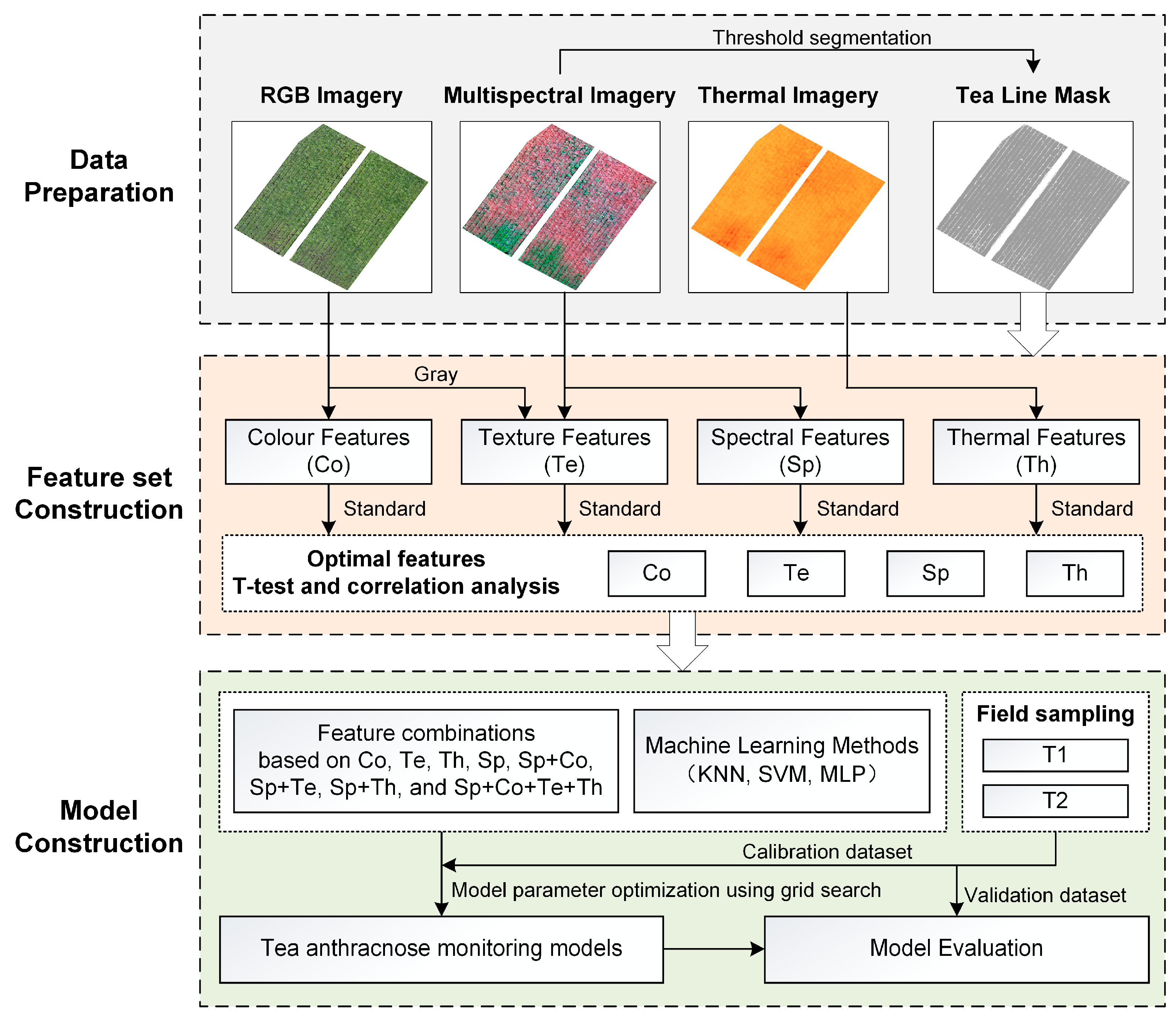
Infection by tea anthracnose causes changes to leaf morphology (curling), color (yellowing), physiological and biochemical composition, as well as transpiration and water status (wilting). These directly or indirectly affect multiple remote sensing signals from the tea canopy [25]. To assess multidimensional tea-plant information, this study extracted four types of features (Sp, Th, Te and Co) from multispectral, thermal infrared, and RGB imagery (Figure 2) and assembled a multimodal feature set for tea anthracnose monitoring.

Spectral features were extracted from UAV multispectral imagery. In addition to the original four bands (Green, Red, RedEdge, and NIR), 17 vegetation indices related to vegetation stress from pests and diseases were selected. These indices are commonly used to characterize leaf area (NDRE, GNDVI), biomass (NDVI), and pigments (CIG, CARI), as shown in Table 3.

Color features were extracted from the RGB imagery, including normalized red (R), green (G), and blue (B) channels and 9 color indices computed from their combinations. Normalized digital number (DN) values were calculated by dividing each channel DN by the sum of the three channels, as given in Equations (1)–(3). In contrast to spectral band-based vegetation indices, the color indices were constructed from normalized R, G, and B values to emphasize attributes like canopy greenness and color contrast for assessing canopy conditions from visible-light information [17,26]. For example, indices such as ExG, RGBVI, and MGRVI have been used to evaluate tea growth status [14]:

$$r=R∕\left(R+G+B\right)$$

(1)

$$g=G∕\left(R+G+B\right)$$

(2)

$$b=B∕\left(R+G+B\right)$$

(3)

where R, G, and B represent the DN values of the three color channels, and r, g, and b represent the normalized standardized values.

Texture features originated from two sources: (i) the RGB grayscale image; and (ii) the multispectral Green, Red, RedEdge, and NIR bands. The Gray-Level Co-occurrence Matrix (GLCM) algorithm in ENVI 5.3 was applied to compute eight texture parameters for each data source [17]. The analysis was conducted using a 3 × 3 window size with a step size of 1 in both the x and y directions. The eight texture parameters include: Mean (MEA), Variance (VAR), Homogeneity (HOM), Contrast (CON), Dissimilarity (DIS), Entropy (ENT), Second Moment (SEC), and Correlation (COR). These parameters were combined in three ways to form texture indices (Table 4), and the potential of texture information for tea anthracnose monitoring was evaluated, with formulas given in Equations (4)–(6). These indices emphasize gray-level variation between adjacent pixels to capture the texture differences induced by lesions in RGB and multispectral imagery [27,28].

$$NDTI=({TP}_1-{TP}_2)∕\left({TP}_1+{TP}_2\right)$$

(4)

$$DTI={TP}_1-{TP}_2$$

(5)

$$RTI={TP}_1/{TP}_2$$

(6)

where TP₁ and TP₂ refer to the sets of eight texture parameters computed from RGB and multispectral images, respectively.

When analyzing UAV thermal infrared imagery, normalized relative canopy temperature (NRCT) is typically calculated using the instantaneous canopy maximum (T_MAX) and minimum (T_MIN) temperatures within the image. NRCT can partly mitigate the influence of ambient temperature differences [29]. However, T_MAX and T_MIN fluctuate with observation periods and meteorological conditions, and their extreme values are susceptible to noise. This reduces the robustness of NRCT, especially in areas with significant temperature fluctuations. To obtain temperature features that are more stable across time, we propose the Vegetation–Soil Relative Temperature (VSRT) index. Rather than using in-image temperature extremes, VSRT contrasts the canopy temperature (T_C) with the adjacent bare-soil temperature (T_S) in the same image and normalizes by T_S, thereby more objectively characterizing the canopy’s relative thermal state. The calculation formula is as follows:

$$VSRT={\displaystyle \frac{T_C-T_S}{T_S}}$$

(7)

where T_C is the radiometric temperature of tea-canopy pixels, and T_S is the radiometric temperature of bare-soil pixels within the same image.

Table 3. The definition and formulas for calculating multimodal features.

Kind	Features	Formulation	References
Sp	Green(G), Red(R), Red Edge(RE), Near Infrared(NIR)	Original reflectance of each band	/
	Wide dynamic range vegetation index (WDRVI)	(0.1 × NIR − R)/(0.1 × NIR + R)	[30]
	Visible Atmospherically Resistant Index for green band (VARIG)	(G − R)/(G + R)	[31]
	Simple Ratio (SR)	NIR/R	[32]
	Soil-Adjusted Vegetation Index (SAVI)	1.5 × [(NIR − R)/(NIR + R + 0.5)	[33]
	Two-Band Enhanced Vegetation Index (EVI2)	2.5 × (NIR − R)/(NIR + 2.4 × R + 1)	[34]
	Normalized Difference Vegetation Index (NDVI)	(NIR − R)/(NIR + R)	[35]
	Normalized Difference Red Edge (NDRE)	(NIR − RE)/(NIR + RE)	[36]
	Chlorophyll Index Green (CIG)	NIR/G − 1	[37]
	Carotenoid Index (CARI)	RE/G − 1	[38]
	Anthocyanin Reflectance Index (ARI)	1/G − 1/RE	[39]
	Difference Vegetation Index (DVI)	NIR − R	[40]
	Green Normalized Difference Vegetation Index (GNDVI)	(NIR − G)/(NIR + G)	[41]
	Modified Soil-Adjusted Vegetation Index (MSAVI)	1/2 × [(2NIR + 1) − ((2NIR + 1)2 – 8 × (NIR − R))1/2]	[42]
	Modified Simple Ratio (MSR)	(NIR/R − 1)/((NIR/R + 1)1/2)	[43]
	Optimized Soil Adjusted Vegetation Index (OSAVI)	(NIR − R)/(NIR + R + 0.16)	[44]
	Normalized Red-RE (NormRRE)	RE/(NIR + RE + G)	[45]
	Difference Vegetation Index-Rededge (DVIRE)	NIR − RE	[45]
Co	r, g, b	Normalized Values of Each RGB Channel	/
	Color Index of Vegetation (CIVE)	0.441 × r − 0.811 × g + 0.385 × b + 18.78745	[46]
	Excess green index (ExG)	2 × g – r − b	[47]
	Excess red index (ExR)	1.4 × r − g	[48]
	Excess green minus excess red index (ExGR)	(2 × g − r − b) − (1.4 × r − g)	[48]
	Green leaf index (GLI)	(2 × g − r − b)/(2 × g + r + b)	[49]
	Modified green-red vegetation index (MGRVI)	(g2 − r2)/(g2 + r2)	[50]
	Normalized green minus red difference index (NGRDI)	(g − r)/(g + r)	[51]
	Red-green-blue vegetation index (RGBVI)	(g2 – b × r)/(g2 + b × r)	[50]
	Normalized green minus blue difference index (NGBDI)	(g − b)/(g + b)	[52]
Te	NDTI	(TP1 − TP2)/(TP1 + TP2)	/
	DTI	TP1 − TP2	/
	RTI	TP1/TP2	/
Th	Normalized relative canopy temperature (NRCT)	(T − Tmin)/(Tmax − Tmin)	[29]
	Vegetation soil relative temperature (VSRT)	(Tc − Ts)/Ts	This Paper

Note: Sp represents spectral features, Te represents texture features, Co represents color features, Th represents thermal features.

Table 3. The definition and formulas for calculating multimodal features.

Kind	Features	Formulation	References
Sp	Green(G), Red(R), Red Edge(RE), Near Infrared(NIR)	Original reflectance of each band	/
	Wide dynamic range vegetation index (WDRVI)	(0.1 × NIR − R)/(0.1 × NIR + R)	[30]
	Visible Atmospherically Resistant Index for green band (VARIG)	(G − R)/(G + R)	[31]
	Simple Ratio (SR)	NIR/R	[32]
	Soil-Adjusted Vegetation Index (SAVI)	1.5 × [(NIR − R)/(NIR + R + 0.5)	[33]
	Two-Band Enhanced Vegetation Index (EVI2)	2.5 × (NIR − R)/(NIR + 2.4 × R + 1)	[34]
	Normalized Difference Vegetation Index (NDVI)	(NIR − R)/(NIR + R)	[35]
	Normalized Difference Red Edge (NDRE)	(NIR − RE)/(NIR + RE)	[36]
	Chlorophyll Index Green (CIG)	NIR/G − 1	[37]
	Carotenoid Index (CARI)	RE/G − 1	[38]
	Anthocyanin Reflectance Index (ARI)	1/G − 1/RE	[39]
	Difference Vegetation Index (DVI)	NIR − R	[40]
	Green Normalized Difference Vegetation Index (GNDVI)	(NIR − G)/(NIR + G)	[41]
	Modified Soil-Adjusted Vegetation Index (MSAVI)	1/2 × [(2NIR + 1) − ((2NIR + 1)2 – 8 × (NIR − R))1/2]	[42]
	Modified Simple Ratio (MSR)	(NIR/R − 1)/((NIR/R + 1)1/2)	[43]
	Optimized Soil Adjusted Vegetation Index (OSAVI)	(NIR − R)/(NIR + R + 0.16)	[44]
	Normalized Red-RE (NormRRE)	RE/(NIR + RE + G)	[45]
	Difference Vegetation Index-Rededge (DVIRE)	NIR − RE	[45]
Co	r, g, b	Normalized Values of Each RGB Channel	/
	Color Index of Vegetation (CIVE)	0.441 × r − 0.811 × g + 0.385 × b + 18.78745	[46]
	Excess green index (ExG)	2 × g – r − b	[47]
	Excess red index (ExR)	1.4 × r − g	[48]
	Excess green minus excess red index (ExGR)	(2 × g − r − b) − (1.4 × r − g)	[48]
	Green leaf index (GLI)	(2 × g − r − b)/(2 × g + r + b)	[49]
	Modified green-red vegetation index (MGRVI)	(g2 − r2)/(g2 + r2)	[50]
	Normalized green minus red difference index (NGRDI)	(g − r)/(g + r)	[51]
	Red-green-blue vegetation index (RGBVI)	(g2 – b × r)/(g2 + b × r)	[50]
	Normalized green minus blue difference index (NGBDI)	(g − b)/(g + b)	[52]
Te	NDTI	(TP1 − TP2)/(TP1 + TP2)	/
	DTI	TP1 − TP2	/
	RTI	TP1/TP2	/
Th	Normalized relative canopy temperature (NRCT)	(T − Tmin)/(Tmax − Tmin)	[29]
	Vegetation soil relative temperature (VSRT)	(Tc − Ts)/Ts	This Paper

Note: Sp represents spectral features, Te represents texture features, Co represents color features, Th represents thermal features.

Table 4. Summary of texture indices from two different data sources.

Sensors	Bands	Texture Parameters	Texture Indices
MS	Green, Red, RedEdge, NIR	ME, VAR, HOM, CON, DIS, ENT, SEC, COR	NDTI, DTI, RTI
RGB	Gray	ME, VAR, HOM, CON, DIS, ENT, SEC, COR	NDTI, DTI, RTI

Table 4. Summary of texture indices from two different data sources.

Sensors	Bands	Texture Parameters	Texture Indices
MS	Green, Red, RedEdge, NIR	ME, VAR, HOM, CON, DIS, ENT, SEC, COR	NDTI, DTI, RTI
RGB	Gray	ME, VAR, HOM, CON, DIS, ENT, SEC, COR	NDTI, DTI, RTI

2.4.2. Relative-Difference Standardization of UAV Multimodal Data

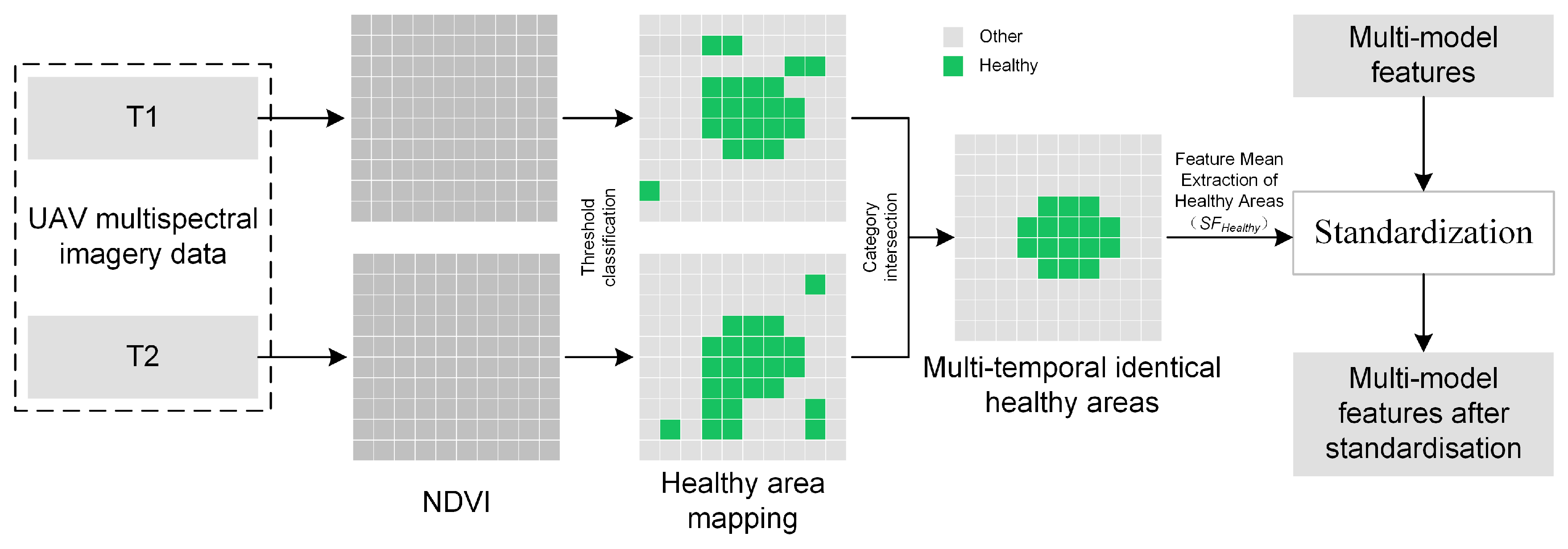
To construct a multimodal, cross-temporal generalizable monitoring model and mitigate the impact of inter-date differences on model stability, it is essential to perform the relative-difference standardization of features. In practical remote sensing data acquisition, factors such as weather conditions, solar elevation angle, and sensor operating status introduce systematic biases that weaken the comparability of data from different dates and compromise the reliability of subsequent analyses [24]. Accordingly, this study introduced a relative-difference standardization approach that selected healthy regions based on NDVI as the reference (Figure 3).

NDVI is highly sensitive to vegetation photosynthetic activity and chlorophyll content and can effectively characterize plant growth status [53]. In regions with a single disease category and low spatial heterogeneity, NDVI typically exhibits an approximately unimodal distribution, which is commonly assumed to be normal when setting thresholds [54,55]. Following this assumption, a “mean ± k × standard deviation” approach was applied, where pixels with NDVI within [μ + 0.5σ, μ + 2σ] were considered healthy vegetation. The lower (k = 0.5) and upper (k = 2) limits were selected based on preliminary experiments and on-site evaluation by tea cultivation experts. This approach effectively excludes low NDVI pixels potentially affected by stress or background interference, while the upper limit mitigates the influence of anomalously high values. After performing spatial intersection operations on the healthy regions selected for each phase, the common area identified as healthy across all phases is designated as the unified reference area. Subsequently, any multimodal feature SF is standardized using Equation (8):

$${SF}^{\prime }={\displaystyle \frac{SF-{SF}_{Healthy}}{{SF}_{Healthy}}}$$

(8)

where SF_Healthy is the mean of features within the reference region, and SF′ is the standardized feature value. Crop disease remote sensing signals are susceptible to variations in background conditions, temporal phases, and environmental factors. This variability is particularly evident in regions with complex and dynamic backgrounds, which may compromise model stability. Since the relative differences between diseased and healthy areas are generally more consistent, converting absolute feature values into relative values can effectively reduce systematic errors induced by temporal and environmental variations. This approach has been applied and validated in previous studies [56]. Constructing indices based on relative differences is thus expected to improve model generalization, robustness, and scalability in practical crop disease monitoring.

2.4.3. Optimal Selection of UAV Multi-Source Features

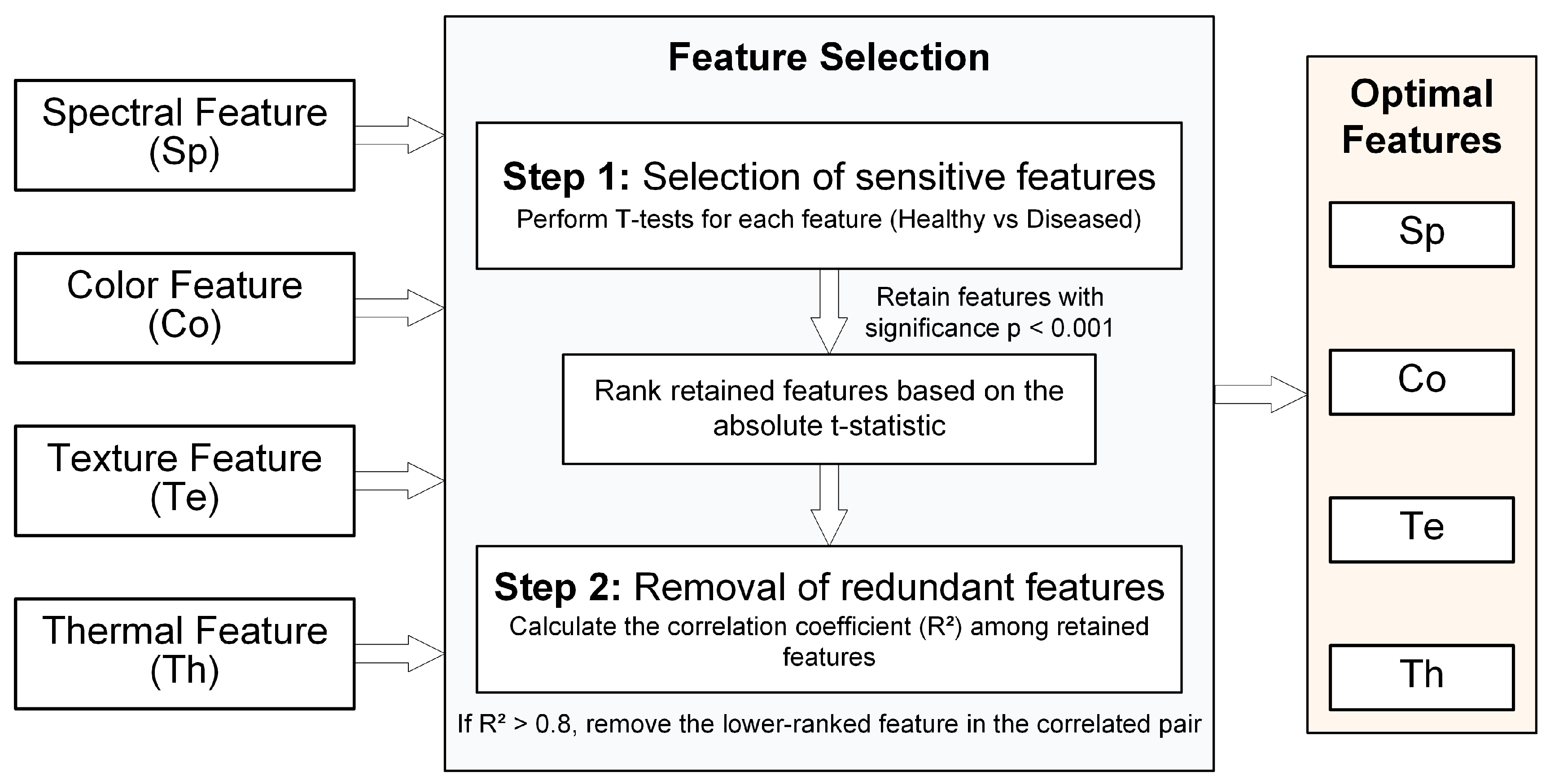
To remove redundant features, reduce feature dimensionality, and improve the model’s generalization and computational efficiency, two-step feature selection was performed for each of the four data modalities and a feature set that is sensitive to tea anthracnose was constructed (Figure 4). Firstly, we used an independent-samples t-test to examine the differences between healthy and diseased samples for each feature, and selected features showing highly significant differences between the two groups (p-value < 0.001). Then, significant features were ranked using the t-statistic (t-value), which reflects the degree of between-group difference in the t-test. Based on this, Pearson correlation coefficients were calculated for each pair of significant features. Then we eliminated the lower-ranked feature pair among those with an R² greater than 0.8. This process reduced redundancy while retaining features that exhibited more pronounced differences and offered higher independent contributions. In addition, to evaluate the performance of texture features from RGB and multispectral data in anthracnose identification, we conducted independent screening for these two feature types and selected their respective optimal combinations for subsequent analyses.

2.4.4. Construction of a Cross-Temporal General Monitoring Model for Tea Anthracnose

This study built a general monitoring model for tea anthracnose that integrated UAV multimodal data with multi-temporal information. Building upon this foundation, we evaluated the impacts of different combinations of modality features on model generalization capabilities. Multiple feature input schemes were designed: single modality (Sp, Co, Te, Th), combinations of spectral features with other modalities (Sp + Co, Sp + Te, Sp + Th), and full modality fusion (Sp + Co + Te + Th). The dataset was partitioned using stratified sampling, with 60% for calibration and 40% for validation, to ensure that both subsets were representative of the overall data in temporal distribution and the healthy/diseased ratio. This avoided distributional bias and enabled the reliable assessment of unseen data.

To reduce model complexity for practical deployment, we selected three representative machine learning algorithms: KNN, SVM, and MLP. KNN is a lazy-learning method that classifies a sample by computing its distances to the K nearest training samples in feature space and assigning the majority label. It is conceptually straightforward, simple to implement, and makes no assumptions about data distributions, making it suitable for data with pronounced local structure [57,58]. SVM seeks an optimal hyperplane that maximizes the classification margin in feature space (or in a higher-dimensional space induced by a kernel), is highly generalizable and well-suited to high-dimensional and small-sample problems, and its performance depends on the choice of kernel [59]. MLP, a typical feedforward network, learns complex relationships among inputs via nonlinear architectures with one or more hidden layers and optimizes weights by backpropagation, providing strong nonlinear modeling capacity and the ability to automatically extract high-level abstract features [60]. For each algorithm and feature combination, models were trained independently on the calibration set, and hyperparameters were optimized using grid search (GS) with five-fold cross-validation to ensure performance comparability.

Model performance was evaluated on an independent test set with four metrics (accuracy, precision, recall, and F1-score), defined as follows:

$$Accuracy={\displaystyle \frac{TP+TN}{TP+TN+FP+FN}}$$

(9)

$$Precision={\displaystyle \frac{TP}{TP+FP}}$$

(10)

$$Recall={\displaystyle \frac{TP}{TP+FN}}$$

(11)

$$F1-Score=2\times {\displaystyle \frac{Precision\times Recall}{Precision+Recall}}$$

(12)

where TP (true positive) is the number of diseased samples correctly identified, TN (true negative) is the number of healthy samples correctly identified, FP (false positive) is the number of healthy samples misclassified as diseased, and FN (false negative) is the number of diseased samples missed.

To finalize the optimal general monitoring model, we evaluated both model accuracy and multi-temporal mapping performance. First, we compared the performance of different modalities and their combinations by the highest accuracy achieved across the three algorithms for each feature input. Second, we applied the model with the highest accuracy under different modalities to multi-temporal data to classification maps and validated the mapping results against field sample points. Finally, the modality combination that showed the best performance in both model accuracy and map validation accuracy was selected. This combination was then used as the cross-temporal generalizable tea anthracnose monitoring model and tested on data from an independent temporal phase.

3. Results

3.1. Temporal Consistency Analysis of Multi-Source Features

To verify the effectiveness of the proposed relative-difference standardization in eliminating systematic bias across temporal phases, we extracted spectral data from healthy sample points and compared the distributional differences in spectral features between two phases before and after standardization (Figure 5). Healthy samples were chosen as the baseline because their vegetation status was essentially stable across temporal phases. Spectral variability mainly reflected the environmental conditions (e.g., illumination, atmosphere, minor phenological differences) or temporal differences, rather than disease stress. Accordingly, the spectral response of healthy samples served as an ideal reference for assessing bias introduced by temporal differences.

Figure 5a indicates that without standardization, there were significant differences in the Green, RedEdge, and NIR bands between healthy samples at the two phases, while only the Red band was relatively stable. This suggests that the Green, RedEdge, and NIR bands were highly sensitive to temporal phases even for the same healthy condition, prone to pronounced shifts across phases that confound detection of anthracnose-induced spectral changes in tea and weaken model robustness and cross-temporal generalization.

In contrast, Figure 5b shows that after relative-difference standardization, there were no significant band differences across phases for healthy samples, and the data distributions were highly consistent. This demonstrates that the standardized method of selecting healthy areas based on NDVI as a baseline effectively eliminated feature shifts caused by temporal differences, providing a unified basis for feature representation across phases and thereby improving disease identification accuracy and cross-temporal generalization. In summary, this standardization procedure laid the groundwork for consistent comparison and modeling of diseased samples across temporal phases.

The study also selected healthy samples from different phases for comparison to validate the superiority of the proposed VSRT temperature feature over the commonly used NRCT in cross-temporal consistency (Figure 6). The results showed that NRCT exhibited significant differences between the two datasets acquired at different times. Consequently, training cross-temporal models using this feature introduced substantial errors, hindering model generalization. In contrast, VSRT showed no significant differences between the two datasets acquired at different times, maintaining excellent consistency. This provided a robust temperature representation for constructing cross-temporal general monitoring models by integrating thermal infrared features.

3.2. Optimal Selection of a Multi-Source Sensitive Feature Set for Tea Anthracnose

This study extracted four types of modal features (spectral, thermal, texture, and color) based on UAV multispectral, thermal infrared, and RGB imagery. To build an effective feature set for tea anthracnose, we first conducted a sensitivity analysis of spectral, texture and color features (t-tests between healthy and diseased samples, p-value < 0.001) and removed features that were insensitive to tea anthracnose. Furthermore, correlation analysis was conducted on the selected sensitive features to reduce redundancy, and the correlation coefficient matrix is shown in Figure 7. Of the spectral features, vegetation indices with higher sensitivity rankings, such as SR, MSR, DVIRE, WDRVI, and CIG, exhibited strong collinearity. By removing the lower-ranked feature from each highly correlated pair, we ultimately retained seven spectral features with greater distinctiveness and stronger complementarity (

Table 5. The final selection results of different kinds of features.

Feature Type	Feature Name
Sp	SR, NIR, NormRRE, VARIG, Red, RedEdge, ARI
Te	NIR_D[MEA,HOM], NIR_R[SEC,MEA], RedEdge_N[MEA,SEC], Gray_R[MEA,DIS], Gray_D[MEA,DIS], Gray_N[VAR,DIS]
Co	ExR, R, ExG, B
Th	VSRT

Note: Sp represents spectral features, Te represents texture features, Co represents color features, Th represents thermal features.

). Of these, SR effectively suppressed non-vegetation background interference and characterized plant growth traits [61]. ARI and VARIG were highly sensitive to changes in critical pigments (e.g., anthocyanins, chlorophyll) and could directly indicate pigment degradation caused by disease [39,62]. Meanwhile, the standardized original NIR, Red, and RedEdge bands, used as base variables, responded directly to cellular structural scattering, pigment absorption, and internal leaf structural changes [63]. This provided a direct and complementary spectral basis for disease-induced physiological and biochemical changes.

For color indices computed from RGB, distinct correlation clusters likewise existed (e.g., ExG, NGRDI, MGRVI, and GLI all emphasized “greenness” information). After redundancy removal, the four most representative color features were ultimately retained (Table 5). Of them, ExG was sensitive to leaf chlorosis or loss of greenness and was closely related to foliar disease [64]. ExR was correlated with multiple vegetation growth parameters (e.g., nitrogen content, chlorophyll) [65]. Additionally, the normalized R and B original color components preserved spectral information in the visible region, which was important for capturing spectral responses of different pigments (e.g., chlorophyll absorbs red and blue light, carotenoids absorb blue light) [66].

In evaluating texture features, the study retained the three optimal texture-feature combinations from spectral and RGB-gray data sources. The final set of spectral texture features included NIR_D[MEA,HOM], NIR_R[SEC,MEA], and RedEdge_N[MEA,SEC]. The NIR and RedEdge bands were the most sensitive to vegetation status. MEA (mean) reflected overall texture brightness variations caused by lesions, whereas SEC (second-order moment) characterized lesion-internal or edge roughness and contrast [17,67]. For RGB-gray texture features, the final selection retained Gray_R[MEA,DIS], Gray_D[MEA,DIS], and Gray_N[VAR,DIS], where DIS (dissimilarity) measured the frequency of dissimilar pixel pairs in the co-occurrence matrix and responded to abrupt boundaries and heterogeneous regions between lesions and healthy tissue [17,67].

Of the temperature features, VSRT outperformed NRCT in cross-temporal consistency while exhibiting higher sensitivity to disease. This made it the optimal temperature feature selected.

In summary, dual screening via sensitivity testing and correlation analysis was used to obtain a set of sensitive features with significant discriminability and strong complementarity across modalities. This feature set reflected the impacts of tea anthracnose on leaf and canopy status, from spectral, color, texture, and temperature perspectives, laying a solid foundation for constructing accurate and robust monitoring models.

3.3. Comparison of Models That Combine Multi-Source Features with Different Algorithms

This study compared models for monitoring tea anthracnose constructed from various multimodal feature combinations, with results shown in

Table 6. Evaluation results of the model based on different feature combinations and algorithms.

Feature Type	Metrics	KNN	SVM	MLP
Sp	Accuracy	89.10%	93.59%	90.38%
	Precision	89.30%	93.64%	90.40%
	Recall	89.01%	93.55%	90.36%
	F1-Score	89.07%	93.58%	90.37%
Te	Accuracy	89.74%	90.38%	93.59%
	Precision	89.74%	90.41%	93.59%
	Recall	89.77%	90.43%	93.59%
	F1-Score	89.74%	90.38%	93.59%
Co	Accuracy	85.90%	85.90%	85.26%
	Precision	85.90%	85.90%	85.32%
	Recall	85.92%	85.92%	85.20%
	F1-Score	85.90%	85.90%	85.23%
Th	Accuracy	64.10%	67.95%	68.59%
	Precision	64.21%	71.64%	69.56%
	Recall	64.18%	68.45%	68.85%
	F1-Score	64.10%	66.88%	68.37%
Sp + Te	Accuracy	93.59%	91.67%	85.90%
	Precision	93.59%	91.68%	85.95%
	Recall	93.59%	91.64%	85.95%
	F1-Score	93.59%	91.66%	85.90%
Sp + Co	Accuracy	94.23%	92.95%	89.74%
	Precision	94.33%	92.96%	89.80%
	Recall	94.18%	92.93%	89.80%
	F1-Score	94.22%	92.94%	89.74%
Sp + Th	Accuracy	95.51%	94.23%	92.95%
	Precision	95.53%	94.33%	92.97%
	Recall	95.49%	94.18%	92.99%
	F1-Score	95.51%	94.22%	92.95%
Sp + Te + Co + Th	Accuracy	92.95%	90.38%	92.95%
	Precision	93.04%	90.41%	92.96%
	Recall	92.89%	90.43%	92.93%
	F1-Score	92.93%	90.38%	92.94%

Note: Sp represents spectral features, Te represents texture features, Co represents color features, Th represents thermal features. Bold indicates the highest accuracy value among the three algorithms.

. Under single-modality features, Sp and Te performed markedly better than Co and Th. In particular, the highest classification accuracy for both Sp and Te was 93.59%. In comparison, Co and Th attained respective peak accuracies of 85.90% and 68.59%, which were substantially inferior to the Sp and Te modalities. The superior performance of Sp likely stemmed from its ability to directly characterize leaf biochemical and microstructural changes induced by disease, whereas Co, Te, and Th mostly had indirect or lagged responses. Te, which leveraged both spectral and RGB data, also stood out in the single-modality comparison.

Introducing other modalities on top of Sp further improved the overall model accuracy. In particular, “Sp + Th” achieved a maximum accuracy of 95.51%, improving upon the best single-modality accuracies of Sp, Th, Te, and Co by approximately 2%, 27%, 2%, and 10%, respectively. This indicates that although Th alone performed poorly, when combined with Sp it provided complementary information that markedly enhanced the model’s discriminative capability.

Algorithmically, SVM and MLP performed well under single-modality performance with maximum accuracies of 93.59%. In contrast, KNN achieved a maximum of 89.74%. However, after multimodal feature fusion, KNN exhibited the most pronounced improvement, reaching 95.51% with the “Sp + Th” combination and outperforming SVM (94.23%) and MLP (92.95%). These results implied that KNN was better able to exploit complementary information among modalities in a high-dimensional feature space. Regarding classification metrics, the KNN algorithm exhibited the highest precision (95.53%) and recall (95.49%), reflecting a well-balanced performance. Analyzing the confusion matrices of the three algorithms under the “Sp + Th” feature combination (

Table 7. Confusion matrix–based performance of three algorithms under the “Sp + Th” combination.

Model	TN	FP	FN	TP	Accuracy	Precision	Recall	F1-Score
KNN	72	4	3	77	95.51%	95.53%	95.49%	95.51%
SVM	70	6	3	77	94.23%	94.33%	94.18%	94.22%
MLP	72	4	7	73	92.95%	92.97%	92.99%	92.95%

Note: Precision, Recall, and F1-score are reported as macro-averages computed across the two classes (Healthy and Diseased).

), it was observed that SVM demonstrated a greater tendency to produce false positives, misclassifying six healthy instances as diseased, compared to four misclassifications for both KNN and MLP. In contrast, MLP showed a higher number of false negatives, failing to identify seven diseased instances, whereas KNN and SVM missed only three.

Overall, “Sp + Th” was the optimal modality combination for tea anthracnose monitoring. Coupled with the simple and efficient KNN algorithm, it delivered the highest accuracy and cross-temporal stability, laying the groundwork for robust operational deployment.

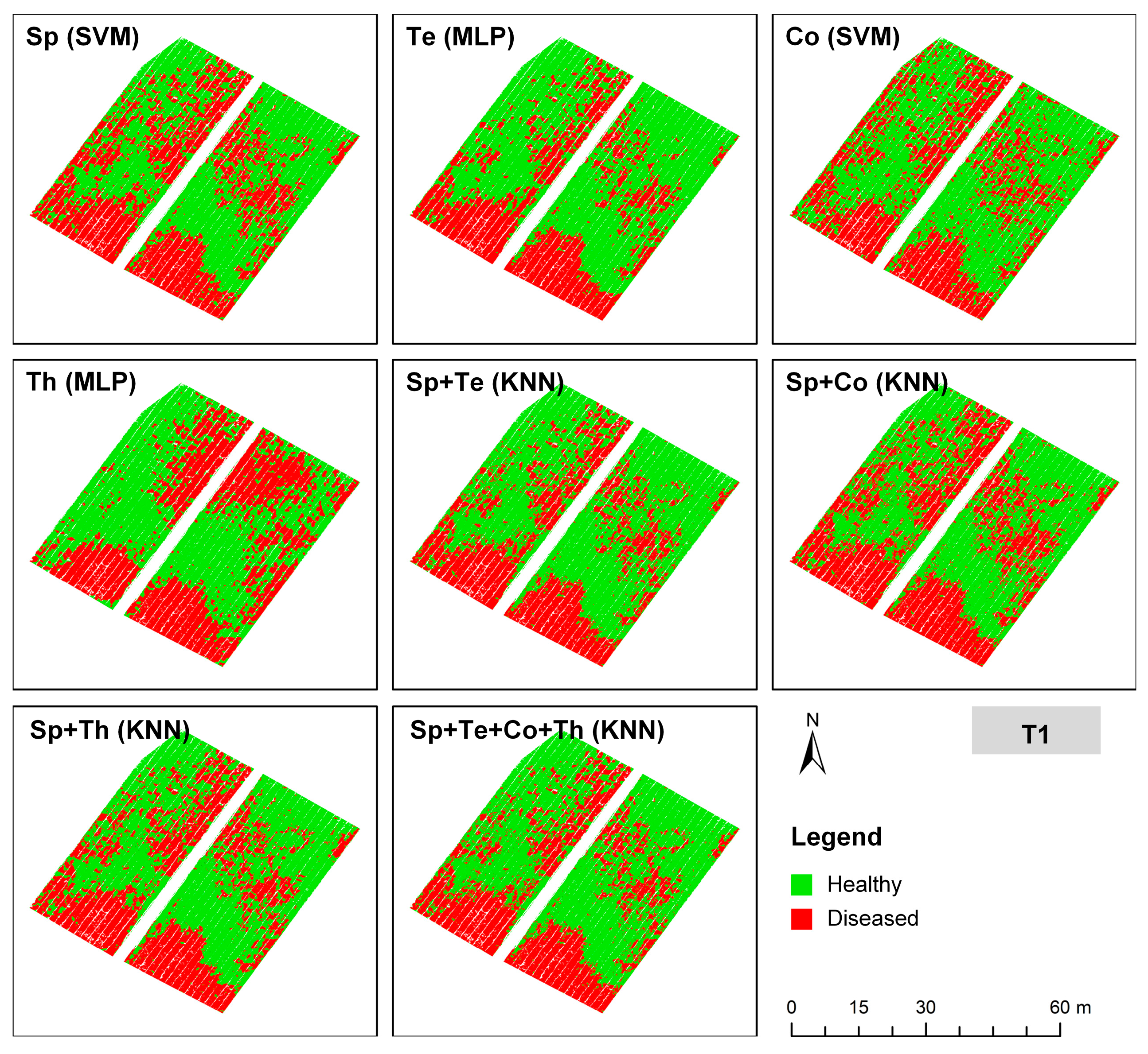
We next conducted classification mapping of tea anthracnose for two temporal phases using the best model under each modality to further evaluate the spatiotemporal practicality of the models (Figure 8 and Figure 9). The results showed that mapping derived from Sp, alone or fused with other modalities consistently captured the spatial distribution of disease, with concentrated infection in the field’s southwest and scattered infection in the central region. By contrast, when Te, Th, or Co were used alone, the maps exhibited local omissions or substantial noise. Moreover, the Th and Co modalities differed markedly between the two temporal phases, whereas the Te modality was more consistent but lacked a detailed depiction of disease.

Validation at ground survey points (

Table 8. The accuracy of mapping results under different feature combinations based on sample points.

Feature Type	T1 Val. Acc.	T2 Val. Acc.	Mean Val. Acc. (T1, T2)
Sp	100.00%	98.04%	99.02%
Te	100.00%	96.08%	98.04%
Co	89.13%	86.27%	87.70%
Th	89.13%	58.82%	73.98%
Sp + Te	97.83%	96.08%	96.96%
Sp + Co	97.83%	100.00%	98.92%
Sp + Th	100.00%	100.00%	100.00%
Sp + Te + Co + Th	97.83%	100.00%	98.92%

Note: Sp represents spectral features, Te represents texture features, Co represents color features, Th represents thermal features; Val. Acc.: validation accuracy; Mean Val. Acc. (T1–T2) is computed as (T1 Val. Acc. + T2 Val. Acc.)/2.

) further corroborated these findings: under a single modality, Sp yielded the highest average mapping accuracy (99.02%), followed by Te at 98.04%. Under multimodal fusion, the “Sp + Th” combination achieved the highest accuracy, reaching 100.00% at both temporal phases and clearly surpassing all other combinations. In contrast, fusing all modalities (Sp + Te + Co + Th) produced slightly lower accuracy (98.92%), which was likely due to information redundancy or mild overfitting. It is worth noting that the single Te modality differed greatly between the two temporal phases (by 30.31%), but when combined with Sp, the accuracy improved substantially and exhibited cross-temporal stability.

Finally, the differences between mapping results generated from three inputs, single: Sp; Sp + Th; and all modalities (Figure 10), were analyzed. Because the interval between the two temporal phases was short and overall disease progression within the field was limited, the maps were largely consistent. Specifically, the Healthy-to-Diseased (HD) and Diseased-to-Healthy (DH) categories accounted for a small proportion of the total and were mainly located along the edges of disease-concentrated areas. HD occurred mostly within infected zones, reflecting ongoing disease development, whereas DH appeared more at the edges, reflecting minor classification differences between phases. Among these, classification differences may partly stem from errors caused by data noise or mixed pixels, as well as misclassification due to the similarity of features between healthy and mildly diseased pixels. Additionally, due to plant growth or disease progression, the edges between healthy and diseased areas are often the most dynamic, where classification results may be affected by edge effects, leading to discontinuities or errors in these regions. Overall, the “Sp + Th” fusion model not only exhibited high stability across time phases but also revealed the trends of disease progression to some extent.

To further demonstrate the generalizability of the model based on the optimal feature combination (“Sp + Th”) and algorithm (KNN) in practical applications, the study used independent T3 temporal data for mapping validation (Figure 11). The validation accuracy, based on actual survey points from the T3 temporal data, was 86.41%. As shown in the figure, after a one-year time span, the upper half of the plot showed a more concentrated distribution of disease, while the lower half had a more dispersed distribution. Although there were some misclassifications in the more dispersed disease areas, the model was able to accurately assess the overall disease occurrence. These results indicate that the tea anthracnose monitoring model, constructed with the “Sp + Th” combination and KNN algorithm for multi-temporal data, exhibits high generalizability and temporal-phase robustness.

4. Discussion

This study proposed a relative-difference standardization method based on NDVI to improve the feature consistency of UAV remote sensing data across different acquisition times. Specifically, at each observation time, NDVI was used to select relatively healthy vegetation areas as the reference, and multimodal features were normalized accordingly. This effectively mitigated the systematic shifts caused by illumination conditions, sensor status, or differences in plant physiological stage. Previous studies on change detection and image classification using multi-temporal imagery have employed relative radiometric normalization techniques. Common approaches include the use of a reference image or the matching of pseudo-invariant features (PIF) [68,69]. However, under field environments with complicated crop growing status, identifying invariant areas for PIF extraction becomes relatively difficult. Although some studies have suggested optimizing PIF feature processing using weakly supervised GAN models [70], such approaches typically require complex model-building processes. Additionally, this normalization approach also lacks validation on UAV imagery data. Different from previous studies, the cross-temporal standardization method proposed in this study offers a more straightforward and applicable solution for UAV remotely sensed monitoring. From a mechanistic perspective, the spectral responses of healthy samples remained relatively stable across different phases. This stability allows them to serve as a reliable reference for correcting spectral variations caused by non-disease factors [24]. This strategy was significant for two main reasons: first, it enhanced the model’s sensitivity to disease traits, more accurately characterizing disease-induced spectral and thermal changes while suppressing external disturbances. Second, it improved generalization across times and observational conditions, providing a solid data foundation for cross-temporal disease recognition and dynamic monitoring [20,71].

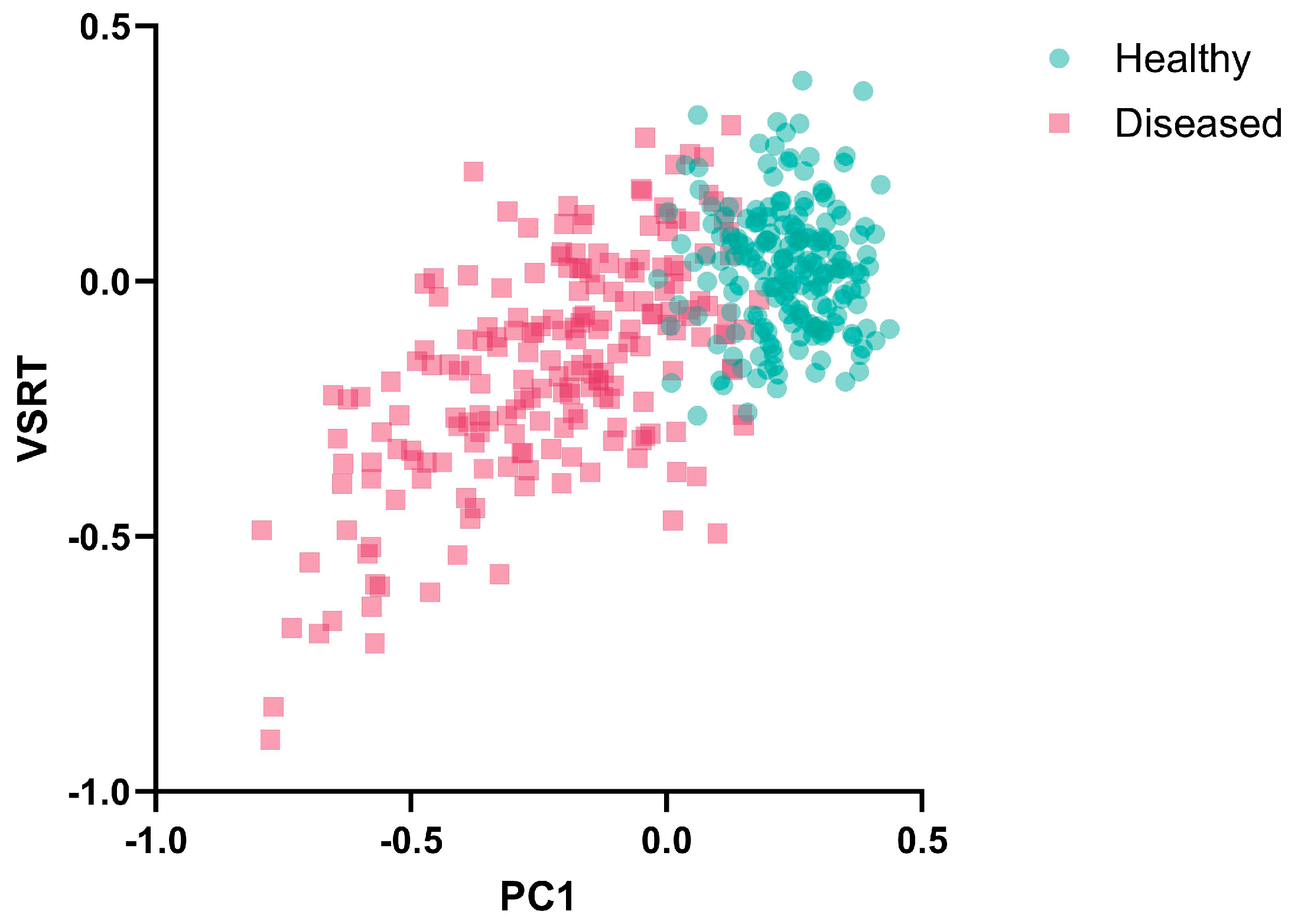
When creating the cross-temporal model, this study compared multiple modality combinations and found that combining spectral and thermal features markedly improved model accuracy and stability. Previous studies have also shown that combining spectral and temperature can simultaneously characterize changes in vegetation physiological status and stomatal conductance. This approach has been validated as reliable for monitoring stresses such as drought, diseases, and water deficits [9,18,72,73]. To explore the underlying mechanism, we visualized healthy and diseased samples in the joint spectral–thermal feature space (Figure 12). Specifically, the spectral dimension used PCA to extract the first principal component (PC1), retaining 95% of the variance. The thermal dimension adopted the VSRT. The results showed that the two classes were clearly separated in the two-dimensional PC1–VSRT space. This was likely due to anthracnose infection in tea leaves, which altered the concentrations of physiological and biochemical constituents, resulting in canopy spectral changes (decreased PC1). At the same time, changes in transpiration and water status led to shifts in canopy temperature (decreased VSRT). These two effects were complementary, making diseased samples easier to distinguish in feature space. Additionally, to enhance the temporal stability of temperature-based features, this study introduced the Vegetation–Soil Relative Temperature (VSRT) index. This index quantifies the temperature contrast between vegetation canopies and adjacent bare soil, and its consistency across multiple observation phases was verified. It should be noted, however, that VSRT stability may be influenced by several environmental factors. Variations in soil moisture and texture can alter soil evaporation rates, water-holding capacity, and thermal inertia, thereby affecting the magnitude and diurnal dynamics of soil surface temperature [74]. Likewise, local microclimate conditions and canopy density can regulate convective heat exchange and energy balance within the canopy, indirectly influencing canopy temperature [75]. Although this study was conducted within a relatively homogeneous area where such effects were minimized, further systematic validation under diverse environmental settings is warranted to confirm the robustness of VSRT.

This study compared multiple machine learning algorithms under different modality combinations. The results indicated that under single-modality conditions, SVM and MLP outperformed KNN, whereas KNN demonstrated the best performance in multimodal fusion scenarios. As a distance-based non-parametric instance learning method, KNN is prone to performance instability in single-modality situations, influenced by the challenges posed by high-dimensional spaces, noise, and local imbalances [76]. However, within the fused or expanded feature space, the neighborhood structure becomes more pronounced. Research in various applications, such as multi-sensor human activity recognition and multimodal EEG-based depression recognition, has shown that KNN performs well in modality fusion situations [77,78]. Similarly, in plant disease identification, KNN outperformed SVM when using deep network-extracted embeddings, with KNN’s neighborhood voting proving more effective in thoroughly represented feature spaces [79]. Consistent with these findings, the confusion matrix results in this study showed that SVM had a higher number of false positives (healthy samples misclassified as diseased), while MLP exhibited more false negatives (Table 7). In contrast, KNN achieved a more balanced classification, effectively reducing both types of errors. This balance renders KNN particularly advantageous for cross-temporal monitoring tasks in this study. Furthermore, compared to end-to-end deep fusion models, KNN requires no complex training and is highly cost-effective. This makes it well-suited for small-to-medium-sized datasets and rapid engineering deployment.

The cross-temporal general monitoring framework proposed in this study demonstrated robust stability and strong generalization capabilities. Operating at the tea plantation scale through multimodal fusion and relative-difference standardization, it proved effective for monitoring anthracnose across time. Compared to other methods that rely on single-phase images, this framework maintained stable prediction performance under varying acquisition conditions, demonstrating strong robustness to cross-temporal variability. Moreover, by utilizing an industry-grade UAV platform and a simplified modeling workflow, this approach reduced dependence on equipment and data acquisition conditions while maintaining accuracy. This, in turn, enhanced repeatability across diverse regions and temporal phases. It should be noted that this study was primarily conducted in tea gardens with relatively uniform cultivars, with anthracnose as the primary focus. Although the results validated the effectiveness of the method, its applicability in more complex crop systems, multi-stress situations, and conditions with imbalanced sample distributions requires further investigation. Future work will focus on three aspects: (1) verifying the method’s generality in other pest and stress contexts (e.g., tea green leafhopper, geometrid caterpillars, and heat stress); (2) introducing self-supervised learning, multi-task learning, and spatiotemporal attention mechanisms to enhance model representation and generalization under complex targets and imbalanced samples [80,81]; and (3) coupling meteorological and plant-protection monitoring data in space and time, and integrating crop process mechanisms with outcome uncertainty assessment to improve the credibility and interpretability of regional early warning [82,83,84].

5. Conclusions

This study proposed a cross-temporal general monitoring method for the precise and efficient surveillance of tea anthracnose disease, based on UAV multimodal fusion combined with relative-difference standardization. The main conclusions are as follows:

(1)

A relative-difference standardization strategy that uses NDVI identified healthy regions as the reference was proposed and validated, which effectively addressed feature inconsistencies among remote sensing data acquired at different times. Meanwhile, we constructed the innovative VSRT index, which exhibited higher temporal consistency and robustness compared to the Normalized Relative Canopy Temperature (NRCT).

(2)

A multimodal feature set was constructed using seven spectral features (SR, NIR, NormRRE, VARI_Green, Red, RedEdge, ARI), six texture features (NIR_D[MEA,HOM], NIR_R[SEC,MEA], RedEdge_N[MEA,SEC], Gray_R[MEA,DIS], Gray_D[MEA,DIS], Gray_N[VAR,DIS]), four color features (ExR, R, ExG, B), and one thermal feature (VSRT).

(3)

Among all model configurations, the multimodal combination of spectral and thermal features (‘Sp + Th’) integrated with the K-Nearest Neighbor (KNN) algorithm achieved the highest classification accuracy of 95.51%, confirming its superior capability for tea anthracnose detection and generalization.

In conclusion, the proposed method can enable accurate cross-temporal monitoring of tea anthracnose and is robust and effective under varying temporal conditions. The relative-difference standardization strategy employed in this study demonstrated advantages in reducing dependence on equipment and acquisition conditions and providing a viable approach for dynamic monitoring and rapid diagnosis of multiple crop diseases. Future research will expand the proposed framework to tea fields with different cultivars and soil types to validate its adaptability under diverse agroecological conditions. In addition, we plan to integrate NDVI-based standardization with existing agricultural monitoring systems and explore lightweight, attention-based AI models to enhance computational efficiency and cross-domain scalability. These efforts will contribute to building a more intelligent, generalizable, and operational monitoring system for tea and other crop diseases.

References

1. Orrock, J.M.; Rathinasabapathi, B.; Spakes Richter, B. Anthracnose in U.S. Tea: Pathogen Characterization and Susceptibility Among Six Tea Accessions. Plant Dis. 2020, 104, 1055–1059. [Google Scholar] [CrossRef]
2. Chen, M.; Zhong, L.; Zhang, Z.; Peng, C.; Ke, D.; Gan, P.; Wang, Z.; Wei, R.; Liu, W.; Yang, J. Isolation and Identification of Colletotrichum as Fungal Pathogen from Tea and Preliminary Fungicide Screening. Qual. Assur. Saf. Crops Foods 2022, 14, 92–101. [Google Scholar] [CrossRef]
3. He, S.; Chen, H.; Wei, Y.; An, T.; Liu, S. Development of a DNA-Based Real-Time PCR Assay for the Quantification of Colletotrichum Camelliae Growth in Tea (Camellia sinensis). Plant Methods 2020, 16, 17. [Google Scholar] [CrossRef] [PubMed]
4. Pandey, A.K.; Sinniah, G.D.; Babu, A.; Tanti, A. How the Global Tea Industry Copes with Fungal Diseases—Challenges and Opportunities. Plant Dis. 2021, 105, 1868–1879. [Google Scholar] [CrossRef]
5. Bao, W.; Zhu, Z.; Hu, G.; Zhou, X.; Zhang, D.; Yang, X. UAV Remote Sensing Detection of Tea Leaf Blight Based on DDMA-YOLO. Comput. Electron. Agric. 2023, 205, 107637. [Google Scholar] [CrossRef]
6. Phang, S.K.; Chiang, T.H.A.; Happonen, A.; Chang, M.M.L. From Satellite to UAV-Based Remote Sensing: A Review on Precision Agriculture. IEEE Access 2023, 11, 127057–127076. [Google Scholar] [CrossRef]
7. Alvarez-Vanhard, E.; Corpetti, T.; Houet, T. UAV & Satellite Synergies for Optical Remote Sensing Applications: A Literature Review. Sci. Remote Sens. 2021, 3, 100019. [Google Scholar] [CrossRef]
8. Li, W.; He, J.; Yu, M.; Su, X.; Wang, X.; Zheng, H.; Yao, X.; Cheng, T.; Zhu, Y.; Cao, W.; et al. Multisource Remote Sensing Data-Driven Estimation of Rice Grain Starch Accumulation: Leveraging Matter Accumulation and Translocation Characteristics. IEEE Trans. Geosci. Remote Sens. 2024, 62, 4416818. [Google Scholar] [CrossRef]
9. Chakhvashvili, E.; Machwitz, M.; Antala, M.; Rozenstein, O.; Prikaziuk, E.; Schlerf, M.; Naethe, P.; Wan, Q.; Komárek, J.; Klouek, T.; et al. Crop Stress Detection from UAVs: Best Practices and Lessons Learned for Exploiting Sensor Synergies. Precis. Agric. 2024, 25, 2614–2642. [Google Scholar] [CrossRef]
10. Bhandari, M.; Ibrahim, A.M.H.; Xue, Q.; Jung, J.; Chang, A.; Rudd, J.C.; Maeda, M.; Rajan, N.; Neely, H.; Landivar, J. Assessing Winter Wheat Foliage Disease Severity Using Aerial Imagery Acquired from Small Unmanned Aerial Vehicle (UAV). Comput. Electron. Agric. 2020, 176, 105665. [Google Scholar] [CrossRef]
11. Su, J.; Liu, C.; Coombes, M.; Hu, X.; Wang, C.; Xu, X.; Li, Q.; Guo, L.; Chen, W. Wheat Yellow Rust Monitoring by Learning from Multispectral UAV Aerial Imagery. Comput. Electron. Agric. 2018, 155, 157–166. [Google Scholar] [CrossRef]
12. Abdulridha, J.; Ampatzidis, Y.; Kakarla, S.C.; Roberts, P. Detection of Target Spot and Bacterial Spot Diseases in Tomato Using UAV-Based and Benchtop-Based Hyperspectral Imaging Techniques. Precis. Agric. 2020, 21, 955–978. [Google Scholar] [CrossRef]
13. Xu, D.; Lu, Y.; Liang, H.; Lu, Z.; Yu, L.; Liu, Q. Areca Yellow Leaf Disease Severity Monitoring Using UAV-Based Multispectral and Thermal Infrared Imagery. Remote Sens. 2023, 15, 3114. [Google Scholar] [CrossRef]
14. Jiang, J.; Ji, H.; Zhou, G.; Pan, R.; Zhao, L.; Duan, Z.; Liu, X.; Yin, J.; Duan, Y.; Ma, Y.; et al. Non-Destructive Monitoring of Tea Plant Growth through UAV Spectral Imagery and Meteorological Data Using Machine Learning and Parameter Optimization Algorithms. Comput. Electron. Agric. 2025, 229, 109795. [Google Scholar] [CrossRef]
15. Sahoo, M.M.; Tarshish, R.; Tubul, Y.; Sabag, I.; Gadri, Y.; Morota, G.; Peleg, Z.; Alchanatis, V.; Herrmann, I. Multimodal Ensemble of UAV-Borne Hyperspectral, Thermal, and RGB Imagery to Identify Combined Nitrogen and Water Deficiencies in Field-Grown Sesame. ISPRS J. Photogramm. Remote Sens. 2025, 222, 33–53. [Google Scholar] [CrossRef]
16. Zhu, X.; Liu, X.; Wu, Q.; Liu, M.; Hu, X.; Deng, H.; Zhang, Y.; Qu, Y.; Wang, B.; Gou, X.; et al. Utilizing UAV-Based High-Throughput Phenotyping and Machine Learning to Evaluate Drought Resistance in Wheat Germplasm. Comput. Electron. Agric. 2025, 237, 110602. [Google Scholar] [CrossRef]
17. Ma, R.; Zhang, N.; Zhang, X.; Bai, T.; Yuan, X.; Bao, H.; He, D.; Sun, W.; He, Y. Cotton Verticillium Wilt Monitoring Based on UAV Multispectral-Visible Multi-Source Feature Fusion. Comput. Electron. Agric. 2024, 217, 108628. [Google Scholar] [CrossRef]
18. Liu, Y.; Liu, G.; Sun, H.; An, L.; Zhao, R.; Liu, M.; Tang, W.; Li, M.; Yan, X.; Ma, Y.; et al. Exploring Multi-Features in UAV Based Optical and Thermal Infrared Images to Estimate Disease Severity of Wheat Powdery Mildew. Comput. Electron. Agric. 2024, 225, 109285. [Google Scholar] [CrossRef]
19. Liu, T.; Qi, Y.; Yang, F.; Yi, X.; Guo, S.; Wu, P.; Yuan, Q.; Xu, T. Early Detection of Rice Blast Using UAV Hyperspectral Imagery and Multi-Scale Integrator Selection Attention Transformer Network (MS-STNet). Comput. Electron. Agric. 2025, 231, 110007. [Google Scholar] [CrossRef]
20. Wang, Y.; Yang, Z.; Khan, H.A.; Kootstra, G. Improving Radiometric Block Adjustment for UAV Multispectral Imagery under Variable Illumination Conditions. Remote Sens. 2024, 16, 3019. [Google Scholar] [CrossRef]
21. Wang, Z.; Zhou, J.; Ma, J.; Wang, Y.; Liu, S.; Ding, L.; Tang, W.; Pakezhamu, N.; Meng, L. Removing Temperature Drift and Temporal Variation in Thermal Infrared Images of a UAV Uncooled Thermal Infrared Imager. ISPRS J. Photogramm. Remote Sens. 2023, 203, 392–411. [Google Scholar] [CrossRef]
22. Messina, G.; Modica, G. Applications of UAV Thermal Imagery in Precision Agriculture: State of the Art and Future Research Outlook. Remote Sens. 2020, 12, 1491. [Google Scholar] [CrossRef]
23. Uddin, S.; Lu, H. Dataset Meta-Level and Statistical Features Affect Machine Learning Performance. Sci. Rep. 2024, 14, 1670. [Google Scholar] [CrossRef]
24. Schott, J.R.; Salvaggio, C.; Volchok, W.J. Radiometric Scene Normalization Using Pseudoinvariant Features. Remote Sens. Environ. 1988, 26, 1–14. [Google Scholar] [CrossRef]
25. Zhu, H.; Lin, C.; Liu, G.; Wang, D.; Qin, S.; Li, A.; Xu, J.-L.; He, Y. Intelligent Agriculture: Deep Learning in UAV-Based Remote Sensing Imagery for Crop Diseases and Pests Detection. Front. Plant Sci. 2024, 15, 1435016. [Google Scholar] [CrossRef]
26. Ochiai, S.; Kamada, E.; Sugiura, R. Comparative Analysis of RGB and Multispectral UAV Image Data for Leaf Area Index Estimation of Sweet Potato. Smart Agric. Technol. 2024, 9, 100579. [Google Scholar] [CrossRef]
27. Wang, X.; Yan, S.; Wang, W.; Yin, L.; Li, M.; Yu, Z.; Chang, S.; Hou, F. Monitoring Leaf Area Index of the Sown Mixture Pasture through UAV Multispectral Image and Texture Characteristics. Comput. Electron. Agric. 2023, 214, 108333. [Google Scholar] [CrossRef]
28. Sun, H.; Song, X.; Guo, W.; Guo, M.; Mao, Y.; Yang, G.; Feng, H.; Zhang, J.; Feng, Z.; Wang, J.; et al. Potato Late Blight Severity Monitoring Based on the Relief-mRmR Algorithm with Dual-Drone Cooperation. Comput. Electron. Agric. 2023, 215, 108438. [Google Scholar] [CrossRef]
29. Elsayed, S.; Rischbeck, P.; Schmidhalter, U. Comparing the Performance of Active and Passive Reflectance Sensors to Assess the Normalized Relative Canopy Temperature and Grain Yield of Drought-Stressed Barley Cultivars. Field Crops Res. 2015, 177, 148–160. [Google Scholar] [CrossRef]
30. Gitelson, A.A. Wide Dynamic Range Vegetation Index for Remote Quantification of Biophysical Characteristics of Vegetation. J. Plant Physiol. 2004, 161, 165–173. [Google Scholar] [CrossRef] [PubMed]
31. Gitelson, A.A.; Kaufman, Y.J.; Stark, R.; Rundquist, D. Novel Algorithms for Remote Estimation of Vegetation Fraction. Remote Sens. Environ. 2002, 80, 76–87. [Google Scholar] [CrossRef]
32. Jordan, C.F. Derivation of Leaf-Area Index from Quality of Light on the Forest Floor. Ecology 1969, 50, 663–666. [Google Scholar] [CrossRef]
33. Huete, A.R. A Soil-Adjusted Vegetation Index (SAVI). Remote Sens. Environ. 1988, 25, 295–309. [Google Scholar] [CrossRef]
34. Jiang, Z.; Huete, A.R.; Didan, K.; Miura, T. Development of a Two-Band Enhanced Vegetation Index without a Blue Band. Remote Sens. Environ. 2008, 112, 3833–3845. [Google Scholar] [CrossRef]
35. Rouse, J.W., Jr.; Haas, R.H.; Schell, J.A.; Deering, D.W. Monitoring Vegetation Systems in the Great Plains with Erts. NASA Spec. Publ. 1974, 351, 309. [Google Scholar]
36. Gitelson, A.; Merzlyak, M.N. Quantitative Estimation of Chlorophyll-a Using Reflectance Spectra: Experiments with Autumn Chestnut and Maple Leaves. J. Photochem. Photobiol. B 1994, 22, 247–252. [Google Scholar] [CrossRef]
37. Gitelson, A.A.; Viña, A.; Arkebauer, T.J.; Rundquist, D.C.; Keydan, G.; Leavitt, B. Remote Estimation of Leaf Area Index and Green Leaf Biomass in Maize Canopies. Geophys. Res. Lett. 2003, 30, 1248. [Google Scholar] [CrossRef]
38. Kim, M.S.; Daughtry, C.S.T.; Chappelle, E.W.; Mcmurtrey, J.E.; Walthall, C.L. The Use of High Spectral Resolution Bands for Estimating Absorbed Photosynthetically Active Radiation (A Par). In Proceedings of the 6th International Symposium on Physical Measurements and Signatures in Remote Sensing, CNES, Val D’Isere, France, 17–21 January 1994. [Google Scholar]
39. Gitelson, A.A.; Merzlyak, M.N.; Chivkunova, O.B. Optical Properties and Nondestructive Estimation of Anthocyanin Content in Plant Leaves. Photochem. Photobiol. 2001, 74, 38–45. [Google Scholar] [CrossRef]
40. Roujean, J.-L.; Breon, F.-M. Estimating PAR Absorbed by Vegetation from Bidirectional Reflectance Measurements. Remote Sens. Environ. 1995, 51, 375–384. [Google Scholar] [CrossRef]
41. Gitelson, A.A.; Kaufman, Y.J.; Merzlyak, M.N. Use of a Green Channel in Remote Sensing of Global Vegetation from EOS-MODIS. Remote Sens. Environ. 1996, 58, 289–298. [Google Scholar] [CrossRef]
42. Qi, J.; Chehbouni, A.; Huete, A.R.; Kerr, Y.H.; Sorooshian, S. A Modified Soil Adjusted Vegetation Index. Remote Sens. Environ. 1994, 48, 119–126. [Google Scholar] [CrossRef]
43. Chen, J.M. Evaluation of Vegetation Indices and a Modified Simple Ratio for Boreal Applications. Can. J. Remote Sens. 1996, 22, 229–242. [Google Scholar] [CrossRef]
44. Rondeaux, G.; Steven, M.; Baret, F. Optimization of Soil-Adjusted Vegetation Indices. Remote Sens. Environ. 1996, 55, 95–107. [Google Scholar] [CrossRef]
45. Patrick, A.; Pelham, S.; Culbreath, A.; Holbrook, C.C.; De Godoy, I.J.; Li, C. High Throughput Phenotyping of Tomato Spot Wilt Disease in Peanuts Using Unmanned Aerial Systems and Multispectral Imaging. IEEE Instrum. Meas. Mag. 2017, 20, 4–12. [Google Scholar] [CrossRef]
46. Kataoka, T.; Kaneko, T.; Okamoto, H.; Hata, S. Crop Growth Estimation System Using Machine Vision. In Proceedings of the 2003 IEEE/ASME International Conference on Advanced Intelligent Mechatronics (AIM 2003), Online, 20–24 July 2003; Volume 2, pp. b1079–b1083. [Google Scholar]
47. Woebbecke, D.M.; Meyer, G.E.; Von Bargen, K.; Mortensen, D.A. Color Indices for Weed Identification Under Various Soil, Residue, and Lighting Conditions. Trans. ASAE 1995, 38, 259–269. [Google Scholar] [CrossRef]
48. Meyer, G.E.; Neto, J.C. Verification of Color Vegetation Indices for Automated Crop Imaging Applications. Comput. Electron. Agric. 2008, 63, 282–293. [Google Scholar] [CrossRef]
49. Louhaichi, M.; Borman, M.M.; Johnson, D.E. Spatially Located Platform and Aerial Photography for Documentation of Grazing Impacts on Wheat. Geocarto Int. 2001, 16, 65–70. [Google Scholar] [CrossRef]
50. Bendig, J.; Yu, K.; Aasen, H.; Bolten, A.; Bennertz, S.; Broscheit, J.; Gnyp, M.L.; Bareth, G. Combining UAV-Based Plant Height from Crop Surface Models, Visible, and near Infrared Vegetation Indices for Biomass Monitoring in Barley. Int. J. Appl. Earth Obs. Geoinform. 2015, 39, 79–87. [Google Scholar] [CrossRef]
51. Hunt, E.R.; Cavigelli, M.; Daughtry, C.S.T.; Mcmurtrey, J.E.; Walthall, C.L. Evaluation of Digital Photography from Model Aircraft for Remote Sensing of Crop Biomass and Nitrogen Status. Precis. Agric. 2005, 6, 359–378. [Google Scholar] [CrossRef]
52. Meng, D.; Zhao, J.; Lan, Y.; Yan, C.; Yang, D.; Wen, Y. SPAD Inversion Model of Corn Canopy Based on UAV Visible Light Image. Trans. Chin. Soc. Agric. 2020, 51, 366–374. [Google Scholar] [CrossRef]
53. Huang, S.; Tang, L.; Hupy, J.P.; Wang, Y.; Shao, G. A Commentary Review on the Use of Normalized Difference Vegetation Index (NDVI) in the Era of Popular Remote Sensing. J. For. Res. 2021, 32, 1–6. [Google Scholar] [CrossRef]
54. Fung, T.; LeDrew, E. The Determination of Optimal Threshold Levels for Change Detection Using Various Accuracy Indices. Photogramm. Eng. Remote Sens. 1988, 54, 1449–1454. [Google Scholar]
55. Tian, J.; Tian, Y.; Cao, Y.; Wan, W.; Liu, K. Research on Rice Fields Extraction by NDVI Difference Method Based on Sentinel Data. Sensors 2023, 23, 5876. [Google Scholar] [CrossRef]
56. Blanco, L.J.; Ferrando, C.A.; Biurrun, F.N. Remote Sensing of Spatial and Temporal Vegetation Patterns in Two Grazing Systems. Rangel. Ecol. Manag. 2009, 62, 445–451. [Google Scholar] [CrossRef]
57. Syriopoulos, P.K.; Kalampalikis, N.G.; Kotsiantis, S.B.; Vrahatis, M.N. kNN Classification: A Review. Ann. Math. Artif. Intell. 2023, 93, 43–75. [Google Scholar] [CrossRef]
58. Blanzieri, E.; Melgani, F. Nearest Neighbor Classification of Remote Sensing Images with the Maximal Margin Principle. IEEE Trans. Geosci. Remote Sens. 2008, 46, 1804–1811. [Google Scholar] [CrossRef]
59. Liu, P.; Choo, K.K.R.; Wang, L.; Huang, F. SVM or Deep Learning? A Comparative Study on Remote Sensing Image Classification. Soft Comput. 2017, 21, 7053–7065. [Google Scholar] [CrossRef]
60. Mas, J.F.; Flores, J.J. The Application of Artificial Neural Networks to the Analysis of Remotely Sensed Data. Int. J. Remote Sens. 2008, 29, 617–663. [Google Scholar] [CrossRef]
61. Jewan, S.Y.Y.; Pagay, V.; Billa, L.; Tyerman, S.D.; Gautam, D.; Sparkes, D.; Chai, H.H.; Singh, A. The Feasibility of Using a Low-Cost near-Infrared, Sensitive, Consumer-Grade Digital Camera Mounted on a Commercial UAV to Assess Bambara Groundnut Yield. Int. J. Remote Sens. 2022, 43, 393–423. [Google Scholar] [CrossRef]
62. Hunt, E.R.; Daughtry, C.S.T.; Eitel, J.U.H.; Long, D.S. Remote Sensing Leaf Chlorophyll Content Using a Visible Band Index. Agron. J. 2011, 103, 1090–1099. [Google Scholar] [CrossRef]
63. Zahir, S.A.D.M.; Omar, A.F.; Jamlos, M.F.; Azmi, M.A.M.; Muncan, J. A Review of Visible and Near-Infrared (Vis-NIR) Spectroscopy Application in Plant Stress Detection. Sens. Actuators Phys. 2022, 338, 113468. [Google Scholar] [CrossRef]
64. Reid, A.M.; Chapman, W.K.; Prescott, C.E.; Nijland, W. Using Excess Greenness and Green Chromatic Coordinate Colour Indices from Aerial Images to Assess Lodgepole Pine Vigour, Mortality and Disease Occurrence. For. Ecol. Manag. 2016, 374, 146–153. [Google Scholar] [CrossRef]
65. Feng, H.; Tao, H.; Li, Z.; Yang, G.; Zhao, C. Comparison of UAV RGB Imagery and Hyperspectral Remote-Sensing Data for Monitoring Winter Wheat Growth. Remote Sens. 2022, 14, 3811. [Google Scholar] [CrossRef]
66. Zolin, Y.; Popova, A.; Yudina, L.; Grebneva, K.; Abasheva, K.; Sukhov, V.; Sukhova, E. RGB Indices Can Be Used to Estimate NDVI, PRI, and Fv/Fm in Wheat and Pea Plants Under Soil Drought and Salinization. Plants 2025, 14, 1284. [Google Scholar] [CrossRef] [PubMed]
67. Hlatshwayo, S.T.; Mutanga, O.; Lottering, R.T.; Kiala, Z.; Ismail, R. Mapping Forest Aboveground Biomass in the Reforested Buffelsdraai Landfill Site Using Texture Combinations Computed from SPOT-6 Pan-Sharpened Imagery. Int. J. Appl. Earth Obs. Geoinform. 2019, 74, 65–77. [Google Scholar] [CrossRef]
68. Leach, N.; Coops, N.C.; Obrknezev, N. Normalization Method for Multi-Sensor High Spatial and Temporal Resolution Satellite Imagery with Radiometric Inconsistencies. Comput. Electron. Agric. 2019, 164, 104893. [Google Scholar] [CrossRef]
69. Moghimi, A.; Sadeghi, V.; Mohsenifar, A.; Celik, T.; Mohammadzadeh, A. LIRRN: Location-Independent Relative Radiometric Normalization of Bitemporal Remote-Sensing Images. Sensors 2024, 24, 2272. [Google Scholar] [CrossRef]
70. Miao, J.; Li, S.; Bai, X.; Gan, W.; Wu, J.; Li, X. RS-NormGAN: Enhancing Change Detection of Multi-Temporal Optical Remote Sensing Images through Effective Radiometric Normalization. ISPRS J. Photogramm. Remote Sens. 2025, 221, 324–346. [Google Scholar] [CrossRef]
71. Pourazar, H.; Samadzadegan, F.; Javan, F.D. Aerial Multispectral Imagery for Plant Disease Detection: Radiometric Calibration Necessity Assessment. Eur. J. Remote Sens. 2019, 52, 17–31. [Google Scholar] [CrossRef]
72. Patel, N.R.; Parida, B.R.; Venus, V.; Saha, S.K.; Dadhwal, V.K. Analysis of Agricultural Drought Using Vegetation Temperature Condition Index (VTCI) from Terra/MODIS Satellite Data. Environ. Monit. Assess. 2012, 184, 7153–7163. [Google Scholar] [CrossRef]
73. Guimarães, N.; Sousa, J.J.; Couto, P.; Bento, A.; Pádua, L. Combining UAV-Based Multispectral and Thermal Infrared Data with Regression Modeling and SHAP Analysis for Predicting Stomatal Conductance in Almond Orchards. Remote Sens. 2024, 16, 2467. [Google Scholar] [CrossRef]
74. Cheruy, F.; Dufresne, J.L.; Aït Mesbah, S.; Grandpeix, J.Y.; Wang, F. Role of Soil Thermal Inertia in Surface Temperature and Soil Moisture-Temperature Feedback. J. Adv. Model. Earth Syst. 2017, 9, 2906–2919. [Google Scholar] [CrossRef]
75. Zhang, F.; Zhang, D.; Li, L.; Zhang, Z.; Liang, X.; Wen, Q.; Chen, G.; Wu, Q.; Zhai, Y. Effect of Planting Density on Canopy Structure, Microenvironment, and Yields of Uniformly Sown Winter Wheat. Agronomy 2023, 13, 870. [Google Scholar] [CrossRef]
76. Halder, R.K.; Uddin, M.N.; Uddin, M.A.; Aryal, S.; Khraisat, A. Enhancing K-Nearest Neighbor Algorithm: A Comprehensive Review and Performance Analysis of Modifications. J. Big Data 2024, 11, 113. [Google Scholar] [CrossRef]
77. Shdefat, A.Y.; Mostafa, N.; Al-Arnaout, Z.; Kotb, Y.; Alabed, S. Optimizing HAR Systems: Comparative Analysis of Enhanced SVM and k-NN Classifiers. Int. J. Comput. Intell. Syst. 2024, 17, 150. [Google Scholar] [CrossRef]
78. Cai, H.; Qu, Z.; Li, Z.; Zhang, Y.; Hu, X.; Hu, B. Feature-Level Fusion Approaches Based on Multimodal EEG Data for Depression Recognition. Inf. Fusion 2020, 59, 127–138. [Google Scholar] [CrossRef]
79. Sujatha, R.; Krishnan, S.; Chatterjee, J.M.; Gandomi, A.H. Advancing Plant Leaf Disease Detection Integrating Machine Learning and Deep Learning. Sci. Rep. 2025, 15, 11552. [Google Scholar] [CrossRef]
80. Toledo, C.A.; Crawford, M.M.; Tuinstra, M.R. Integrating Multi-Modal Remote Sensing, Deep Learning, and Attention Mechanisms for Yield Prediction in Plant Breeding Experiments. Front. Plant Sci. 2024, 15, 1408047. [Google Scholar] [CrossRef]
81. Pande, S.; Banerjee, B. Self-Supervision Assisted Multimodal Remote Sensing Image Classification with Coupled Self-Looping Convolution Networks. Neural Netw. 2023, 164, 1–20. [Google Scholar] [CrossRef] [PubMed]
82. Carisse, O.; Levasseur, A.; Provost, C. Influence of Leaf Wetness Duration and Temperature on Infection of Grape Leaves by Elsinoë Ampelina under Controlled and Vineyard Conditions. Plant Dis. 2020, 104, 2817–2822. [Google Scholar] [CrossRef]
83. Morkeliūnė, A.; Rasiukevičiūtė, N.; Valiuškaitė, A. Meteorological Conditions in a Temperate Climate for Colletotrichum Acutatum, Strawberry Pathogen Distribution and Susceptibility of Different Cultivars to Anthracnose. Agriculture 2021, 11, 80. [Google Scholar] [CrossRef]
84. Wang, J.; Zhang, D. Intelligent Pest Forecasting with Meteorological Data: An Explainable Deep Learning Approach. Expert Syst. Appl. 2024, 252, 124137. [Google Scholar] [CrossRef]
Figure 1. Overview of the study area, where the right image shows the two tea garden plots selected for the experiment.
Agriculture 15 02270 g001
Figure 2. Flowchart for constructing a monitoring model based on multimodal data.
Agriculture 15 02270 g002
Figure 3. Process flow chart for relative-difference standardization.
Agriculture 15 02270 g003
Figure 4. Flowchart for Multimodal Feature Selection Based on Sensitivity Testing and Correlation Analysis.
Agriculture 15 02270 g004
Figure 5. Comparison of spectral profiles of healthy samples before and after standardization: (a) Temporal variations among four bands in the original (unnormalized) data; (b) Effectiveness of standardization in removing temporal variations. Asterisks indicate statistical significance (two-tailed independent t-test): ns, not significant; *, p < 0.05; ****, p < 0.0001.
Agriculture 15 02270 g005
Figure 6. Comparison of the consistency of VSRT and NRCT at different periods. Asterisks indicate statistical significance (two-tailed independent t-test): ns, not significant; ****, p < 0.0001.
Agriculture 15 02270 g006
Figure 7. Correlation matrices of different types of sensitive features: (a,b) represent spectral and color features, respectively, whereas (c,d) represent texture features constructed from spectral and RGB-gray, respectively. Note: Gray cells indicate feature pairs with a squared correlation coefficient (R2) less than 0.8.
Agriculture 15 02270 g007
Figure 8. The mapping results of different feature combinations on T1.
Agriculture 15 02270 g008
Figure 9. The mapping results of different feature combinations on T2.
Agriculture 15 02270 g009
Figure 10. Pixel-wise class transitions between two time points (T1 and T2). HD: Healthy at T1 and Diseased at T2; DH: Diseased at T1 and Healthy at T2. HH and DD denote stable pixels classified as Healthy and Diseased at both time points, respectively.
Agriculture 15 02270 g010
Figure 11. The mapping and validation results based on optimal feature combinations and algorithmic models under independent T3 phases. The figure marks the correct and incorrect matches between the mapping results and actual survey points. HPs: Healthy Validation Points; DPs: Diseased Validation Points.
Agriculture 15 02270 g011
Figure 12. Scatter plot of healthy and diseased samples in the spectral-thermal feature space.
Agriculture 15 02270 g012