An Interpretable Machine Learning Approach to Remote Sensing-Based Estimation of Hourly Agricultural Evapotranspiration in Drylands

Abstract

Obtaining evapotranspiration (ET) estimates at high spatiotemporal resolution is a fundamental prerequisite for clarifying the patterns and controlling factors of agricultural water consumption in drylands. However, most existing ET products are provided at daily or coarser spatial–temporal scales, which limits the ability to capture short-term variations in crop water use. This study developed a novel hourly 10-m ET estimation method that combines remote sensing with machine learning techniques. The approach was evaluated using agricultural sites in two arid regions: the Heihe River Basin in China and the Bekaa Valley in Lebanon. By integrating hourly eddy covariance measurements, Sentinel-2 reflectance data, and ERA5-Land reanalysis meteorological variables, we constructed an XGBoost-based modeling framework for hourly ET estimation, and incorporated the SHapley Additive exPlanations (SHAP) method for model interpretability analysis. Results demonstrated that the model achieved strong performance across all sites (R² = 0.86–0.91, RMSE = 0.04–0.05 mm·h⁻¹). Additional metrics, including the Nash–Sutcliffe efficiency coefficient (NSE) and percent bias (PBIAS), further confirmed the model’s robustness. Interpreting the model with SHAP highlighted net radiation (Rn), 2-m temperature (t2m), and near-infrared reflectance of vegetation (NIRv) as the dominant factors controlling hourly ET variations. Significant interaction effects, such as Rn × NIRv and Rn × t2m, were also identified, revealing the modulation mechanism of energy, vegetation status and temperature coupling on hourly ET. The study offers a practical workflow and an interpretable framework for generating high-resolution ET maps, thereby supporting regional water accounting and land–atmosphere interaction research.

1. Introduction

Evapotranspiration (ET), as a core coupling link between water cycle and energy balance in terrestrial ecosystems, not only directly regulates surface water dissipation and energy allocation processes, but also plays a key supporting role in regional water resource supply and demand balance, precise agricultural irrigation scheduling, and maintaining ecosystem stability [1,2]. Especially in arid and semi-arid regions, the high-resolution (such as 10 m) and hourly scale ET dynamic changes are crucial for short-term calculation of farmland water balance, emergency irrigation decision-making, and early determination of vegetation water stress due to factors such as uneven spatial and temporal distribution of precipitation, significant temperature differences between day and night, and large differences in vegetation coverage. For example, high-intensity ET during the noon period in arid regions may lead to surface soil water deficit within a few hours. If this change cannot be captured in a timely manner and irrigation strategies cannot be adjusted, it will directly affect crop photosynthetic efficiency and yield formation [3,4].

Traditional physical models such as Penman (1948) [5], Monteith (1965) [6], and their subsequent improvements (Priestley & Taylor, 1972; FAO-56 Penman Monteith) [3,7] laid the theoretical foundation for estimating potential evapotranspiration, but they often generate significant uncertainty due to incomplete observation factors or insufficient regional parameterization. Therefore, at the regional scale, even in urban areas, high-resolution remote sensing ET methods have begun to emerge [8,9].

The energy balance models based on remote sensing surface temperature, such as SEBS [10], SEBAL [11], etc., can only obtain instantaneous scale evapotranspiration ratios and extend them to daily evapotranspiration, making it difficult to apply them to hourly scale evapotranspiration estimation [12,13,14]. The SSEBop model avoids complex physical parameter inputs in energy balance models and can directly obtain daily scale evapotranspiration, improving the convenience of regional evapotranspiration estimation. However, it is still difficult to generalize to hourly scale [15]. Eddy covariance (EC)-related data often have a high frequency of temporal observations (such as half-hour, hourly), and existing models can not fully utilize this observation information for estimating evapotranspiration.

In recent years, with the development of big data and machine learning methods, ET estimation methods based on statistics or machine learning have gradually emerged (such as random forests, gradient boosting, neural networks, etc.) [16,17]. These methods can effectively utilize multi-source data (reanalysis of meteorology, remote sensing vegetation indices, ground observations) and capture nonlinear correlations, thereby surpassing parameterized physical models under certain conditions. The extreme gradient boosting (XGBoost) has become one of the commonly used regression tools in environmental science due to its efficient gradient boosting tree structure, anti overfitting ability, and parallelization implementation [18,19]. However, machine learning methods are often criticized as “black boxes” that limit the understanding of physical processes and the credibility evaluation of model results. For this purpose, explanatory machine learning methods such as SHapley Additive exPlanations (SHAP) have been introduced to quantify the local/global contributions of variables and reveal the interaction effects between variables [20].

Linking machine learning with remote sensing and EC observation of ET can fully leverage the observation advantages of different dimensions [21]. In the field of land evapotranspiration (ET) remote sensing estimation, the integration of physical mechanism models and machine learning (ML) has become an important direction to improve estimation accuracy and generalization ability. Shang et al. (2023) proposed two physics-constrained machine learning hybrid models (ML-Gs and ML-Es) for evapotranspiration (ET) estimation on the Tibetan Plateau [22]. Within physical frameworks such as the Penman-Monteith equation, they used LightGBM to model key parameters (surface conductance) or components (soil evaporation). Nelson et al. (2024) [19] developed the X-BASE product based on the FLUXCOM-X framework. This product integrated data from 294 eddy covariance sites, multi-source remote sensing data, and ERA5 reanalysis data [19]. Using the XGBoost algorithm, it achieved hourly ET estimation with a spatial resolution of 0.05°, as well as the first data-driven estimation of transpiration. However, most currently available ET products are generated at daily or coarser spatio-temporal scales, making it difficult to resolve short-term variations in agricultural water consumption [23,24,25,26].

This study proposed an integrated hourly ET estimation method: using hourly ET observation data from EC stations as a benchmark, combined with high-resolution Sentinel-2 remote sensing data (reflectance, vegetation index) and ERA5 Land hourly reanalysis meteorological data (temperature, net radiation, relative humidity, etc.), an hourly ET estimation framework based on the XGBoost was developed. The SHAP method is introduced for model interpretability analysis, quantifying the contribution of each input variable to the ET estimation results and revealing the interaction mechanisms between variables. This will provide scientific support and technical references for regional cropland water consumption accounting, precise irrigation scheduling, and land–atmosphere interaction research.

2. Materials and Methods

2.1. EC Observations

The EC data in this study were obtained from the Daman and Arou stations in the Heihe River Basin of western China’s arid region [27,28], as well as the Bekaa Valley station in Lebanon (Figure 1).There are relatively few agricultural EC data that overlap in time and are updated in real-time with the Setinel-2 satellite, while EC data in Lebanon is more valuable. Existing ET research in Lebanon also suffers from a lack of validation data. [29,30]. In the preliminary observation experiment, this article collected EC data from the Lebanese region and combined it with arid areas in the Heihe agricultural region of China to enrich the data volume and enhance the universality of the model.

Daman Station is located in the middle reaches of the Heihe River Basin (approximately 38.85° N, 100.37° E; elevation ~1556 m), where the underlying surface is dominated by irrigated cropland. The region experiences a typical arid climate, with an average annual precipitation of about 150 mm and a multi-year mean temperature of 8.2 °C. The multi-year mean annual ET in the Daman oasis ranges from 500 to 700 mm yr⁻¹, depending on irrigation intensity and vegetation coverage. Arou Station is situated in the upper reaches of the basin (approximately 38.05° N, 100.46° E; elevation ~3033 m), characterized by alpine grassland as the main land cover. The area has an average annual precipitation of around 400 mm and a multi-year mean temperature of 2.3 °C. The annual mean ET in this region is estimated at 400–700 mm·yr⁻¹ [28,31]. The observation data of Daman and Arou stations used in this study were collected from 2019 to 2024.

The EC station in Lebanon is located within the Lebanese Agricultural Research Institute (approximately 33.86° N, 35.99° E). The underlying surface is mainly the intercropping area of winter wheat and potatoes, with an average annual precipitation of about 600 mm. The mean annual air temperature is around 16.2 °C and the average annual potential ET is 1185 mm. The observation period is from 16 June 2023 to 15 September 2023.

The observation content of the station mainly includes the four components of radiation, frictional wind speed, sensible heat flux, and latent heat flux.

This study used a two dimensional parameterisation footprint model to calculate the climatology flux source areas during the observation period [32]. Figure 1 shows that the flux source areas of the three stations mainly cover vegetation areas.

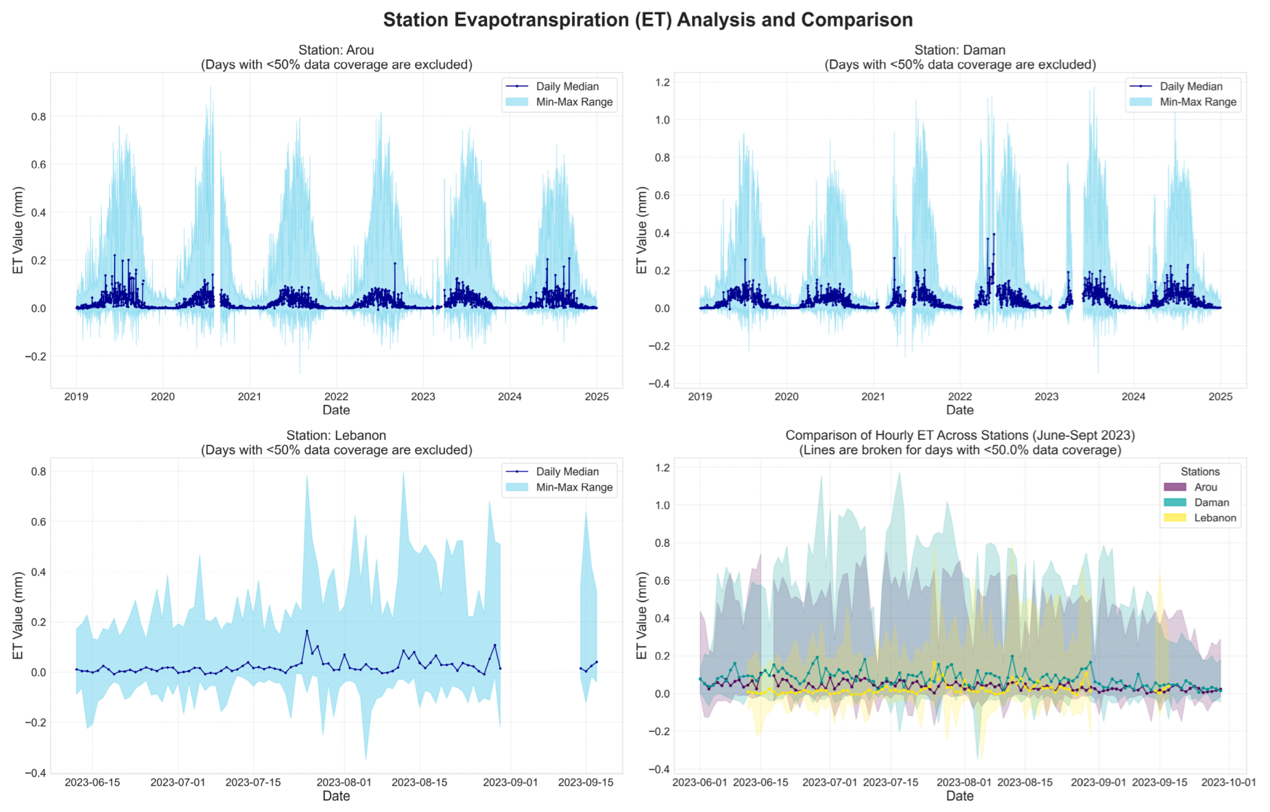
Figure 2 presents the observed evapotranspiration (ET) values from eddy covariance (EC) measurements. The ET values recorded at the Daman station in the Heihe River Basin are relatively high and, similar to those at the Arou station, exhibit a unimodal seasonal pattern, with peak vegetation evapotranspiration occurring during the main crop growing season in July and August. Due to the short period of EC records available from the Bekaa Valley station in Lebanon, it is not possible to capture the full annual variation in actual evapotranspiration. Nevertheless, a comparison reveals that the ET value at the Lebanese station increased significantly in August, exceeding that in July and reaching a level comparable to the ET values observed in the same month at both the Daman and Arou stations.

2.2. Remote Sensing and Reanalysis Data

The remote sensing data used in this study come from Sentinel-2. We selected a level 2 surface reflectance product and processed the data through the Google Earth Engine (GEE) platform, mainly including data screening and cloud removal, to obtain the blue, green, red, and near-infrared band reflectance at a resolution of 10 m after cloud masking, with a time interval of 5 days.

Near-Infrared Reflectance of Vegetation (NIRv) is a remote sensing indicator used to characterize the photosynthetic activity of vegetation (Equation (1)). It is calculated by multiplying the Normalized Difference Vegetation Index (NDVI) with the Near-Infrared Reflectance (NIR).

NIRv = NDVI × NIR

(1)

NDVI reflects vegetation coverage and growth status through the calculation of red and near-infrared reflectance; NIR directly reflects the reflection characteristics of vegetation in the near-infrared band. Research has shown that NIRv, as a proxy indicator of vegetation photosynthesis, has a better correlation with total primary productivity (GPP) than solar induced chlorophyll fluorescence (SIF), and performs more robustly in estimating evapotranspiration (ET) and reference evapotranspiration (ETo) [33]. Therefore, this article ultimately selected three remote sensing indicators, namely blue and green reflectance and NIRv, for the training of subsequent models.

In order to solve the problems of cloud pollution and time gaps in remote sensing data, this paper used an improved approach penalized least square regression based on discrete cosine transform (DCT-PLS) [34]. The method was used to reconstruct the reflectance and vegetation index over time, obtaining daily cloudless blue and green reflectance and NIRv remote sensing data for subsequent hourly ET mapping. The algorithm code is publicly available on the Google Earth Engine platform (https://code.earthengine.google.com/ac1878091de6f5879b072ab322d45053, accessed on 1 June 2024) and can be used to generate reconstructed cloud-free images at 10 m resolution, supporting applications in land use, urban development, agriculture, and ecosystem studies. We input the Blue and Green bands and NIRv index calculated every five days from Sentinel-2 in the research area into the algorithm, and obtain daily reconstruction results.

This study used ERA5 Land reanalysis data, released by the European Centre for Medium-Range Weather Forecasts (ECMWF), as the meteorological elements required for evapotranspiration estimation, mainly including: 2 m dew point temperature (d2m), 2 m air temperature (t2m), atmospheric surface pressure (sp), 10 m u-component (zonal) of wind speed, 10 m v-component (meridional) of wind speed, surface net solar radiation, surface net thermal radiation. The net radiation Rn was calculated from surface net solar radiation and surface net thermal radiation, and wind speed was calculated from zonal and meridional wind speeds. These meteorological elements are usually necessary parameters in calculating evapotranspiration [35]. This study obtained ERA5 Land data within the study area and resampled it to 10 m using bilinear method.

2.3. Machine Learning Approach

We used the Extreme Gradient Boosting (XGBoost) machine learning algorithm, which is a supervised regression model based on the Gradient Boosting Decision Tree (GBDT) framework that improves model performance through regularization optimization and parallel computing [18]. The core advantage of XGBoost lies in its strong fitting ability for nonlinear relationships, as well as its ability to effectively suppress overfitting through mechanisms and tree pruning. These characteristics make it perform well in handling ecological hydrological data with multiple features and scenarios. 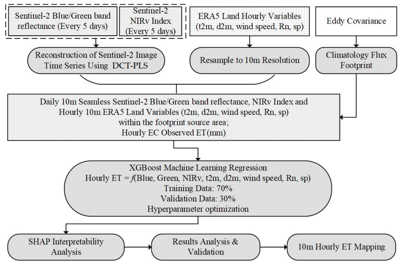Figure 3 shows the framework of the entire study.

In this study, the training data for the XGBoost model were obtained from hourly resolution observations of ET from the above three flux towers, as well as remote sensing data (blue, green, NIRv) extracted from the footprint source area of the flux towers and ERA5 Land meteorological elements. Due to the limited observation period at the Lebanese station and the lack of representativeness of its climatological footprint, we utilized the remote sensing pixels corresponding to the latitude and longitude positions of the site.

By using data from three different sites, it is possible to cover a wider range of geographic heterogeneity, vegetation types, and microclimate conditions, thereby enhancing the model’s adaptability to complex underlying surfaces at the regional scale and reducing potential systematic biases in single site data.

2.4. Evaluation Method

The coefficient of determination (R²), the root mean square error (RMSE), Nash–Sutcliffe efficiency(NSE), and percent bias (PBias) were selected to evaluate model performance [36]. The coefficient of determination (R²) reflects the collinearity between simulated and observed data. RMSE quantifies the prediction error in the units of the variable of interest. NSE is a normalized statistic that represents the proportion of residual variance relative to the variance of the observed data; it indicates how closely the simulated versus observed values align with the 1:1 line. The Percent bias (PBias) measures the average tendency of the simulated data to be larger or smaller than their observed counterparts.

3. Results and Discussion

3.1. ET Validation

The XGBoost adopts an additive model of gradient-boosted trees, which is capable of handling non-linear relationships and interaction terms, and is relatively robust to heteroscedasticity and outliers. In this study, 96,957 hourly observed ET data were used for model training, combined with remote sensing data and ERA5 data. A grid search was employed to optimize the hyperparameters, including n_estimators, learning_rate, max_depth, subsample, and colsample_bytree, with the negative mean squared error as the evaluation metric. Finally, the optimal parameters were obtained (

Table 1. The optimal values of XGBoost hyperparameters.

Hyperparameters	Optimal Value	Description
n_estimators	150	Number of boosting rounds (trees)
learning_rate	0.2	Shrinks the contribution of each tree to prevent overfitting
max_depth	7	Maximum depth of a tree
subsample	1	Subsample ratio of the training instances for each tree
colsample_bytree	0.8	Subsample ratio of features for each tree

).

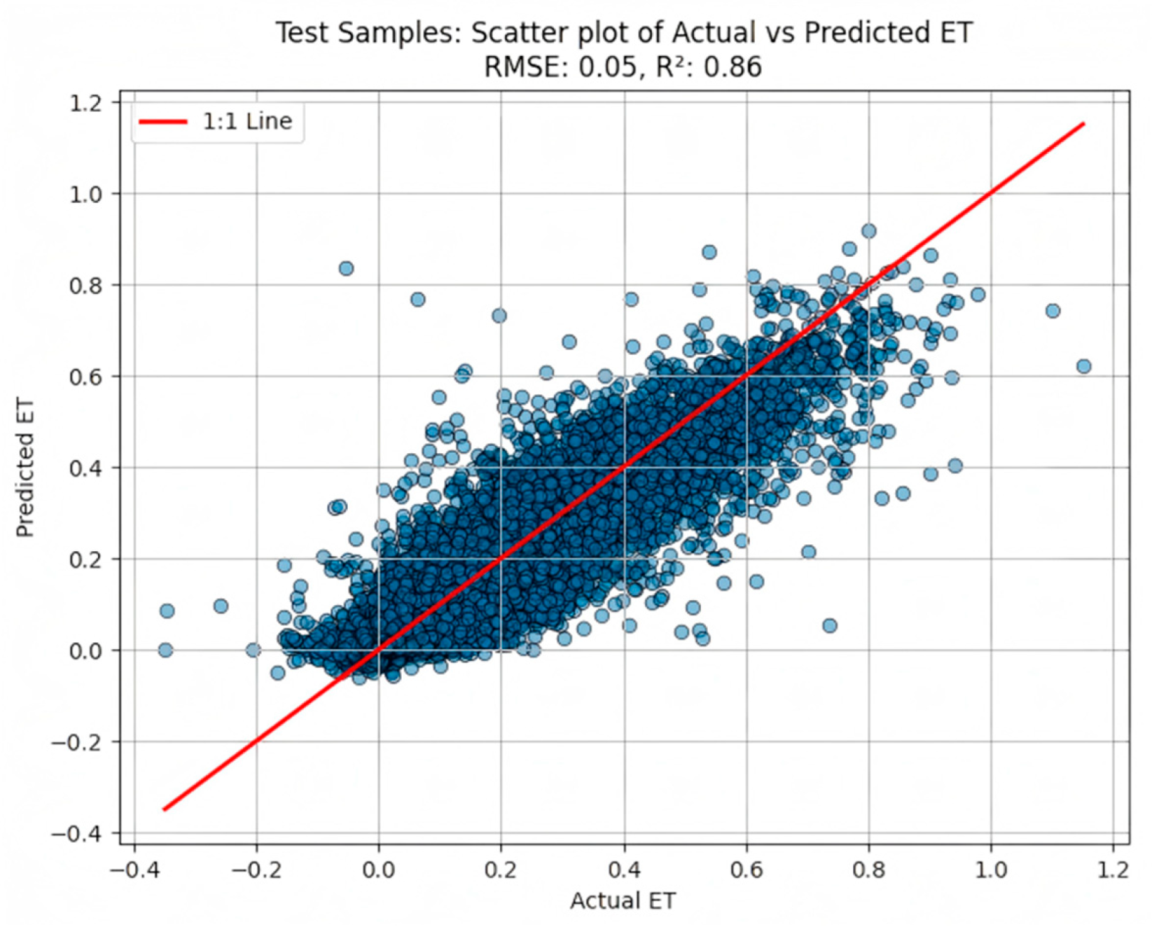
After the model training was completed, we validated it on the test set using 29,088 hourly ET data points (Figure 4). The results showed that the hourly ET simulated by XGBoost was in excellent agreement with the actual observations, with a coefficient of determination (R²) reaching 0.86 and a root mean square error (RMSE) of 0.05 mm/h.

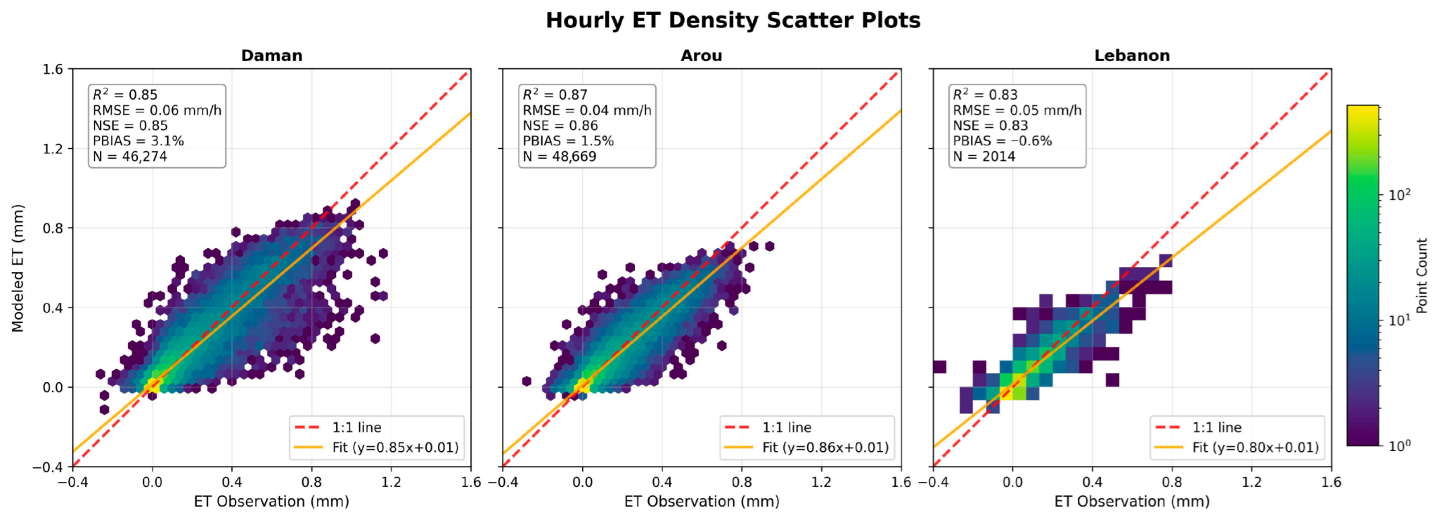
We further analyzed the simulation performance at each station and plotted density scatter plots of all predicted versus observed ET values for the model, and calculated the aforementioned evaluation metrics (as shown in Figure 5). The results indicated that the trained model performed well at each station and was capable of estimating hourly evapotranspiration under different underlying surface conditions. Although the Lebanon station had a shorter observation period and fewer training samples compared to the other two stations, it still achieved favorable estimation results. For the three stations, the coefficients of determination ranged from 0.83 to 0.87, the root mean square errors ranged from 0.04 to 0.06 mm/h, the Nash–Sutcliffe efficiency (NSE) coefficients were relatively high, ranging from 0.83 to 0.86, and the percentage bias (PBias) ranged from −0.6% to 3.1%. These metrics collectively confirm the effectiveness of this machine learning model. Due to the lack of long-term EC observations at the Lebanese site, it is not possible to calculate the long-term climatological footprint. As it is a relatively uniform underlying surface of farmland, we used ET pixels at the latitude and longitude positions of the site for validation. Previous studies have also achieved good ET validation results in these regions on a daily scale [29,37]. However, this article focuses on validation and discussing from the perspective of high spatio-temporal (10 m, hourly) resolution ET.

3.2. SHAP Interpretability Analysis

To investigate the complex nonlinear relationships within the XGBoost evapotranspiration (ET) prediction model, this study employed the SHAP (SHapley Additive exPlans) method based on game theory for explanatory analysis of the model. The SHAP method not only quantifies the contribution of each input feature to a single prediction (SHAP value), but also further reveals the interaction effects between features [38].

3.2.1. Importance of Features

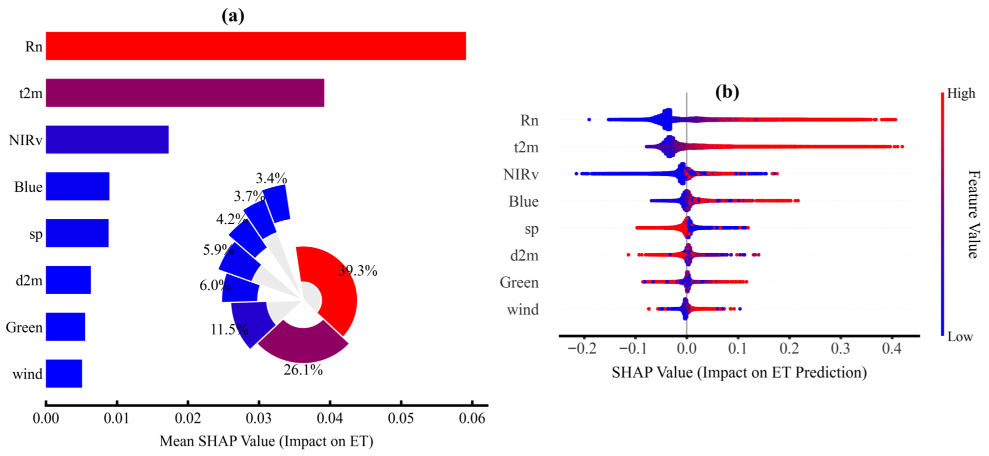
First, we evaluated the global importance of each input feature by computing the mean absolute SHAP value across all samples. The analysis revealed the following percentage contributions to the model’s predictions: Rn (39.3%), t2m (26.1%), NIRv (11.5%), Blue (6.0%), sp (5.9%), d2m (4.2%), Green (3.7%), and wind (wind speed) (3.4%) (Figure 6a). The dominance of Rn aligns with the energy-limited mechanism: during the daytime, the available energy supply directly governs the partitioning of latent heat flux. When water is not extremely scarce, an increase in Rn necessarily enhances the potential for ET. The secondary importance of t2m reflects the combined influence of air temperature on the vapor pressure deficit and turbulent exchange; together with d2m and sp, it characterizes the atmospheric aridity and pressure background.

The importance of NIRv is also relatively high, and it is generally superior to individual near-infrared bands or NDVI in highlighting the tight coupling between vegetation’s photochemical absorption and its transpiration flux. Blue/Green reflectance may indirectly reflect water stress and structural information through atmospheric and leaf optical properties. Although wind ranks lower in importance, it may amplify the conversion efficiency of energy into latent heat under extreme conditions.

The beeswarm plot in Figure 6b indicates that high values of Rn and t2m correspond with a large number of positive SHAP values, confirming that an increase in these features generally drives ET predictions upwards. In its higher range, sp exhibits some negative SHAP values, which may be related to air density and turbulence characteristics in low-altitude/high-pressure environments. In its lower range (drier air), d2m is more prone to negative SHAP values, reflecting the complexity where ET can be limited by an vapor pressure deficit (VPD) [39], it is a phenomenon that typically requires joint interpretation with t2m and Rn.

3.2.2. SHAP Dependence Analysis

To precisely dissect the details within these general trends, we generated SHAP dependence plots for each key feature. As shown in Figure 7, these plots display the physical value of a feature on the x-axis, with a background histogram representing the distribution of its values. The corresponding SHAP value is shown on the y-axis, and a LOWESS (Locally Weighted Scatterplot Smoothing) curve is fitted to clearly delineate the average trend of the feature’s marginal effect (contribution to ET prediction). This approach helps to reveal the highly non-linear, univariate response patterns learned by the model.

The marginal contribution of net radiation (Rn) grows steadily with its value, indicating the positive marginal benefit of energy supply on ET. In contrast, 2-m temperature (t2m) exhibits a strong threshold effect, where its positive driving impact on ET only becomes rapidly apparent after the temperature exceeds approximately 283 K. The 2-m dewpoint temperature (d2m) exhibits a subtle inverted U-shaped relationship, indicating that the model accurately captured the physical process in which excessively high air humidity reduces the vapor pressure deficit, thereby suppressing ET. The dependence plot for surface pressure (sp) shows a distinct multi-modal distribution, which provides compelling evidence that the model did not learn a single pressure response. The model effectively captures the distinct climate patterns caused by altitude variations across different sites, establishing unique responses for high and low-pressure systems. While the overall influence of wind speed is less pronounced and relatively stable, the model correctly identifies its positive effect above approximately 1.6 m/s, where it enhances surface-atmosphere moisture exchange.

The influence of NIRv also exhibits a threshold, beginning to contribute positively to ET only after the vegetation index exceeds approximately 0.11, which reflects the relationship between vegetation “greenness” and transpiration activity. In comparison, the marginal contribution trend lines for the Blue and Green band reflectances are almost perfectly aligned with the zero line. This suggests that the information within these two bands may be redundant, as their effective representation of vegetation status has been encompassed and superseded by the more powerful vegetation index (NIRv).

3.2.3. Analysis of Feature Interaction Effects

To reveal the multivariate coupling mechanisms driving changes in Evapotranspiration (ET), we calculated the SHAP interaction values. The numerical values in the generated heatmap (Figure 8) represent the mean absolute SHAP interaction value for each pair of features. It quantitatively identifies that the strongest interaction in the model occurs between net radiation (Rn) and NIRv, with an average interaction strength of 0.010, followed by the interaction between Rn and 2-m air temperature (t2m) at 0.008. A detailed analysis of the two strong interaction pairs reveals profound synergistic mechanisms:

The interaction diagram between Rn and NIRv reveals a more complex mechanism. Under high NIRv (dense vegetation) conditions (red trend line), the marginal effect of Rn is significantly steeper than under low NIRv (sparse vegetation) conditions (blue trend line).This decisively demonstrates that the model has identified vegetation as the primary medium for converting surface energy into water flux. Energy input can only be efficiently transformed into evapotranspiration (ET) when it encounters vegetation capable of vigorous transpiration. When vegetation is dense, an increase in net radiation (Rn) significantly boosts ET. Energy (Rn) and vegetation (characterized by NIRv) exhibit a strong synergistic effect. The higher the Rn, the stronger the transpiration of vegetation, and the higher the interaction SHAP value. However, when vegetation is sparse, an increase in Rn actually suppresses ET. In areas with low vegetation cover, the main evaporation comes from the soil surface. When Rn is low (such as in the morning), there is still a certain amount of moisture in the soil surface that can be evaporated. But with a sharp increase in Rn (such as at noon), the strong energy input will quickly dry the soil surface, forming a dry hard shell. This dry surface layer will hinder the evaporation path of lower soil moisture, and instead lead to a decrease in overall evaporation. Therefore, the model learned an antagonistic effect: for bare soil or sparse vegetation, excessive energy input (high Rn) will have a negative interaction on ET through rapid evaporation of the surface layer.

The interaction between Rn and t2m is particularly revealing of the model’s ability to capture complex biophysical feedbacks. While a synergistic effect (positive interaction SHAP values) is observed under moderately high energy and temperature, this relationship reverses under extreme conditions (Rn > 300 W/m² and t2m > 275.97 K), where the interaction becomes negative. This physical mechanism of water limitation provides a compelling explanation for this phenomenon. The combination of high radiation and high temperature creates a significant vapor pressure deficit (VPD), inducing water stress and subsequent stomatal closure in vegetation as a self-preservation response. The model has successfully learned from the data that under these extreme “double high” conditions, the actual ET is suppressed below what would be expected from the additive effects of the individual drivers. The model’s ability to capture this critical feedback loop, where atmospheric demand can trigger a surface resistance that limits ET, demonstrates its power in simulating real-world, non-linear ecohydrological processes.

Overall, the SHAP-based interaction analysis reveals not only the statistical coupling between climatic and biophysical variables but also physically interpretable ecohydrological feedbacks, such as the transition between energy- and water-limited regimes, stomatal regulation under high VPD, and the soil-vegetation partitioning of evaporation and transpiration.

3.3. Mapping 10 m Hourly ET

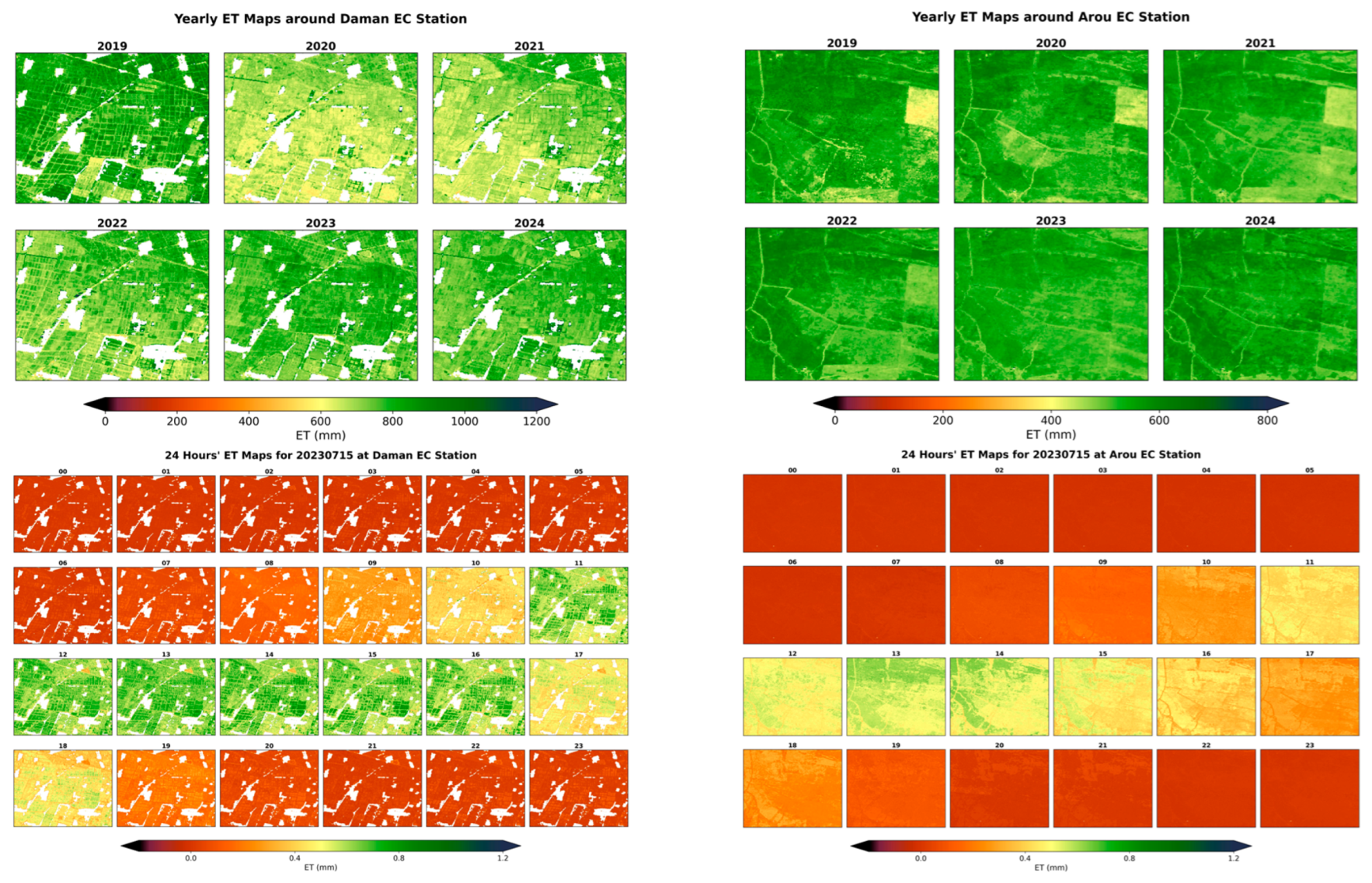
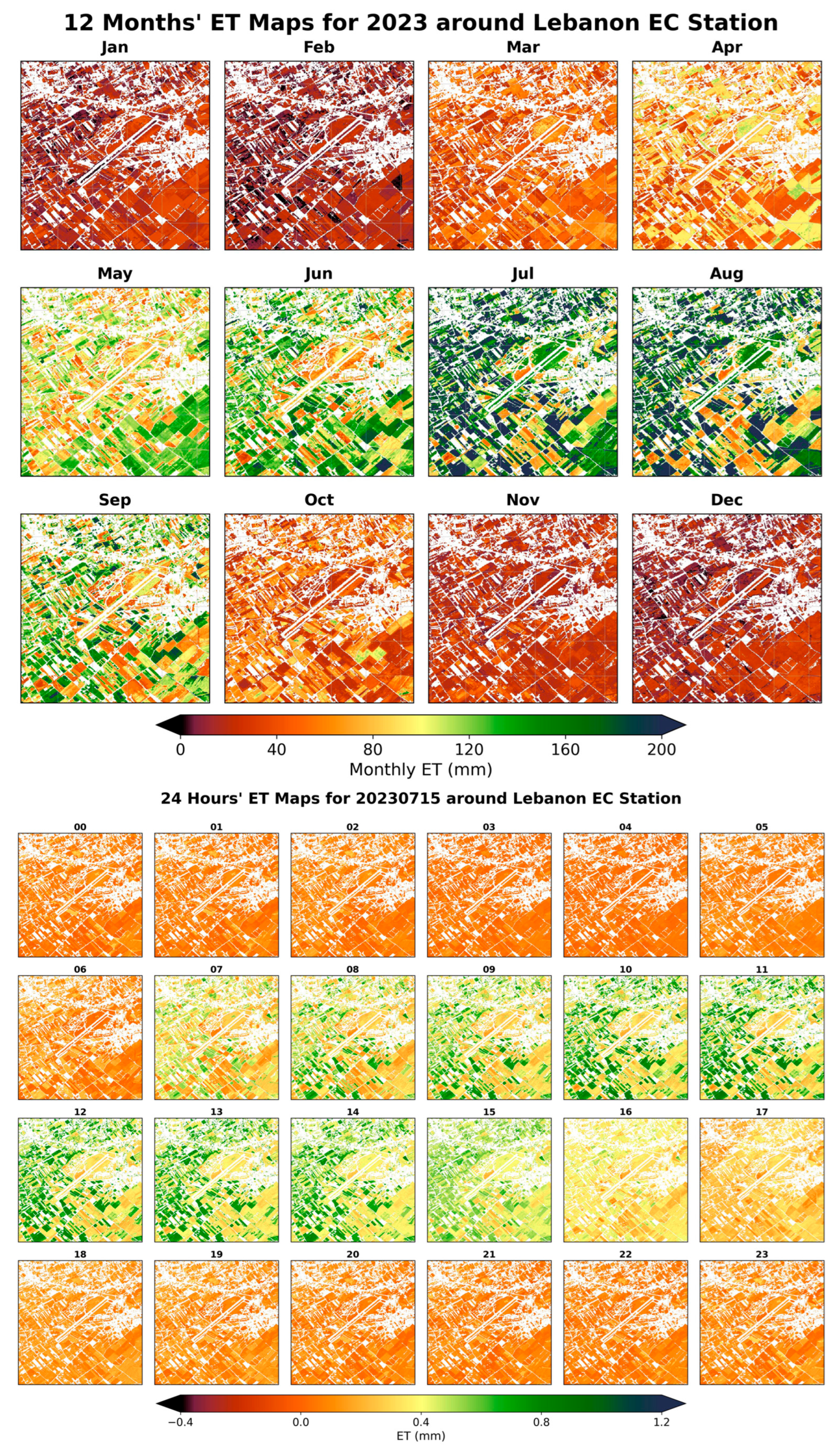
To validate the application potential and robustness of the constructed XGBoost model at the regional scale, we utilized the model to generate 10-m high-resolution evapotranspiration (ET) maps for vegetation areas around three typical sites (Figure 9 and Figure 10). The results were visualized and analyzed across multiple temporal scales, including interannual, monthly, and diurnal variations.

The annual-scale ET maps clearly revealed the spatial heterogeneity of vegetation ET and its interannual variability. The annual total ET of cropland at the Daman site exceeded 1000 mm, reflecting the contribution of vegetation transpiration to the regional water cycle. The overall high ET areas in the eastern part of the Arou site from 2022 to 2024 were significantly higher than those from 2019 to 2021. These multi-year scale maps demonstrated the model’s ability to stably capture the macro-scale spatiotemporal dynamics of ET driven by land use and interannual climate fluctuations.

The monthly ET maps for the Lebanon site showcased the model’s capability to capture seasonal cycles. From January to March, regional ET generally remained at low levels (<40 mm/month), consistent with low winter temperatures and the vegetation dormancy period. Starting in April, as temperatures rose and vegetation resumed growth, ET in farmland areas increased rapidly, peaking during the peak growing season from June to August (>160 mm/month). The maps clearly distinguished the asynchronous ET increases among different crop plots due to phenological differences. Starting in September, as crops matured and were harvested, ET gradually decreased, reaching winter levels by December. This complete seasonal evolution process was highly consistent with regional agricultural phenology and climate cycles, confirming the model’s precise simulation capability for dynamic surface processes.

The hourly ET maps of the three sites on 15 July 2023 show the diurnal variation pattern of ET. At night (around 20:00 to 06:00 the next day), ET is close to zero, which conforms to the physiological law of interrupted energy input and closed stomata at night. Morning (around 07:00 to 11:00): As the sun rises, ET begins to rapidly increase; Afternoon (around 12:00 to 16:00): ET reaches its intraday peak, with the most significant spatial heterogeneity. At this point, the differences in crop types and irrigation conditions have led to significant variations in ET between plots. Evening (around 17:00 to 19:00): As solar radiation decreases, ET begins to rapidly decline and returns to extremely low levels after sunset. The 24-h dynamic evolution not only presents a typical “unimodal” daily variation curve in time, but also maintains a high degree of consistency with the land cover pattern in space.

4. Conclusions

This study developed a method to estimate hourly agricultural evapotranspiration (ET) using machine learning. The model, based on the XGBoost algorithm, combined Sentinel-2 satellite data, ERA5-Land weather data, and ground observations from three agricultural sites. Model validation showed a high level of agreement between the estimated hourly ET and the actual observed values.

A key novelty of this work lies in leveraging the explainable machine learning tool (SHAP) to explicitly uncover and quantify the key controlling factors of hourly ET, as well as their nonlinear relationships and interaction effects. This analysis showed that net radiation (Rn), 2-m air temperature (t2m), and a vegetation index (NIRv) were the most important factors for estimating ET. SHAP also revealed important interactions. For example, the combination of high net radiation and healthy vegetation (high NIRv) led to a large increase in ET, showing that vegetation is key to converting energy into ET. It also found that under conditions of high radiation and very high temperatures, ET was suppressed, which reflects how plants close their stomata to conserve water.

The model was used to produce hourly ET maps at a 10-m resolution. The mapping results at interannual, monthly, and diurnal scales all exhibited spatiotemporal dynamics highly consistent with actual surface processes. These maps can be used for practical applications like improving irrigation scheduling and regional water management.

Future work should test the model’s performance in a wider range of regions and with different crop types to assess its transferability. The model could also be improved by including soil moisture data as an input, which would be particularly valuable for improving the accuracy of ET estimation when vegetation cover is low. In addition, future research will also focus on integrating the proposed hourly ET estimation framework into practical applications, such as precision irrigation scheduling and regional water resource accounting, to further evaluate its operational potential.