Research on Driving Forces of Spatiotemporal Patterns in Cotton Cultivation Considering Spatial Heterogeneity

Abstract

Cotton is increasingly important in global development. The exploration of drivers of spatiotemporal patterns for cotton planting, considering spatial heterogeneity, is essential for optimizing its distribution and supporting sustainable production. This study combined the locally explained stratified heterogeneity (LESH) model with geographically weighted regression (GWR) to investigate the factors shaping cotton-planting patterns in the northern slope of the Tianshan Mountains (NSTM), China, from 2000 to 2020. Cotton distribution was derived from long-term Landsat image series, and its expansion showed an average annual growth rate of 2.10 × 10³ km², with intensive cultivation primarily distributed across the central and western counties. The dominant drivers of cotton distribution were elevation (ELE), sunshine duration (SD), slope (SLO), temperature (TEM), runoff (RO), and gross domestic product (GDP). ELE explained about 40% of the spatial heterogeneity. SD showed a declining influence, SLO remained stable, TEM increased in importance, and GDP exhibited a progressive upward trend, although weaker. Moreover, nonlinear weakening interactions, especially between ELE and other factors, as well as between socio-economic and climatic variables, substantially enhanced explanatory power. These findings highlight the significance of accounting for spatial heterogeneity and factor interactions in guiding the spatial optimization and sustainable management of cotton cultivation.

1. Introduction

Cotton, as a key economic crop, plays a crucial role in the global textile industry, serving as the primary source of natural fibers for textile production worldwide. With the continuous growth of the global population, the demand for cotton has shown a steady upward trend [1]. Cotton is cultivated across Asia, Africa, the Americas, Europe, and Oceania. China ranks among the world’s leading producers and consumers of cotton, maintaining a dominant position in global output. In 2022, China accounted for 24% of global cotton production [2]. However, existing research on cotton cultivation has mainly focused on yield estimation, climate suitability assessment, and remote sensing identification of cotton areas. Relatively few studies have systematically examined the spatiotemporal evolution and driving mechanisms of cotton distribution across multiple spatial scales. Moreover, many driver-focused studies remain at a single, large scale, and the interactions among multiple driving factors are often unclear, which limits the explanatory power of their results. Studies also tend to emphasize global or regional trends without integrating local spatial heterogeneity in depth. Addressing these gaps is essential for improving the interpretability of driving factors and for guiding the spatial optimization and sustainable management of cotton production. Similar challenges are present in studies conducted in China, and particularly in Xinjiang. Cotton research in these regions also tends to overlook multi-scale spatiotemporal dynamics and the interactive effects of multiple environmental and socio-economic drivers. Xinjiang has the largest planting area and the highest total output of cotton in China. The northern slope of the Tianshan Mountains (NSTM) is the most-developed region of Xinjiang and has become a crucial production area for high-quality cotton in China because of superior sunlight conditions and abundant water resources from the melting snow of the Tianshan Mountains. The plots for planting are small, numerous, scattered, and irregular in shape, although the cotton planting area in Xinjiang is large. This greatly increases difficulties in the collection of information, and makes the work of statistics and the verification of planting areas difficult, resulting in poor timeliness and accuracy of statistical data. Therefore, extracting long-term cotton distribution information using remote sensing and assessing spatiotemporal evolution and its driving mechanisms at multiple scales are both necessary.

The development and evolution of spatial patterns of cotton cultivation is a complex process, shaped by the combined effects of multiple factors. Previous studies have reported that changes in the spatial distribution of cotton production are influenced by natural resource endowments, production inputs, socio-economic conditions, technological advances, market demand, policy interventions, and other related factors [3]. Research on the driving forces of spatiotemporal changes in crop distribution involves qualitative or quantitative analysis of both internal and external factors underlying spatial crop variations, aiming to determine the relative contributions of different drivers for the formation of crop spatial patterns. Common research methods include descriptive statistics [4], gray relation theory [5], regression analysis [6], interpretable machine learning [7], and spatial econometric models [8], etc. Among them, widely applied spatial econometric methods focus on exploring the impacts of socio-economic factors on spatiotemporal distributions of cotton planting, taking into account the spatial spillover effects of crop planting between regions, spatial heterogeneity, and interaction among factors. Anthropogenic factors, such as economic conditions, policy orientations, and technological advancements, directly determine farmers’ cultivation practices and agricultural production processes. Meanwhile, these factors further indirectly alter the spatial distribution of crop cultivation by influencing both natural resource utilization and collective decision-making behaviors in planting activities. However, this method relies on spatial panel data with the smallest spatial scale of county level. Cotton cultivation falls under the category of agricultural production with a process of natural reproduction. Therefore, natural resource conditions are the foundation and prerequisite for the formation and changes in layout of agricultural district distribution. Land plots used for cotton production vary in size from tens of kilometers to a few meters. This aligns with the laws of geography and exhibits spatial heterogeneity and dependence. Therefore, research on the influential mechanism of spatiotemporal distribution changes in cotton from the view of spatial heterogeneity contributes to a systematic and accurate analysis of driving forces behind cotton production, particularly the function mechanism of natural factors on cotton cultivation.

Geospatial analytical methods, consisting of linear and nonlinear models, are commonly employed to investigate the driving of spatial variability in geographical variables. Geographically weighted regression (GWR) is a common linear method for analyzing local spatial non-stationarity of variables [9]. GWR can more accurately capture localized patterns in spatial data by variations in variable regression coefficients with spatial position. However, it only evaluates linear relationships between variables and lacks the ability to examine global patterns or explore interactions among multiple factors. Spatially stratified heterogeneity (SSH) models are effective analytical frameworks for characterizing the spatial variability of geographical variables in a nonlinear way [10]. These models measure the spatial distribution patterns of variables using the power of determinants (PD). Higher PD values indicate that similar spatial distributions exist in variables and that factors have stronger explanatory power over response variables. However, PD calculated by the classical SHH model is significantly underestimated if optimization of the spatial discretization is not conducted and does not adequately explain the spatial correlations between the explanatory variables and response variables. Some studies have focused on optimizing spatial discretization processes to address this problem. For instance, the concept of optimal power of determinants (OPD) has appeared in geographical detector and geographically optimal zones-based heterogeneity models (GOZH), aiming to improve the representation of spatial association [11]. These methods can not only quantify the influence of individual factors on the spatial distribution of response variables but also reveal the interactive effects of multiple factors. However, the specific contribution of each factor within these interactions remains unknown. Fortunately, the Shapley Additive Explanations (SHAP) model, with its unique theoretical foundation, makes models explanatory, and fairly distributes the contribution of each feature to the output of models [12]. Li et al. proposed a locally explained stratified heterogeneity (LESH) model with SHAP that well overcomes the black-box problem existing in current SSH models [13]. This model can determine the contribution of each explanatory variable and interactions among multiple variables by calculating the SHAP power of determinants (SPD). However, these SSH models are unable to reveal local spatial variations in variables.

Based on the above analysis, this study addresses the following objectives: (1) To generate a long-term time series of cotton cultivation patterns using remote sensing technology. (2) To characterize the spatiotemporal evolution and regional differentiation of cotton cultivation. (3) To explore the driving forces behind the spatiotemporal variations in cotton cultivation and quantify the contributions of both global- and local-scale factors.

2. Materials and Methods

2.1. Study Area

The NSTM is situated in the inland center of the Eurasian continent with an area of approximately 3.96 × 10⁵ km² (40°52′–47°14′ N, 79°53′–96°23′ E), accounting for 23.8% of Xinjiang’s total area [14], as shown in Figure 1. The NSTM, as a national second-tier key urban agglomeration, is a center of population, industry, and economy and a core hub linking China with Central and West Asia due to its favorable resource endowments and strong economic foundation [15,16]. The region is characterized by a higher altitude in the south than the north and has an altitude ranging from −153 m to 4814 m [17]. It has a typical temperate continental arid climate, with an average annual precipitation of approximately 115 mm and an average annual temperature of about 9.8 °C [18]. In short, it is one of the major cotton producing areas in Xinjiang because of its abundant light and heat. Additionally, the NSTM has typical oasis agricultural cultivation areas of Xinjiang, with the main planted crops of cotton, maize, and wheat. Their growth stages mainly span from April to October, as is shown in Figure 2. Accurately understanding the phenological stages of these crops helps in selecting the appropriate temporal windows of remote sensing imagery for extracting crop distribution information. Cotton in the NSTM is sown in the middle or late part of April each year, then goes through the stages of emergence, seedling, square, boll, and open boll, and is finally harvested in October, when other crops have largely been harvested.

2.2. Data Source

2.2.1. Satellite Data

To ensure both long-term continuity and suitable spatial resolution for cotton mapping, this study employed Landsat-5 thematic mapper (TM) and Landsat-8 operational land imager (OLI) imagery to extract the cotton area in 2000, 2005, 2010, 2015, and 2020. The Landsat series provides consistent global coverage with a spatial resolution of 30 m, making it well suited to monitoring long-term agricultural changes. The combination of TM and OLI sensors ensures the comparability and continuity of spectral characteristics across time. Except for the thermal infrared band, all spectral bands were used for cotton extraction to enhance classification accuracy. Moreover, high-resolution remote sensing imagery from certain years and regions was also used to obtain sufficient and accurate samples required for cotton extraction (

Table 1. Information of remote sensing image data.

Number	Satellite	Time Phase	Range	Spatial Resolution
1	Landsat-5	September 2000, 2005, and 2010	Study area	30 m
2	Landsat-8	September 2015 and 2020
3	GF-1	2 September 2015, 10 September 2015	Changji and Urumqi	2/8 m
4	GF-2	9 May 2020, 2 August 2020, 16 August 2020	Qitai County, Wenquan County and Shihezi City	1/4 m
5	GeoEye-1	16 July 2010	Shuanghe City	0.41/1.64 m
6	QuickBird	28 August 2002 17 May 2006	Wujiaqu City and Hami City	0.61/2.44 m

).

2.2.2. Sample Data

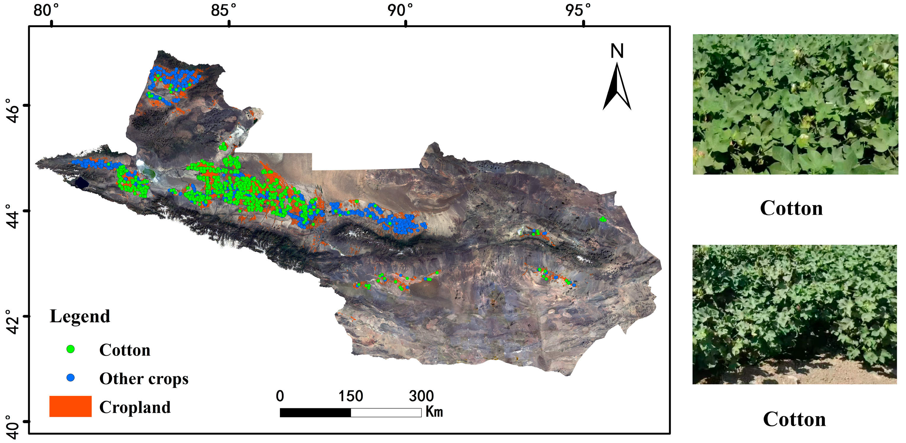
Sample points used for the remote sensing extraction of cotton were primarily obtained through field survey and visual interpretation. The field survey data included unmanned aerial vehicle images with high spatial resolution covering the typical cropland of Xinjiang in 2020 and scientific investigation data from 2023 [19]. In addition, the sample data of crops in each year are from high spatial resolution images in GF-2, Sentinel-2, GF-1, QuickBird, GeoEye-1, and Google Earth, obtained by visual interpretation. Owing to the scarcity of historical field survey data, the sample dataset in 2020 was initially established based on scientific surveys, unmanned aerial vehicle imagery, and high spatial resolution images. Sample points in other years were obtained by referring to the sample distribution from the year 2020 and combining high spatial resolution imagery with Google Earth data (Figure 3).

2.2.3. Factors Selected

Selected variables that may affect spatiotemporal variations in cotton-planting patterns include five categories: topography, climate, soil, water resources, and socio-economy (

Table 2. Selected explanatory variables.

Category	Variable	Abbr.
Topography	Elevation	ELE
	Slope	SLO
Climate	Temperature	TEM
	Precipitation	PRE
	Wind speed	WS
	Sunshine duration	SD
Soil	Soil type	ST
Water resources	River network	WAT
	Evaporation	EVA
	Runoff	RO
Socio-economy	Gross domestic product	GDP

). Topographical variables consist of elevation (ELE) and slope (SLO), representing the terrain conditions for cotton cultivation. ELE is derived from the advanced spaceborne thermal emission and reflection radiometer global digital elevation model (ASTER GDEM V2), with a spatial resolution of 30 m. The dataset is provided by the Geospatial Data Cloud site, the Computer Network Information Center, and the Chinese Academy of Sciences [20]. SLO is calculated based on the elevation data using spatial analysis methods.

Climate is a fundamental driving force influencing the spatiotemporal variations in cotton cultivation, directly affecting the growth, quality, and yield of cotton. Climate variables used include temperature (TEM), precipitation (PRE), wind speed (WS), and sunshine duration (SD). TEM, PRE, and WS were derived from the ERA5-Land monthly averaged data [21]. ERA5-Land is the land reanalysis data, with a spatial resolution of 0.1°, produced by the European Centre for Medium-Range Weather Forecasts, which integrates multi-source observations with numerical models. The SD data was collected from the National Earth System Science Data Center and the Science Data Bank [22,23,24,25]. The former provides the monthly sunshine duration data, with a spatial resolution of 1 km. The data from 2000, 2005, 2010, and 2015 was used for this study. These datasets were generated via the spatial interpolation of thin plate spline, based on the data from ground reference and meteorological stations. The latter provides the daily mean sunshine duration datasets in 2020 for this study, derived from Himawari-8 shortwave radiation products.

The soil type (ST) data come from the Resource and Environmental Science Data Platform [26]. This data was digitally generated from the soil map of the People’s Republic of China, with a scale of 1:1,000,000, and has the basic mapping unit of subclass.

Water is the factor that guarantees the high yield and quality of cotton. The variables concerning water resources include river network (WAT), evaporation (EVA), and runoff (RO). The WAT data were obtained from the Data Sharing and Service Portal, with a temporal resolution of 5 years/period and a spatial resolution of 30 m [27]. EVA and RO were collected from the ERA5-Land monthly averaged data.

Gross domestic product (GDP) is a monetary measure of the market value of all the final goods and services produced within a specific period [28]. It is one of the important indicators of social and economic development, influencing the layout, scale, and technical levels of the cotton planting industry through multiple pathways. The data from the Resource and Environmental Science Data Platform were acquired based on the spatial interaction of land use, nighttime light intensity, residential density, and GDP statistical data, using the method of multi-factor weight distribution.

2.2.4. Other Data

The vector data of administrative divisions in the study were obtained from the Xinjiang Uygur Autonomous Region Platform for Common Geospatial Information Services [29]. The datasets of cultivated land with a spatial resolution of 30 m in the NSTM from 2000 to 2020 were used for the masking of images and the extraction of cultivated land [30]. The statistical data of the cotton-sown area in the NSTM from 2000 to 2020 were sourced from related statistical yearbooks: the Xinjiang Statistical Yearbook and the Xinjiang Production and Construction Corps Statistical Yearbook.

2.3. Methods

2.3.1. Remote Sensing Extraction of Cotton

To accurately acquire distribution information on cotton from 2000 to 2020, this study selected September as the optimal time phase for remote sensing based on the phenological characteristics of cotton, while also considering the quality and availability of remote sensing data, and then used cultivated land data to mask images. On this basis, cotton planting information from various different years was obtained from the time series Landsat images during this optimal phase using the random forest (RF) algorithm on the Google Earth Engine (GEE) platform. RF is an ensemble machine learning algorithm that combines bagging and random subspace methods. It builds multiple decision trees on bootstrapped samples and integrates their results to produce the final prediction. This improves its generalization ability and performance in handling nonlinear relationships and multivariate data. Compared with other algorithms, such as support vector machines (SVMs), this algorithm with a tree structure does not rely on distance calculation and does not require feature scaling [31]. The optimal classification model was determined by a number of trials, while the initial values of number of trees, leaf nodes, tree depth, and maximum number of iterations in the RF were set to 200, 10, 25, and 150, respectively. All samples were randomly split into 70% for the training set and 30% for the validation set.

Remote sensing features and terrain are the input variables of the RF algorithm. Remote sensing features consist of radiation vales in the visible and near-infrared bands of the Landsat images and related multispectral vegetation indices, while the topographic variables constructed from the SRTMGL1_003 data include ELE, SLO, and aspect [32]. Selected vegetation indices are the Normalized Difference Vegetation Index [33], the Ratio Vegetation Index [34], the Enhanced Vegetation Index [35], the Difference Vegetation Index [36], and the Soil Adjusted Vegetation Index [37].

The classification models are validated from both spatial and quantitative perspectives. The confusion matrix is employed to assess the spatial accuracy of models, while the verification of cotton extraction area is based on statistical data of the cotton-sown area. The performance metrics derived from the confusion matrix are overall accuracy (OA), Kappa coefficient, producer’s accuracy (PA), and user’s accuracy (UA) [38].

2.3.2. Analytical Methods of Spatiotemporal Changes on Cotton Cultivation

This study employed the Theil–Sen median to quantify the temporal variation trends of the cotton planting area over 20 years in the NSTM. It is a robust, nonparametric method of linear regression and has strong robustness to outliers and noises [39,40]. Meanwhile, Mann–Kendall (MK) was used to test the significance of change trends. Mann–Kendall is a rank-based, nonparametric, statistical method, suitable for any time distribution pattern, with robustness, used to evaluate the randomness of the observed trends by the significance level of Z-score. Once the absolute value of the Z-score is greater than 1.65, 1.96, or 2.58, the trend passes the significance test at confidence levels of 90%, 95%, or 99% [41].

Moran’s I and Getis-Ord $G_i^{*}$ are the methods to analyze the distribution characteristics of global and local spatial clustering. Moran’s I can be used to determine the global spatial autocorrelation of cotton distribution and reflect the spatial aggregation or dispersion trends [42]. Getis-Ord $G_i^{*}$ is related to cold/hot spot analysis and can indicate spatial differentiation and significance between each element and its surrounding elements by calculating the value of the Z-score using the standardized aggregation index [43]. Regions with high-value clustering of the Z-score show the spatial aggregation distribution pattern of hot spots. The spatial aggregation distribution pattern of cold spots is shown in contrast. The spatial clustering is not significant if the Z-score approaches zero [44].

2.3.3. Methods to Reveal Drivers of the Spatiotemporal Heterogeneity of Cotton Cultivation

The joint use of LESH and GWR is a complementary approach to fully explain the influence mechanisms of selected factors on cotton-planting distributions in the NSTM. The LESH model reveals the global impact and force of factors on geographical variables from the perspective of spatial heterogeneity. It can explain the contribution of individual factors to the response variable, as well as the contribution of multi-factor interaction effects. The model uses OPD to measure the influence of individual and multiple variables on response variables. High OPD indicates strong spatial correlations between response and explanatory variables [45]. OPD is calculated as follows:

$$\mathrm{OPD}=\max (\mathrm{PD})=1-{\displaystyle \frac{\min (\mathrm{SS}{\mathrm{W}}_{\mathrm{X},\mathrm{D}})}{\mathrm{SST}}}$$

(1)

where X denotes the explanatory variable, D is the hierarchical variable describing geographical zones, and $\mathrm{SS}{\mathrm{W}}_{\mathrm{X},\mathrm{D}}$ means the sum of squares within zones that are recorded as D and determined by X.

Furthermore, an important advantage of the LESH model is that it integrates the SHAP model from cooperative game theory to calculate the contribution of each variable under interactions of multiple variables, thereby solving the black-box problem existing in the SSH models. For the explanatory variable x_j, its contribution is calculated according to the following equation:

$${\mathrm{\theta }}_{{\mathrm{x}}_{\mathrm{j}}}\left(\mathrm{S}\right)={\displaystyle \sum _{\mathrm{S}\in \mathrm{M}\backslash \left\{{\mathrm{x}}_{\mathrm{j}}\right\}}\frac{\left|\mathrm{S}\right|!\left(\left|\mathrm{M}\right|-\left|\mathrm{S}\right|-\mathrm{1}\right)!}{\left|\mathrm{M}\right|!}}\left(\mathrm{v}\left(\mathrm{S}\cup \left\{{\mathrm{x}}_{\mathrm{j}}\right\}\right)-\mathrm{v}\left(\mathrm{S}\right)\right)$$

(2)

where for the set of explanatory variables M = {x₁, x₂, x₃, …x_m} and the set S = {x₁, x₂, x₃, …x_s} (s ≤ m), S is a subset of M; S includes the empty set but not all subsets of x_j.

${\mathsf{\theta }}_{{\mathrm{x}}_{\mathrm{j}}}\left(\mathrm{S}\right)$ represents the SPD value of the explanatory variable x_j. |M| and |S| denote the number of variables in sets M and S, respectively. v(S) is an evaluation function used to calculate the OPD for |S| explanatory variables. $\mathrm{v}\left(\mathrm{S}\cup \left\{{\mathrm{x}}_{\mathrm{j}}\right\}\right)$ represents the OPD obtained by adding target variable x_j to subset S. $\mathrm{v}\left(\mathrm{S}\cup \left\{{\mathrm{x}}_{\mathrm{j}}\right\}\right)-\mathrm{v}\left(\mathrm{S}\right)$ denotes the marginal contribution, which quantifies the incremental impact on system output when the target variable x_j is added to subset S. The SPD of variable x_j is obtained by weighted summation of marginal contributions across all subsets S without x_j in M.

GWR is a method used to map out the spatial correlation within local regions. It incorporates spatial location into regression processes using a spatial weighting function, reflecting the spatial heterogeneity of geographic variables among different zones [46]. The calculation formula is as follows:

$${\mathrm{y}}_{\mathrm{i}}={\mathrm{\beta }}_0\left({\mathrm{u}}_{\mathrm{i}},{\mathrm{v}}_{\mathrm{i}}\right)+{\displaystyle \sum _{\mathrm{k}=1}^{\mathrm{p}}{\mathrm{\beta }}_{\mathrm{k}}\left({\mathrm{u}}_{\mathrm{i}},{\mathrm{v}}_{\mathrm{i}}\right)}{\mathrm{x}}_{\mathrm{i}\mathrm{k}}+{\mathrm{\epsilon }}_{\mathrm{i}}$$

(3)

where ${\mathrm{y}}_{\mathrm{i}}$ represents the estimated value at point i; ${\mathrm{\beta }}_0\left({\mathrm{u}}_{\mathrm{i}},{\mathrm{v}}_{\mathrm{i}}\right)$ denotes the intercept term at point i; ${\mathrm{x}}_{\mathrm{i}\mathrm{k}}$ indicates the k-th independent variable at point i; ${\mathrm{\beta }}_{\mathrm{k}}\left({\mathrm{u}}_{\mathrm{i}},{\mathrm{v}}_{\mathrm{i}}\right)$ is the regression coefficient for the k-th independent variable at point i; and ${\mathrm{\epsilon }}_{\mathrm{i}}$ corresponds to the residual term of the model at point i.

3. Results

3.1. Accuracy of Remote Sensing Extraction for Cotton from 2000 to 2020

The spatial accuracy of classification models for cotton from 2000 to 2020 was validated by field surveys and visual interpretation from high-resolution images (

Table 3. Accuracy evaluation of classification models in cotton.

Year	2000	2005	2010	2015	2020
OA (%)	92.75	94.01	91.30	92.54	92.93
Kappa	0.89	0.91	0.86	0.89	0.89
PA (%)	96.00	97.08	94.76	98.72	94.81
UA (%)	87.80	91.71	90.79	97.48	92.80

). The classification models in various years all have an OA of above 90%, with Kappa ranging from 0.86 to 0.91. The UA of models has reached more than 87%, indicating that more than 87% of cotton in the research area is correctly classified. It is demonstrated that the classification models in each year have high spatial consistency and precision in cotton extraction.

The examinations of the cotton planting area extracted from 2005 to 2020 were only conducted due to the unavailability of statistical data in 2000. The area of cotton was 4.33, 4.97, 8.75, and 12.10 × 10³ km² in 2005, 2010, 2015, and 2020, while the statistical sown area of cotton in these years is 4.83, 5.34, 8.02, and 10.83 × 10³ km², respectively. The percentage errors in area between the two are 10.40%, 6.93%, 8.99%, and 11.68%, respectively. It can be seen that the change trends of area in cotton cultivation are consistent, although there are certain differences between the data. These differences may result from remote sensing classification errors due to complex cropping patterns and spectral similarity, as well as biases and incompleteness in local statistical records, particularly in regions involving the Xinjiang Production and Construction Corps.

3.2. Spatiotemporal Variation Characteristics of Cotton Cultivation

3.2.1. The Temporal Changes in Cotton

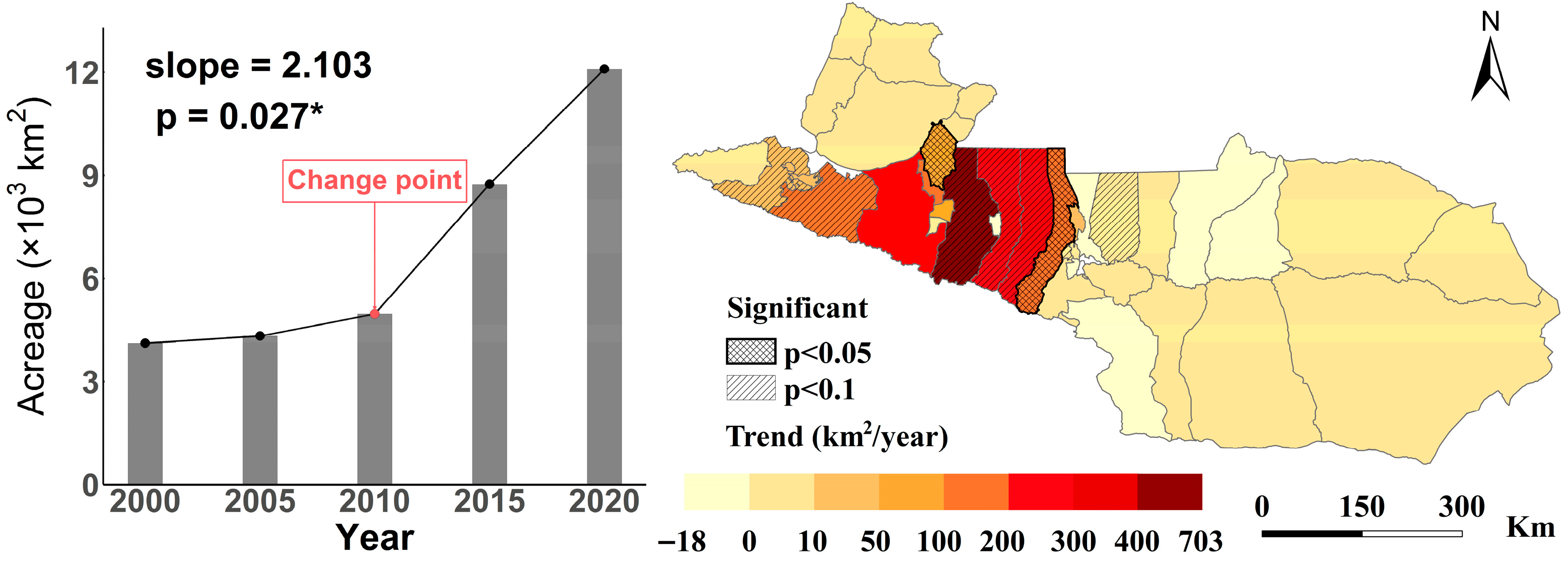
The cotton area has undergone substantial expansion, with an average annual growth rate of 2.10 × 10³ km²/year in the past two decades in the NSTM (based on data from 2000, 2005, 2010, 2015, and 2020). It is notable that an abrupt change point occurred in 2000, found by a moving t-test. The growth rates before and after this turning point were significantly different, with 0.43 × 10³ km²/year and 3.57 × 10³ km²/year, respectively. The area of cotton cultivation in the northwest and central regions of the NSTM has increased dramatically from 2000 to 2020, with growth rates of 176 and 142 km²/year, respectively. Additionally, the expansion of cotton cultivation in the western regions, such as the Bortala Mongol Autonomous Prefecture and certain directly administered municipalities, cannot be ignored either.

Further county-by-county analysis was conducted to examine the temporal change patterns of cotton cultivation using Theil–Sen median combined with MK (Figure 4). The counties in the central and western parts of the study area are the primary cotton-growing regions of the NSTM. Among these, 83.78% of the counties show an increase in cotton-planting area over the past 20 years, with a significant increase in 29.03% (p < 0.1) of these counties.

3.2.2. Spatial Variations in Cotton Cultivation

The global Moran’s I and the local spatial association index of Getis-Ord $G_i^{*}$ were used to analyze the evolution of the spatial patterns of cotton cultivation on the NSTM. The global Moran’s I indices for the years 2000, 2005, 2010, 2015, and 2020 were 0.369, 0.331, 0.420, 0.374, and 0.368, respectively. The Z-scores for each year all exceeded the critical value of 2.58 and passed the significance level test of 0.01. It is shown that the cotton distribution of the NSTM has a significant and positive spatial autocorrelation in the global region. Moreover, the spatial associations present the weakening–strengthening–weakening trend, indicating the overall spatial distribution pattern of high–high and low–low agglomeration.

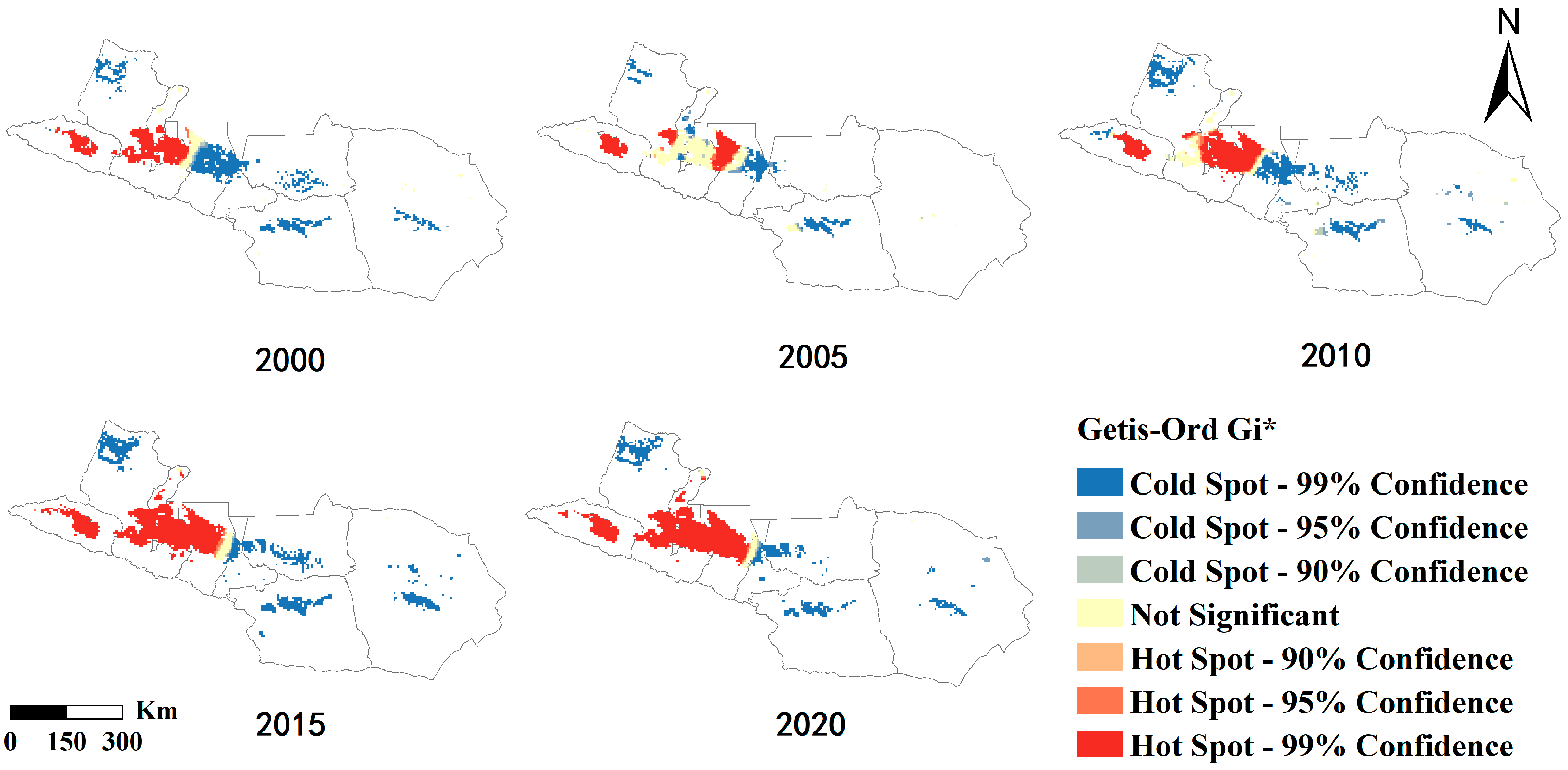
Cold–hot analysis can indicate high-value cluster areas and low-value cluster areas of relevant variables in different districts. The distribution of cold spots in the NSTM were relatively scattered but showed differences over time (Figure 5). The low values of the cotton area were basically significant at the 99% confidence level, mainly situated in the northwest, middle, and east of this region. Except for 2005, the spatial distribution patterns of cotton cold spots were relatively consistent, predominantly extending from the northwest directly to the central-eastern region, while the scope of cold spots was smaller in 2005. The distribution patterns of cotton hot spots in various years were similar, basically extending from the west to the middle of the study area. The scope of hot spots increased and expanded spatially from 2010 to 2020. However, hot spot areas were the smallest in 2005.

3.3. Drivers of Spatiotemporal Patterns for Cotton and Contributions of Relevant Factors

3.3.1. Impacts of Factors on Cotton Cultivation at the Global Scale

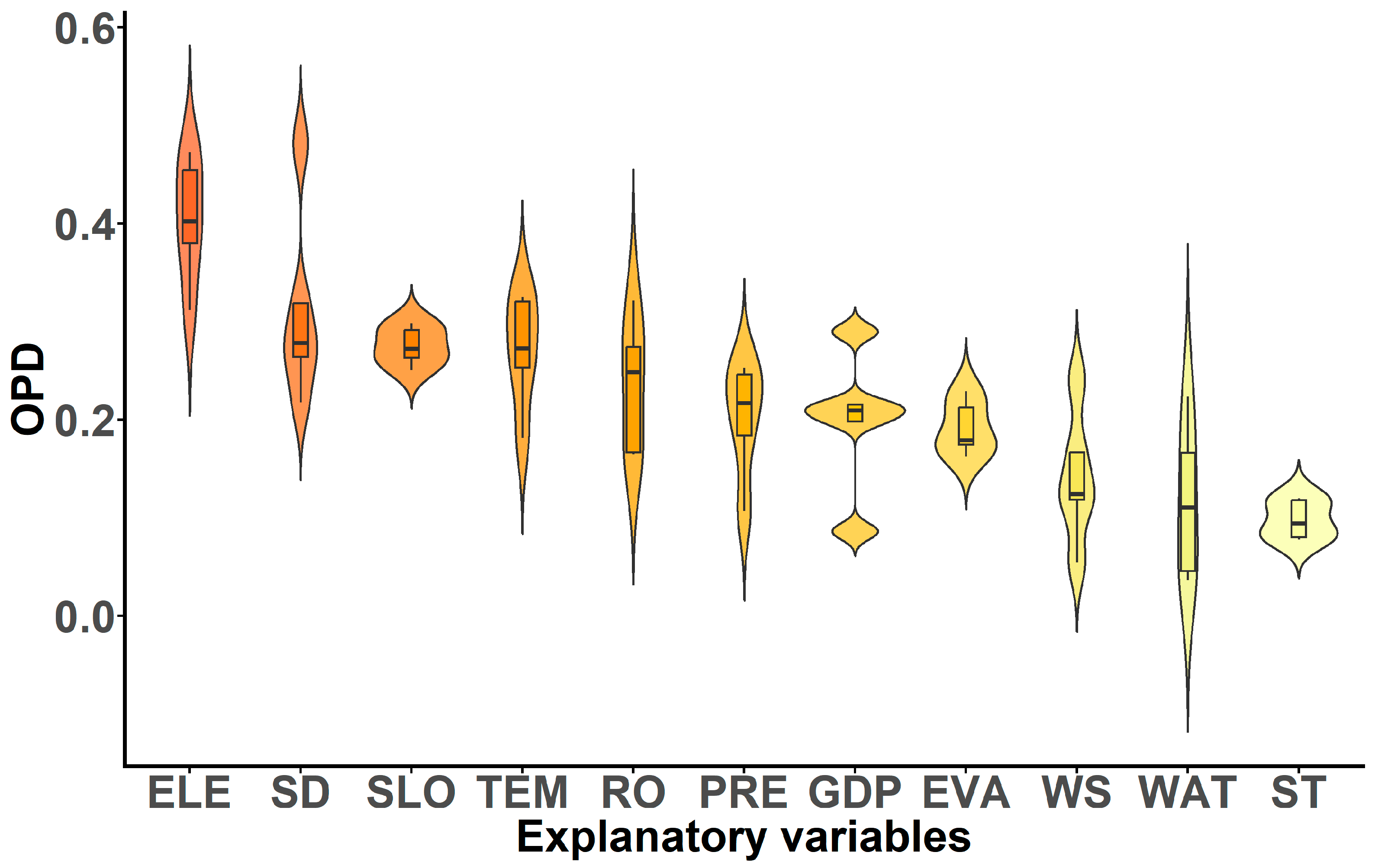
This study used the LESH model to analyze the explanatory power of 11 factors on the spatiotemporal changes in cotton in the global region (Figure 6 and Figure 7). Figure 6 shows the OPD values of different factors at the scale of 17 km over 20 years. It can be observed that topographic factors have the highest spatial associations with cotton area, followed by climatic and water-resource factors. Notably, the ELE has the highest average OPD value among the eleven factors, explaining 40% of the spatial heterogeneity of the cotton distribution on average. However, there are certain differences in its OPD values for each year. This OPD rose by 7.45% over 20 years. Compared with those of other factors, the OPD values of ELE in 2000 and 2005 ranked second, while its OPD value increased from 2010 to 2020 and remained first. The ELE variable has the most explanatory power over the spatial variability of cotton and is the primary condition for the expansion of cotton cultivation. Furthermore, the SLO from topographic variables is one of the stable conditions influencing cotton distributions on the NSTM, with its average OPD value of 0.28 ranking third and the standard deviation of OPD value for 0.02 being the lowest among all factors.

Among the climatic variables, the SD factor has an average OPD value of 0.31, ranking second among all explanatory variables, but has the highest standard deviation of OPD value over 20 years. Its OPD value decreased by 26.38% over 20 years. It is demonstrated that the explanatory power of the SD had been weakening over 20 years. In addition, the TEM also plays a significant role in explaining the spatial variability of cotton cultivation in the study area, with a mean OPD value of 0.27. The OPD value had been rising and increased by 7.19% over 20 years. Two factors, RO and PRE, exhibited moderate explanatory power over the spatial heterogeneity of the cotton spatiotemporal distribution in the NSTM, with OPD values of 0.23 and 0.20, respectively. The moderate OPD levels of these two factors indicate that both RO and PRE played a secondary but non-negligible role in shaping the spatial patterns of cotton planting, particularly in areas with varying water availability. Moreover, it is noteworthy that the OPD values of the GDP factor exhibited an increasing trend over time, although its mean OPD value was only 0.20, rising by 20.35% over 20 years. This reveals the important impact of socio-economic factors on cotton distribution. The remaining factors, including EVA, WS, WAT, and ST, had relatively smaller influence on cotton distribution in the NSTM, with OPD values all below 0.20. This indicates that, compared with the more dominant topographic and climatic drivers, these factors played a minor role in shaping the spatial patterns of cotton cultivation and can be considered as supplementary reference factors.

3.3.2. Impacts of the Interactions Between Pairwise Factors

The geographical system is complex, owing to the coexistence of impacts from individual factors and the interactions of multiple factors. This study quantified the interactive effects between two factors and revealed the contribution of each factor to the interaction (Figure 7). The results show that the interactions between topographic variables and other variables had the strongest explanatory power for the distribution of cotton planting, especially the ELE in topographic variables. The OPD values of the interactions between ELE and other variables were almost all higher than 0.4, in various years. Climatic variables and socio-economic variables had the second strongest explanatory power for cotton distribution. Among the interactions involving non-topographic variables, the interaction effect between the SD and the GDP had the greatest impact on the spatial variability of cotton cultivation, with OPD values ranging from 0.40 to 0.56 over 20 years.

Furthermore, nonlinear weakening interactions between two factors were detected, as evidenced by the interactive OPD value being lower than the sum of the individual OPD values of the two variables, yet higher than the OPD value of either variable. For instance, the interactions between TEM and other variables exhibited the nonlinear weakening effect. In 2020, the interactive OPD value between TEM and RO was 0.48, while the individual OPD values of TEM and RO were 0.33 and 0.25, respectively. Moreover, it is found that this factor plays the dominant role in the interaction if the independent explanation of a factor is high. For the above interaction between TEM and RO, their SPD values were 0.28 and 0.20, respectively.

3.3.3. Key Factors Dominating Local Spatial Heterogeneity

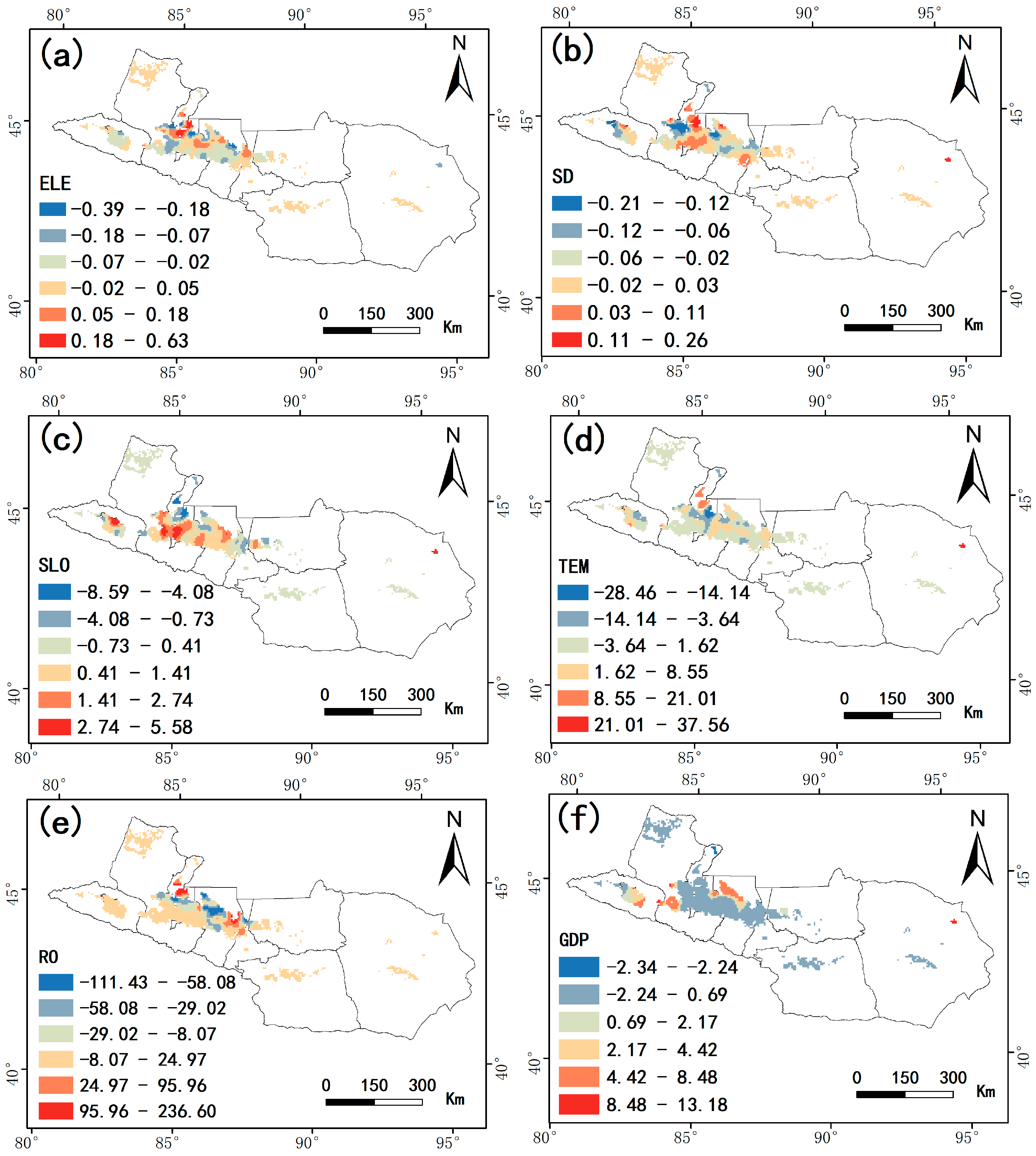
The GWR model was further introduced to conduct local spatial regression analysis for exploring the direction and intensity of the six global dominant factors in the local regions, with the factors of ELE, SD, SLO, TEM, RO, and GDP. The GWR models in various years showed higher fitness with the adjusted R² values ranging from 0.75 to 0.86. Meanwhile, it can be observed that these six factors all had spatial non-stationarity through the collinearity diagnosis based on the variance inflation factor.

In addition, these factors exhibited different characteristics of spatial variability in the local areas, according to the regression coefficients of the factors in the models (Figure 8). The impacts of ELE on the local variability of cotton distribution showed less fluctuation compared to those of the other five explanatory variables, according to the smaller regression coefficients of this variable, ranging from 0.04 to 0.09 across various years. Its influence on cotton distribution was negative in approximately 70% of the cotton area, mainly concentrated in the city of Karamay, adjacent to the western side of the Junggar Basin. The spatial non-stationarity of the SD is slightly greater than that of ELE, with its regression coefficients varying markedly across different regions from 2000 to 2015. On the whole, the positive effects of SD outweighed its negative effects. However, its synergistic stress with high temperature or drought should be paid more attention. The SLO had greater local influential power on cotton distribution and mainly positive effects, with a regression coefficient between −8.59 and 5.58. The average slope value in the cotton planting area is less than 5°, generally belonging to the category of gentle-slope land and highly suitable for cotton cultivation. For the TEM, the local impact on cotton distribution was relatively weak because of the fewer areas with high values of the regression coefficient. RO had greater spatial non-stationarity, with high values and standard deviation of the regression coefficient in comparison to other factors. The areas with a stronger effect are mainly located in the west of the Changji Hui Autonomous Prefecture and Karamay City. Finally, it can be observed that spatial differences in impacts of the GDP are also not ignored. The effect is predominantly positive, with approximately 67% of the analysis units exhibiting a regression coefficient greater than zero. Areas with dominant influence are primarily concentrated in the central and western regions of the Bortala Mongolian Autonomous Prefecture, the central and southern parts of the Tacheng Prefecture, and the northwestern area of the Changji Hui Autonomous Prefecture.

4. Discussion

4.1. Spatial Scale Effects on Exploring for Drivers of Cotton Spatiotemporal Patterns

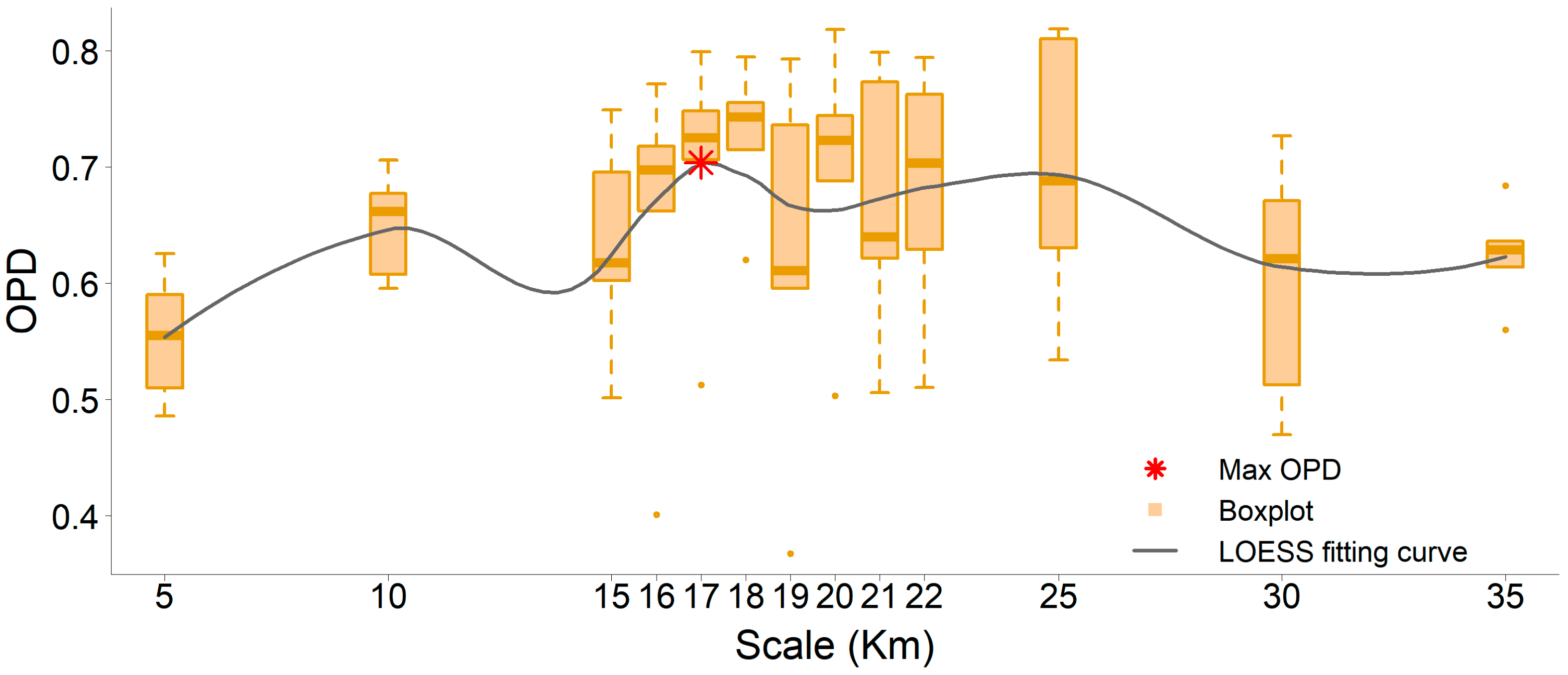
Understanding and simulating scale effects is a prerequisite for accurately analyzing spatial patterns and geographic processes. The size of spatial scales presents the balance between the granularity of the study and the strength of interpretation. The choice of finer scales brings an increase in data volume, computational demands, and analytical complexity, although there is more detailed information at a finer scale. Conversely, for the coarser scales, the manifestation of spatial characteristics for geographic variables is limited [47,48]. The scale effects are the fact that the statistical indicators of variables and multi-attribute correlations change with scales. Therefore, this study employed the LESH model to calculate the average OPD value of 11 explanatory variables in order to analyze the comprehensive impacts of these variables on cotton spatiotemporal patterns at different scales and identify the optimal scale for the spatial heterogeneity of cotton distribution (Figure 9). It can be observed that the OPD value changed in accordance with spatial scales in a fluctuating manner, with rising–decreasing values based on the fitting of the locally estimated scatterplot smoothing model. The highest value was reached at the 17 km scale. Therefore, we chose 17 km as the optimal scale for analysis.

4.2. Interpretations of Driving Forces of Cotton Spatiotemporal Variability

The formation of the spatiotemporal patterns for cotton cultivation is the result of the combining effect of internal and external factors. The analysis of driving forces of cotton spatiotemporal variability from the perspective of spatial heterogeneity and dependence can provide important support for optimizing crop planting and improving resource utilization efficiency. This study proposed the combination of the LESH and GWR models to explore the global and local influential strength of various kinds of factors impacting the spatiotemporal patterns of cotton in the NSTM. The global dominant factors influencing the spatiotemporal variability of cotton cultivation patterns from 2000 to 2020 were identified as ELE, SD, SLO, TEM, RO, and GDP. To some extent, this result is consistent with previous studies [49,50]. For example, Zhu et al. [51] identified geographic region and temperature as primary drivers using the geographical detector, which aligns with our findings. However, this study did not provide local-scale descriptions or clearly quantify the contributions of interacting factors, although it did assess factor importance at the global scale. It is found that ELE is the primary driver of cotton distribution. This is because climatic conditions are different at various altitudes, directly affecting the suitability of the area for cotton cultivation and yield. About 95% of cotton areas in the NSTM are situated at low altitudes. However, with the expansion of the cotton planting area, the potential for cotton cultivation in the middle-altitude marginal has been increasing since 2015. This is attributed to global warming and the optimization of varieties and agricultural technologies. Additionally, this study also detected local positive effects of elevation on cotton-planting patterns and the influence of strong interactions between this factor and other factors. The SD in climatic variables is the second explanatory power of cotton-planting patterns. Sufficient sunlight is one of the key factors for high yield and quality of cotton, while insufficient sunlight affects the photosynthesis and dry matter accumulation of cotton. Over the past few decades, temperature and sunshine duration in the north of Xinjiang have been on an upward trend [52]. The nonlinear interaction between SD and TEM in the NSTM is relatively strong, which can lead to an earlier start of the cotton sowing time and a later end of the dormancy time, namely an overall extension of the growing period in the field. However, we found that the explanatory power of the SD on cotton distribution had been weakening from 2000 to 2020. This may be related to improvements in modern cultivated varieties, reducing cotton’s sensitivity to sunshine.

RO, PRE and GDP are three variables with moderate explanatory power for the evolution of cotton spatiotemporal patterns. The long-term change trend of RO in the NSTM was not significant over the 20 years, while the cycle fluctuation was obvious, with the distribution of low in the northwest and high in the southeast. This did not correspond to the distribution of irrigation water demand during the entire growth period of cotton [53]. Therefore, the global and local influences of RO and its interactions with TEM or the SD are the important considerations in the optimization of cotton planting scale and distribution. Furthermore, GDP is an influencing factor that cannot be ignored in the evolution of cotton-planting patterns in the NSTM. Since 2000, the GDP in the study area has been trending upward and increasing in explanatory power over cotton distribution, according to the increased OPD values obtained by the LESH model, with particularly significant positive effects in the local districts. When the GDP increases, subsidies and technological investments rise. Mechanization can be easily adopted in the study area with gentle slopes, indicating that the newly formed cotton land has spatial associations with the socio-economic variables.

The LESH model explores interactions among multiple factors at the global scale and quantifies the contributions of individual factors, while the GWR model captures local variations by allowing regression coefficients to vary across geographic locations. By combining LESH and GWR, this study provides a more detailed and interpretable assessment of the spatiotemporal evolution of cotton-planting patterns in the NSTM over the past 20 years, from both global and local perspectives. Despite this, the study chose to observe fewer human factors that affect the cotton planting distribution, such as market supply, policy and regulations, technological innovation, and other explanatory factors. Cotton, as a globally significant economic crop, exhibits production fluctuations influenced not only by natural factors but also by anthropogenic drivers such as technology adoption and cotton price volatility, which can induce variations in its cultivation patterns across different years. However, the fine-scale spatial quantification of these factors remains a substantial challenge. Furthermore, the weakening nonlinear interaction between the variables detected by this study indicates partial synergy between variables, but the combined effect does not achieve a full linear superposition. Such behavior may arise from partial redundancy, mutual inhibition, or shared dependence on an underlying latent mechanism. Quantifying this latent mechanism is critical for providing more precise guidance in optimizing cotton planting.

5. Conclusions

This study proposed the combination of the LESH and GWR models to reveal the drivers of the spatiotemporal distribution of cotton in the NSTM from 2000 to 2020 from the perspective of spatial heterogeneity. First of all, we generated the cotton planting distribution in the NSTM from 2000 to 2020 using the long time series images of Landsat on the GEE platform. The area of cotton planting in the study area has increased rapidly, with an average annual growth rate of 2.10 × 10³ km²/year. The counties in the central and western parts of the NSTM were the main cotton-planting areas. The cotton distribution exhibited the pattern of high–high and low–low agglomeration in the NSTM. Cold spot areas of cotton were primarily concentrated in the northwestern and central-eastern parts of this region, while hot spot areas generally extended from the western region toward the central part of the study area over the 20 observed years.

Based on the spatiotemporal evolution and regional differentiation characteristics of cotton planting, it is found that the dominant factors explaining the spatiotemporal patterns of cotton are the ELE, SD, SLO, TEM, RO, and GDP, according to the LESH and GWR models over the 20 years observed in the NSTM. Moreover, these factors exhibit different spatial effects on cotton distribution in the local areas over the 20 years. The average OPD value of ELE is the highest, explaining the average 40% spatial heterogeneity of the cotton spatiotemporal distribution. The explanatory power of the SD from climate variables ranked second and had weakened over the 20 years. The SLO is one of the stable factors affecting cotton distribution, with similar OPD values across different years. The explanatory power of TEM showed an upward trend over the 20 years. The three factors of RO, PRE, and GDP exhibited moderate explanatory power over the spatial heterogeneity of cotton spatiotemporal distribution in the NSTM. It is noteworthy that the mean OPD value of the GDP was relatively low from 2000 to 2020 but increased progressively over time.

In addition to examining the impacts of individual factors, this study quantitatively evaluated the influence of interactions between two variables on the evolution of cotton spatiotemporal patterns. The interactions between ELE and other variables demonstrated the primary explanatory power over cotton distribution, followed by those between climatic and socio-economic variables. Notably, the interactions between the GDP and other variables intensified with the increase in the GDP in the NSTM over the 20 years. This indicates that the consideration of their synergistic interactions is essential for optimization of cotton planting distribution, particularly the underlying mechanisms of mutual inhibition or interdependence between these factors.

References

1. USDA. Available online: https://apps.fas.usda.gov/psdonline/circulars/cotton.pdf (accessed on 3 March 2025).
2. Wang, Y.; Peng, S.; Huang, J.; Zhang, Y.; Feng, L.; Zhao, W.; Qi, H.; Zhou, G.; Deng, N. Prospects for Cotton Self-Sufficiency in China by Closing Yield Gaps. Eur. J. Agron. 2022, 133, 126437. [Google Scholar] [CrossRef]
3. Zhang, X.; Zhou, X.; Liu, H.; Zhang, J.; Zhang, J.; Wei, S. The Impact of Factor Price Change on China’s Cotton Production Pattern Evolution: Mediation and Spillover Effects. Agriculture 2024, 14, 1145. [Google Scholar] [CrossRef]
4. Jiang, S.; Yu, J.; Li, S.; Liu, J.; Yang, G.; Wang, G.; Wang, J.; Song, N. Evolution of Crop Planting Structure in Traditional Agricultural Areas and Its Influence Factors: A Case Study in Alar Reclamation. Agronomy 2024, 14, 580. [Google Scholar] [CrossRef]
5. Li, P.; He, Z.; He, D.; Xue, D.; Wang, Y.; Cao, S. Fractional Vegetation Coverage Response to Climatic Factors Based on Grey Relational Analysis during the 2000–2017 Growing Season in Sichuan Province, China. Int. J. Remote Sens. 2020, 41, 1170–1190. [Google Scholar] [CrossRef]
6. Gong, Y.; Li, J.; Li, Y. Spatiotemporal Characteristics and Driving Mechanisms of Arable Land in the Beijing-Tianjin-Hebei Region during 1990–2015. Socio-Econ. Plan. Sci. 2020, 70, 100720. [Google Scholar] [CrossRef]
7. Lundberg, S.M.; Erion, G.; Chen, H.; DeGrave, A.; Prutkin, J.M.; Nair, B.; Katz, R.; Himmelfarb, J.; Bansal, N.; Lee, S.-I. From Local Explanations to Global Understanding with Explainable AI for Trees. Nat. Mach. Intell. 2020, 2, 56–67. [Google Scholar] [CrossRef]
8. Elhorst, J.P. Matlab Software for Spatial Panels. Int. Reg. Sci. Rev. 2014, 37, 389–405. [Google Scholar] [CrossRef]
9. Brunsdon, C.; Fotheringham, A.S.; Charlton, M.E. Geographically Weighted Regression: A Method for Exploring Spatial Nonstationarity. Geogr. Anal. 1996, 28, 281–298. [Google Scholar] [CrossRef]
10. Song, Y.; Wang, J.; Ge, Y.; Xu, C. An Optimal Parameters-Based Geographical Detector Model Enhances Geographic Characteristics of Explanatory Variables for Spatial Heterogeneity Analysis: Cases with Different Types of Spatial Data. GISci. Remote Sens. 2020, 57, 593–610. [Google Scholar] [CrossRef]
11. Luo, P.; Song, Y.; Huang, X.; Ma, H.; Liu, J.; Yao, Y.; Meng, L. Identifying Determinants of Spatio-Temporal Disparities in Soil Moisture of the Northern Hemisphere Using a Geographically Optimal Zones-Based Heterogeneity Model. ISPRS J. Photogramm. Remote Sens. 2022, 185, 111–128. [Google Scholar] [CrossRef]
12. Shapley, L.S. A Value for N-Person Games; RAND Corporation: Santa Monica, CA, USA, 1952; p. 295. [Google Scholar]
13. Li, Y.; Luo, P.; Song, Y.; Zhang, L.; Qu, Y.; Hou, Z. A Locally Explained Heterogeneity Model for Examining Wetland Disparity. Int. J. Digit. Earth 2023, 16, 4533–4552. [Google Scholar] [CrossRef]
14. Zhang, K.; Wang, Y.; Mamtimin, A.; Liu, Y.; Zhang, L.; Gao, J.; Aihaiti, A.; Wen, C.; Song, M.; Yang, F.; et al. Simulation and Attribution Analysis of Spatial–Temporal Variation in Carbon Storage in the Northern Slope Economic Belt of Tianshan Mountains, China. Land 2024, 13, 608. [Google Scholar] [CrossRef]
15. Wang, K.; Ma, H.; Fang, C. The Relationship Evolution between Urbanization and Urban Ecological Resilience in the Northern Slope Economic Belt of Tianshan Mountains, China. Sustain. Cities Soc. 2023, 97, 104783. [Google Scholar] [CrossRef]
16. Sun, Y.; Liu, B.; Yang, G.; Du, Y.; Huang, H.; Wang, T.; Wang, J. Analysis of Spatiotemporal Evolution Patterns and Driving Forces of Reservoirs on the Northern Slope of the Tianshan Mountains in Xinjiang. Sustainability 2023, 15, 8824. [Google Scholar] [CrossRef]
17. Zhu, C.; Fang, C.; Zhang, L. Analysis of the Coupling Coordinated Development of the Population–Water–Ecology–Economy System in Urban Agglomerations and Obstacle Factors Discrimination: A Case Study of the Tianshan North Slope Urban Agglomeration, China. Sustain. Cities Soc. 2023, 90, 104359. [Google Scholar] [CrossRef]
18. Yang, Z.; Zhang, S.; Lei, J.; Zhang, X.; Tong, Y.; Duan, Z.; Fan, L. Evolution of Economic Linkage Network of the Cities and Counties on the Northern Slope of the Tianshan Mountains, China. Reg. Sustain. 2023, 4, 173–184. [Google Scholar] [CrossRef]
19. Xinjiang Scientific Expedition Data Sharing Service Platform. Available online: https://cstr.cn/CSTR:33110.11.XIEG.xjsedata.2022.00000095 (accessed on 10 May 2024).
20. Geospatial Data Cloud. Available online: http://www.gscloud.cn (accessed on 6 March 2025).
21. Copernicus Climate Data Store. Available online: https://cds.climate.copernicus.eu (accessed on 6 March 2025).
22. Sun, W.; Shao, Q.; Liu, J.; Zhai, J. Assessing the Effects of Land Use and Topography on Soil Erosion on the Loess Plateau in China. CATENA 2014, 121, 151–163. [Google Scholar] [CrossRef]
23. Sun, W.; Song, X.; Mu, X.; Gao, P.; Wang, F.; Zhao, G. Spatiotemporal Vegetation Cover Variations Associated with Climate Change and Ecological Restoration in the Loess Plateau. Agr. For. Meteorol. 2015, 209–210, 87–99. [Google Scholar] [CrossRef]
24. Sun, W.; Mu, X.; Song, X.; Wu, D.; Cheng, A.; Qiu, B. Changes in Extreme Temperature and Precipitation Events in the Loess Plateau (China) during 1960–2013 under Global Warming. Atmos. Res. 2016, 168, 33–48. [Google Scholar] [CrossRef]
25. Zhang, Z.; Fang, S.; Han, J. A Daily Sunshine Duration (SD) Dataset in China from Himawari AHI Imagery (2016–2023). Earth Syst. Sci. Data 2025, 17, 1427–1439. [Google Scholar] [CrossRef]
26. Resource and Environmental Science Data Platform. Available online: https://www.resdc.cn/ (accessed on 6 March 2025).
27. Data Sharing and Service Portal. Available online: https://data.casearth.cn/ (accessed on 6 March 2025).
28. Agarwal, S.C. Gross Domestic Product & it’s Various Approaches. Int. J. Tax Econ. Manag. 2018, 1, 70–85. [Google Scholar] [CrossRef]
29. Xinjiang Uygur Autonomous Region Platform for Common Geospatial Information Services. Available online: https://xinjiang.tianditu.gov.cn/ (accessed on 6 March 2025).
30. Xinjiang Scientific Expedition Data Sharing Service Platform. Available online: https://cstr.cn/CSTR:33110.11.XIEG.xjsedata.2022.00009105 (accessed on 10 May 2024).
31. Ok, A.O.; Akar, O.; Gungor, O. Evaluation of Random Forest Method for Agricultural Crop Classification. Eur. J. Remote Sens. 2012, 45, 421–432. [Google Scholar] [CrossRef]
32. NASA Shuttle Radar Topography Mission Global 1 arc Second V003 | NASA Earthdata. Available online: https://www.earthdata.nasa.gov/data/catalog/lpcloud-srtmgl1-003 (accessed on 10 May 2024).
33. Metternicht, G. Vegetation Indices Derived from High-Resolution Airborne Videography for Precision Crop Management. Int. J. Remote Sens. 2003, 24, 2855–2877. [Google Scholar] [CrossRef]
34. Broge, N.H.; Leblanc, E. Comparing Prediction Power and Stability of Broadband and Hyperspectral Vegetation Indices for Estimation of Green Leaf Area Index and Canopy Chlorophyll Density. Remote Sens. Environ. 2001, 76, 156–172. [Google Scholar] [CrossRef]
35. Huete, A.; Justice, C.; Liu, H. Development of Vegetation and Soil Indices for MODIS-EOS. Remote Sens. Environ. 1994, 49, 224–234. [Google Scholar] [CrossRef]
36. Roujean, J.-L.; Breon, F.-M. Estimating PAR Absorbed by Vegetation from Bidirectional Reflectance Measurements. Remote Sens. Environ. 1995, 51, 375–384. [Google Scholar] [CrossRef]
37. Steven, M.D. The Sensitivity of the OSAVI Vegetation Index to Observational Parameters. Remote Sens. Environ. 1998, 63, 49–60. [Google Scholar] [CrossRef]
38. Ye, B.; Yu, R.; Gao, A.; Bai, Y.; Yu, G. Interannual Dynamics and Driving Mechanisms of the Shrinkage for Lake Groups in the Jiziwan Region of Yellow River from 1986 to 2024. J. Hydrol. Reg. Stud. 2025, 61, 102752. [Google Scholar] [CrossRef]
39. Sen, P.K. Estimates of the Regression Coefficient Based on Kendall’s Tau. J. Am. Stat. Assoc. 1968, 63, 1379–1389. [Google Scholar] [CrossRef]
40. Gao, Z.; Ju, X.; Ding, J.; Wang, Y.; Shen, N.; Zhang, X.; Li, M. Understanding Water Yield Dynamics and Drivers in the Yellow River Basin Past Trends, Mechanisms, and Future Projections. J. Clean. Prod. 2025, 505, 145441. [Google Scholar] [CrossRef]
41. Wang, M.; Chen, Y.; Li, J.; Zhao, Y. Spatiotemporal Evolution and Driving Force Analysis of Drought Characteristics in the Yellow River Basin. Ecol. Indic. 2025, 170, 113007. [Google Scholar] [CrossRef]
42. Chen, Y.; Shu, B.; Amani-Beni, M.; Wei, D. Spatial Distribution Patterns of Rural Settlements in the Multi-Ethnic Gathering Areas, Southwest China: Ethnic Inter-Embeddedness Perspective. J. Asian Archit. Build. Eng. 2024, 23, 372–385. [Google Scholar] [CrossRef]
43. Guerri, G.; Crisci, A.; Congedo, L.; Munafò, M.; Morabito, M. A Functional Seasonal Thermal Hot-Spot Classification: Focus on Industrial Sites. Sci. Total Environ. 2022, 806, 151383. [Google Scholar] [CrossRef]
44. Zhang, L.; Wang, P.; Xie, G.; Wang, W. Spatial Distribution Pattern of Aromia Bungii Within China and Its Potential Distribution Under Climate Change and Human Activity. Ecol. Evol. 2024, 14, e70520. [Google Scholar] [CrossRef]
45. Wang, J.; Li, X.; Christakos, G.; Liao, Y.; Zhang, T.; Gu, X.; Zheng, X. Geographical Detectors-Based Health Risk Assessment and Its Application in the Neural Tube Defects Study of the Heshun Region, China. Int. J. Geogr. Inf. Sci. 2010, 24, 107–127. [Google Scholar] [CrossRef]
46. Guo, H.; Tang, Y.; Guo, J. Spatial Heterogeneity of Traditional Villages in Southern Sichuan, China: Insights from GWR and K-Means Clustering. Land 2025, 14, 1817. [Google Scholar] [CrossRef]
47. Wang, Y.; Di, Q. Modifiable Areal Unit Problem and Environmental Factors of COVID-19 Outbreak. Sci. Total Environ. 2020, 740, 139984. [Google Scholar] [CrossRef] [PubMed]
48. Lin, Y.; Xu, X.; Tan, Y.; Chen, M. Multi-Scalar Assessment of Ecosystem-Services Supply and Demand for Establishing Ecological Management Zoning. Appl. Geogr. 2024, 172, 103435. [Google Scholar] [CrossRef]
49. Zhang, H.; Zhu, Y.; Ma, Z.; He, J.; Guo, C.; Zhou, Q.; Song, L. Simulating the Impact of Climate Change on the Suitable Area for Cotton in Xinjiang Based on SDMs Model. Ind. Crops Prod. 2025, 227, 120750. [Google Scholar] [CrossRef]
50. Li, N.; Lin, H.; Wang, T.; Li, Y.; Liu, Y.; Chen, X.; Hu, X. Impact of Climate Change on Cotton Growth and Yields in Xinjiang, China. Field Crops Res. 2020, 247, 107590. [Google Scholar] [CrossRef]
51. Zhu, Y.; Zheng, B.; Luo, Q.; Jiao, W.; Yang, Y. Uncovering the Drivers and Regional Variability of Cotton Yield in China. Agriculture 2023, 13, 2132. [Google Scholar] [CrossRef]
52. Zhu, Y.; Sun, L.; Luo, Q.; Chen, H.; Yang, Y. Spatial Optimization of Cotton Cultivation in Xinjiang: A Climate Change Perspective. Int. J. Appl. Earth Obs. Geoinf. 2023, 124, 103523. [Google Scholar] [CrossRef]
53. Geng, Q.; Zhao, Y.; Sun, S.; He, X.; Wang, D.; Wu, D.; Tian, Z. Spatio-Temporal Changes and Its Driving Forces of Irrigation Water Requirements for Cotton in Xinjiang, China. Agric. Water Manag. 2023, 280, 108218. [Google Scholar] [CrossRef]
Figure 1. Study area location.
Agriculture 15 02163 g001
Figure 2. Cotton, maize, and wheat growth calendar.
Agriculture 15 02163 g002
Figure 3. Distribution of sample sites in 2020.
Agriculture 15 02163 g003
Figure 4. Trend of cotton-planting area from 2000 to 2020. * indicates p < 0.05.
Agriculture 15 02163 g004
Figure 5. Distribution of cotton cold–hot spots from 2000 to 2020.
Agriculture 15 02163 g005
Figure 6. Variation in OPD values of different factors at the 17 km scale (2000–2020).
Agriculture 15 02163 g006
Figure 7. Quantification of the interactive effects and contributions of paired factors. (a) Year 2000; (b) Year 2005; (c) Year 2010; (d) Year 2015; and (e) Year 2020.
Agriculture 15 02163 g007
Figure 8. Spatial distribution of GWR coefficients for key explanatory variables: (a) ELE; (b) SD; (c) SLO; (d) TEM; (e) RO; and (f) GDP.
Agriculture 15 02163 g008
Figure 9. Optimal research scale.
Agriculture 15 02163 g009