Article

On Improving the Performance of Kalman Filter in Denoising Oil Palm Hyperspectral Data

by
Imanurfatiehah Ibrahim
1,
Hamzah Arof
1,*,
Mohd Izzuddin Anuar
2 and
Mohamad Sofian Abu Talip
1
1
Department of Electrical Engineering, Faculty of Engineering, Universiti Malaya, Kuala Lumpur 50603, Malaysia
2
Malaysian Palm Oil Board (MPOB), No. 6, Persiaran Institusi, Bandar Baru Bangi, Kajang 43000, Malaysia
*
Author to whom correspondence should be addressed.
Agriculture 2025, 15(20), 2149; https://doi.org/10.3390/agriculture15202149 (registering DOI)
Submission received: 15 August 2025 / Revised: 12 October 2025 / Accepted: 13 October 2025 / Published: 15 October 2025
(This article belongs to the Section Artificial Intelligence and Digital Agriculture)

Abstract

A common drawback of denoising methods of images is that all pixels are filtered regardless of the amount of noise affecting them individually. Since the essence of denoising is lowpass filtering, subjecting clean pixels to denoising results in blurring. In this paper, a filtering framework is introduced where a fitness function is incorporated in a Kalman filter (KF) to assess the suitability of accepting the value recommended by KF or retaining the existing value of a pixel. Furthermore, a limit on the number of iterations is imposed to avoid over filtering that leads to shrinkage of pixel value ranges of the channels and loss of spectral signatures. In post processing, the means of the filtered channels are shifted to their original values prior to filtering, to spread the pixel value ranges and regain important spectral signatures. The experiments involve the implementation of KF, extended Kalman filter (EKF), Kalman smoother (KS), extended Kalman smoother (EKS) and moving average filter (MAF) in filtering noisy channels of oil palm hyperspectral data under the same framework. Their performances are compared in terms of execution time, SNR gain, NIQE and SSIM metrics. In the second set of experiments, the performance of the improved KF with a fitness function and mean restoration is compared to those of KF and MAF. The results show that the improved KF outperforms the other two filters in the spectral signature characteristics and pixel value ranges of the denoised channels.

1. Introduction

Often, hyperspectral data of oil palms acquired from UAVs contain noise caused by various factors. Speckle noise that appears as white and black specks degrades the quality of the bands [1]. It obscures important features in the channels and hinders their extraction. Without effective filtering, some noisy channels are thrown away as the information in them is deemed irrecoverable. This is a common practice adopted by researchers who process hyperspectral data, as part of the process of band selection [2]. Furthermore, noise may alter the spectral signatures of the data, making them different from those of field spectroscopy of similar wavelengths taken on the ground [1]. However, those noisy channels may still contain important information that is not available in others. This is especially true for channels of long and short wavelengths since they suffer higher noise degradation than the medium wavelength bands.
Since the channels are captured simultaneously using bands of wavelengths that are very close together, a high spectral correlation among neighboring bands is expected. However, it is also known that some channels contain exclusive information that is not available in others. When combined, the information on different channels complement each other. While filtering is necessary for removing noise, it also alters the content of the channels inadvertently. Thus, filtering should be implemented sparingly to preserve the important spectral signatures of the channels.
This paper presents a framework to denoise oil palm hyperspectral data from speckle noise using KF, EKF, KS and EKS. There are three steps in the framework, and they are noisy channel selection, spectral and spatial filtering, and channel mean restoration. KF, EKF, KS and EKS are used in the spectral and spatial filtering as they are good at estimating the values of the pixels in the presence of noise. After denoising, SNR gain, execution time, NIQE and SSIM indices are calculated to gauge the improvement made for the filtered channels. Then, the performance of KF is improved by introducing a local fitness function that assesses whether the value of a pixel should be replaced by the one produced by Kalman filter. The local fitness function is the inverse of the sum of the absolute difference between the center pixel and its nearest neighbors. A limit on the number of filtering iterations is also imposed to avoid over filtering. Finally, in post processing, the bunching of pixel value ranges of neighboring channels is mitigated by restoring the means of the filtered channels to their original values to regain some the spectral undulations of the raw data.

2. Literature Review

Many denoising approaches have been introduced to filter noise in hyperspectral data. Some are straightforward to implement, while others require intensive training and many iterations. There are two main strategies of denoising hyperspectral data, and they are the spatial–spectral and the deep learning neural network approaches. In essence, both methods seek to reduce local variations or increase likeness in similar areas by adjustment or replacement of pixel values. The effect is akin to lowpass filtering the target areas. Spatial spectral approaches make use of spectral correlation, sparsity promotion, variation minimization, selective data content reduction, low-rank matrix or tensors and lowpass filtering to reduce volatility manifested by noise in the channels. Deep learning methods train the neural networks to generate a clean output given a noisy input. They need extensive training to establish numerous parameter values that are stored in the form of matrices. Therefore, they require a lot of noisy and clean data in pairs to train effectively. It is observed that spatial–spectral and deep learning approaches process all pixels in the noisy channels indiscriminately and they do not provide an exemption to preserve pixel values that are unaffected or very minimally affected by noise.
An estimation approach of filtering noisy hyperspectral bands was presented using wavelet transform [3]. It was similar to the working of the noise filtering method based on the Wiener filter. Noise was added to the clean bands to simulate the contamination process. The correlation matrix of the channels can be calculated as the noisy and noiseless channels are available. The results of testing the approach on lunar lake hyperspectral channels were satisfactory. Zelinski and Goyal (2006) utilized correlations among neighboring hyperspectral channels between bands [4]. They found that noise was associated with sparse wavelet coefficients in the high-frequency area of the wavelet domain. Thresholding was implemented to coefficients associated with noise. They tested the method on AVIRIS data with added noise and reported outperforming a similar method using soft global thresholding [4].
A wavelet and PCA method was designed to filter low intensity noise in hyperspectral data. The method was sensitive since the noise was subtle. In removing the noise, crucial information must be kept unaltered. PCA was used to decorrelate information in the hyperspectral data. The main (principal) components were regarded as containing important information and kept while low components, where noise resided, were removed. Two AVIRIS data were used to test the approach, and it outperformed a few other methods [5]. A method called BM4D, which was a combination of block matching and PCA, was used to filter hyperspectral data with small amount of synthetic noise [6]. The method performed better than the PCA and wavelet combination reported earlier by the same authors. Another method that was similar to PCA called low-rank matrix recovery (LRMR) was employed by Zhang et al. (2013) and it worked well for the same purpose [7].
A method that exploits nonlocal self-similarity was used by Chang et al. (2020) to denoise HIS data. The authors used the measure with low-rank tensor to identify structural correlations in the data and eliminate sparse noise coefficients [8]. Along the same paradigm, Xue et al. (2019) combined global correlation and nonlocal self-similarity together with a regularized tensor decomposition to filter HSI data [9]. Maffei et al. (2019) utilized deep learning and CNN to denoise hyperspectral bands that have been added with synthetic noise. They stated that the method outperformed other approaches [10]. A CNN with deep learning was used by Chang et al. (2018) to learn embedded structures in the HSI data. Then, the network was used to regenerate clean images from the ones contaminated with synthetic noise [11].
Maffei et al. (2019) came up with another deep learning CNN combination that supposedly captured spatial structure, spectral difference and directivity in the data and used them to remove noise from HIS data while Pan et al. (2022) adopted a recurrent NN to denoise hyperspectral data containing injected noise and asserted that their method generated better outputs than other well-known methods [10,12]. Zhao et al. (2023) utilized FT and CNN to denoise HSI data injected with noise and they claimed to achieve good and stable results [13]. Karami et al. (2016) employed shearlet transform coefficients and the least square error method to remove low and high noise from HSI bands effectively. Bands containing low and high noise were treated separately [14].
Zhang et al. (2021) made use of two low-rank matrices from decomposition in a single approach to analyze HSI data infused with artificial noise for destripping and denoising. Constraints were gleaned from the clean data and imposed on the structure of matrices of the noisy data to weed out noise in the channels [15]. Torun et al. (2024) employed CNN in the hope of capturing spatial–spectral features that differentiated clean from noisy images and they claimed the network could manage various noise types [16]. Ertürk (2016) decomposed the HSI data and exploited matrix sparsity based on established libraries to isolate important features from noise. Unimportant sparse coefficients associated with noise in the matrices were destriped before the matrices were inverse transformed to recreate noise-reduced output [17]. Ibrahim et al. (2024) compared the performances of several selected filters to denoise hyperspectral oil palm data. Several metrics including SNR, execution time and NIQE were used to gauge the relative performance of the filters. The metrics indicate that their performances were nearly identical [18].
Light Detection and Ranging (LIDAR) utilizes laser pulses to provide distance measures to capture shape, size and structure. LIDAR data can complement and be integrated with hyperspectral data to provide three-dimensional data covering spatial and composition information [19]. Logically, the combined data would be more reliable and accurate than either one of the sources independently, at the expense of more data storage and higher dimensional processing.

3. Materials and Methods

This paper presents a framework to denoise oil palm hyperspectral data from speckle noise using KF, EKF, KS and EKS. There are three steps in the framework, and they are noisy channel selection, spectral and spatial filtering, and filtered channel mean restoration. In the noisy channel selection step, the signal-to-noise ratios (SNRs) of the channels are compared to a threshold, and the bands whose SNRs fall below the threshold are regarded as noisy. It turns out that the noisy channels are at the low and high ends of the spectrum. They are processed in two separate groups. Then, spectral filtering is executed across the noisy channels, followed by spatial filtering within each channel, before another round of spectral filtering. KF, EKF, KS and EKS are utilized in the spectral and spatial filtering as they are good at estimating the values of the pixels in the presence of noise. The spectral filtering of the channels is performed as follows. Suppose there are P noisy channels (bands) in the low- or high-wavelength group, and the size of each channel is M × N . At each pixel location ( x , y ) , where 1 x M and 1 y N , the pixel intensities from all noisy bands at ( x , y , z ) where 1 z P are collected in a 1D array of size 1 × P . The pixel values are stored contiguously, channel by channel, starting from the channel with the least noise. Then, the pixel values in the array are filtered sequentially from the first to the last element using the Kalman family filters. Unlike spectral filtering, spatial filtering is performed within each channel individually, channel by channel. In spatial filtering, the 1D array is filled with pixel values from a channel row by row horizontally or column by column vertically. The rows or columns of the image are concatenated head-to-head and tail-to-tail alternately to preserve continuity. SNR gain, execution time, NIQE and SSIM indices of the filtered channels are calculated to measure the improvement made. Lastly, the performance of KF is improved by incorporating a local fitness function that is inversely related to the sum of absolute difference in the neighborhood. Based upon the fitness function that minimizes variation in the neighborhood, a choice is made whether to retain the existing pixel value or replace it with the value suggested by KF. In post processing, the means of the noisy channels are restored to their original values to reclaim some the spectral undulations of the raw data.

3.1. Database

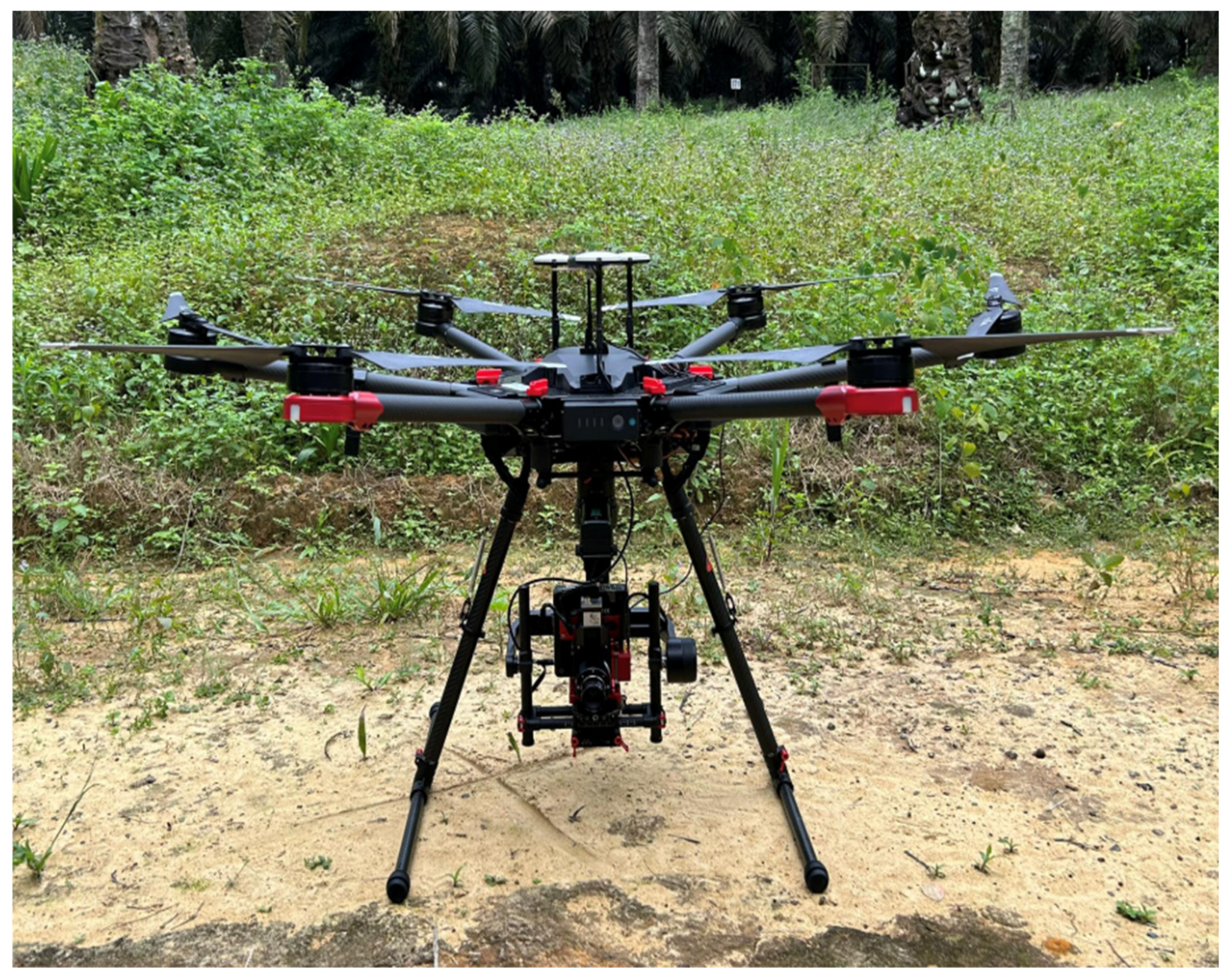
Three different sites in Malaysia were considered in this study. The locations of the areas are shown in Figure 1. Each of them has approximately 20 thousand Dura x Pisifera (DxP) oil palms whose ages are slightly more than ten years old. The three areas record a consistent annual rainfall of around 2700 mm. Most of the oil palms are healthy, and they bear fruit periodically all year long. A Resonon Pika L hyperspectral camera (Bozeman, MT, USA) was utilized to capture the data, and it was carried by a DJI M600 Pro hexacopter drone (Shenzhen, Guangdong, China). They are shown in Figure 2. The hyperspectral data has 300 spectral bands covering the wavelength of 381 nm to 1019 nm. The spectral resolution is approximately 2 nm and the sampling frequency of the data acquisition is 249 frames per second to ensure good data fidelity. The spatial resolution is 7 cm × 7 cm for one pixel.
The overlapping ratio of consecutive images is approximately 70% to 80%. Each area covered by the drone is large, around 200 hectares. Usually, it takes around two weeks to capture, align, stitch, correct and balance the hyperspectral images into a large output data of 300 channels. Due to the variations in environmental factors such as humidity, temperature and light intensity, some defects are noticeable in the output hyperspectral data. Stitching lines, luminosity drift, contrast variation and speckle noise can be clearly observed in some channels. Out of the three areas, 40 datacubes of size 5 00 × 500 × 300 were prepared for analysis where some of the datacubes overlap.

3.2. Approach

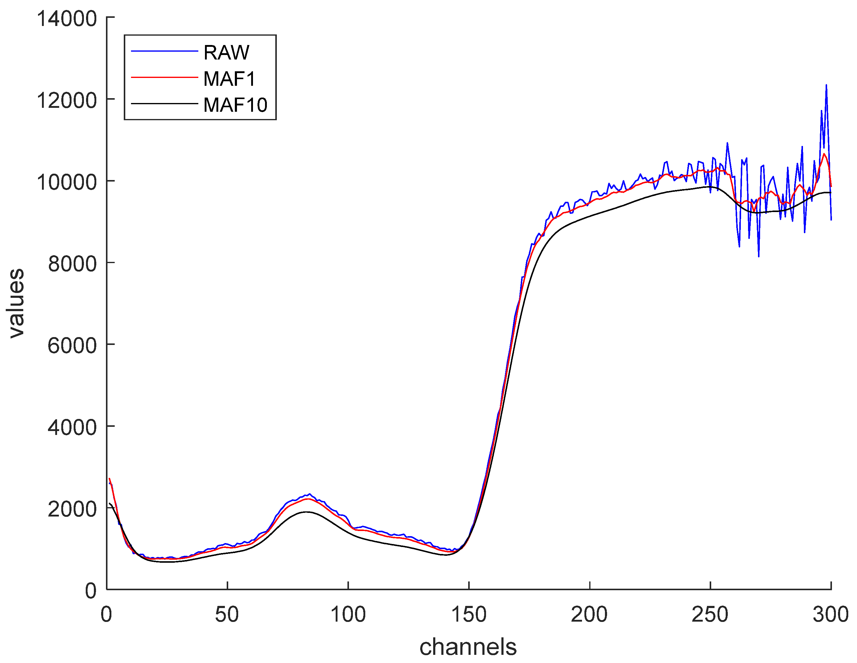
Many techniques have been proposed to filter noise in hyperspectral data but most of them require many iterations or replications. The aspect of preserving the integrity of the filtered data is often overlooked. When noisy channels are subjected to repeated filtering, they tend to lose some important spectral signatures, and the pixel value ranges of the channels shrink. When the pixel value ranges of neighboring channels start to shrink and bunch up, they become more similar [1]. This suppresses individual channel characteristics, which results in the loss of some spectral signatures. To demonstrate the point, spectral and spatial filtering were performed on a datacube with 300 channels using a simple moving average filter (MAF). Figure 3 shows the average pixel values of a 3 × 3 area after one and ten iterations of MAF. The figure shows that the intrinsic fluctuations in channels 200 to 250 (blue line) become smooth after the tenth iteration (black line). In some applications, it is important to preserve the fluctuations as they can be used as spectral signatures or features. For instance, Izzuddin et al. (2017) used the average pixel values of a circular area as features to classify oil palms that have been infected by Ganoderma. In their work, noisy channels are identified and excluded manually, prior to data analysis [1].
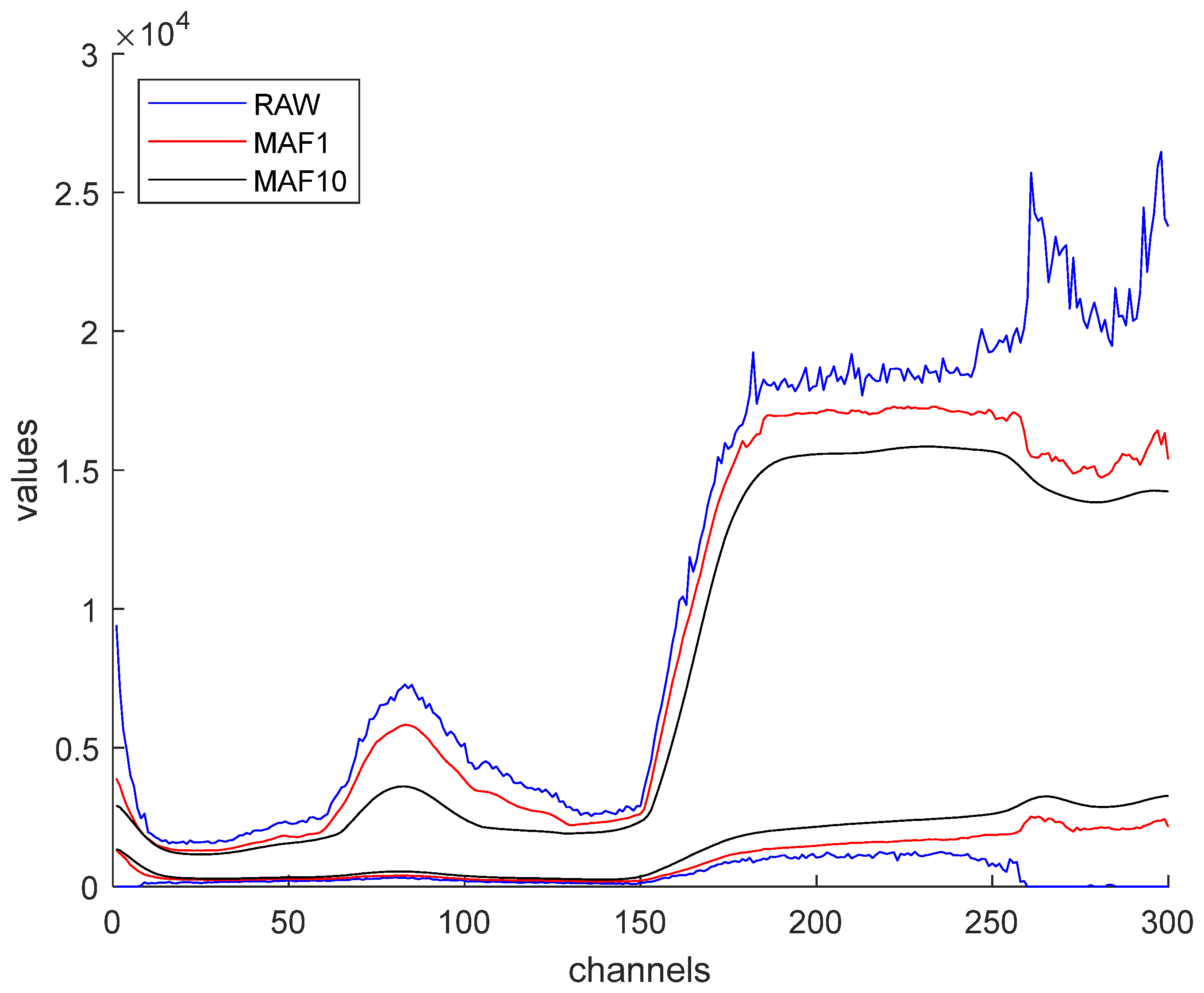
Shrinking pixel value ranges of the channels is another issue caused by over filtering. As the number of filtering iterations increases, pixel value ranges of neighboring channels start to converge. Figure 4 shows the upper and lower limits of pixel value ranges of the raw and filtered channels of a datacube after one and ten iterations of MAF. The limits are obtained from the whole area of each channel. It is seen that the gap between the upper and lower limits of the channels become smaller as the number of iterations increases. Thus, it is important to keep the number of iterations to a minimum when implementing lowpass filtering.
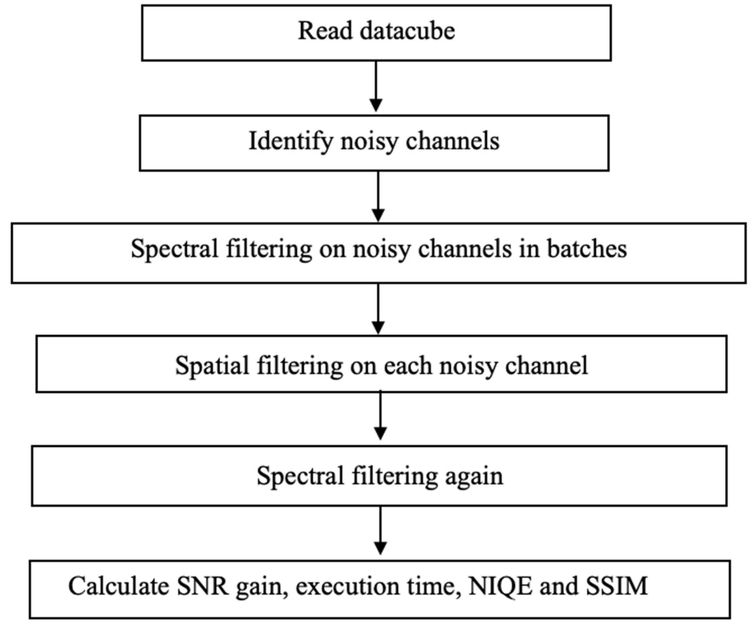
Figure 5 shows the main steps of the denoising framework. It starts by taking the hyperspectral data as input and storing it in a 3D array of 500 × 500 × 300 pixels. The size of the image of each channel is 500 × 500 pixels. From visual observation and SNR calculation, only images associated with low wavelength (381–400 nm) and high wavelength (931–1019 nm) are severely affected by noise. Also, the noise level becomes worse as the wavelength decreases toward 350 nm and as it increases toward 1000 nm. After identifying the noisy channels, the first round of spectral filtering is implemented using KF, EKF, KS and EKS. Both spectral and spatial filtering are performed using a one dimensional (1D) array of the noisy channels. For spectral filtering, the array is filled with pixel values of the noisy channels at one position ( x , y ) . Then, the array is filtered. This step is repeated position by position. For spatial filtering, the pixel values of one channel are collected row by row into a 1D array before it is filtered. Then, the pixel values of the filtered channel are recollected into a 1D array, column by column, and filtered again. The row and column filtering are performed channel by channel. Details of the formation of a 1D array for spectral and spatial filtering can be found in Ibrahim et al. (2024) [18]. In the framework, spectral filtering is implemented twice while spatial filtering is performed once only. In total, the number of iterations for spatial and spectral filtering are one and two, respectively. Then, performance and quality metrics are calculated.
When an image of a channel is corrupted by noise, the intensities of some or all pixels may deviate from their clean values. However, due to the stochastic and nonlinear nature of the noise, some pixels may still retain their clean values, or their values might just become slightly altered by the noise. The problem with most filtering techniques is they impose changes to all pixels without exception, even to clean pixels. In spatial filtering, if the intensity of a pixel differs significantly from those of its neighbors, it is assumed that its value is already affected by noise. However, clean pixels that fall at the border of two objects may have different pixel values. Therefore, an option is introduced in spatial filtering where the existing value of a pixel can be retained, subject to a local fitness function (LFF) of the pixel under consideration. The LFF is designed to be inversely proportional to the variation of the pixel’s neighborhood. Specifically, a change to a pixel value is permissible if the new value minimizes the local variation of its neighborhood. The simplest indicator of local variation is the standard deviation or the sum of absolute difference. This option is not made available in spectral filtering since the pixel values are collected from a single spatial position of all channels. Thus, they all belong to the same object. Furthermore, the pixel values in the array are accumulated from channels with different noise levels.
KF is implemented iteratively using 6 equations as shown below. Details of the models, equations and variables are available in many standard textbooks on Kalman filter [20].
x ^ t = F t x ^ t 1
P t = F t P t 1 F t + Q
y ^ t = H t x ^ t
K t = H t P t H t P t H t + R
x ^ t = x ^ t + K t ( y t y ^ t )
P t = P t P t H t K t
The equations are simplified by setting F t and H t to 1. For EKF, F t is set to 1 but H t is obtained from d h ( x t ) d t d t d x t . The rest of the equations for EKF are similar to the ones listed above. KS is implemented in two passes called the forward and backward passes. In the forward pass, the usual KF is implemented and in the backward pass, a few extra steps are added according to the Rauch, Tung and Striebel (RTS) (p. 270) algorithm as follows [20]:
K t =   P f t + P f t + 1
x ^ t = x ^ f t + + K t ( x ^ t + 1 x ^ f t + 1 )
P t = P f t + K t ( P f t + 1 P t + 1 ) K t
The backward pass descends from the last ( t = N ) to the first element ( t = 1 ) of the array. P f t + and P f t + 1 are obtained from implementing Equations (6) and (2) in the forward pass at elements t and t + 1 , respectively. And x ^ f t + 1 and x ^ f t + are obtained from implementing Equations (1) and (5) in the forward pass at elements t + 1 and t, respectively. x ^ t + 1 is the last value from Equation (8) at position t + 1 while the backward pass moves to the current position at t .
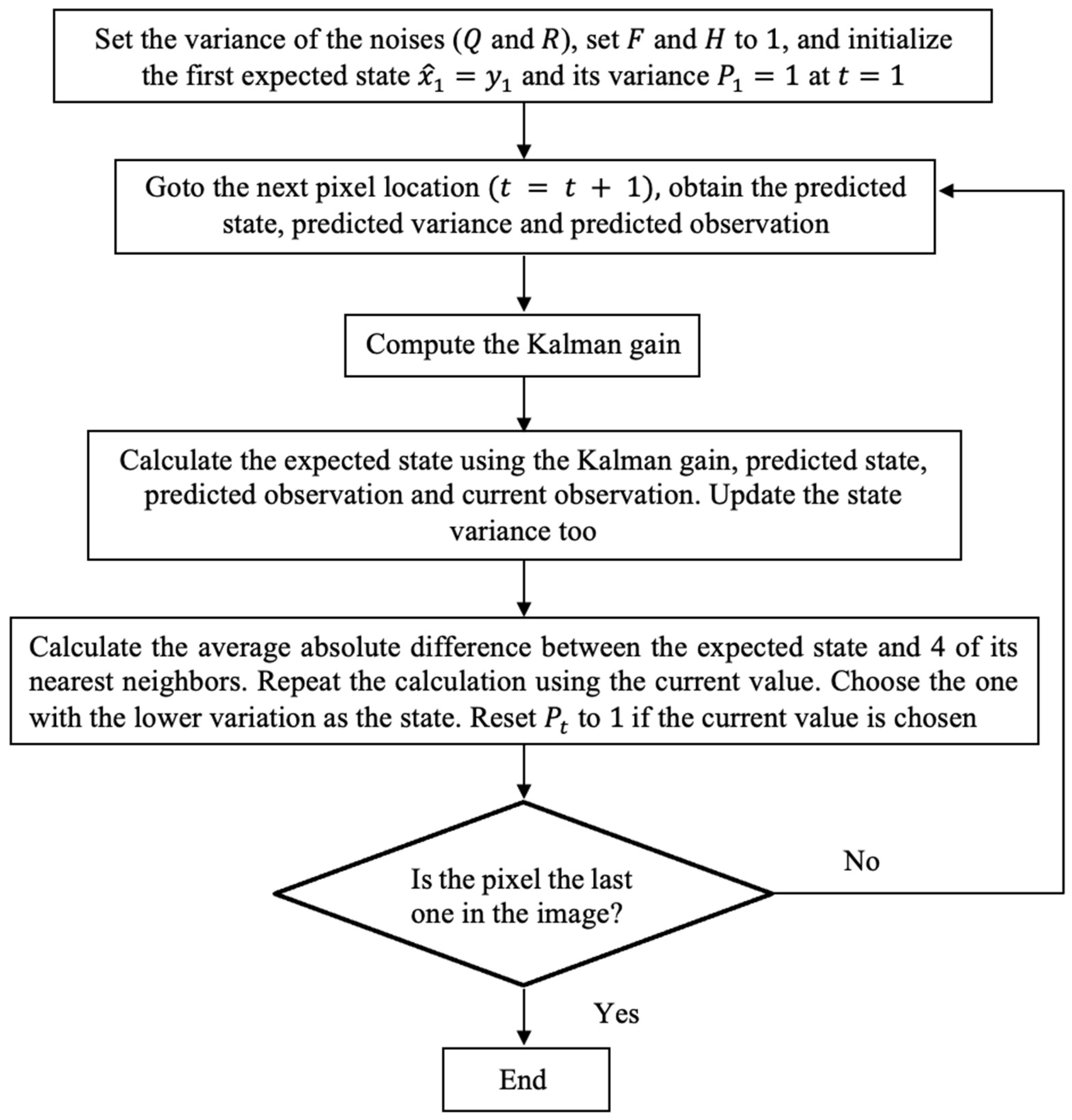
Since F t and H t are constantly set at 1, they are simply written as F and H. In batch processing, the values of all pixels are available and thus KF can be implemented in 4 directions. But normally, spatial filtering using Kalman family filters is implemented in horizontal and vertical directions only. In each direction, the expected state of each pixel can be calculated one by one. After computing the expected state of a pixel, the average absolute difference between the expected state and 4 of its nearest neighbors is calculated. The four nearest neighbors are the two pixels before and two pixels after the current pixel in the input array. Then, the same computation is repeated using the original value of the center pixel. Either the expected state or the original value of the pixel will be selected as the final value of the pixel, depending on which of the two minimizes the absolute difference, which can be regarded as the variation of the neighborhood. If the expected state is selected, KF continues to iterate as usual. However, if the original value is retained, the execution breaks, and the variance P t is reset to default before a new iteration commences at the next pixel. Consequently, KF that is implemented with this option is called Kalman filter with break (KFWB) as shown in Figure 6.
The pixel value ranges are bound to shrink when the channels are filtered. However, the shrinkage should be minimized to protect the spectral signatures of the data and the unique characteristics of individual channels. In post processing, the pixel value ranges of the filtered channels can be adjusted to coincide with those of the raw channels. This is achieved by shifting the values of all pixels in the filtered channel by the same constant so that the mean of the filtered channel is equal to its old value before filtering.
Suppose we wish to filter all channels and then adjust the means of the filtered channels to match those of the original raw channels. Let μ k and m k be the respective means of the raw and filtered channel k , where k = 1 , 2 , 3 , , 300 is the index of the channel. For a pixel in channel k at position ( x , y ) , its value is shifted by adding the difference between the raw and filtered means as follows:
r k ( x , y ) = f k ( x , y ) + ( µ k m k )
where r k ( x , y ) is the rectified pixel value and f k ( x , y ) is the filtered pixel value. This adjustment is carried out for all pixels in channel k , f k ( x , y ) , and this applies to all channels in the datacube.

4. Results and Discussion

Three counter measures were taken to mitigate the unwanted effects of bunching and shrinking pixel value ranges while denoising the channels. First, the number of iterations for spatial and spectral filtering were limited to one and two, respectively. Second, the option to retain clean pixel values based on a local fitness function was incorporated in spatial filtering. And third, the means of the channels were repositioned in post processing to restore some spectral undulations. The denoising scheme was used to denoise hyperspectral data containing 300 bands and the size of each datacube was 500 × 500 × 300 pixels.
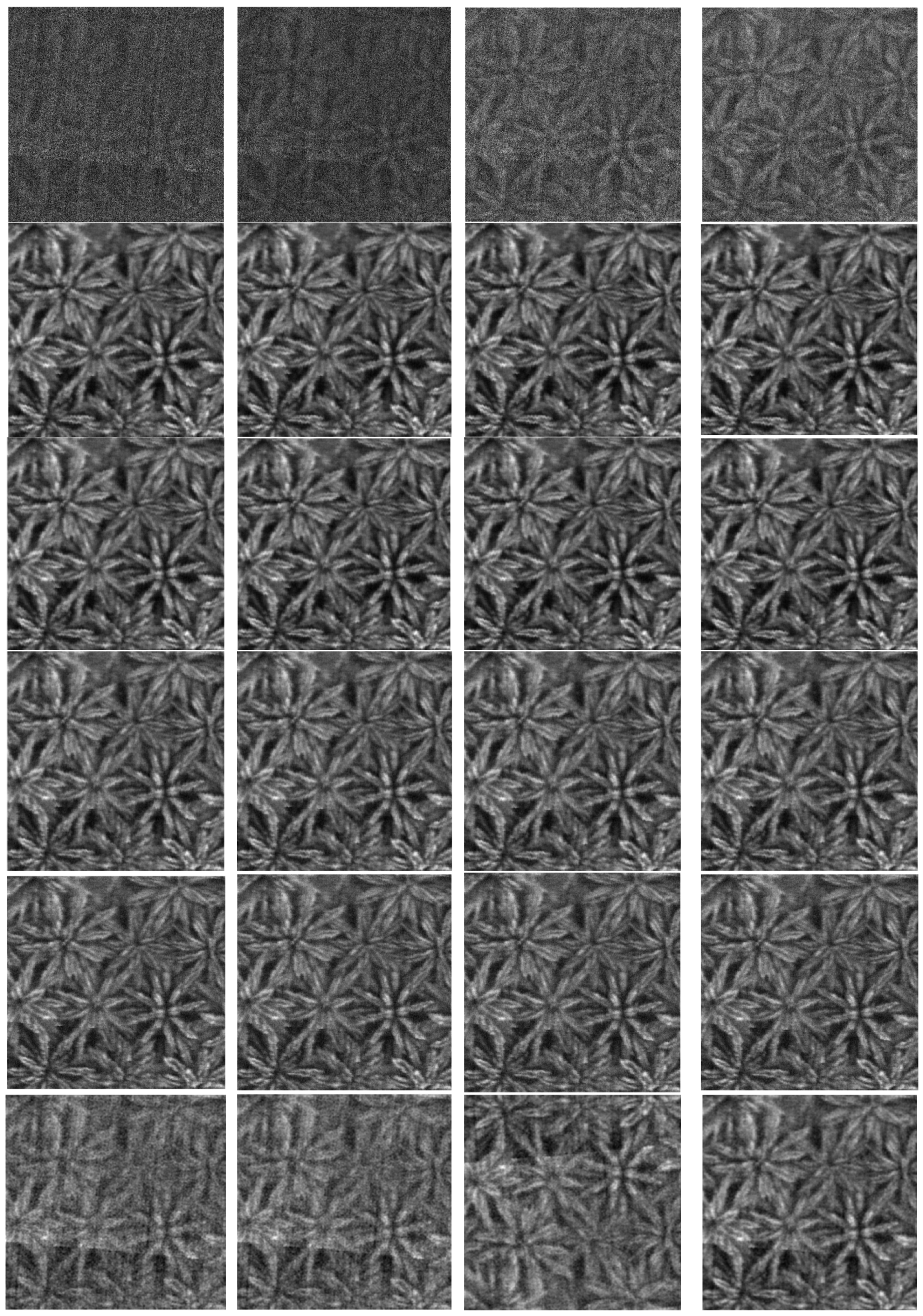
In the first set of experiments, noisy channels of 20 datacubes were filtered by KF, EKF, KS, EKS and MAF, under the same framework. Figure 7 and Figure 8 show the first and last four channels of a datacube before and after denoising. The results of MAF with window length five are included for benchmarking. Only the results of the first and last four channels are shown because they contain the most noise in their respective groups. The average SNR gain, execution time, NIQE and SSIM for the first and last four channels are listed in Table 1 and Table 2, respectively. The figures in the table suggest that the results of the KF, EKF, KS and EKS are very similar. Close visual inspection of the denoised channels verifies this observation.
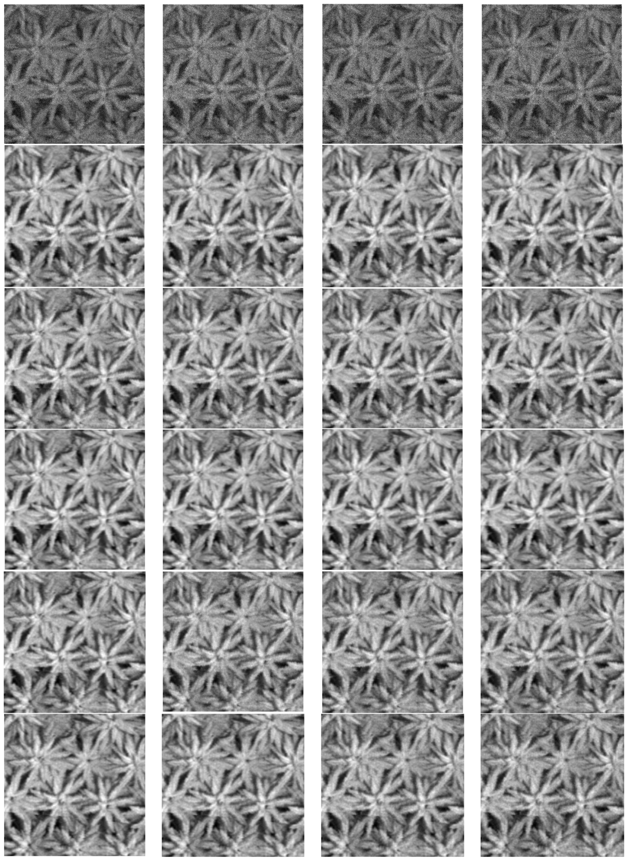
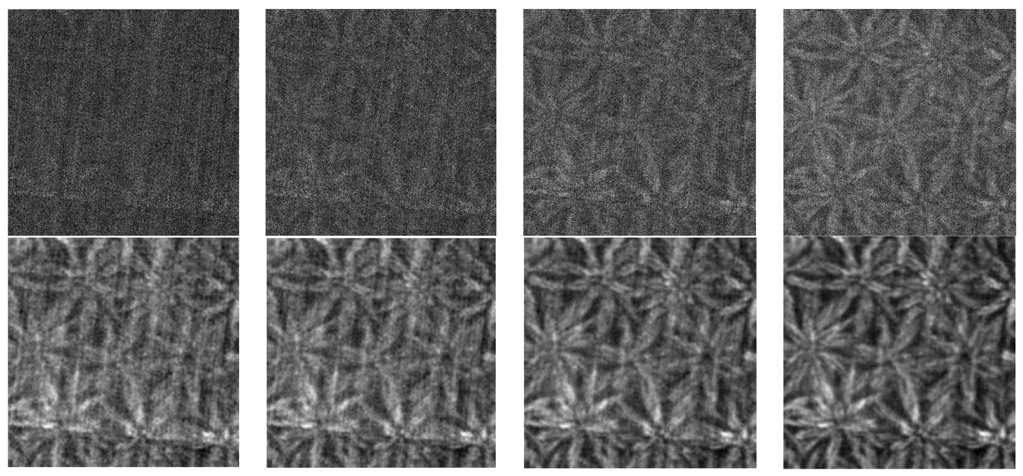
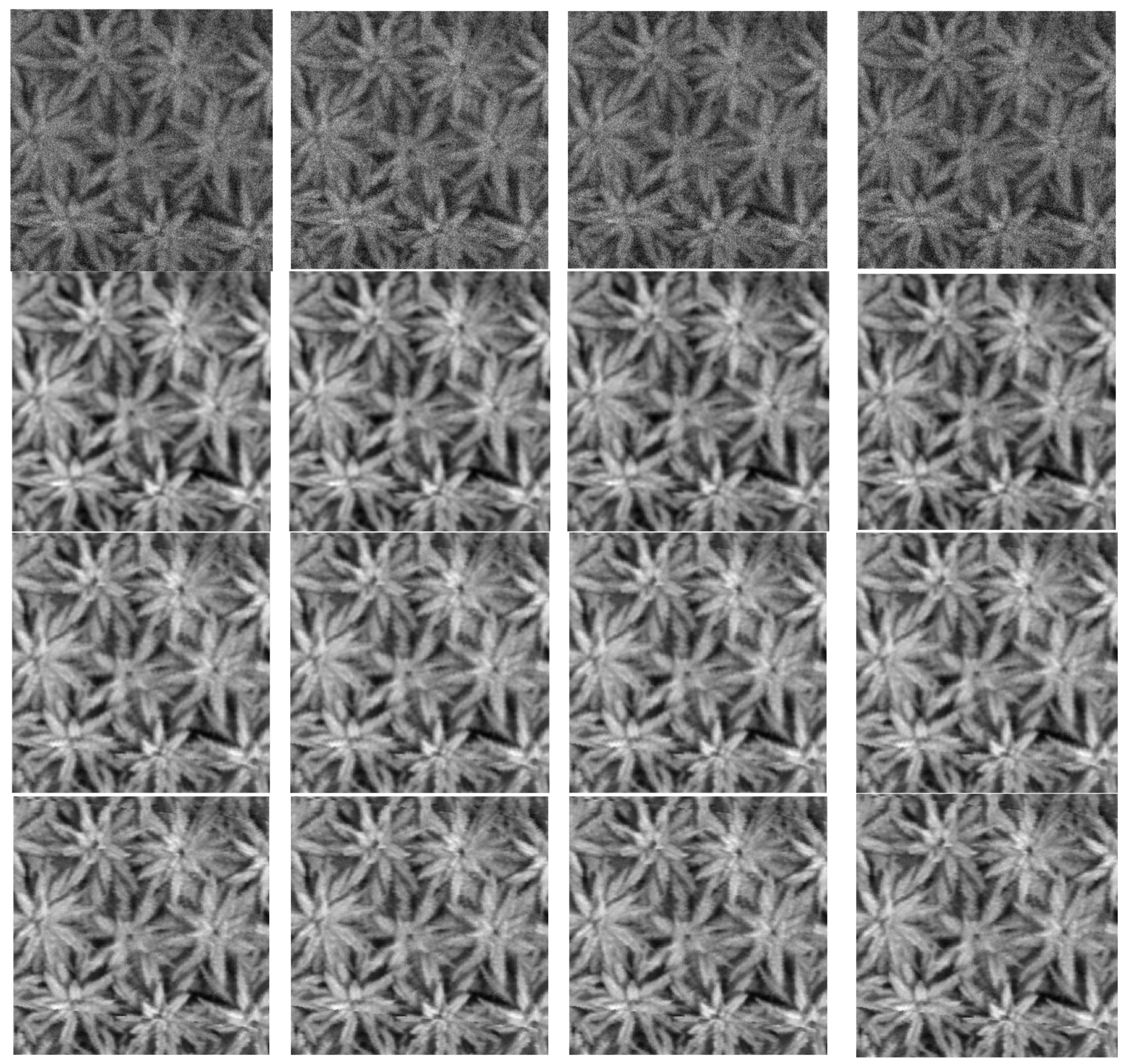
The results show that the performance of KF is comparable to those of EKF, KS and EKS because they were implemented under the same framework. Thus, it is sufficient to only test the KF with break option since it is the simplest and it represents the performance of the other Kalman family filters. Its performance would be compared against those of MAF and the normal KF. In the second set of experiments, the remaining 20 datacubes were filtered using MAF, KF and KFWB. Figure 9 shows the results of filtering the first four channels of a datacube using MAF, regular KF and KF with break (KFWB). In calculating the absolute difference between the center pixel and its neighbors, the length of the window used was five for all filters. This value was obtained from trial and error. It is observed that KFWB generates slightly sharper outputs than KF although the difference is only noticeable under close inspection.
Both KF and KFWB perform better than MAF in all cases. The grayscale shades of the KFWB outputs replicate those of the raw channels more closely. It is expected that the resemblance would translate to better spectral signatures and pixel value range preservation. The results of MAF are rough and noisy since MAF was less effective at spatial and spectral filtering. The number of spectral iterations for the filters was capped at two while the spatial filtering was implemented once.
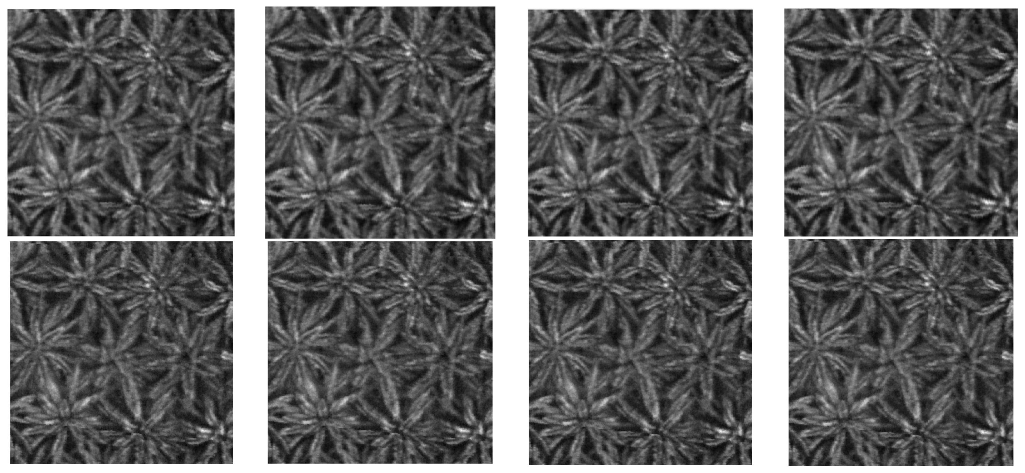
In the results filtered by MAF, a lot of pixels are bunched together at the high end of the pixel range. Hence the results appear brighter under normalization since a lot more pixels were scaled to higher values. Figure 10 depicts the last four channels of the datacube and the results of filtering them with the three filters. Here the results of all filters look nearly identical because the last four channels were less noisy than the first four. Still, the results of KFWB appear slightly sharper.
Table 3 presents the average SNR, execution time, NIQE and SSIM values produced by MAF, KF and KFWB for the first and last four channels. The values for KF are almost identical to the ones in the earlier tables. The SNR gained by KFWB are close to those of KF. The MAF registers lower metrics because it is less efficient at removing noise. The execution times recorded by the three methods are very similar.
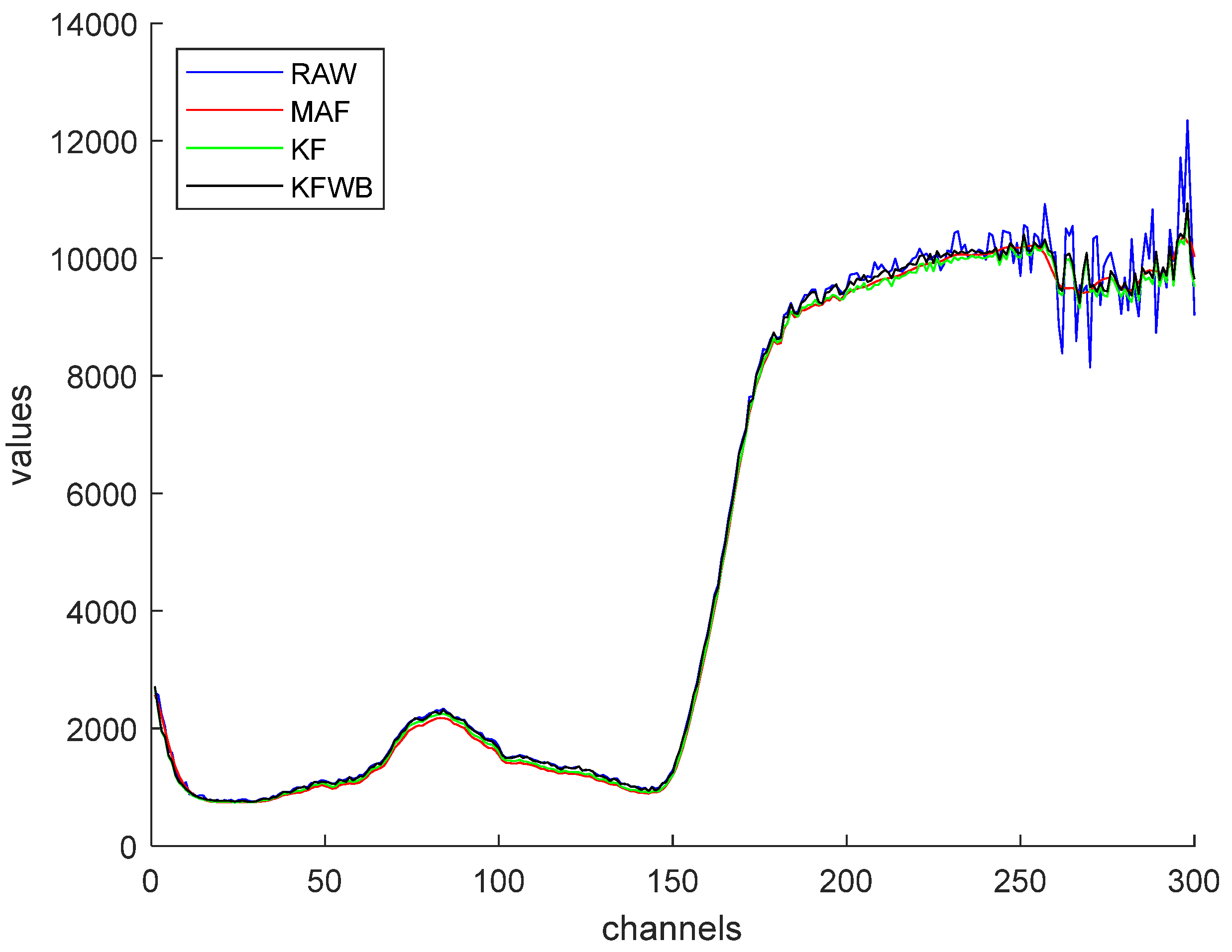
Figure 11 shows the average pixel values of the 3 × 3 area of the raw and filtered channels using MAF, KF and KFWB. The means of the KF and KFWB filtered channels have been restored to match those of the raw channels. The means of the MAF channels are unchanged because the MAF plot is used to gauge the effectiveness of the repositioning strategy.
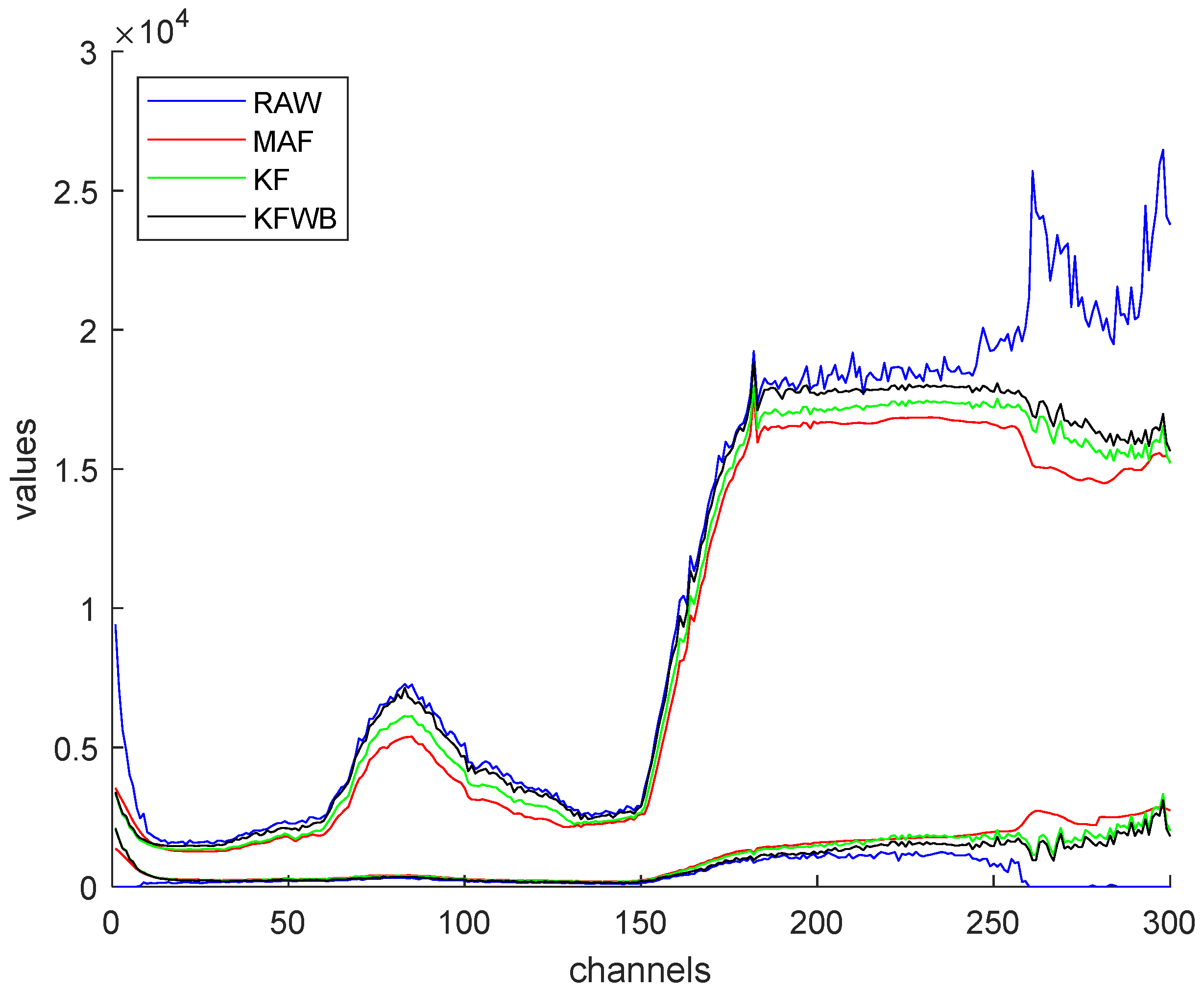
Under close inspection, it is observed that the KFWB plot follows the fluctuations in the average raw channels slightly better than the KF plot. In turn, both KF and KFWB are better at conserving the ripples than MAF because the means of the MAF channels are not adjusted while the means of the KF and KFWB channels have been restored to the raw values. Figure 12 shows the upper and lower limits of pixel value ranges of the raw and filtered channels by MAF, KF and KFWB. The upper and lower limits of the raw channels are erratic due to the influence of noise. As the noise is filtered, the ranges are bound to shrink and become closer for each channel.
Among the filters, it is seen that KFWB with mean restoration offers the widest pixel value ranges for most of the channels throughout the spectrum. The pixel value ranges normally shrink when the channels are filtered. However, the shrinkage should be controlled to protect the content of individual channels and their unique characteristics.

5. Conclusions

In this paper, KF, EKF, KS and EKS are utilized to filter noise in real hyperspectral data of oil palms. They are implemented with minimum iterations, to remove speckle noise while minimizing shrinkage of pixel value ranges and the loss of vital spectral signatures. Three measures were taken to mitigate the unwanted effects of bunching and shrinking pixel value ranges of channels. First, the number of iterations for spatial and spectral filtering were limited to one and two, respectively. Second, the option to retain clean pixel values based on a local fitness function was incorporated in spatial filtering. And third, the means of the channel were repositioned in post processing to restore some spectral signatures. Since the Kalman family filters are implemented under the same framework, their performances were very similar.
In the second set of experiments, only KF was tested with the option to retain clean pixel values. This is because KF is the simplest and its performance is identical to those of other Kalman family filters. The fitness function minimizes the local variation about the pixel under consideration. Between the original pixel value and the new value suggested by KF, the one that minimizes the local variation will be selected. Finally, the means of the filtered channels were repositioned to those of the raw channels to restore some spectral signatures. The proposed methods were executed on MATLAB R2023b platform powered by an Intel i7 processor. The average time taken to filter one channel is less than 1 s. The main advantages of the proposed methods are their fast execution, ability to avoid processing clean pixels, the preservation of spectral signatures and the reduction in pixel range shrinkage. It should be noted that the method cannot remove significant haze, mist and cloud from the channels. The method would be combined with retinex in future work to make it more effective against extreme illumination drift and contrast variation.

Author Contributions

Conceptualization, I.I. and H.A.; Methodology I.I. and H.A., Formal analysis, I.I.; Resources, H.A. and M.I.A.; Writing—original draft, I.I.; Writing—review and editing, H.A.; Supervision, H.A. and M.S.A.T.; Data acquisition, M.I.A., H.A. and I.I. All authors have read and agreed to the published version of the manuscript.

Funding

This research received no external funding.

Data Availability Statement

Data acquisitions were obtained from Malaysian Palm Oil Board (MPOB) and it is not publicly available due to non-disclosure agreement with the data provider.

Conflicts of Interest

The authors declare no conflicts of interest.

Abbreviations

The following abbreviations are used in this manuscript:
KFKalman Filter
EKFExtended Kalman Filter
KSKalman Smoother
EKSExtended Kalman Smoother
MAFMoving Average Filter
SNRSignal-to-Noise Ratio
NIQENaturalness Image Quality Evaluator
SSIMStructural Similarity Index Measure
UAVUnmanned Aerial Vehicle
PCAPrincipal Component Analysis
BM4DBlock Matching 4-Dimensions
LRMRLow-rank Matrix Recovery
HSIHue, Saturation and Intensity
CNNConvolution Neural Network
NNNeural Network
FTFourier Transform
LiDARLight Detection and Ranging
LFFLocal Fitness Function
KFWBKalman Filter with Break

References

  1. Izzuddin, M.A.; Seman Idris, A.; Nisfariza, M.N.; Nordiana, A.A.; Shafri, H.Z.M.; Ezzati, B. The development of spectral indices for early detection of Ganoderma disease in oil palm seedlings. Int. J. Remote Sens. 2017, 38, 6505–6527. [Google Scholar] [CrossRef]
  2. Chang, C.I. Hyperspectral Data Processing: Algorithm, Design and Analysis; John Wiley & Sons: Hoboken, NJ, USA, 2013; p. 196. [Google Scholar]
  3. Atkinson, I.; Kamalabadi, F.; Jones, D.L. Wavelet-based hyperspectral image estimation. In Proceedings of the IGARSS 2003. 2003 IEEE International Geoscience and Remote Sensing Symposium. Proceedings (IEEE Cat. No. 03CH37477), Toulouse, France, 21–25 July 2003; Volume 2, pp. 743–745. [Google Scholar] [CrossRef]
  4. Zelinski, A.; Goyal, V. Denoising hyperspectral imagery and recovering junk bands using wavelets and sparse approximation. In Proceedings of the 2006 IEEE International Symposium on Geoscience and Remote Sensing, Denver, CO, USA, 31 July–4 August 2006; pp. 387–390. [Google Scholar] [CrossRef]
  5. Chen, G.; Qian, S.E. Denoising of hyperspectral imagery using principal component analysis and wavelet shrinkage. IEEE Trans. Geosci. Remote Sens. 2010, 49, 973–980. [Google Scholar] [CrossRef]
  6. Chen, G.; Bui, T.D.; Quach, K.G.; Qian, S.E. Denoising hyperspectral imagery using principal component analysis and block-matching 4D filtering. Can. J. Remote Sens. 2014, 40, 60–66. [Google Scholar] [CrossRef]
  7. Zhang, H.; He, W.; Zhang, L.; Shen, H.; Yuan, Q. Hyperspectral image restoration using low-rank matrix recovery. IEEE Trans. Geosci. Remote Sens. 2013, 52, 4729–4743. [Google Scholar] [CrossRef]
  8. Chang, Y.; Yan, L.; Chen, B.; Zhong, S.; Tian, Y. Hyperspectral image restoration: Where does the low-rank property exist. IEEE Trans. Geosci. Remote Sens. 2020, 59, 6869–6884. [Google Scholar] [CrossRef]
  9. Xue, J.; Zhao, Y.; Liao, W.; Chan, J.C.W. Nonlocal low-rank regularized tensor decomposition for hyperspectral image denoising. IEEE Trans. Geosci. Remote Sens. 2019, 57, 5174–5189. [Google Scholar] [CrossRef]
  10. Maffei, A.; Haut, J.M.; Paoletti, M.E.; Plaza, J.; Bruzzone, L.; Plaza, A. A single model CNN for hyperspectral image denoising. IEEE Trans. Geosci. Remote Sens. 2019, 58, 2516–2529. [Google Scholar] [CrossRef]
  11. Chang, Y.; Yan, L.; Fang, H.; Zhong, S.; Liao, W. HSI-DeNet: Hyperspectral image restoration via convolutional neural network. IEEE Trans. Geosci. Remote Sens. 2018, 57, 667–682. [Google Scholar] [CrossRef]
  12. Pan, E.; Ma, Y.; Mei, X.; Fan, F.; Huang, J.; Ma, J. SQAD: Spatial-spectral quasi-attention recurrent network for hyperspectral image denoising. IEEE Trans. Geosci. Remote Sens. 2022, 60, 5524814. [Google Scholar] [CrossRef]
  13. Zhao, S.; Zhu, X.; Liu, D.; Xu, F.; Wang, Y.; Lin, L.; Yuan, Q. A hyperspectral image denoising method based on land cover spectral autocorrelation. Int. J. Appl. Earth Obs. Geoinf. 2023, 123, 103481. [Google Scholar] [CrossRef]
  14. Karami, A.; Heylen, R.; Scheunders, P. Denoising of hyperspectral images using shearlet transform and fully constrained least squares unmixing. In Proceedings of the 2016 8th Workshop on Hyperspectral Image and Signal Processing: Evolution in Remote Sensing (WHISPERS), Los Angeles, CA, USA, 21–24 August 2016; pp. 1–5. [Google Scholar] [CrossRef]
  15. Zhang, H.; Cai, J.; He, W.; Shen, H.; Zhang, L. Double low-rank matrix decomposition for hyperspectral image denoising and destriping. IEEE Trans. Geosci. Remote Sens. 2021, 60, 5502619. [Google Scholar] [CrossRef]
  16. Torun, O.; Yuksel, S.E.; Erdem, E.; Imamoglu, N.; Erdem, A. Hyperspectral image denoising via self-modulating convolutional neural networks. Signal Process. 2024, 214, 109248. [Google Scholar] [CrossRef]
  17. Ertürk, A. Sparse unmixing based denoising for hyperspectral images. In Proceedings of the 2016 IEEE International Geoscience and Remote Sensing Symposium (IGARSS), Beijing, China, 10–15 July 2016; pp. 7006–7009. [Google Scholar] [CrossRef]
  18. Ibrahim, I.; AlRowaily, M.H.; Arof, H.; Abu Talip, M.S. Performance Comparison of Selected Filters in Fast Denoising of Oil Palm Hyperspectral Data. Appl. Sci. 2024, 14, 2076–3417. [Google Scholar] [CrossRef]
  19. Bai, J.; Niu, Z.; Wang, L. A theoretical demonstration on the independence of distance and incidence angle effects for small-footprint hyperspectral LiDAR: Basic physical concepts. Remote Sens. Environ. 2024, 315, 114452. [Google Scholar] [CrossRef]
  20. Simon, D. Optimal State Estimation: Kalman, H Infinity, and Nonlinear Approaches; John Wiley & Sons: Hoboken, NJ, USA, 2006; p. 270. ISBN 9780470045343. [Google Scholar]
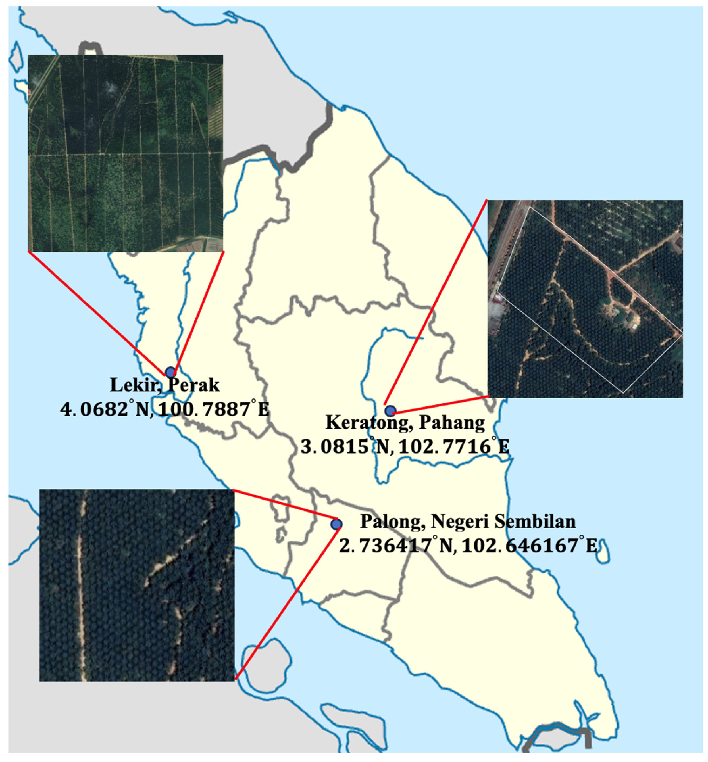
Figure 1. The locations of the areas of study in the states of Perak, Pahang and Negeri Sembilan, Malaysia.
Agriculture 15 02149 g001
Figure 2. Resonon Pika L hyperspectral camera attached to a DJI M600 Pro hexacopter drone.
Agriculture 15 02149 g002
Figure 3. The average pixel values of a 3 × 3 area of the raw and filtered channels of a datacube after one and ten iterations of spatial and spectral MAF.
Agriculture 15 02149 g003
Figure 4. The upper and lower limits of the pixel value ranges of the raw and filtered channels after one and ten iterations.
Agriculture 15 02149 g004
Figure 5. Flow of steps in the denoising framework.
Agriculture 15 02149 g005
Figure 6. Steps involved in the spatial filtering of KF with an option that allows retaining the current pixel value.
Agriculture 15 02149 g006
Figure 7. The first four channels of a datacube and the results of filtering them by KF, EKF, KS, EKS and MAF; row-wise from top to bottom.
Agriculture 15 02149 g007
Figure 8. The last four channels of a datacube and the results of filtering them by KF, EKF, KS, EKS and MAF; row-wise from top to bottom.
Agriculture 15 02149 g008
Figure 9. The first four channels of a datacube and the results of filtering them with MAF, KF and KFWB; row-wise from top to bottom.
Agriculture 15 02149 g009aAgriculture 15 02149 g009b
Figure 10. The last four channels of the datacube and the results of filtering them with MAF, KF and KFWB; row-wise from top to bottom.
Agriculture 15 02149 g010
Figure 11. The average pixel values of a 3 × 3 area of the raw and filtered channels using MAF and mean-restored KF and KFWB.
Agriculture 15 02149 g011
Figure 12. The upper and lower limits of the pixel value ranges of the raw and filtered channels by MAF and mean-restored KF and KFWB.
Agriculture 15 02149 g012
Table 1. The average SNR gain, execution time, NIQE and SSIM of the first four channels.
FilterKFEKFKSEKSMAF
SNR Gain18.1 dB18.1 dB18.1 dB18.1 dB16 dB
Execution Time0.19 s0.2 s0.2 s0.21 s0.19 s
NIQE10.510.510.510.58.5
SSIM0.420.420.420.410.24
Table 2. The average SNR gain, execution time, NIQE and SSIM of the last four channels.
FilterKFEKFKSEKSMAF
SNR Gain7.3 dB7.3 dB7.4 dB7.4 dB6.0 dB
Execution Time0.18 s0.19 s0.2 s0.21 s0.18 s
NIQE9.59.59.459.459.0
SSIM0.270.270.260.260.14
Table 3. The group averages of SNR gain, execution time, NIQE and SSIM of the first and last four channels after filtering using MAF, KF and KFWB.
ChannelsFirst Four GroupLast Four Group
FilterMAFKFKFWBMAFKFKFWB
SNR Gain16 dB18 dB18 dB6 dB7.4 dB7.5 dB
Ex. Time0.2 s0.19 s0.2 s0.2 s0.18 s0.2 s
NIQE8.510.510.59.19.59.6
SSIM0.240.420.420.140.270.27
Disclaimer/Publisher’s Note: The statements, opinions and data contained in all publications are solely those of the individual author(s) and contributor(s) and not of MDPI and/or the editor(s). MDPI and/or the editor(s) disclaim responsibility for any injury to people or property resulting from any ideas, methods, instructions or products referred to in the content.