Article

Season-Specific CNN and TVDI Approach for Soil Moisture and Irrigation Monitoring in the Hetao Irrigation District, China

1
College of Water Conservancy and Civil Engineering, Inner Mongolia Agricultural University, Hohhot 010018, China
2
Autonomous Region Collaborative Innovation Center for Integrated Management of Water Resources and Water Environment in the Inner Mongolia Reaches of the Yellow River, Hohhot 010018, China
3
State Key Laboratory of Water Engineering Ecology and Environment in Arid Area, Inner Mongolia Agricultural University, Hohhot 010018, China
4
College of Energy and Environment, Inner Mongolia University of Science and Technology, Baotou 014020, China
*
Authors to whom correspondence should be addressed.
Agriculture 2025, 15(18), 1946; https://doi.org/10.3390/agriculture15181946
Submission received: 13 August 2025 / Revised: 10 September 2025 / Accepted: 12 September 2025 / Published: 14 September 2025
(This article belongs to the Section Agricultural Water Management)

Abstract

We develop a year-round, field-scale framework to retrieve soil moisture and map irrigation in an arid irrigation district where crop phenology and canopy dynamics undermine static, single-season approaches. However, the currently popular TVDI application is limited during non-growing seasons. To address this gap, we introduce a season-stratified TVDI scheme—based on the LST–EVI feature space with phenology-specific dry/wet edges—coupled with a non-growing-season inversion that fuses Sentinel-1 SAR and Landsat features and compares multiple regressors (PLSR, RF, XGBoost, and CNN). The study leverages 2023–2024 multi-sensor image time series for the Yichang sub-district of the Hetao Irrigation District (China), together with in situ topsoil moisture, meteorological records, a local cropping calendar, and district statistics for validation. Methodologically, EVI is preferred over NDVI to mitigate saturation under dense canopies; season-specific edge fitting stabilizes TVDI, while cross-validated regressors yield robust soil-moisture retrievals outside the growing period, with the CNN achieving the highest accuracy (test R2 ≈ 0.56–0.61), outperforming PLSR/RF/XGBoost by approximately 12–38%. The integrated mapping reveals complementary seasonal irrigation patterns: spring irrigates about 40–45% of farmland (e.g., 43.39% on 20 May 2024), summer peaks around 70% (e.g., 71.42% on 16 August 2024), and autumn stabilizes near 20–25% (e.g., 24.55% on 23 November 2024), with marked spatial contrasts between intensively irrigated southwest blocks and drier northeastern zones. We conclude that season-stratified edges and multi-source inversions together enable reproducible, year-round irrigation detection at field scale. These results provide operational evidence to refine irrigation scheduling and water allocation, and support drought-risk management and precision water governance in arid irrigation districts.

1. Introduction

Soil moisture is a key variable for drought assessment and irrigation management in arid irrigation districts. This study focuses on Landsat-based TVDI during the growing season and SAR–optical fusion outside the growing season to close the gap in year-round irrigation monitoring in the Yichang sub-district of the Hetao Irrigation District, China.
Soil moisture is one of the factors that indicates the soil condition and provides information on crop water stress and yield estimation [1]. Satellite remote sensing for soil moisture inversion uses microwave and optical methods [2]. Microwave sensing employs radar with strong penetration, enabling all-weather monitoring by reducing reliance on weather conditions [3]. Optical sensing captures spectral data to build models correlated with soil moisture, such as vegetation indices, but is vulnerable to climatic factors like rain and clouds [4]. To enhance accuracy, researchers are integrating microwave and optical sensing. Weimann et al. [5] used ERS-1 SAR data and soil moisture measurements in linear regression, confirming the VV polarization–soil moisture correlation, and applied the model to estimate soil moisture in a German region. However, it lacked optical data or multi-variable algorithms (e.g., machine learning) for interference correction, relying on empirical models sensitive to vegetation cover and surface roughness and potentially causing soil moisture inversion errors.
Liu et al. [6] used Sentinel-1 time-series data with an LUT method based on MIMICS/AIEM-simulated backscatter coefficients to retrieve soil moisture in Darra, Senegal. Ground measurements and microwave products assessed temporal trends and spatial variations. Results showed good consistency with ground measurements in temporal trends and with SMAP/SMOS in spatial patterns. However, Sentinel-1 C-band data are susceptible to vegetation effects, and the study did not quantitatively assess vegetation attenuation or incorporate multi-band synergistic inversion. Santi et al. [7] used SFIM with SMAP and AMSR2 data to monitor soil moisture (SMC) in Italy during 2015. By combining sensor synergy and the HydroAlgo ANN algorithm, they achieved 10 km resolution SMC inversion. However, the low spatial resolution limits it to large-scale monitoring, excluding precise applications like agriculture or hydrology.
Infrared surface temperature is used to estimate evaporation and soil moisture distribution over large areas [8]. Optical remote sensing, using soil reflectance, emissivity and temperature, also provides estimates of soil moisture [9]. In agricultural fields, crop canopies often obscure direct soil observations [10], but vegetation indices and land surface temperature remain correlated with soil moisture, resulting in feedback among soil moisture, NDVI, and LST [11]. Because individual factors are limited, combining a vegetation index with temperature is essential for accurate drought monitoring [12]. NDVI is widely used for vegetation monitoring but tends to saturate at high leaf area index and is sensitive to atmospheric effects. The Enhanced Vegetation Index (EVI) was developed to address these limitations by using a blue-band correction and reducing canopy background signals. We hypothesize that an LST–EVI feature space could yield more stable dry-edge delineation under dense vegetation, which we test in this study. Sandholt et al. [13] proposed the Temperature Vegetation Drought Index (TVDI) by defining the dry and wet edges in the LST–VI feature space. TVDI requires no complex models and has shown significant results in drought monitoring across multiple regions. Tagesson et al. [14] combined TVDI with SMOS satellite data to improve spatial resolution. TVDI and the Crop Water Stress Index (CWSI) are both widely used drought indices but differ in regional applicability [15]. Bai et al. [16] compared TVDI (using both NDVI and EVI) and CWSI for drought monitoring on the Guanzhong Plain, finding that both were effective, with CWSI exhibiting a higher correlation with soil moisture. Previous studies have shown that TVDI is widely used for regional soil moisture monitoring, and that the LST–EVI–derived TVDI generally outperforms LST–NDVI–based TVDI in accuracy. However, few studies have combined continuous Landsat-8 and -9 imagery for high-resolution tracking of soil moisture and irrigation. Therefore, this study uses Landsat-8/9 to construct both LST–NDVI and LST–EVI feature spaces, characterizes their differences, and maps the spatiotemporal dynamics of soil moisture and irrigation distribution in the study area.
During the dense growing season, vegetation scattering and canopy water content attenuate C-band SAR signals, so we rely primarily on optical/TIR indices (e.g., TVDI) derived from Landsat imagery. In contrast, during the spring and autumn irrigation periods, when fields are largely bare or sparsely vegetated, Sentinel-1 backscatter more directly reflects soil moisture, justifying the use of SAR for those seasons. Relying on a single sensor or a single index may delay the detection of rapid changes; therefore, a multi-sensor strategy is adopted to improve monitoring timeliness and accuracy [17]. In recent years, data-driven approaches including deep learning have been increasingly applied to soil moisture estimation. In recent years, CNN-based approaches have been successfully applied to soil moisture mapping (e.g., learning complex relationships between satellite imagery and in situ moisture). Such deep-learning models can improve accuracy but require large labeled datasets and are less interpretable. By contrast, ensemble tree methods like RF and XGBoost are well-established in hydrological modeling, often achieving good performance with fewer training samples. To explore these trade-offs, we implement four models—PLSR, RF, XGBoost, and CNN—comparing their accuracy and practical utility for seasonal soil moisture inversion and irrigation mapping. This study focuses on the Yichang Irrigation District (Hetao) and aims to investigate soil moisture conditions during both the spring–autumn irrigation periods and the crop growing season. To achieve this, we first constructed a TVDI model using Landsat imagery to monitor the spatiotemporal distribution of soil moisture during the growing season. We then integrated multi-source data (optical, microwave, and in situ) and applied machine learning and deep learning methods to estimate soil moisture during the non-growing periods. This approach allowed us to analyze the dynamic evolution of soil moisture distribution during the spring irrigation, growing season, and autumn irrigation periods, and to identify changes in irrigation distribution in Yichang. This study provides technical support for agricultural water scheduling and crop production improvement in the region, and offers guidance for optimizing irrigation management and promoting water conservation in arid irrigation areas.

2. Materials and Methods

2.1. Technical Approach

We designed the overall methodology to leverage both a drought index and multi-source regression modeling, capturing soil moisture dynamics under vegetated and non-vegetated conditions. This study aims to utilize Landsat data to construct a Temperature Vegetation Drought Index (TVDI) model for monitoring and analyzing the spatiotemporal distribution of soil moisture during the crop growth period. By integrating multi-source remote sensing data, machine learning and deep learning methods are employed to inversely estimate the spatiotemporal distribution of soil moisture during the non-growing season. The spatiotemporal dynamic evolution of soil water in the Yichang Irrigation Basin over the spring irrigation–crop growth–autumn irrigation cycle is then analyzed, followed by an identification of changes in irrigation distribution patterns within the basin. Specifically, we construct the TVDI using Landsat-8/9 data, develop soil moisture models with selected features for prediction, and analyze soil moisture and irrigation distribution during vegetated and bare-soil periods based on the optimal model. The overall technical approach is illustrated in Figure 1.

2.2. Research Content

2.2.1. Spatiotemporal Dynamics of Soil Moisture During the Crop Growth Period (TVDI)

During the crop growth period, farmland soil is covered by vegetation, and the spatiotemporal changes in soil moisture can be indirectly inferred from vegetation status and surface temperature. Taking the Yichang Irrigation District in the Hetao Irrigation Area as the study area, multi-temporal Landsat-8/9 data from May to September 2023 and 2024 were selected to construct LST–NDVI and LST–EVI feature spaces, investigate patterns of dry–wet boundary changes, and calculate TVDI values. We selected the TVDI formulation with higher fitting accuracy to measured soil moisture to analyze the spatiotemporal distribution and dynamic evolution of soil moisture in the study area.

2.2.2. Soil Moisture Dynamics During Non-Growing Seasons Using Multi-Source Remote Sensing

During the non-growing season of crops, most surface soil in farmland is exposed and directly observable via remote sensing. For this period (spring flood and autumn irrigation), we used multi-source data (Landsat-8/9 optical and Sentinel-1 SAR) and selected features most strongly correlated with soil moisture as inputs to construct four soil moisture inversion models: partial least squares regression (PLSR), a linear multivariate method; random forest (RF), an ensemble decision-tree model; extreme gradient boosting (XGBoost), a tree-based boosting algorithm; and convolutional neural network (CNN), a deep learning model. These models were trained on the in situ measurements and evaluated, and the model with the highest accuracy was selected to map soil moisture distribution during the non-growing season. Finally, we analyzed the spatiotemporal dynamics of soil moisture distribution during the spring flood and autumn irrigation periods.

2.2.3. Identification of Farmland Irrigation Distribution Across Spring, Growing, and Autumn Periods

Understanding the continuous spatiotemporal changes in soil moisture is crucial for the rational allocation of irrigation water resources. Based on the TVDI and soil moisture models, a moisture threshold was applied to identify irrigated areas and extract the spatiotemporal changes in farmland irrigation distribution during the spring irrigation, growing, and autumn periods in the Yichang Irrigation Basin for 2023–2024. Irrigation area distribution maps were produced, and changes in irrigation area among these periods were investigated, with factors influencing the spatiotemporal differences discussed.

2.3. Overview of the Study Area

2.3.1. Overview of the Hetao Irrigation District

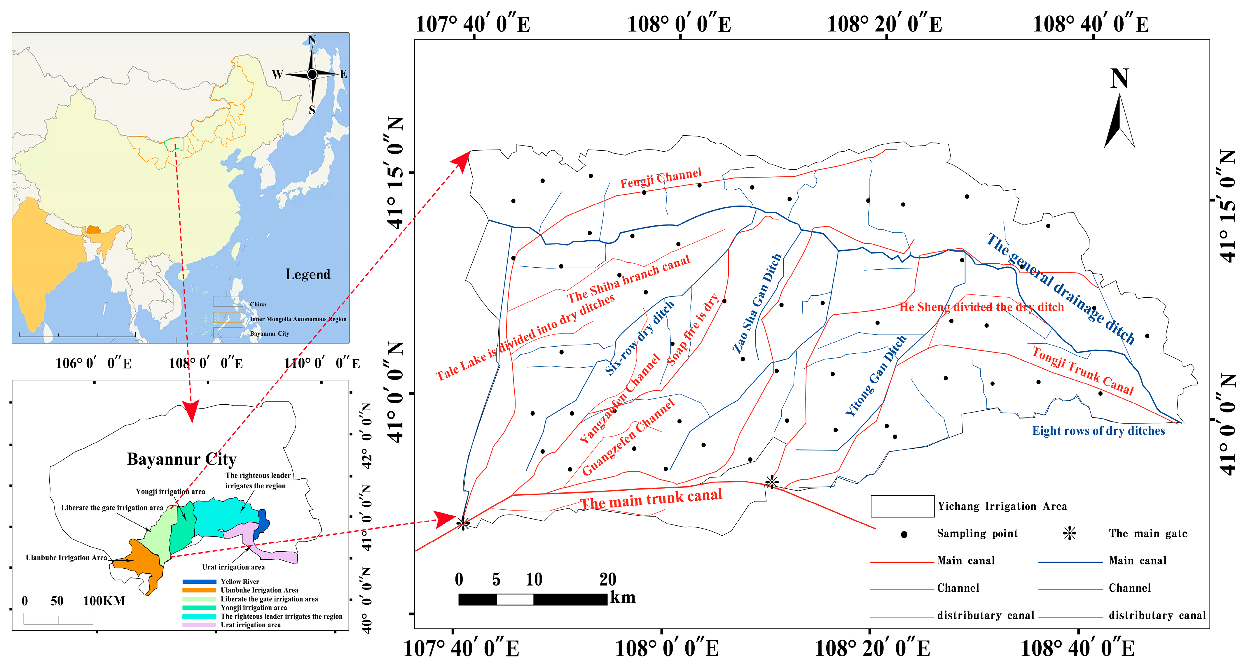
The Hetao Irrigation District is in Bayannur City, western Inner Mongolia, on the Hetao Plain. It spans 106°20′–109°19′ E and 40°19′–41°18′ N, covering approximately 250 km east–west and 50 km north–south across Dengkou County, Hangjin Houqi, Linhe District, Wuyuan County, and Wulate Qianqi [18]. The total land area is 1.19 million ha, with 0.77 million ha under Yellow River irrigation. It has 103,600 channels totaling 64,000 km and 183,500 structures, forming a seven-level irrigation and drainage system [19].The location of the study area is shown in Figure 2.

2.3.2. Overview of the Yichang Irrigation District

The Yichang Irrigation District is in northeastern Hetao Irrigation District, bordered by Yin Mountains to the north, Yellow River to the south, Yongji Irrigation District to the west, and Wulate Irrigation District to the east. Coordinates are 107°37′–108°51′ E and 40°45′–41°17′ N. It spans 106 km east–west and 48 km north–south, covering 32,144 ha, the largest within the Hetao Irrigation District [20]. As a backwater depression, the terrain is flat with an elevation of 1019.0–1035.3 m. The area has a temperate continental climate: low precipitation (177.5 mm year−1); high evaporation (2041.1 mm year−1); evaporation-to-precipitation ratio, 11.5; average temperature, 6.1 °C (highest in July and lowest in January); sunshine duration, 3230.9 h·year−1; solar radiation of 153.5 kcal·cm−2; prevailing northeast winds; average wind speed of 2.7 m·s−1 [21].

2.3.3. Irrigation and Drainage System Within the Yichang Irrigation District

The Yichang Irrigation District has five main canals and six branch canals, with a drainage system of five main ditches and 25 branch ditches. The annual average water diversion from the Yellow River is about 1.514 billion m3, with a drainage volume of around 369 million m3 [22]. The main canal and main drainage canal traverse the area, drawing water from the third and fourth gates: the third gate flows into the Fengji, Zaohuo, and Shahe canals, while the fourth gate supplies the Yihe and Tongji main canals. The irrigation and drainage system has six levels: main, secondary, tertiary, branch, farm, and field. A small area uses groundwater drip irrigation, covering approximately 183,700 ha. Major drainage channels include the Fifth, Sixth, Zao Sha, Seventh, and Yi Tong drainage channels, with drainage entering the main drainage channel and flowing into Wuliangsu Lake [23].

2.3.4. Phenological Periods

The phenological periods in the Yichang Irrigation Basin include three stages: spring runoff, crop growth period, and autumn irrigation [24]. During spring runoff and autumn irrigation, crops are scarce, soil is exposed, and irrigated farmland is submerged. The crop growth period spans the period from late May to late September, with major crops being wheat, corn, sunflowers, and zucchini. Sunflowers have the largest cultivated area, followed by corn, and wheat and zucchini have smaller areas. Wheat is sown earliest in late April and harvested by late July, while sunflowers are sown latest in late May and mature from late September to October [25]. Specific growth periods are shown in Table 1.

2.4. Remote Sensing Data and Preprocessing

2.4.1. Landsat Data and Preprocessing

Satellite monitoring accuracy varies by region or research objectives, with differing sensor data characteristics [26]. Landsat-8 (2013) and Landsat-9 (2021) data are shared openly via USGS Earth Explorer, achieving an 8-day revisit for continuous vegetation growth observation [27]. Because Landsat-8/9 provide a dedicated TIR band needed for LST-based TVDI, we prioritized Landsat imagery for the growing-season analysis, while Sentinel-1 SAR was used for the non-growing seasons. Both orbit at 705 km with 98.2° inclination, 185 km swath, and 16-day revisit, enhanced by an 8-day phase difference and pushbroom imaging [28]. Landsat-9 upgrades OLI-2 and TIRS-2, increasing radiation quantization to 14 bits for a better signal-to-noise ratio while retaining Landsat-8’s multispectral, panchromatic, and thermal infrared capabilities [29]. Data parameters are shown in Table 2.
Landsat-8 and Landsat-9 images with less than 20% cloud cover from May to September 2023 and 2024 were selected. Clouds and cloud shadows were masked using the QA band on Google Earth Engine (Google, Mountain View, CA, USA); masked gaps were filled by compositing the nearest available acquisitions (within 8 days) and performing linear interpolation over any remaining gaps. Scale factor corrections were applied, and the images were cropped to the study area. This resulted in 16 cloud-free Landsat scenes per year (8-day intervals, 30 m resolution).

2.4.2. Sentinel-1 SAR Data and Preprocessing

The Sentinel satellites are ESA’s Copernicus program observation satellites, including Sentinel-1, -2, and -6. Sentinel-1A and -1B launched in 2014 and 2016 with C-band SAR for all-weather observation. Their coordination reduces the revisit cycle to six days, using imaging modes SM, IW, EW, and WM. Parameters are given in Table 3 [30].
Sentinel-1 data products have three processing tiers: level-0 (raw), level-1 (preprocessed), and level-2 (end-user). Level-1 is split into SLC (single-view multipolar) and GRD (ground-range detection). SLC includes intensity and phase information, while GRD retains only intensity [31]. This study used SLC data from spring and autumn 2023–2024 in IW mode with VH + VV dual-polarization. Preprocessing employed ESA SNAP software 10.0.0 (SNAP Sensor SA, Narnenbourg, Naterth County, Switzerland), covering orbit calibration, radiometric calibration, image stitching, multi-view processing, noise filtering, terrain correction, and decibel conversion.

2.4.3. Backward Scattering Coefficient

The radar backscatter coefficient (σ0) normalizes the returned power to unit ground area and is commonly expressed in decibels (dB). It quantifies the target’s ability to reflect microwaves and is derived from the radar equation using the transmitted power, antenna gain, wavelength, range, and illuminated area, which is expressed by Equation (1):
P r   =   P t G 2 λ 2 ( 4 π ) 3 R 4 σ 0 A ,   σ   =   σ 0 A
where Pr is the radar received power, W; Pt is the radar transmitted power, W; G is the radar antenna’s transmission gain, λ is the radar operating wavelength, m; R is the distance between the target and the radar, and A is the area of the ground target object illuminated by the beam, which represents the scattering cross-section, m2.

2.4.4. Polarization Modes

Radar remote sensing systems observe targets using electromagnetic wave polarization. Core polarization modes are horizontal (H, electric vector parallel to ground) and vertical (V, electric vector orthogonal to ground) [32]. System operating modes based on transmit–receive configurations are as follows:
  • Single-polarization: Uses one channel (e.g., HH or VV) to measure backscatter intensity for dielectric property inversion, offering simplified data processing.
  • Dual-polarization: Combines H/V polarizations (e.g., HV-VH or VV-VH) to acquire multi-dimensional information like target direction, shape, and dielectric parameters.
  • Full polarization: Transmits and receives across all H, V, and cross-polarization dimensions (+45°/−45°), capturing complete scattering matrix data for significantly improved 3D target feature reconstruction accuracy compared to dual-polarization systems.

2.4.5. Polarization Target Decomposition

SAR polarization scattering characteristics better characterize surface target texture, morphology, and roughness than traditional radar backscatter coefficients, aiding in scattering mechanism analysis [33]. Main polarization decomposition algorithms include Freeman (three-component model) [34] and H/α (feature analysis-based) [35]. The latter uses coherent matrix decomposition for scattering analysis, with the mathematical expression according to Equation (2):
T = i = 1 3 λ i e i e i T
where  λ i is the eigenvalue of matrix T; e i is the eigenvector of matrix T; and e i T is the transpose of the eigenvector of matrix T. The entropy value H (range [0, 1]) extracted by this decomposition model reflects the degree of scattering randomness, with higher values indicating increased medium heterogeneity. The average scattering angle α (range [0, π/2]) quantifies the ratio between surface scattering and bulk scattering, with the specific calculation formula by Equations (3) and (4):
H   = i = 1 3 P i log 3 P i ,   P i   = λ i / i = 1 3 λ i
α = i = 1 3 P i α i
Originally, for fully polarized SAR, H/α decomposition extends to dual-polarization data processing due to increased data availability and method improvements. In agricultural remote sensing, H/α classification augmented with time-series data shows advantages. Recent studies [30,31] show that entropy and scattering angle positively correlate with soil moisture. This study’s Sentinel-1 feature extraction using SNAP is based on this framework.

2.5. Meteorological Data

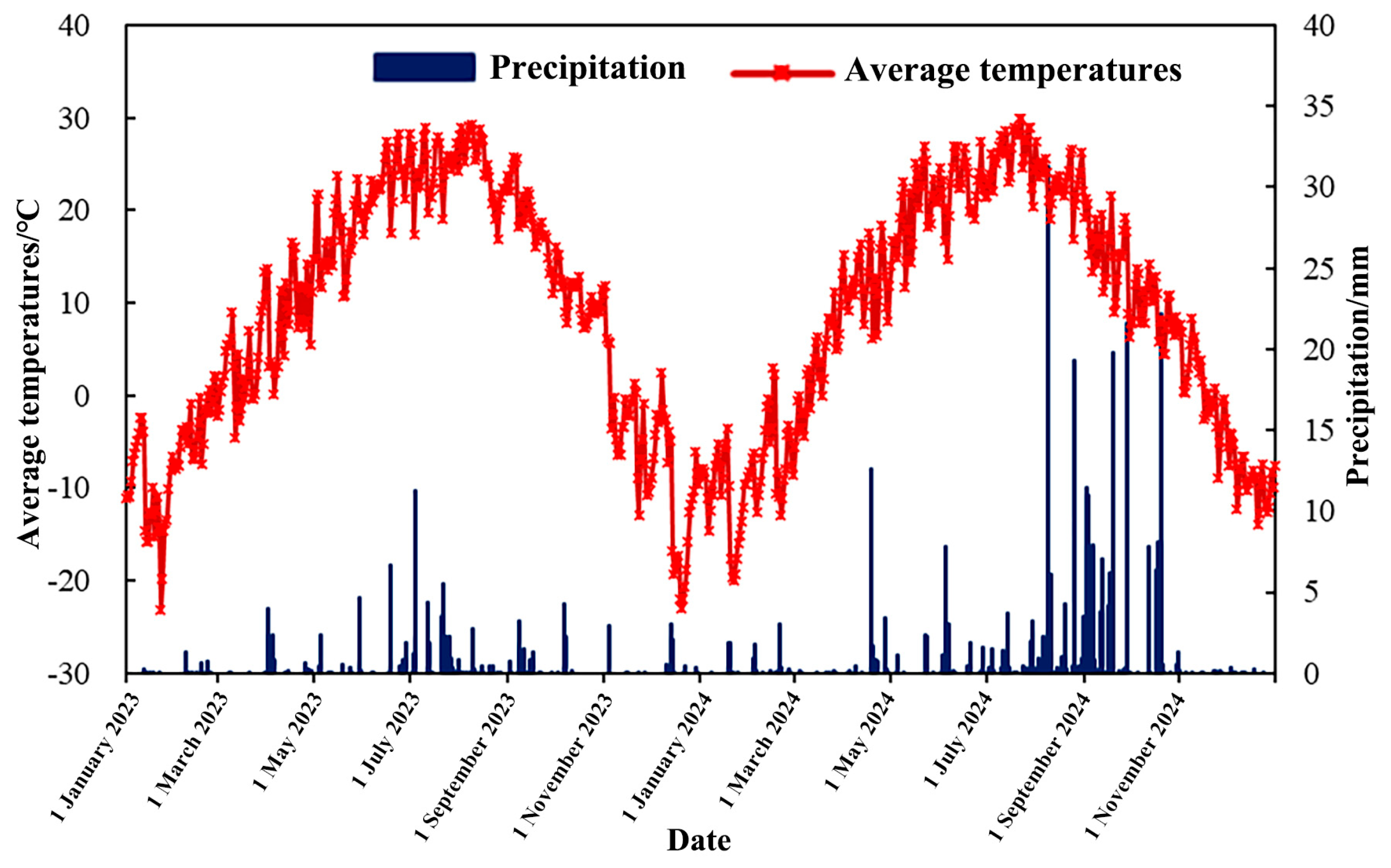
Meteorological data primarily originate from the China Meteorological Data Network (http://www.nmic.cn/, URL (accessed on 15 January 2025), including precipitation and temperature. Figure 3 shows the monthly total precipitation and mean air temperature for each month of 2023 and 2024.

2.6. Agricultural Land Area Data for the Yichang Irrigation District

This study used agricultural land data from Inner Mongolia’s third national land survey, based on <1 m resolution government satellite imagery. ENVI 5.6.2 (Environmental Systems Research Institute, Redlands, CA, USA) processed Yichang Irrigation Area imagery, identifying 369,120 ha of farmland (71.34% of its 517,390 ha total area).
Field measurements validated a farmland surface soil moisture inversion model. Sampling points were uniformly distributed and timed within three days of satellite overpasses. Four sessions occurred in 2023 (15 April: 60 points; 5 July: 40; 22 August: 30; 25 October: 30), and seven sessions occurred in 2024 (12–13 April: 100 points; 21–24 May: 68; 25–27 June: 45; 23–25 July: 54; 23–27 August: 40; 25–28 September: 60; 4–8 November: 40).
Within each 50 m × 50 m plot, soil samples were taken at five points at 0–10, 10–20, and 20–40 cm depths. Samples were stored in labeled aluminum boxes and weighed, with location, time, and vegetation coverage recorded. The average soil moisture content (SMC) per depth range was determined via drying at the base. The calculation formula was performed according to Equation (5):
S M C = W 1 W 2 W 1 W 2 × 100 %
where W1 is the mass of wet soil plus the aluminum box, g; W2 is the mass of dry soil plus the aluminum box, g; and W3 is the mass of the empty aluminum box, g.

2.7. Model Construction and Evaluation

2.7.1. Partial Least Squares Regression Model

PLSR integrates multiple linear regression, canonical correlation analysis, and principal component analysis into a multidimensional modeling framework [36]. It uses dimensionality reduction to extract core features, selects variables by maximizing covariance for prediction, and offers key advantages: (1) high tolerance for multicollinearity (|r| > 0.8); (2) overcomes sample size limitations for high-dimensional small-sample data; (3) retains original features via full variable projection, using VIP to quantify signal-noise separation; and (4) provides intuitive interpretation and lower computational complexity versus traditional regression while maintaining accuracy, which is ideal for explainable complex system modeling.

2.7.2. Random Forest Regression

Random forest (RF), proposed by Breiman et al. in 2001, is a machine learning method for classification, regression, and other tasks [37]. Its structure involves multiple decision trees (CART) based on binary rules, assuming aggregated predictions from numerous random trees enhance accuracy. A key RF advantage is accurately modeling complex relationships between variables under complex environments, enabling the learning of more complex nonlinear mappings than traditional methods for better simulation results.

2.7.3. Extreme Gradient Boosting

XGBoost is an advanced supervised boosting algorithm proposed by Tianqi Chen and Carlos Guestrin and improved in 2016 [38]. It is based on the GBDT framework, enhancing it by adding regularization and performing a second-order Taylor expansion of the loss function, incorporating constraints to improve accuracy and reduce overfitting. XGBoost optimizes distributed gradient boosting by continuously adding decision trees to fit residuals between predicted and actual values, then using ensemble learning for final predictions. Equation (6) was used:
y i   = k = 1 k f k xi
where fk is the kth learner; and yi is the predicted value of the ith sample.
To improve prediction accuracy, the XGBoost algorithm constructs a loss function L that represents the deviation of the model. Unlike gradient boosting, the XGBoost algorithm introduces a regularization term Ω to suppress model complexity, prevent overfitting, and enhance generalization capabilities. The final objective function was performed according to Equations (7) and (8):
Obj   =   L   + k = 1 k Ω ( f k )
L = i = 1 n l ( y i , y i )
where (fk) is the regularization term of the kth decision tree, and l(yi, yi) is the prediction error of the ith sample.
Assuming that XGBoost generates k decision trees after training, the prediction value can be obtained by summing the scores of each sample structure mapped to the leaf nodes of each decision tree, as shown in Equation (9):
F = f x = ω q x q : R f T , ω R T
where F is the predicted value; f(x) is the model of a decision tree; ω q x is the set of all leaf nodes of decision tree q; and T is the number of leaf nodes in the decision tree.

2.7.4. Convolutional Neural Networks

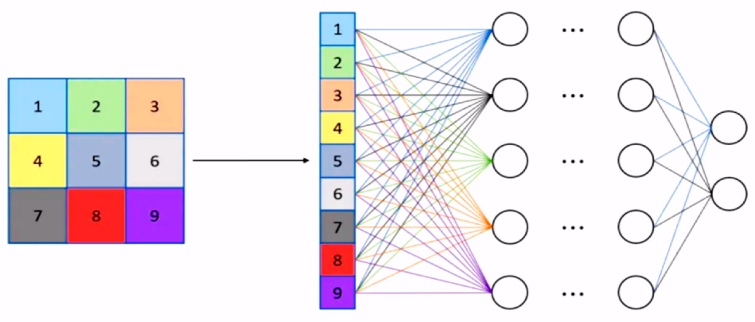
Convolutional neural networks (CNNs) are deep learning neural networks that excel in processing image data, relying on local connectivity and shared weights [39]. They comprise convolutional, pooling, and fully connected layers (Figure 4).
Pooling follows convolution, and convolution generates feature layers. After extraction, we need distinct features to avoid redundancy. Pooling segments and merging pixels, retaining key information, reducing dimension, lowering overfitting risk, and enabling key responses. After convolution and pooling, fully connected layers handle classification or regression, with each neuron connected to the neurons in the previous layer (Figure 5).

2.7.5. Model Evaluation Indicators

The accuracy of model fitting is evaluated using coefficient of determination (R2), which ranges from 0 to 1. The closer the value is to 1, the better the model construction and the stronger the fitting ability. Conversely, a value closer to 0 indicates poorer model construction and weaker fitting ability [39]. The formula for calculating R2 is shown in Equation (10):
R 2   =   1     i = 1 N w i     y i 2 i = 1 N w i y ¯ 2
The root mean square error (RMSE), also known as the standard error, is the mean of the squares of the errors between the model inversion values and the measured values. It reflects the degree of deviation between the inversion results and the measured results. The smaller the RMSE, the smaller the deviation and the higher the accuracy of the model. The calculation formula was performed according to Equation (11):
RMSE   = 1 N i = 1 N w i     y i 2
The mean absolute error (MAE) represents the average absolute error between the model inversion value and the measured value. Since it evaluates the absolute value of the error, the loss is fixed and less affected by discrete points. Similarly, the smaller the MAE, the better the accuracy of the model. Equation (12) was used:
MAE   = 1 N i = 1 N w i     y i
where N is the number of samples; wi is the soil moisture content value obtained from the model inversion; yi is the measured soil moisture content value; and y ¯ is the mean value of the measured values.

3. Results

3.1. Soil Moisture Inversion During the Crop Growing Season Based on TVDI

During the crop growing season, the ground in the Yichang Irrigation District is mostly covered by crops, making it difficult for satellites to directly observe the soil surface. Therefore, remote sensing techniques must be used to indirectly monitor soil moisture. Soil moisture balance in farmland determines crop growth. When moisture is sufficient, it meets crop growth requirements, and crops without moisture stress can perform normal physiological respiration and photosynthesis. Water vapor released through transpiration, along with shading from leaves, reduces canopy temperature, and canopy greenness reflects crop health. If crops experience water stress leading to physiological abnormalities, this is reflected in canopy temperature and vegetation greenness. At this point, satellite remote sensing can capture these changes to indirectly monitor soil moisture, with results validated using field measurement data. Indirectly obtaining soil moisture through canopy temperature [40] and vegetation growth status [8] is an effective method, and numerous scholars have extensively validated the feasibility of constructing TVDI using surface temperature and vegetation indices to analyze the spatiotemporal distribution characteristics of soil moisture drought indices during vegetation coverage periods [12,16,41,42].

3.1.1. TVDI Principle

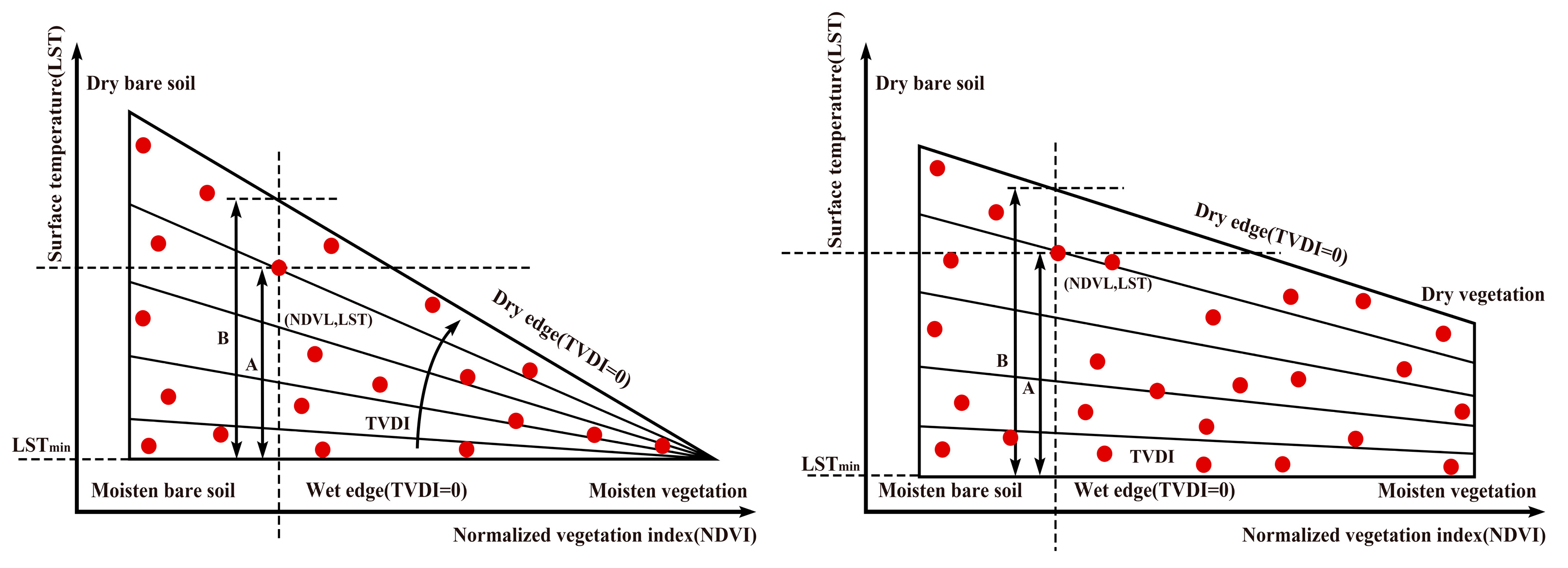
TVDI is based on vegetation indices (NDVI and EVI) and land surface temperature (LST). In two-dimensional space, the horizontal axis represents the vegetation index and the vertical axis represents LST. Pixel scatter points form the LST − VI feature space, which is simplified into a triangular or trapezoidal shape (Figure 6).
As shown in Figure 7, the horizontal axis NDVI in the feature space ranges from 0 to 1, representing the surface from bare soil to fully vegetated, while the vertical axis LST varies from low to high. TVDI is defined as A/B, where A = LST − LSTmin and B = LSTmax − LSTmin. Points with the same TVDI value form a downward-sloping straight line: TVDI = 1 represents the dry edge (most arid); and TVDI = 0 represents the wet edge (most humid), with the wet edge modeled as a horizontal line.
When vegetation coverage is low, the LST-NDVI feature space forms a triangle; when coverage is high, it forms a trapezoid. The endpoints include dry bare soil, moist bare soil, and moist vegetation; the trapezoid includes an additional dry vegetation (full vegetation coverage but no moisture). As surface cover transitions from bare soil to vegetation and soil moisture transitions from wet to dry, the feature space approximates a triangular or trapezoidal shape. The TVDI expression is as follows:
TVDI   =   LST     LST min LST max LST min
LST min   =   a 1   +   b 1 NDVI
LST max   =   a 2   +   b 2 NDVI
In the equation, LST is the surface temperature observed at a given pixel; LSTmin is the fitted wet-side value; LSTmax is the fitted dry-side value; a1 and b1 are the parameters of the wet-side linear fitting equation; and a2 and b2 are the parameters of the dry-side linear fitting equation.
The formulas for calculating NDVI and LST are as follows:
NDVI   =   ρ NIR ρ R / ρ NIR   +   ρ R
LST = ST B 10   ×   0 . 00341802 + 149
In the formula, ρNIR is the reflectance in the near-infrared band; ρR is the reflectance in the red light band; and STB10 is the surface temperature band.

3.1.2. Construction of LST-NDVI Feature Space and Dry-Wet Boundary Fitting

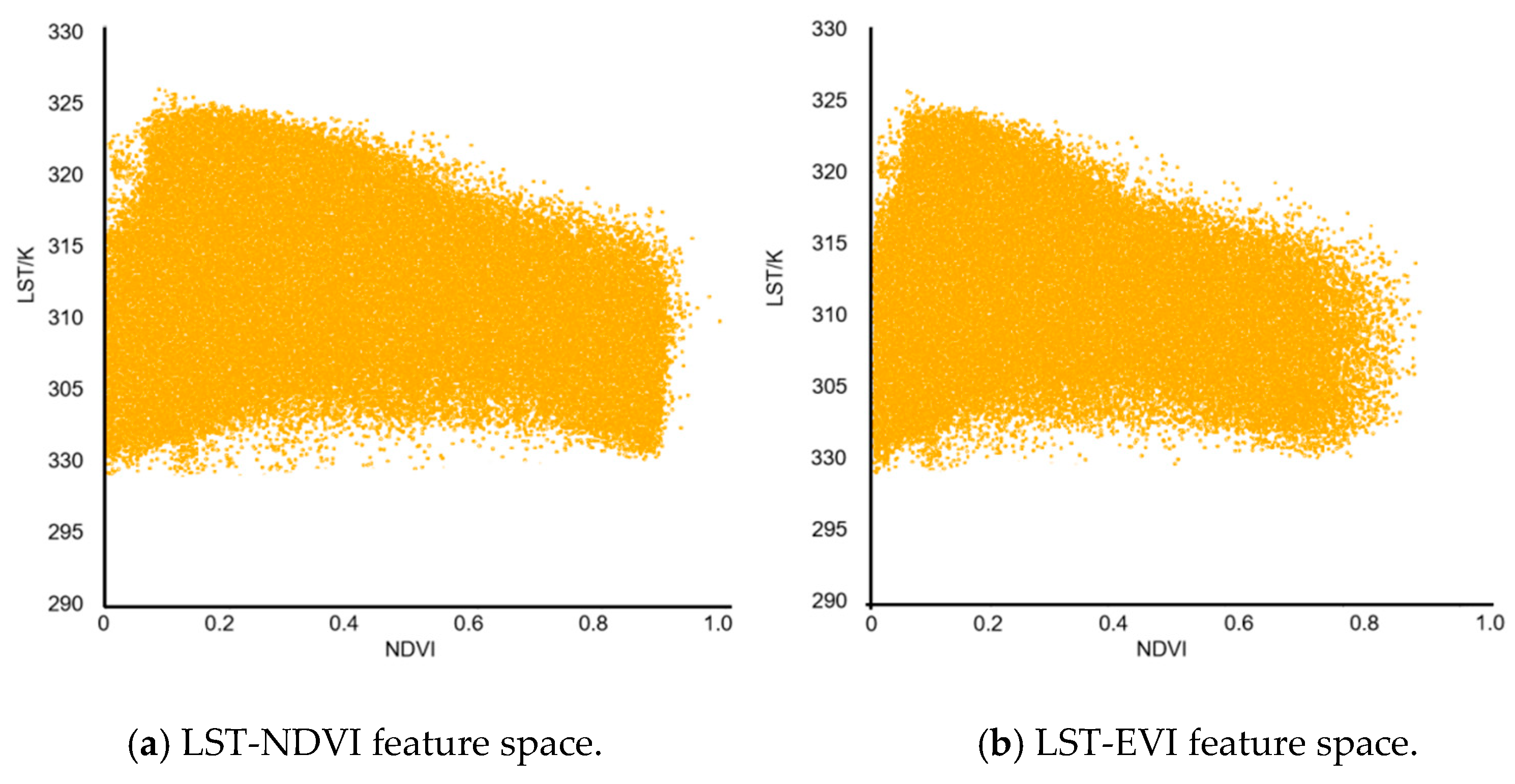
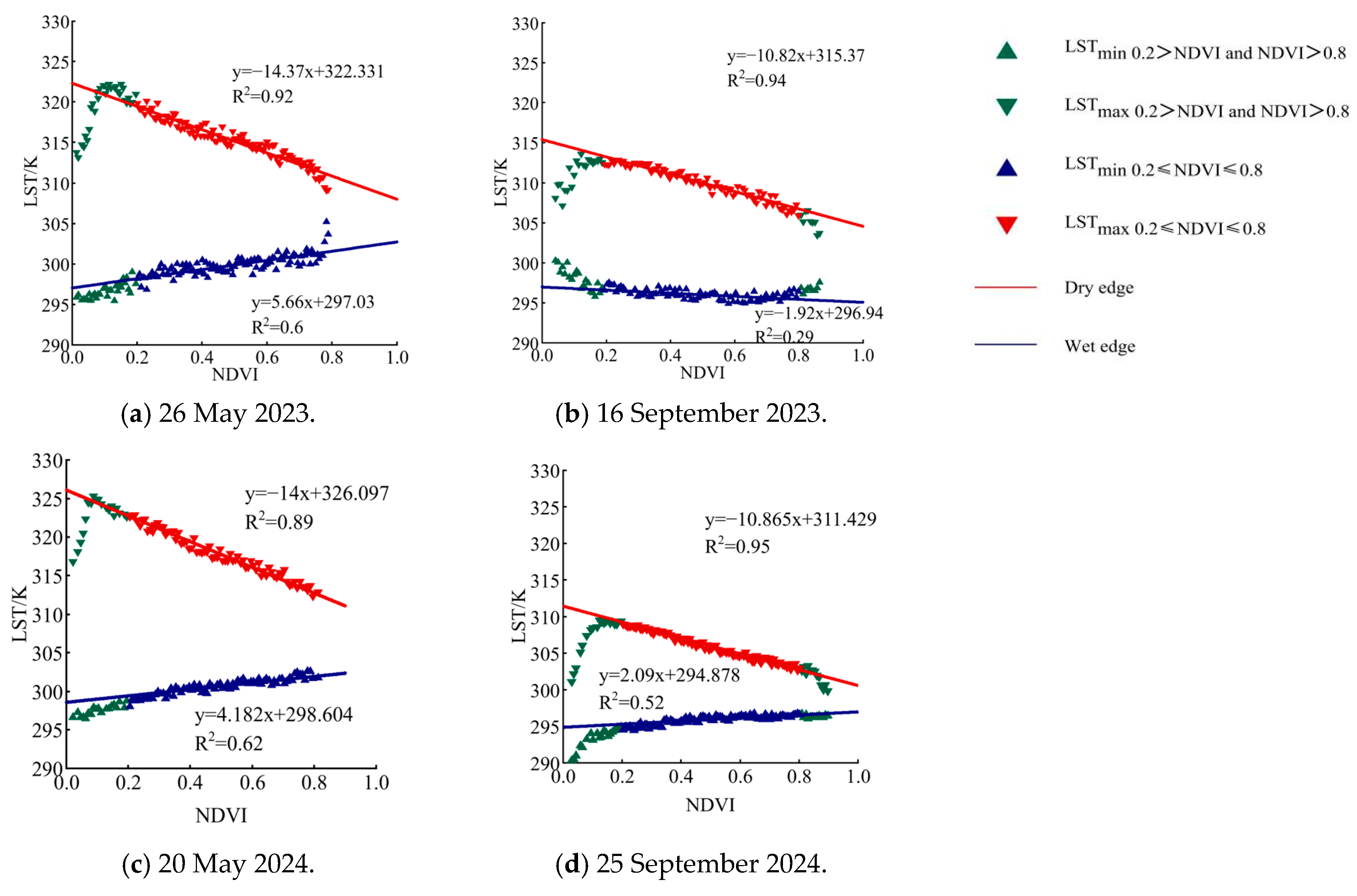
When fitting the dry and wet edges in the LST–NDVI space, pixels with NDVI ≤ 0.2 and NDVI ≥ 0.8 were excluded to avoid bare-soil and saturation effects. These bounds were selected to minimize bare-soil and saturation effects and are supported by ROC analysis against in situ (0–10 cm) soil-moisture and field-irrigation labels, with cutoffs maximizing Youden’s J clustering near 0.2 and 0.8. The choice also aligns with prior evidence that NDVI < ~0.2 indicates sparse/bare soil and NDVI > ~0.8 corresponds to fully developed canopies [13,43,44]. The dry edge was then obtained by linearly fitting the maximum LST at each NDVI level, and the wet edge by fitting the minimum LST. This stratified procedure reduced bias from extreme vegetation conditions and produced robust edge lines for TVDI calculation.The maximum temperature and wet/dry edge fitting in the feature space of LST-NDVI for 2023-2024 are shown in Figure 8.
By analyzing the temperature extremes and the fitting of the dry–wet boundary in the LST-NDVI feature space, it can be concluded that, when NDVI ≤ 0.2 and NDVI ≥ 0.8, the scatter points of the temperature extremes deviate from the main axis of the dry–wet boundary. This indicates that under conditions of extremely low or extremely high vegetation coverage, the distribution trend of temperature extremes corresponding to NDVI becomes abnormal, which will affect the fitting accuracy of the dry–wet boundary. When NDVI ≤ 0.2, the ground surface is primarily bare soil, making NDVI an unreliable indicator of vegetation conditions; when NDVI ≥ 0.8, NDVI becomes saturated, reducing its sensitivity to changes in vegetation coverage. In our TVDI computation, we first exclude pixels with NDVI ≤ 0.2 or NDVI ≥ 0.8 because these correspond to bare soil/water bodies or vegetation saturation, respectively. Within the remaining range (0.2 < NDVI < 0.8), we identify the dry edge by linearly fitting the maximum LST values at each NDVI level, and the wet edge by fitting the minimum LST values. This stratified fitting approach is supported by prior studies: excluding low and high NDVI removes extreme cases (bare soil or dense canopy) that can bias the fit. In practice, this procedure improved the dry-edge R2 from ~0.85–0.98 (using all points) to ~0.93–0.99 (after filtering). In summary, filtering out NDVI extremes and fitting LST maxima/minima yields more robust dry and wet edge lines for TVDI calculation.
For the dry and wet edges obtained in 2023 and 2024, the temperature of the dry edge decreases as the NDVI value increases, while the temperature of the wet edge increases as the NDVI value increases from May to June and decreases as the NDVI value increases from July to early September. The scatter points on the dry side are more regular, primarily distributed along the dry side, while the scatter points on the wet side are more dispersed compared to those on the dry side. The R2 values for the dry side equations derived from the feature space are all greater than 0.85, while the R2 values for the wet side equations range from 0.2 to 0.96.
To assess whether the dry and wet edges depend on phenology and canopy density, the LST–NDVI feature space was stratified by phenological windows (May–June, July–August, September) and, within each window, by EVI-based canopy-density groups. Refitting within each stratum revealed systematic shifts in slope and intercept—particularly a larger dispersion for the wet edge under dense canopies—indicating that a single global edge mixes distinct regimes. Accordingly, subsequent TVDI computations adopt season-specific edges rather than a global one.

3.1.3. Construction of LST-EVI Feature Space and Dry–Wet Boundary Fitting

Since its introduction, NDVI has been widely used in vegetation monitoring. NDVI has become the optimal remote sensing index for monitoring vegetation coverage and growth conditions. However, the NDVI based on NIR and RED normalized values reduces atmospheric effects at the cost of saturation, primarily manifested in limited handling of atmospheric interference. In areas with low vegetation coverage, it is prone to being influenced by soil background and vegetation canopy, resulting in elevated values, while in areas with high vegetation coverage, it is prone to saturation.
Vegetation index saturation refers to the phenomenon where in densely vegetated areas, as vegetation becomes increasingly dense, the vegetation index no longer increases with the increase in biomass. The Enhanced Vegetation Index (EVI) uses the “atmosphere-resistant vegetation index” and “soil-adjusted vegetation index” to mitigate the effects of aerosols and soil background, overcoming vegetation saturation. It can sensitively monitor the growth and decline of sparse and dense vegetation, addressing the limitations of NDVI. Selecting EVI to construct the LST-EVI feature space aims to optimize the correction of the dry–wet boundary scatter distribution trend shift in the LST-NDVI feature space in dense vegetation areas, thereby improving the dry–wet boundary fitting accuracy and enhancing the soil moisture inversion accuracy of TVDI during the crop growth period.
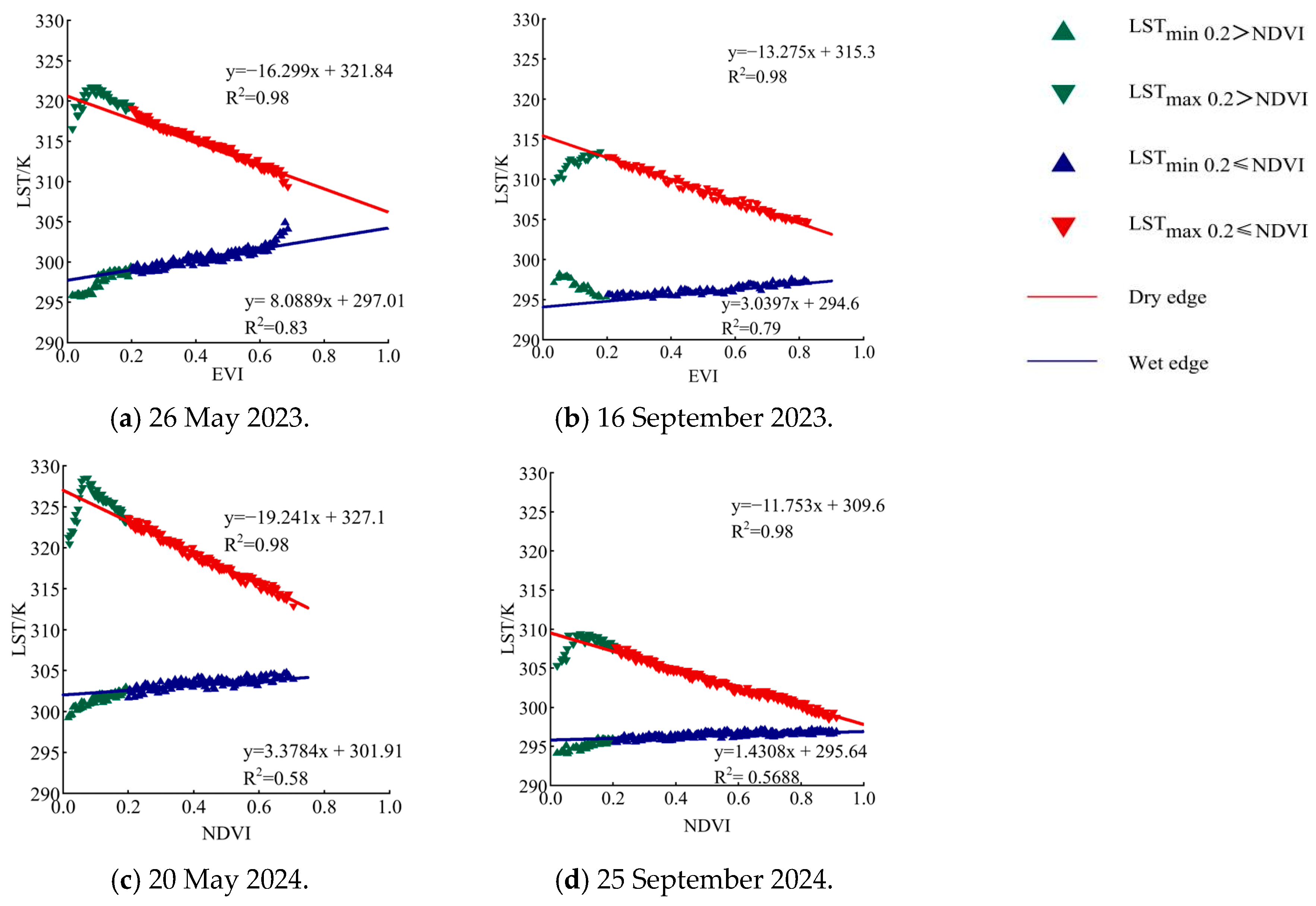
Based on EVI and LST, a feature space was constructed. As shown in Figure 9, in areas with low vegetation coverage, the dry and wet edges exhibit varying degrees of scatter anomalies, with particularly noticeable changes on the dry edge. Theoretically, as EVI approaches 0, soil moisture content increases, and the lowest value corresponds to water bodies, which may lead to significant differences between temperature trends and surface temperature changes. It can be observed that in areas with low vegetation coverage, both dry and wet edges exhibit shifts in the feature space formed by NDVI and EVI. In the LST-EVI feature space with EVI ≥ 0.8 or in areas with dense vegetation, the deviation of the dry side is significantly improved. The maximum temperature scatter plot distribution does not appear or shows only slight deviations, having a minimal impact on the linear fitting results. Therefore, the fitting accuracy of the dry side is higher, with R2 values ranging from 0.93 to 0.99. The situation on the wet side is more complex, with more diverse variations in minimum temperature. The coefficient of determination for linear fitting ranges from 0.28 to 0.87. Unlike the scatter distribution on the dry side, the scatter of minimum temperatures also exhibits shifts in areas with dense vegetation coverage, but the extent of these shifts is smaller than that observed in the LST-NDVI feature space. Accordingly, pixels with EVI ≥ 0.2 were retained. This cutoff is corroborated by ROC analysis (K-fold cross-validation; thresholds maximizing Youden’s J concentrated near 0.2) and is consistent with the radiometric behavior of EVI—reduced soil/background sensitivity and delayed saturation relative to NDVI [45,46].

3.1.4. Comparison of Feature Factors in TVDI Feature Space

Through the above research, by comparing the multi-period change characteristics of LST-NDVI and LST-EVI feature spaces and dry and wet edges, it was found that the dry edge fitting effect of the LST-EVI feature space is significantly better than that of LST-NDVI. LST-EVI uses the interval where EVI is greater than 0.2 to fit the dry edge, yielding an R2 value between 0.93 and 0.99. LST-NDVI uses the interval where NDVI is between 0.2 and 0.8 to fit the dry edge, yielding an R2 value between 0.85 and 0.98. LST-EVI outperforms LST-NDVI in dry edge fitting. In 2023 and 2024, the R2 values for wet edges fitted using LST-NDVI ranged from 0.20 to 0.96, with wet edge conditions being less favorable than dry edges. The annual trends in wet edge slopes were consistent, and both dry and wet edge intercepts varied in accordance with changes in surface temperature. LST-EVI selects a broader range of EVI, enabling the extraction of more factors from the original feature space, thereby yielding a more accurate representation of the temporal and spatial patterns of dry and wet edge factors. Among these, the trend in the dry edge slope of LST-EVI aligns more closely with the average changes in TVDI compared to LST-NDVI. Taken together, the month-to-month evolution of edge parameters and the tighter dry-edge fits in the EVI-based feature space demonstrate that the edges are season- and canopy-dependent rather than invariant. TVDI calculations therefore employ season-stratified edges in the subsequent analyses.

3.2. Inversion of Soil Moisture Spatiotemporal Distribution Based on TVDI

3.2.1. Soil Moisture Spatiotemporal Distribution Based on LST-NDVI Feature Space

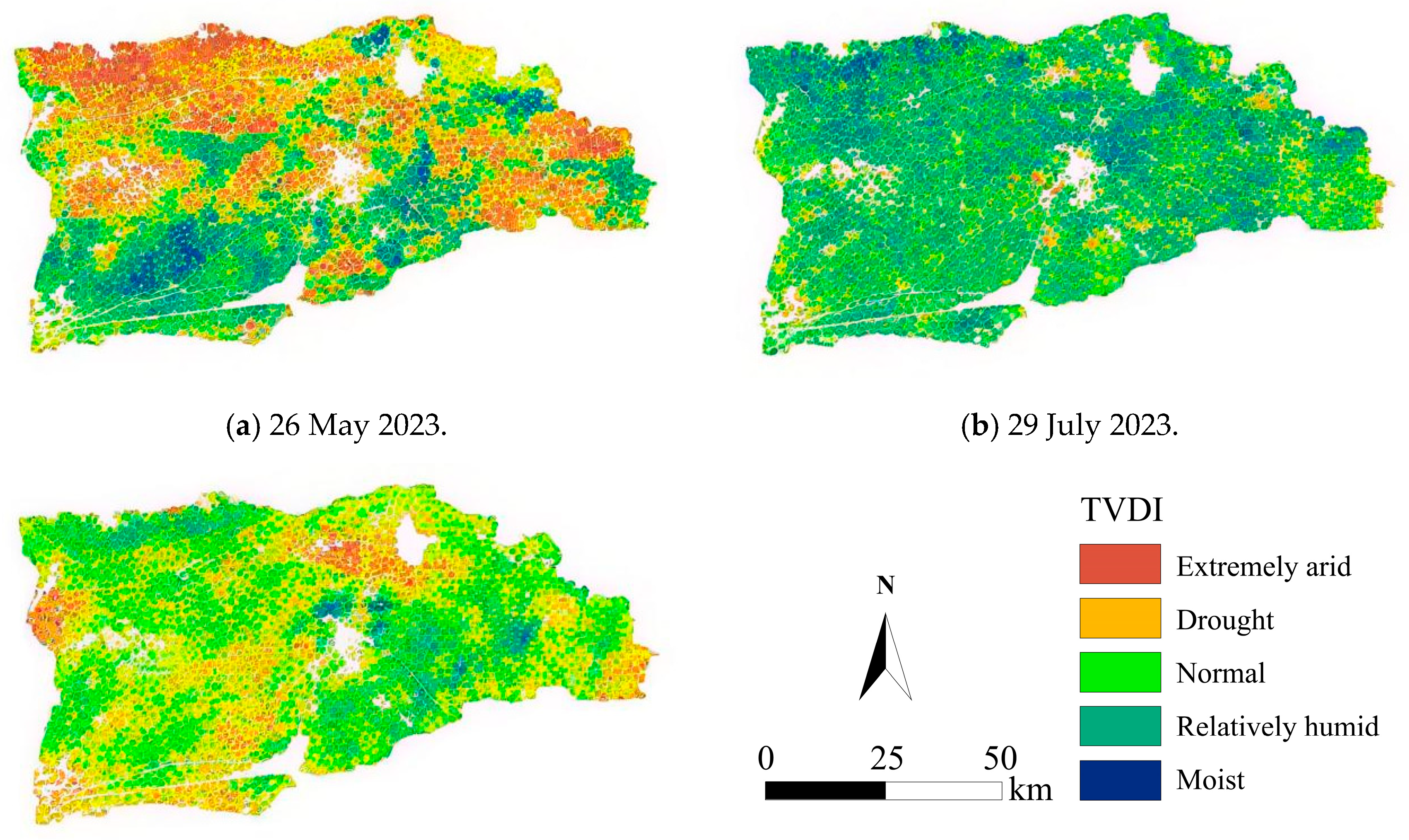
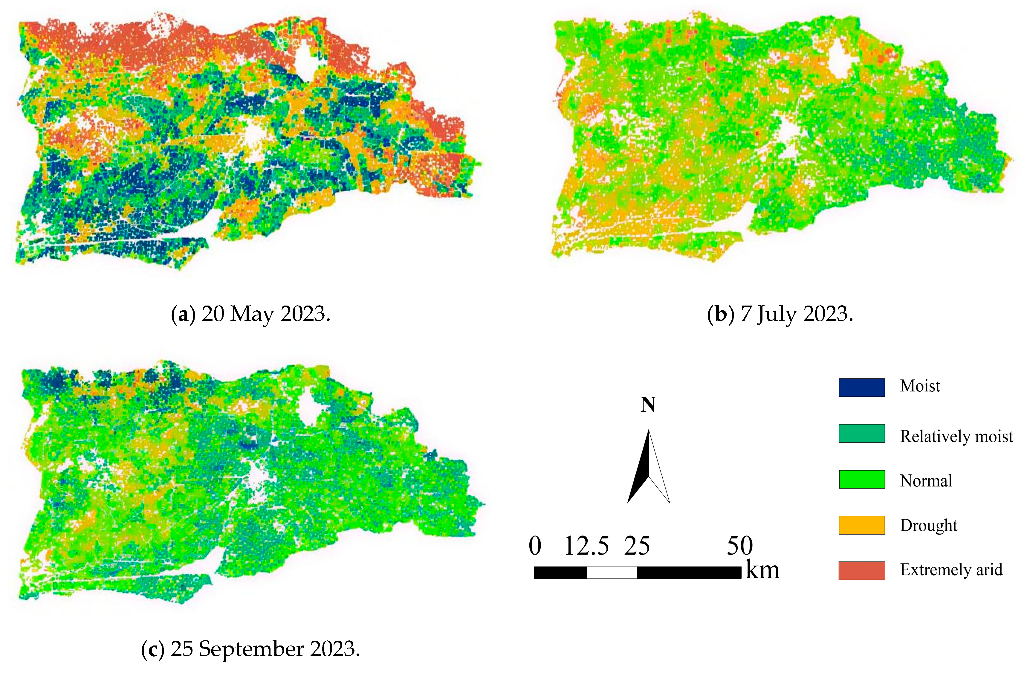
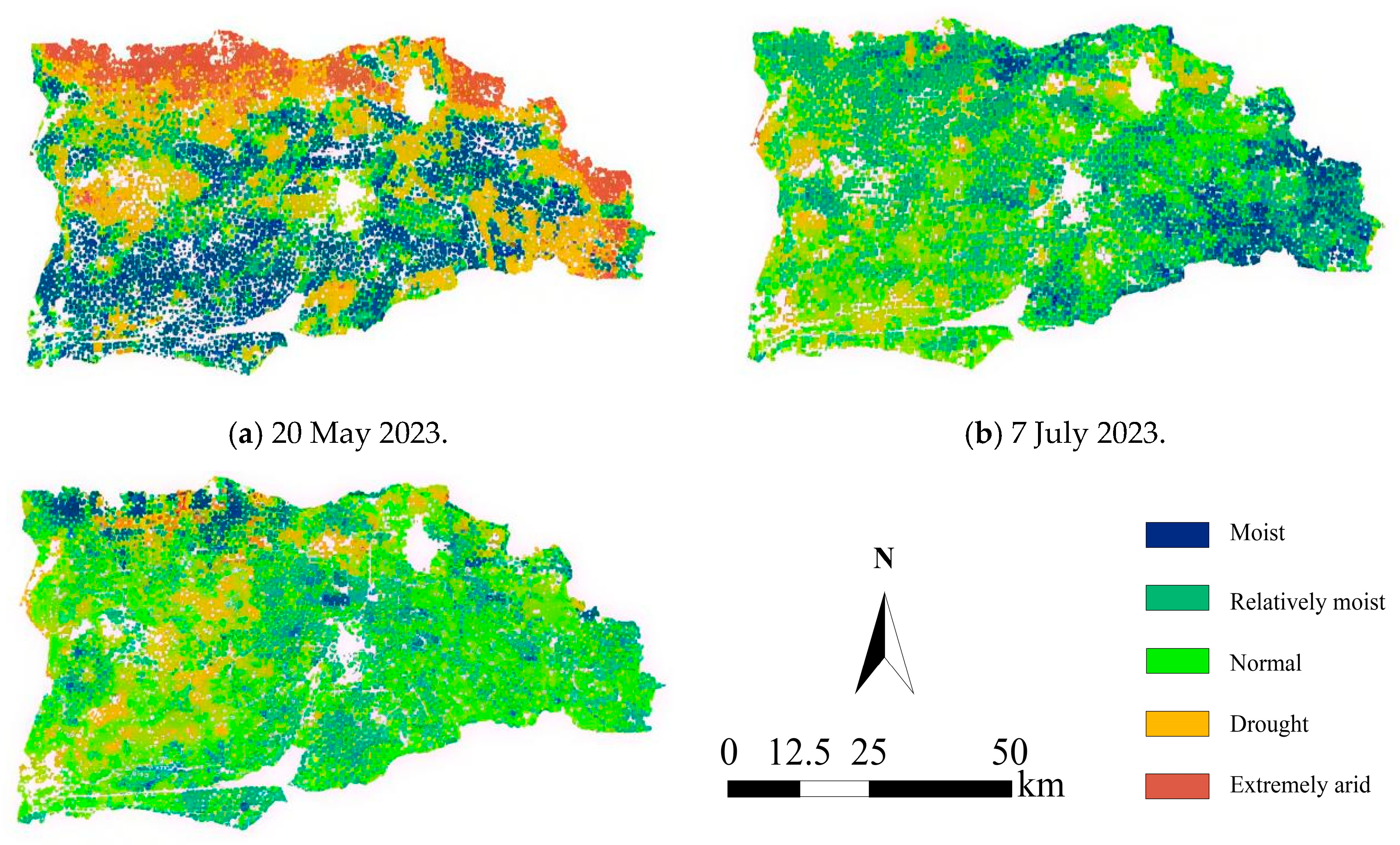
With the use of the above method to fit the dry–wet boundary equations, the TVDI corresponding to the crop growth period can then be calculated according to Equation (13). A total of 28 TVDI distribution maps were obtained for the study area in May–September 2023 and 2024, constructed using LST-NDVI and LST-EVI, respectively, a total of 28 TVDI maps were produced for May–September 2023–2024 using LST–NDVI (Figure 10 and Figure 11). To more intuitively analyze the spatial distribution and changes in soil moisture across multiple periods within the study area, the TVDI values calculated using LST-NDVI were divided into five categories, namely, 0–0.2, 0.2–0.4, 0.4–0.6, 0.6–0.8, and 0.8–1.0, corresponding to soil moisture drought levels of moist, moderately moist, normal, dry, and extremely dry, respectively.

3.2.2. Spatiotemporal Distribution of Soil Moisture Based on the LST-EVI Feature Space

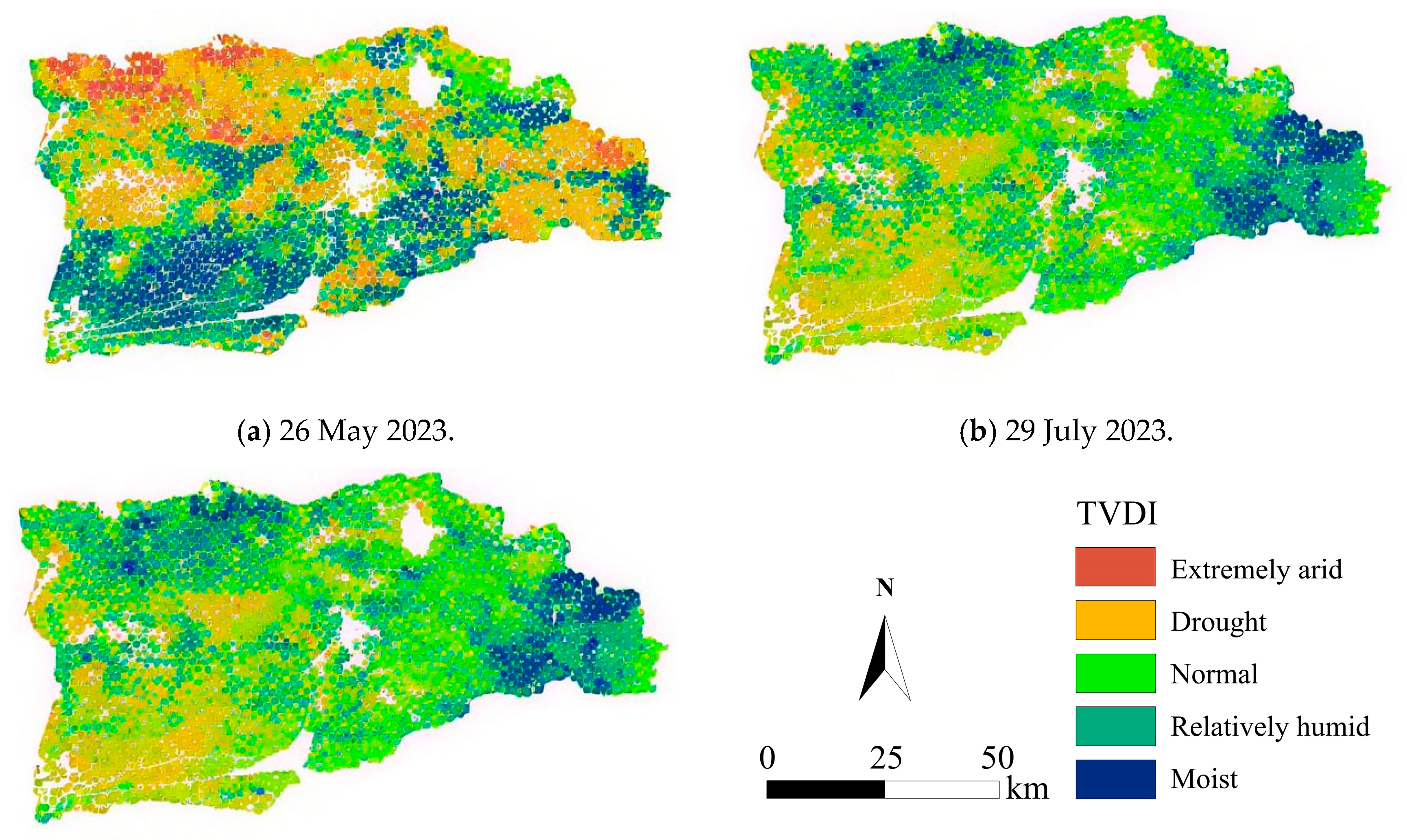
Similarly, LST–EVI-based TVDI maps were categorized into five classes, as shown in Figure 12 and Figure 13.
Figure 10, Figure 11, Figure 12 and Figure 13 display TVDI spatial distribution for 2023–2024 based on NDVI and EVI. Spatiotemporal changes are similar, so they are analyzed together. From 26 May to 11 June 2023, and from 20 May and 13 June 2024, soil moisture decreased from south to north. Before 11 June, the north remained dry/extremely dry despite the Fengji Canal, as groundwater drip irrigation caused distinct spatiotemporal patterns. Evaporation and seepage reduced moisture, becoming uniform by late June, sufficient for crops. In the northwest, drip irrigation expanded the moist areas. On 5 July 2023, the east had moist soil, with variations due to the Yichang Irrigation Basin’s large span. In the west, precipitation was similar to that in the river areas, and the east has a climate like that of Wulate Qianqi. From late July to August, the soil was moist/relatively moist during peak rainfall. By 22 August 2023, most farmland dried due to insufficient water. In September, crop maturity weakened transpiration, the soil was exposed, precipitation decreased, there was no external water input, and moisture declined.

3.2.3. Accuracy Validation and Evaluation of the TVDI Model

Accuracy validation involved linear fits of TVDI (from NDVI and EVI) against soil moisture at 0–10 cm, 10–20 cm, and 20–40 cm for 2023–2024. In 2023, R2 values were 0.478 and 0.49 for 5 July and 22 August, respectively. For 2024, R2 ranged from 0.41 to 0.57 (0–10 cm), 0.36 to 0.52 (10–20 cm), and 0.2 to 0.56 (20–40 cm). Accuracy varied by date and depth: highest at 20–40 cm on 20 May, but usually highest at 0–10 cm; 20–40 cm outperformed 10–20 cm on 20 May and 25 September; while 10–20 cm was better on 21 June and 16 August. Irrigation on 20 May 2024, caused scattered data points. TVDI showed a significant negative correlation with soil moisture, decreasing as moisture increased.
For EVI-based TVDI validation, R2 values were higher than NDVI-based validation in 2023 (0.58 and 0.62 for July and August). In 2024, R2 ranged from 0.49 to 0.74 (0–10 cm), from 0.42 to 0.48 (10–20 cm), and from 0.34 to 0.55 (20–40 cm). Accuracy was highest at 0–10 cm on 20 May, similar at 0–10 cm and 10–20 cm on 21 June, but poor at 20–40 cm, high on 16 August (R2 0.45–0.62), and lower on 25 September (0.36–0.57). Correlation was best at 0–10 cm. TVDI based on EVI had better correlation than NDVI-based TVDI, making it more suitable for soil moisture and drought analysis in the Yichang Irrigation District; thus, it was used for spatiotemporal inversion.

3.3. Soil Moisture Inversion During the Crop Non-Growing Season (Spring Irrigation and Autumn Watering)

3.3.1. Feature Parameter Selection

Referring to previous studies, sensitive influential factors for soil moisture were extracted, and feature parameters were selected from radar and optical data. A total of 18 feature parameters were used: 8 radar parameters (VV, VH, VV + VH, VV − VH, VV × VH, VV/VH, α, H) and 10 optical parameters (RED, NIR, SWIR1, SWIR2, LST, NDVI, RVI, NDII, MSI, FVI).
To utilize polarized SAR data, polarization parameters were derived from intensity-phase analysis and decomposition. Scattering parameter sensitivity relates to dielectric properties. With the use of ENVI 5.6, VH and VV channels were extracted; and additive, subtractive, multiplicative, and divisive combinations were constructed to form a composite feature space enhancing nonlinear associations while retaining original data.
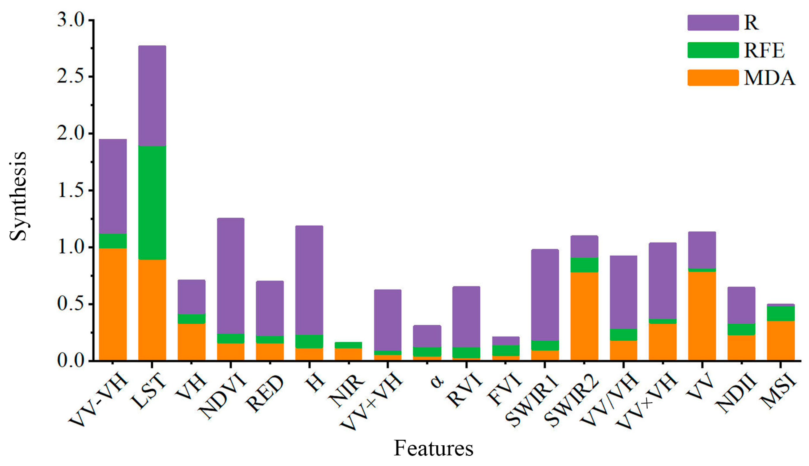
Complementary feature selection improves soil moisture inversion accuracy and efficiency. Eighteen features were ranked via RFE, MDA, and correlation analysis (normalized), yielding:
LST > VV − VH > NDVI > H > VV > SWIR2 > VV×VH > SWIR1 > VV/VH > VH > RED > RVI > NDII > VV + VH > MSI > α > FVI > NIR (Figure 14).
-
LST scored highest.
-
Optical bands: SWIR exhibited the strongest sensitivity, followed by RED, then NIR.
-
Vegetation indices: NDVI > RVI > NDII > MSI > FVI.
-
Microwave: VV outperformed VH.
-
Combined features: VV − VH ranked 2nd; VV×VH and VV/VH were intermediate; VV + VH was lowest.
-
Polarization decomposition: entropy (H) ranked high, while the average scattering angle (α) was moderate.
SWIR1/SWIR2 (1.4–1.9 μm, 1.9–2.7 μm) are moisture-sensitive. Radar cross/same-polarization combinations (e.g., VH + VV, VH × VV) provide superior sensitivity: bulk scattering dominates VH amplitude, surface scattering dominates VV, and VH has weak penetration affected by low moisture. Combinations outperform single/ratio parameters.

3.3.2. Model Construction, Inversion, and Accuracy Verification

We constructed PLSR, RF, XGBoost, and CNN models by first extracting radar–optical features and then selecting the top 10 via the procedure above. In situ datasets from 11 campaigns in 2023–2024 (N = 567) were used; data were split 70%/30% into training and test sets. Model performance was evaluated using R2, RMSE, and MAE. The evaluation indicators of the model are shown in Table 4. To minimize surface-water interference, we masked water bodies with MNDWI > −0.2 before inversion. RF, XGBoost, and CNN were trained and predicted pixel-wise in Python 3.12.4 (Python Software Foundation, Wilmington, Delaware, USA); the PLSR equation was exported for ENVI-based mapping.
Accuracy evaluation shows that, for the training set and test set, CNN > XGBoost > RF > PLSR; i.e., CNN performs best, and PLSR has the lowest accuracy. The April inversion results are better than those of October because straw residues interfere with soil moisture inversion in October, while the bare surface in April is conducive to remote sensing inversion.
We train the PLSR model in Python and print the regression equation. We use band math in ENVI to calculate the soil moisture distribution map. We train and predict RF, XGBoost, and CNN models on the Python platform to achieve pixel-by-pixel soil moisture inversion and mapping. To exclude surface water interference, we use the MNDWI index to extract water bodies (threshold MNDWI > −0.2), harvest the crops in the remaining area, and monitor the water content using the CNN model. MNDWI is an improved version of NDWI based on the green band and shortwave infrared. A value close to 1 indicates water bodies. The formula for MNDWI is expressed by Equation (18):
MNDWI = Green     SWIR Green   +   SWIR
In the formula, Green refers to the green wavelength band, and SWIR refers to the short-wave infrared wavelength band.
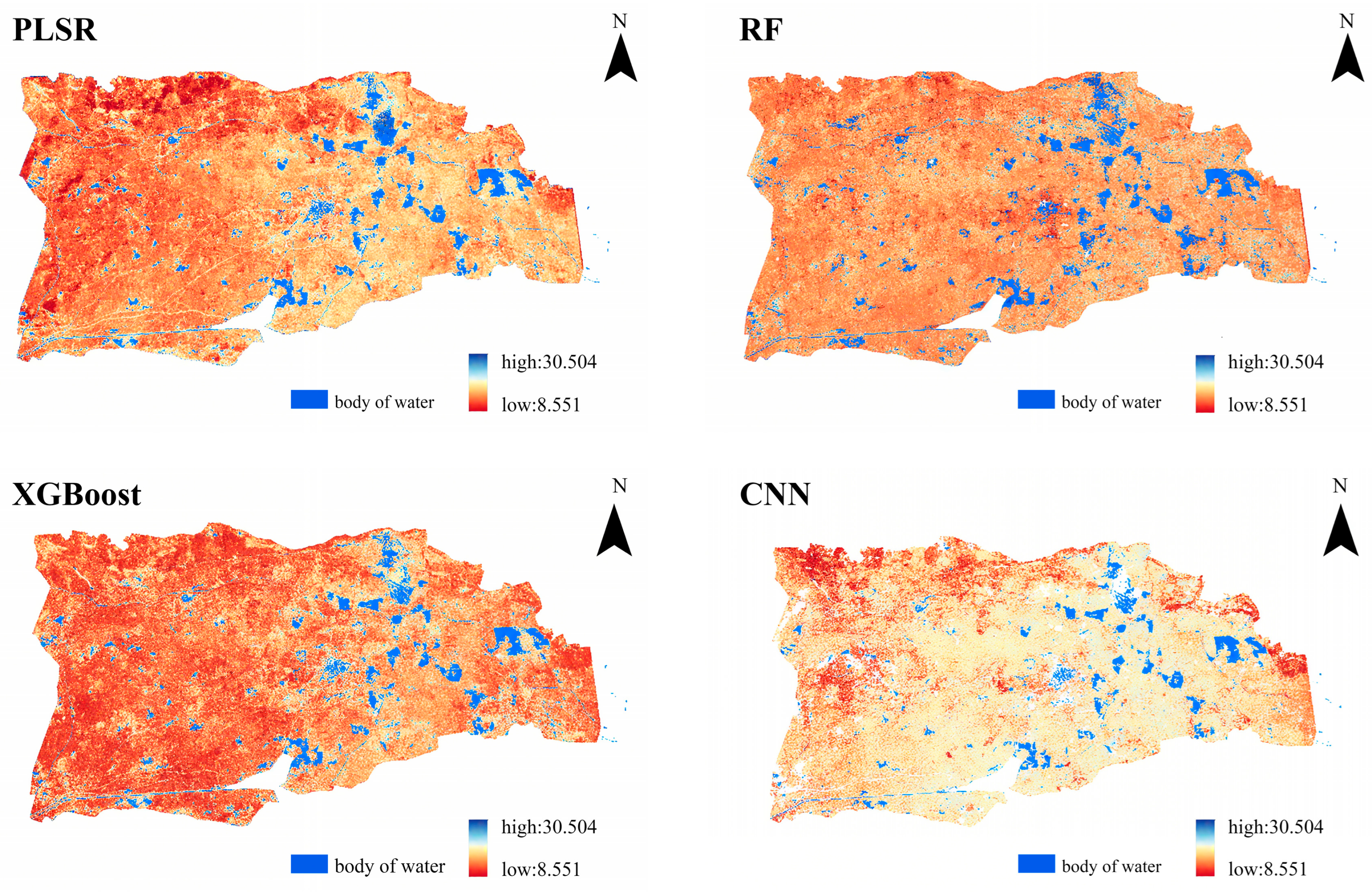
Figure 15 and Figure 16 show the soil moisture distribution maps inverted by the PLSR, RF, XGBoost, and CNN models on 15 April 2023, and 30 October 2024. The inversion results of the models are similar: PLSR has strong continuity but weak pixel-scale characterization, and RF, XGBoost, and CNN perform pixel-by-pixel inversion with high differential accuracy. CNN inversion is more precise, so the trained CNN model is used to invert the soil moisture distribution during the spring flood and autumn irrigation periods in the Yizhang irrigation area.

3.3.3. Spatial Distribution of Soil Moisture Based on CNN Model Inversion

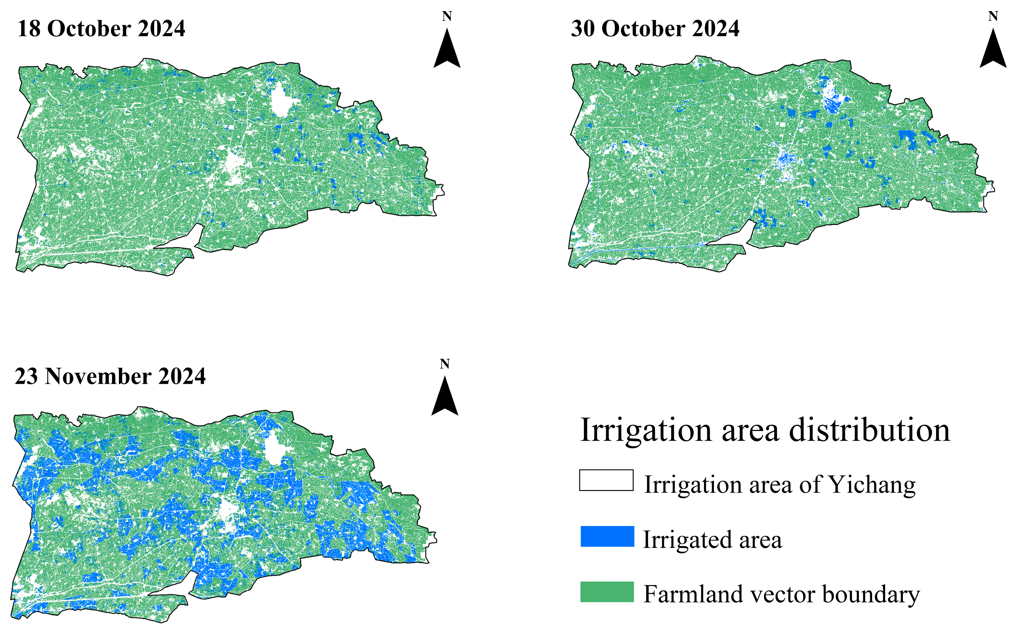
To minimize cloud interference, spring irrigation periods were 15 April, 27 April, and 21 May 2023; autumn periods were 18 October, 30 October, and 23 November 2024. A CNN model used satellite imagery from these dates to infer soil moisture distribution. Figure 17 and Figure 18 show the soil moisture distribution patterns for 2023 and 2024, respectively.
Significant spatial differences occurred in April. On 15 April, dry areas were concentrated in western/northern regions, and moist areas were concentrated in central/eastern regions. Surface water accumulated downstream in the Yihe district and upstream in the Tongji district, partly from melting autumn ice and spring irrigation, with evaporation affecting non-irrigated areas. By 27 April, irrigation increased moisture downstream in Yihe, the Zao Huo Canal, upstream in the Shahe Canal, and south of the main canal, with decreasing moisture near Wuyuan County. Extensive central/southern irrigation occurred during May’s flood peak. By 21 May, water levels rose in southern Yichang, increasing overall moisture, including in the north.
After the October harvests, exposed soils were dry, with only sporadic rainfall. By late November, autumn irrigation completion rapidly increased basin-wide soil moisture, especially in irrigated areas. By 18 October 2024, scattered eastern water bodies indicated early autumn irrigation. By 30 October, water bodies expanded significantly in eastern/southern areas, with an initial overall moisture increase.
November is the autumn irrigation peak, typically completed by 20 November. Concentrated water influx rapidly expanded water bodies and increased soil moisture. By 23 November, water bodies spread widely, primarily along the main canal and around Wuyuan County. In fields irrigated early, surface water had fully infiltrated deeper soil layers.

3.4. Irrigation Distribution Identification and Soil Moisture Dynamic Evolution Analysis

3.4.1. Identification of Irrigation Distribution During Crop Growth Periods

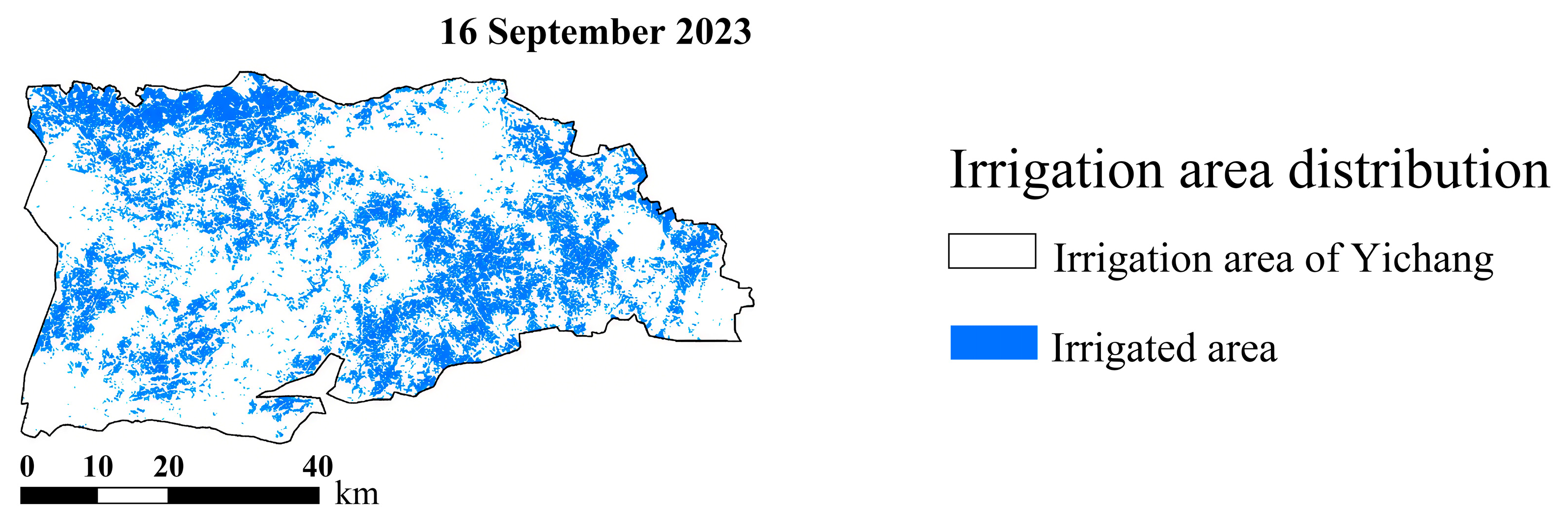
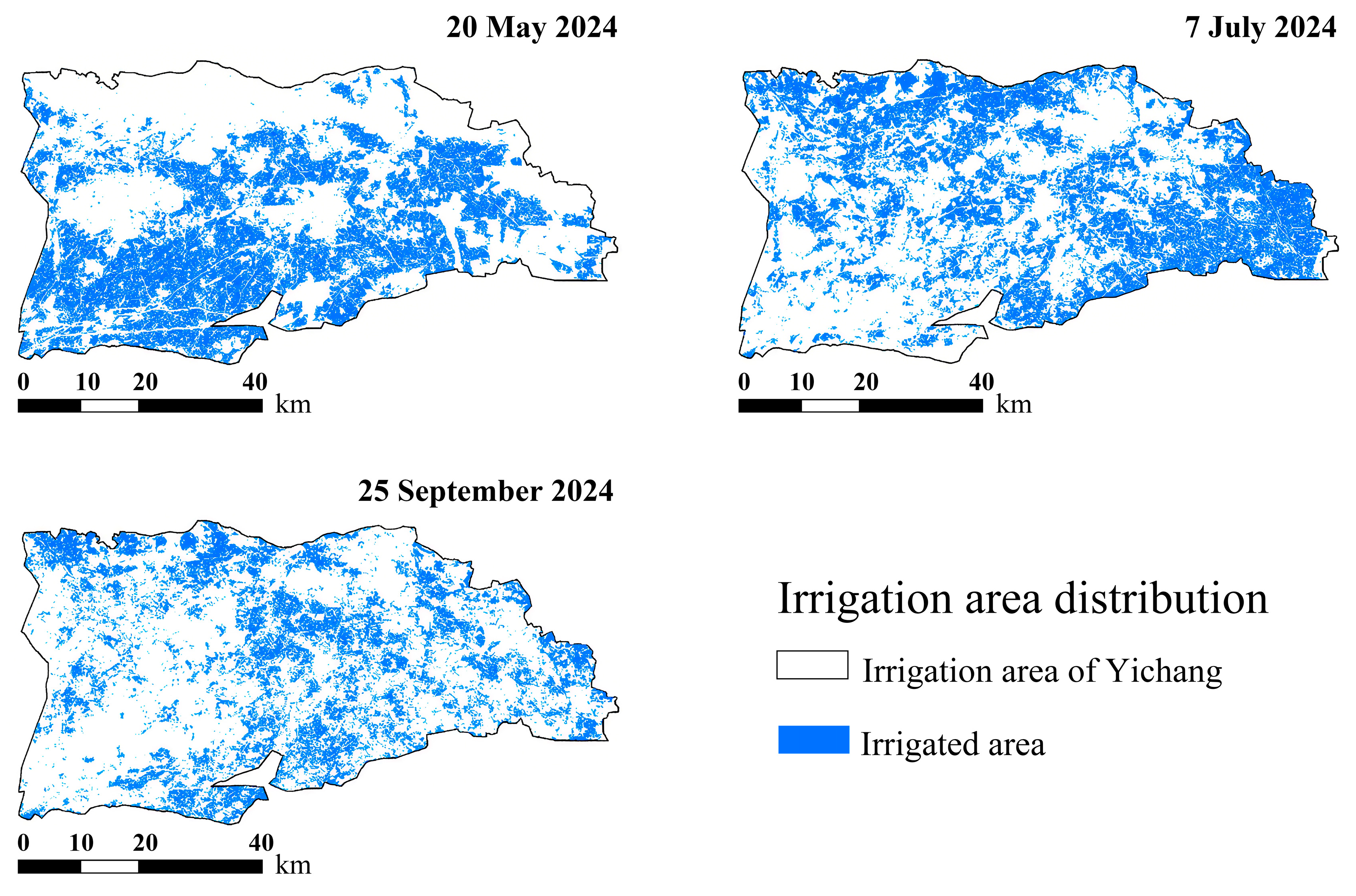
Based on the analysis and actual conditions of the Yichang irrigation area, TVDI values were divided into five levels (0–0.2, 0.2–0.4, 0.4–0.6, 0.6–0.8, 0.8–1.0), corresponding to soil moisture contents of >30, 20–30, 10–20, 5–10, and 0–5%, respectively. Irrigated farmland areas for 2023 and 2024 were extracted using a TVDI threshold of 0.4 (TVDI < 0.4 indicates irrigation). By combining this information with farmland vector data, the spatiotemporal distribution of irrigated farmland in the Yichang irrigation basin was obtained (Figure 19 and Figure 20), and the corresponding area statistics are given in Table 5.
At the pixel level, an irrigation state is defined as follows: during the growing season a pixel is classified as irrigated when TVDI < 0.4, and during the non-growing season when SMC > 20% (thresholds justified above). An irrigation event is a transition from the non-irrigated state (0) to the irrigated state (1) between two consecutive analysis scenes of the corresponding workflow (Landsat-based TVDI in the growing season; SAR–optical soil-moisture inversion in the non-growing season). To isolate irrigation from rainfall-driven wetting, a transition is attributed to irrigation only when the 3-day cumulative precipitation centered on the acquisition dates is <10 mm; otherwise, it is flagged as rainfall-driven and excluded from event counts. After classification, a small morphological opening (2 pixels) is applied to suppress speckle, and isolated single-pixel transitions that do not persist to the next scene are removed.
From late May to June, 2023, irrigation occurred in the southwestern, southern, central, and northeastern regions, covering over 100,000 ha—30% of the total area—for the spring irrigation of sunflowers and corn. Spring irrigation ended in late May, ceasing irrigation. By mid-June, soil moisture decreased, dropping to 70,000 ha by 11 June. Full-scale irrigation began in late June. In early July, irrigation in northern and eastern regions covered 100,000 ha by 5 July, which is 36% of the total area. Northern mountainous areas used groundwater drip irrigation, creating an independent spatial distribution. This supplemented areas that were not irrigated during the May–June spring flood. From July to August, concentrated precipitation and irrigation covered over 200,000 ha, which is 70% of the total area. Overlapping precipitation and irrigation maintained soil moisture, interfering with monitoring and resulting in a larger monitored area. Irrigation ceased in late August. In September, the irrigated area decreased and dispersed, dropping to 106,720 ha by 16 September.
On 20 May 2024, the irrigated area was 0.13 million ha, up year-on-year. After late May water suspension, it fell to 9698 ha on June 21. It rebounded to 0.13 million ha by 5 July, increased through July and August, exceeding 3 million mu on 16 August, then declined in September to 0.094 million ha on 25 September.
The 2023 and 2024 irrigation progress was similar, with identical change patterns. The Hetao Irrigation District conserved water, reducing autumn irrigation use from 1.6 billion m3 to less than 1 billion in 2023. The Yichang Irrigation District drew 275.75 million m3 for autumn irrigation, down 285.45 million year-on-year. The autumn irrigation area decreased in 2023, increasing the amount of dry land and leading to a rise in the 2024 spring flood irrigation area.

3.4.2. Identification of Irrigation Distribution During the Non-Growing Season of Crops

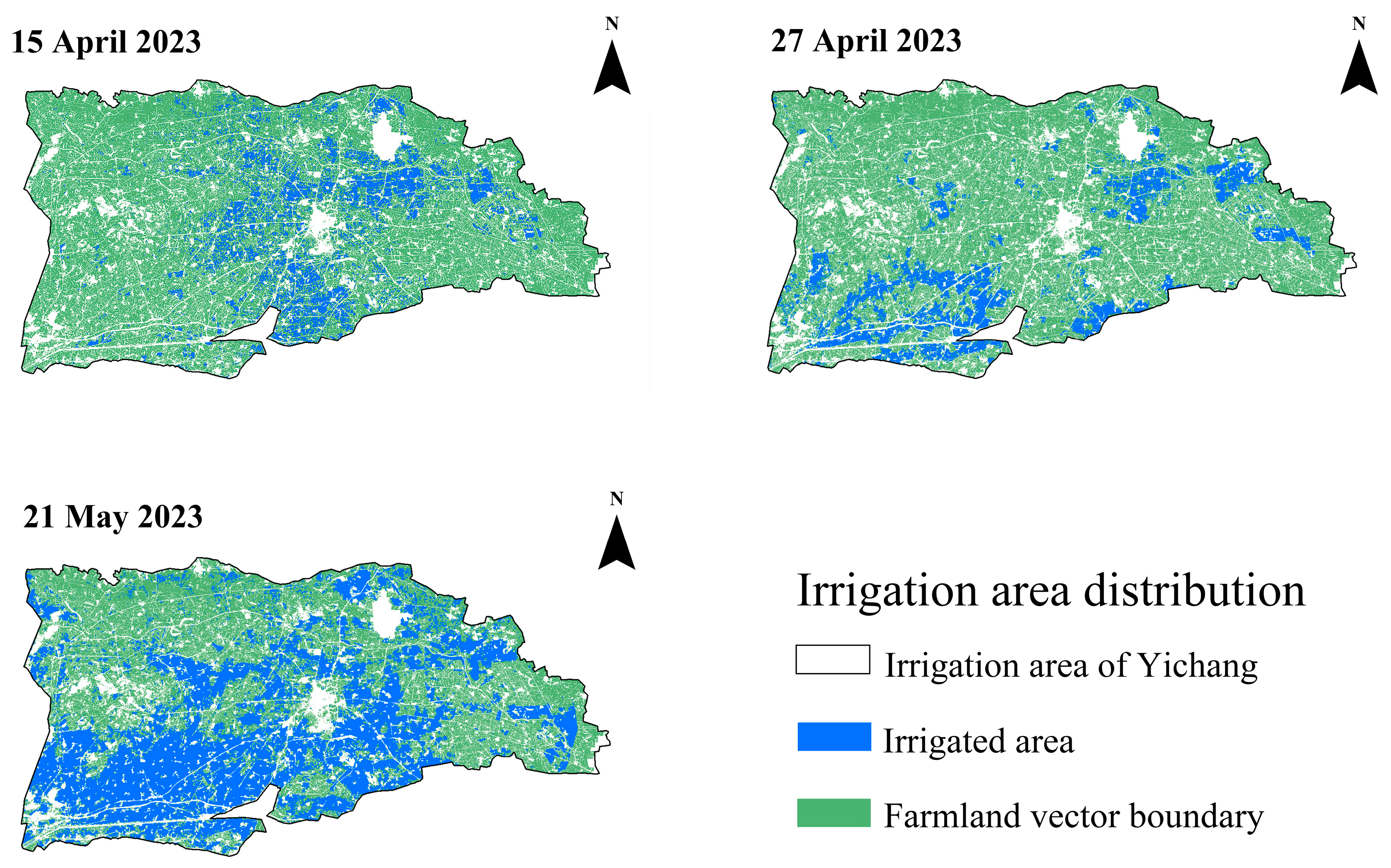
During the non-growing season, irrigation identification relies on the CNN-predicted soil-moisture maps; pixels are classified as irrigated when SMC > 20%. The TVDI-based criterion (TVDI < 0.4) applies only to the growing season. A map of the irrigation areas during this season (Figure 21, April–May, 2023) reveals the following: on 1 April, 039,833 ha irrigated around Wuyuan County, the Yihe Irrigation District, and the Tongji Irrigation District’s upper reaches, influenced by autumn irrigation and spring runoff. On 1 April, 837,058 ha irrigated Yihe’s middle-lower reaches, Zaohuo and the Shahe Main Canal’s upper reaches, and the Main Canal’s south side for easy water diversion. On 21 May, the peak reached 122,683 ha (over 40% total), with large-scale irrigation in Yichang Irrigation District’s southern and northwestern regions, significant increases around Wuyuan County, and nearly full irrigation in the southwest. The identification of irrigation events follows the definition in Section 3.4.1 (state transition between consecutive scenes with rainfall exclusion).
Figure 22 displays the spatial distribution of irrigated areas in October–November, 2024 and Table 6 presents statistics on irrigated areas during the non-fertile period of crops. Autumn irrigation, a traditional system in the Hetao Irrigation District for salt leaching and entropy conservation, began in late October, starting in the northeast. On 18 October, the irrigated area was 7651 ha, rising to 19,096 ha by 30 October and gradually expanding. It concluded in late November, reducing soil moisture. By 23 November, irrigation was concentrated in the northern Yichang Irrigation District, around Wuyuan County, and the southeast, covering 71,836 ha—over 20% of the total. Compared to spring flooding, autumn and spring irrigation spatially complement each other: fields not irrigated in autumn are irrigated in spring. In the northeast, autumn irrigation is followed by spring flooding, with overlap due to heavy saline–alkali land requiring repeated irrigation for salt leaching and crop growth.

3.5. Analysis of the Dynamic Evolution of Irrigation in the Yichang Irrigation District

3.5.1. Irrigation Progress in the Yichang Irrigation Area

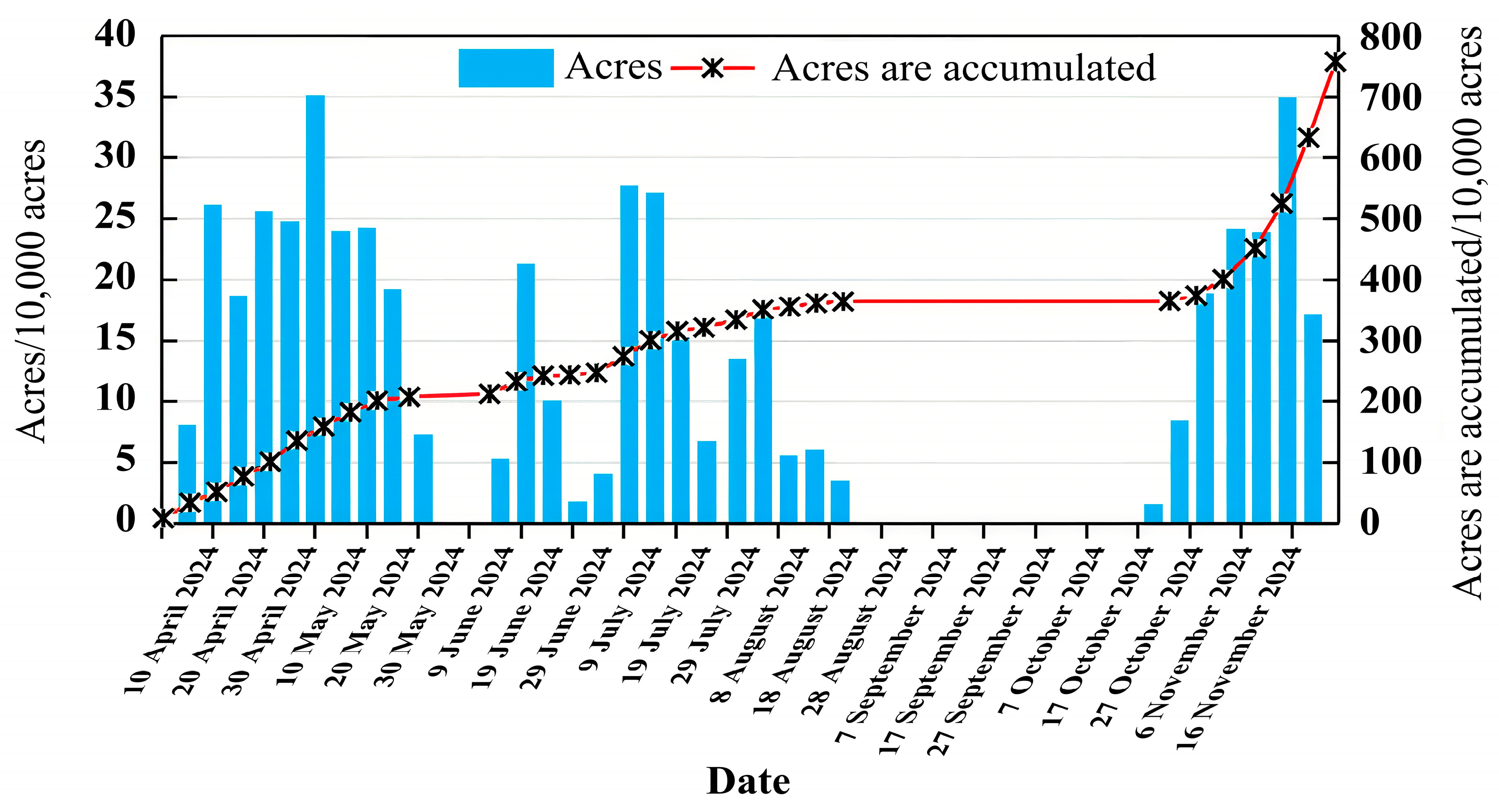
The irrigation calendar in the Yichang Irrigation District comprises three stages: spring flood irrigation (April–June), mid-season/growing-season irrigation (July–August), and autumn irrigation (October–November). The opening of the gates of the North Main Canal at the Huanghe Sanshenggong Water Conservancy Hub marks the start of spring and summer irrigation in the Hetao Irrigation District. Within 2–3 days of the gates being opened, water reaches the Yichang Irrigation District, and full-scale irrigation begins. Figure 23 shows the irrigation progress for 2024.
In April, dry fields and corn fields are irrigated to replenish soil moisture. May sees the first and second irrigation events of wheat, the arrangement of the water supply for dry fields and hot water fields, and sowing. From late May to mid-June, there is an irrigation window period with no large-scale irrigation. In late June, we have the third irrigation event for wheat and young crops such as corn, gourds, and tomatoes. In July to August, key crops such as corn and sunflowers are irrigated. Irrigation ceases in late August and resumes in October. From mid-to-late October to late November, autumn irrigation is conducted, a traditional practice in the Hexi Irrigation District. Post-harvest flood irrigation is used to leach salts and conserve moisture, accounting for one-third of annual water use, with positive benefits.

3.5.2. Comparison of Farmland Irrigation Area Identification Results with Statistical Data

We verified the accuracy of irrigation distribution identification by comparing remote sensing inversion data with statistical irrigation data for the Yichang Irrigation Basin in 2024. Due to the difficulty in matching the time periods, key dates were selected for comparison. The results are shown in Table 7.
On 20 May, during the peak period of spring irrigation, the identified irrigation area was 127,528 ha, with a calculated area of 121,120 ha, achieving an accuracy rate of 95.40%. On 16 August, at the end of the autumn irrigation period, the accuracy was 86.91%. On 23 November, at the end of the autumn watering period, the accuracy was 86.36%. The remotely sensed area was close to the calculated area. The previous year’s autumn watering helped retain soil moisture, resulting in a larger identified area during the spring flood period; however, after irrigation, during the autumn irrigation and autumn watering periods, moisture levels decreased, leading to the identification of an area that was lower than the cumulative area.

3.5.3. Analysis of Dynamic Changes in the Irrigation Area

In the Yichang Irrigation District, sunflowers constitute roughly 50% of the cropping area, corn about 30%, vegetables and fruits around 10%, and wheat about 5%. Wheat is typically sown in late March, relies on moisture from autumn irrigation, and generally requires only two irrigation events during its growth. Sunflowers are usually irrigated once before sowing and then 0–2 times during the growing season, and saline-alkali soils are flushed in autumn to reduce salt accumulation. Corn may be planted after an autumn irrigation or a spring flood; conventionally irrigated cornfields receive three to four irrigation events during the growing season, whereas drip-irrigated cornfields bypass spring and autumn flooding and instead receive about nine smaller irrigation events to meet crop water needs. These crop-specific irrigation schedules reflect local agricultural practices and water-saving guidelines.
Figure 24 illustrates irrigation area changes in the Yichang Basin from 2023 to 2024: the area increases in April, peaks near 133,400 ha in late May, declines after spring flood to below 10% in mid-June, rebounds in late June to over 30% in early July, peaks at over 200,100 ha (nearly 70%) in late July–August, and decreases in September; autumn irrigation then surges to over 66,700 ha in late October.
Spring flood irrigation serves corn and sunflower areas, with high water volumes in the south and Wuyuan County. Mid-June to early July saw no Yellow River diversion; irrigation included the spring flood and a groundwater drip. July–August irrigation involved the Yellow River and a groundwater drip, but the precipitation caused may be overestimated and obscure the impact distinction. September precipitation led to an area decrease post-irrigation. Autumn irrigation targeted corn fields, wheat fields, and saline–alkali regions.

4. Discussion

This study presents a comprehensive framework for monitoring agricultural soil moisture dynamics and irrigation patterns using multi-source remote sensing data in the Hetao Irrigation District. The key findings—notably, the superiority of EVI in constructing robust TVDI feature spaces and the efficacy of CNN in fusing radar–optical features—provide significant advancements in precision agriculture. Below, we contextualize these results within existing literature and discuss their practical implications.

4.1. Enhanced TVDI Accuracy via EVI: Mitigating NDVI Saturation

The spatiotemporal distribution of soil moisture is influenced by multiple factors, including topography, meteorological conditions, and human activities [47]. Using a single data set or one-sided information alone is insufficient to fully reflect the comprehensive status of soil moisture. The TVDI model, which combines NDVI and LST, can accurately estimate soil moisture [48] and is used to identify the spatiotemporal extent of agricultural drought and determine the severity level of drought in a specific area [49]. The LST-EVI feature space demonstrated markedly higher stability in dry-edge fitting (R2 = 0.93–0.99) compared to LST-NDVI (R2= 0.85–0.98), particularly under high vegetation coverage. This aligns with studies highlighting NDVI’s susceptibility to saturation in dense canopies ([15]). The EVI’s resistance to saturation—attributed to its built-in atmospheric correction and soil background suppression—enabled more linear responses to vegetation–water stress gradients ([13]).
By applying the TVDI model to precise farmland areas, interference from other surface vegetation cover can be eliminated, leading to more accurate assessments of changes in the characteristic space and wet–dry boundary features, as well as of the causes of these changes. This will provide guidance and reference for future research. The timely and accurate monitoring of farmland soil moisture and prompt measures in drought-affected areas are essential to maintain appropriate soil moisture levels and ensure normal crop growth. Changes in the surface vegetation cover determine the dry–wet boundary characteristics. Higher vegetation cover typically indicates faster evapotranspiration rates, and under drier conditions, evapotranspiration plays a more pronounced role in lowering surface temperatures. Cheng Z. et al. [50] constructed a TAM-Net deep learning network in the northwestern arid region, integrating the Table Diffusion Algorithm (TabDDPM), hybrid attention mechanism, and multi-task learning. Using drone-based multi-source data (spectral/thermal, infrared/texture), the authors simultaneously monitored moisture indicators, such as corn equivalent water thickness (EWT) and stomatal conductance (Gs), and generated the Fuzzy Comprehensive Water Index (FCWI), which can precisely distinguish between different irrigation gradients. However, it has only been validated for a single crop (corn), and the high cost of high-frequency UAV data limits its application in large-scale areas. Our results extend the work of Chen et al. (2021) [51] in Fujian by quantitatively validating EVI’s advantage in temperate, arid zones using high-temporal-resolution Landsat-8/9 synergy. At the same time, it has a lower cost and can be applied over a wide area. Indeed, we found that TVDI’s correlation was strongest for the 0–10 cm soil layer (R2 up to 0.74) and weaker for deeper layers, consistent with surface temperature–vegetation signals primarily reflecting topsoil moisture. Correlation strengths varied across dates, likely due to differences in rainfall or irrigation timing and crop conditions; for example, early-season observations (with lower canopy density) showed higher R2 than late-season observations under dense canopy. We also note that the TVDI threshold of 0.4 (used here to classify irrigated areas) corresponds to roughly 20% volumetric moisture. Future work could apply ROC analysis to refine this cutoff and improve irrigation-detection accuracy.

4.2. CNN-Driven Fusion of Multi-Source Features: Capturing Nonlinear Interactions

The CNN model outperformed PLSR, RF, and XGBoost in soil moisture inversion during non-growing seasons, achieving test R2 values of ≈0.61 (April) and ≈0.56 (October). This superiority stems from CNN’s capacity to hierarchically extract spatial patterns from heterogeneous features (e.g., VV-VH polarization, LST, SWIR). Specifically, the integration of Sentinel-1’s H/α decomposition parameters (entropy and scattering angle) with Landsat-derived thermal/optical indices allowed the model to disentangle complex soil–vegetation–water interactions, a challenge noted in prior studies (Zhou et al., 2021 [52]; Chen et al., 2024 [53]). Our findings resonate with those of Abowarda et al. (2021) [54], who demonstrated CNN’s edge in fusing ultra-wideband radar and multispectral data, and we further establish its scalability for operational irrigation monitoring at the canal-system scale. However, the observed performance margin of the CNN over the other models was modest (e.g., test R2 ≈ 0.61 vs ≈ 0.56). These differences may lie within sampling variability and do not necessarily imply a statistically significant advantage. Moreover, CNNs require larger training datasets and computational resources and typically act as a “black box” with limited interpretability. In practice, simpler models like RF and XGBoost—while slightly less accurate—can be advantageous due to their robustness and feature-importance insights. Future work could explore temporal convolutional networks to leverage Sentinel-1’s 6-day revisit data.

4.3. Spatial Complementarity of Irrigation: Pathways for Water Optimization

Remote sensing images clearly reveal the spatial heterogeneity of soil moisture within fields, identifying areas of water stress and areas with sufficient moisture. Managers can use this information to divide fields into irrigation management units and implement variable irrigation. The identification of spatially complementary irrigation patterns between spring irrigation (April–May, concentrated in the south) and autumn irrigation (October–November, dominant in the north) offers actionable insights for water allocation. This distribution minimizes redundancy while addressing regional disparities: salt-affected northeastern fields require dual-season irrigation for leaching, while other areas benefit from staggered scheduling. Such spatial optimization can reduce water use by 15–20% (Fu et al., 2024 [55]), directly supporting Hetao’s water-saving mandate (e.g., 2023 autumn irrigation reduced from 1.6 to 1.0 billion m3). Our approach advances statistical methods (e.g., Liu et al., 2017 [56]) by providing high-resolution (30 m), temporally explicit irrigation maps validated against canal water delivery records (accuracy: 86–95%). Integrating these maps with real-time soil moisture forecasts could enable dynamic water release protocols, aligning with FAO’s call for precision water governance in arid farmlands (FAO, 2021 [57]).

4.4. Limitations and Outlook

This study analyzed surface soil moisture dynamics in the Yichang Irrigation Basin (2023–2024) using TVDI derived from Landsat-8/9 data. While integrating both satellites improved temporal resolution, rapid farmland changes and cloud/shadow contamination during overpasses hindered continuous irrigation monitoring. To address this, future work should undertake the following:
(1)
Adopt microwave–optical synergistic inversion by coupling Sentinel-1 SAR data (cloud-penetrating) with Landsat thermal bands, using spatiotemporal fusion models (e.g., improved AIEM) and rainfall correction factors to mitigate precipitation interference.
(2)
Deploy UAV multispectral/TIR sensors during critical growth stages to achieve 3 m resolution gap-filling, supplemented by high-frequency satellites (e.g., GF-1/6, PlanetScope) for 3–5 day revisits.
(3)
Ensure near-contemporaneous SAR–optical acquisitions. In this study, Sentinel-1 and Landsat scenes for the non-growing season were matched within ≤3 days (median ≈ 2 days), which did not introduce noticeable differences. Longer gaps can bias retrievals because soil moisture changes rapidly; future work should quantify the sensitivity of moisture estimates to time offsets and, when possible, keep SAR–optical pairs within 1–2 days or apply time-series fusion to correct larger offsets.
Regional variability limited TVDI’s adaptability. Future models should undertake the following:
(1)
Implement dynamic zonal modeling by partitioning hydrological response units (HRUs) based on soil texture (clay/sand ratio), topography, and crop type, integrating covariates like surface roughness (SSR) to enhance robustness.
(2)
Expand feature engineering by incorporating MSAVI (to suppress bare soil noise) and FVC (to quantify canopy shading), fusing thermal indicators (e.g., diurnal temperature range (DTR) and canopy–air temperature difference (CATD)), and extracting phenophase-sensitive features (e.g., the EVI curve slope from Sentinel-2 time-series) to identify crop water-critical stages.

5. Conclusions

This study developed an integrated remote-sensing approach to characterize soil moisture dynamics and irrigation patterns in an arid agricultural region. We found that using the LST–EVI feature space yields significantly more stable TVDI retrievals than LST–NDVI: the dry-edge fit R2 under LST–EVI was ≈0.93–0.99 compared to ≈0.85–0.98 for LST–NDVI, and the correlation with surface moisture (0–10 cm) reached R2 up to 0.74. Regarding machine learning models, a CNN combining Sentinel-1 (VV/VH and textural metrics) and Landsat (LST, SWIR) features achieved the highest inversion accuracy (test R2 ≈ 0.56–0.61), modestly outperforming RF and XGBoost (≈0.51–0.53) but at greater data and computational cost. Finally, the maps of seasonal irrigation showed clear complementarity: spring irrigation covered ~42% of fields, autumn irrigation covered ~25%, and summer irrigation covered ~70%. Targeting the spring and autumn schemes (especially for salt-prone areas) can reduce water use by ~15–20%. Together, these findings demonstrate that multi-source remote sensing can precisely monitor year-round soil moisture and inform more efficient, seasonally adjusted irrigation management in arid regions.

Author Contributions

All authors contributed to the conception and design of this study. Y.S.: Conceptualization, data analysis, and manuscript drafting and revision. D.Z.: Data collection, data analysis and data interpretation. Z.M.: Conceptualization, experimental design, sample collection, and chemical analysis. S.Y.: Conceptualization, experimental design, sample collection, and chemical analysis. Q.L.: Conceptualization and manuscript review and critical revision for important intellectual content. Z.Q.: Manuscript review and critical revision for important intellectual content. All authors have read and agreed to the published version of the manuscript.

Funding

This research was jointly supported by the National Natural Science Foundation of China (No. U24A20179), the project for Construction of Leading Talents and Innovative Teams in Science and Technology in the Inner Mongolia Autonomous Region (BR22-13-12), and the “Talents Enriching Inner Mongolia” Project of the Inner Mongolia Autonomous Region of China (the team for technological innovation in solid waste resource utilization and salt–alkali land ecological restoration in the Yellow River irrigation area) and Natural Science Foundation Project of Inner Mongolia Autonomous Region (2025MS05114).

Institutional Review Board Statement

This study did not involve humans or animals.

Data Availability Statement

The original contributions presented in this study are included in the article. Further inquiries can be directed to the corresponding author(s).

Conflicts of Interest

The authors declare that they have no conflicts of interest.

Abbreviations

TVDITemperature–Vegetation Dryness Index
NDVINormalized Difference Vegetation Index
EVIEnhanced Vegetation Index
MNDWIModified Normalized Difference Water Index
SARSynthetic Aperture Radar
PLSRPartial Least Squares Regression
RFRandom Forest
XGBoostExtreme Gradient Boosting
CNNConvolutional Neural Network
GEEGoogle Earth Engine
RFERecursive Feature Elimination
MDAMean Decrease Accuracy
VSVersus

References

  1. Sohrabinia, M.; Rack, W.; Zawar-Reza, P. Soil moisture derived using two apparent thermal inertia functions over Canterbury, New Zealand. J. Appl. Remote Sens. 2014, 8, 083624. [Google Scholar] [CrossRef]
  2. He, L.; Qin, Q.; Panciera, R.; Tanase, M.; Walker, J.P.; Hong, Y. An Extension of the Alpha Approximation Method for Soil Moisture Estimation Using Time-Series SAR Data Over Bare Soil Surfaces. IEEE Geosci. Remote Sens. Lett. 2017, 14, 1328–1332. [Google Scholar] [CrossRef]
  3. Guan, H.; Huang, J.; Li, L.; Li, X.; Miao, S.; Su, W.; Ma, Y.; Niu, Q.; Huang, H. Improved Gaussian mixture model to map the flooded crops of VV and VH polarization data. Remote Sens. Environ. 2023, 295, 113714. [Google Scholar] [CrossRef]
  4. Zhang, H.; Wang, S.; Liu, K.; Li, X.; Li, Z.; Zhang, X.; Liu, B. Downscaling of AMSR-E Soil Moisture over North China Using Random Forest Regression. ISPRS Int. J. Geo Inf. 2022, 11, 101. [Google Scholar] [CrossRef]
  5. Weimann, A.; Von Schonermark, M.; Schumann, A.; Jorn, P.; Gunther, R. Soil moisture estimation with ERS-1 SAR data in the East-German loess soil area. Int. J. Remote Sens. 1998, 19, 237–243. [Google Scholar] [CrossRef]
  6. Liu, Z.; Li, P.; Yang, J. Soil Moisture Retrieval and Spatiotemporal Pattern Analysis Using Sentinel-1 Data of Dahra, Senegal. Remote Sensing. 2017, 9, 1197. [Google Scholar] [CrossRef]
  7. Santi, E.; Paloscia, S.; Pettinato, S.; Brocca, L.; Ciabatta, L.; Entekhabi, D. Integration of microwave data from SMAP and AMSR2 for soil moisture monitoring in Italy. Remote Sens. Environ. 2018, 212, 21–30. [Google Scholar] [CrossRef]
  8. Yang, Z.; Gong, J.; Wang, S.; Jin, T.; Wang, Y. Shifts bidirectional dependency between vegetation greening and soil moisture over the past four decades in China. Sci. Total Environ. 2023, 897, 166388. [Google Scholar] [CrossRef]
  9. Shahvaran, A.R.; Kheyrollah Pour, H.; Binding, C.; Van Cappellen, P. Mapping satellite-derived chlorophyll-a concentrations from 2013 to 2023 in Western Lake Ontario using Landsat 8 and 9 imagery. Sci. Total Environ. 2025, 968, 178881. [Google Scholar] [CrossRef]
  10. Wei, W.; Pang, S.; Wang, X.; Zhou, L.; Xie, B.; Zhou, J.; Li, C. Temperature Vegetation Precipitation Dryness Index (TVPDI)-based dryness-wetness monitoring in China. Remote Sens. Environ. 2020, 248, 111957. [Google Scholar] [CrossRef]
  11. Li, R.; Zhang, S.; Li, F.; Lin, X.; Luo, M.; Wang, S.; Yang, L.; Zhao, X. Impact of time-lagging and time-preceding environmental variables on top layer soil moisture in semiarid grasslands. Sci. Total Environ. 2024, 912, 169406. [Google Scholar] [CrossRef] [PubMed]
  12. Nugraha, A.S.A.; Kamal, M.; Murti, S.H.; Widyatmanti, W. Development of the triangle method for drought studies based on remote sensing images: A review. Remote Sens. Appl. Soc. Environ. 2023, 29, 100920. [Google Scholar] [CrossRef]
  13. Sandholt, I.; Rasmussen, K.; Andersen, J. A simple interpretation of the surface temperature/vegetation index space for assessment of surface moisture status. Remote Sens. Environ. 2002, 79, 213–224. [Google Scholar] [CrossRef]
  14. Tagesson, T.; Horion, S.; Nieto, H.; Zaldo Fornies, V.; Mendiguren González, G.; Bulgin, C.E.; Ghent, D.; Fensholt, R. Disaggregation of SMOS soil moisture over West Africa using the Temperature and Vegetation Dryness Index based on SEVIRI land surface parameters. Remote Sens. Environ. 2018, 206, 424–441. [Google Scholar] [CrossRef]
  15. Chen, J.; Wang, C.; Jiang, H.; Mao, L.; Yu, Z. Estimating soil moisture using Temperature–Vegetation Dryness Index (TVDI) in the Huang-huai-hai (HHH) plain. Int. J. Remote Sens. 2011, 32, 1165–1177. [Google Scholar] [CrossRef]
  16. Bai, J.-j.; Yu, Y.; Di, L. Comparison between TVDI and CWSI for drought monitoring in the Guanzhong Plain, China. J. Integr. Agric. 2017, 16, 389–397. [Google Scholar] [CrossRef]
  17. Lu, Z.; Shen, C.; Zhan, C.; Tang, H.; Luo, C.; Meng, S.; An, Y.; Wang, H.; Kou, X. Quantifying Multifactorial Drivers of Groundwater–Climate Interactions in an Arid Basin Based on Remote Sensing Data. Remote Sensing. 2025, 17, 2472. [Google Scholar] [CrossRef]
  18. Li, S.; Li, C.; Yao, D.; Wang, X.; Gao, Y. Bowl effect of irreversible primary salinization driven by geology in Hetao irrigation area, China. Sci. Total Environ. 2024, 920, 170834. [Google Scholar] [CrossRef] [PubMed]
  19. Xiang, Z.; Moriasi, D.N.; Samimi, M.; Mirchi, A.; Taghvaeian, S.; Steiner, J.L.; Verser, J.A.; Starks, P.J. SWAT-IRR: A new irrigation algorithm for soil and water Assessment tool to facilitate water management and Conservation in irrigated regions. Comput. Electron. Agric. 2025, 232, 110142. [Google Scholar] [CrossRef]
  20. Zhao, Y.; Yang, S.; Shi, H.; Han, H.; Dong, Y.; Li, X.; Yan, J.; Yan, Y.; Dou, X.; Tian, F.; et al. Analysis of soil salinization and land use change under water conservation retrofit in the Hetao irrigation district. Smart Agric. Technol. 2025, 12, 101143. [Google Scholar] [CrossRef]
  21. Huang, F.; Chunyu, X.; Zhang, D.; Chen, X.; Ochoa, C.G. A framework to assess the impact of ecological water conveyance on groundwater-dependent terrestrial ecosystems in arid inland river basins. Sci. Total Environ. 2020, 709, 136155. [Google Scholar] [CrossRef]
  22. Zhao, Y.; Miao, Q.; Shi, H.; Li, X.; Yan, J.; Yang, S.; Hou, C.; Yu, C.; Feng, W.; Hao, J. Inversion of soil salinization at the branch canal scale in the Hetao Irrigation District based on improved spectral indices. Agric. Water Manag. 2025, 316, 109608. [Google Scholar] [CrossRef]
  23. Li, J.; He, P.; Chen, J.; Hamad, A.A.A.; Dai, X.; Jin, Q.; Ding, S. Tomato performance and changes in soil chemistry in response to salinity and Na/Ca ratio of irrigation water. Agric. Water Manag. 2023, 285, 108363. [Google Scholar] [CrossRef]
  24. Miao, Q.; Rosa, R.D.; Shi, H.; Paredes, P.; Zhu, L.; Dai, J.; Gonçalves, J.M.; Pereira, L.S. Modeling water use, transpiration and soil evaporation of spring wheat–maize and spring wheat–sunflower relay intercropping using the dual crop coefficient approach. Agric. Water Manag. 2016, 165, 211–229. [Google Scholar] [CrossRef]
  25. Feng, Z.; Miao, Q.; Shi, H.; Li, X.; Yan, J.; Gonçalves, J.M.; Dai, L.; Feng, W. Irrigation scheduling in sand-layered farmland: Evaluation of water and salinity dynamics in the soil by SALTMED-1D model under mulched maize production in Hetao Irrigation District, China. Eur. J. Agron. 2024, 157, 127177. [Google Scholar] [CrossRef]
  26. Altuwaijri, H.A.; Al Kafy, A.; Rahaman, Z.A.; Fariha, J.N.; Miah, M.T.; Mishu, R.A.; Nath, H.; Sonet, M.S. Biophysical parameters and land surface temperature dynamics in arid urban environments: A comprehensive machine learning approach. Environ. Earth Sci. 2025, 84, 434. [Google Scholar] [CrossRef]
  27. Echavarría-Caballero, C.; Domínguez-Gómez, J.A.; González-García, C.; Domínguez-Perez, R.; García-García, M.J. Warming inland water in peninsular Spain revealed by landsat 5 analysis. Geocarto Int. 2024, 39, 2371923. [Google Scholar] [CrossRef]
  28. Imroah, F.F.K.; Setiawan, N. Integration of Landsat-8 OLI/TIRS and Sentinel-1A PolSAR for analyzing land surface temperature and its anomalies linked to ENSO in Surakarta, Indonesia. Geomatica 2024, 76, 100038. [Google Scholar] [CrossRef]
  29. Portela, B.; van der Werff, H.; Hecker, C.; van der Meijde, M. Landsat Next current design for geological remote sensing: VNIR-SWIR-TIR data continuity and new opportunities. Sci. Remote Sens. 2025, 12, 100258. [Google Scholar] [CrossRef]
  30. Cui, Y.; Chen, S.; Mo, G.; Ji, D.; Lv, L.; Fu, J. Snow Depth Retrieval Using Sentinel-1 Radar Data: A Comparative Analysis of Random Forest and Support Vector Machine Models with Simulated Annealing Optimization. Remote Sensing. 2025, 17, 2584. [Google Scholar] [CrossRef]
  31. Numbisi, F.N. Minding Spatial Allocation Entropy: Sentinel-2 Dense Time Series Spectral Features Outperform Vegetation Indices to Map Desert Plant Assemblages. Remote Sens. 2025, 17, 2553. [Google Scholar] [CrossRef]
  32. Mateus, P.; Nico, G.; Catalão, J.; Miranda, P.M.A. Precipitable water vapor from Sentinel-1 improves the forecast of extratropical storm Barbara. Q. J. R. Meteorol. Soc. 2024, 150, 1988–2004. [Google Scholar] [CrossRef]
  33. He, Y.; Yin, H.; Chen, Y.; Xiang, R.; Zhang, Z.; Chen, H. Soil Salinity Estimation Based on Sentinel-1/2 Texture Features and Machine Learning. IEEE Sens. J. 2024, 24, 15302–15310. [Google Scholar] [CrossRef]
  34. Freeman, A.; Durden, S.L. A three-component scattering model for polarimetric SAR data. IEEE Trans. Geosci. Remote Sens. 1998, 36, 963–973. [Google Scholar] [CrossRef]
  35. Cloude, S.R.; Pottier, E. An entropy based classification scheme for land applications of polarimetric SAR. IEEE Trans. Geosci. Remote Sens. 1997, 35, 68–78. [Google Scholar] [CrossRef]
  36. Fayyaz, A.; Waqas, M.; Asghar, H.; Ahmed, R.; Liaqat, U.; Naseem, K.; Baig, M.A. Rapid elemental imaging of copper-bearing critical ores using laser-induced breakdown spectroscopy coupled with PCA and PLS-DA. Talanta 2026, 296, 128463. [Google Scholar] [CrossRef]
  37. Breiman, L. Random Forests. Mach. Learn. 2001, 45, 5–32. [Google Scholar] [CrossRef]
  38. Chen, T.; Guestrin, C. XGBoost: A Scalable Tree Boosting System. In Proceedings of the 22nd ACM SIGKDD International Conference on Knowledge Discovery and Data Mining, San Francisco, CA, USA, 13–17 August 2016; pp. 785–794. [Google Scholar]
  39. Zhang, T.; Shen, X.; Cao, L. Terrain and individual tree vertical structure-based approach for point clouds co-registration by UAV and Backpack LiDAR. Int. J. Appl. Earth Obs. Geoinf. 2025, 139, 104544. [Google Scholar] [CrossRef]
  40. Miao, J.; Wang, J.; Zhao, D.; Shen, Z.; Xiang, H.; Gao, C.; Li, W.; Cui, L.; Wu, G. Modeling strategies and influencing factors in retrieving canopy equivalent water thickness of mangrove forest with Sentinel-2 image. Ecol. Indic. 2024, 158, 111497. [Google Scholar] [CrossRef]
  41. Rawat, K.S.; Sehgal, V.K.; Singh, S.K.; Ray, S.S. Soil moisture estimation using triangular method at higher resolution from MODIS products. Phys. Chem. Earth Parts A/B/C 2022, 126, 103051. [Google Scholar] [CrossRef]
  42. Lu, Y.; Tao, H.; Wu, H. Dynamic Drought Monitoring in Guangxi Using Revised Temperature Vegetation Dryness Index. Wuhan Univ. J. Nat. Sci. 2007, 12, 663–668. [Google Scholar] [CrossRef]
  43. Tucker, C.J. Red and photographic infrared linear combinations for monitoring vegetation. Remote Sens. Environ. 1979, 8, 127–150. [Google Scholar] [CrossRef]
  44. Carlson, T.N.; Ripley, D.A. On the relation between NDVI, fractional vegetation cover, and leaf area index. Remote Sens. Environ. 1997, 62, 241–252. [Google Scholar] [CrossRef]
  45. Huete, A.; Didan, K.; Miura, T.; Rodriguez, E.P.; Gao, X.; Ferreira, L.G. Overview of the radiometric and biophysical performance of the MODIS vegetation indices. Remote Sens. Environ. 2002, 83, 195–213. [Google Scholar] [CrossRef]
  46. Jiang, Z.; Huete, A.R.; Didan, K.; Miura, T. Development of a two-band enhanced vegetation index without a blue band. Remote Sens. Environ. 2008, 112, 3833–3845. [Google Scholar] [CrossRef]
  47. Jiang, L.; Islam, S. Estimation of surface evaporation map over Southern Great Plains using remote sensing data. Water Resources Research. 2001, 37, 329–340. [Google Scholar] [CrossRef]
  48. Nemani, R.R.; Running, S.W. Estimation of Regional Surface Resistance to Evapotranspiration from NDVI and Thermal-IR AVHRR Data. J. Appl. Meteorol. Climatol. 1989, 28, 276–284. [Google Scholar] [CrossRef]
  49. Price, J.C. Using spatial context in satellite data to infer regional scale evapotranspiration. IEEE Trans. Geosci. Remote Sens. 1990, 28, 940–948. [Google Scholar] [CrossRef]
  50. Cheng, Z.; Gu, X.; Zhang, Z.; Xu, Y.; Zhao, T.; Li, Y.; Sun, S.; Du, Y.; Cai, H. TAM-Net: A deep network combining tabular diffusion algorithm, attention mechanism, and multi-task learning for monitoring crop water status from UAV multi-source images. Eur. J. Agron. 2025, 170, 127778. [Google Scholar] [CrossRef]
  51. Chen, Z.; Huang, W.; Ye, S.; Qi, X. Analysis of Differences in Agricultural Drought Monitoring in Fujian Province in 2018 Based on Different TVDI Indices. J. Nat. Disasters 2021, 30, 233–243. [Google Scholar] [CrossRef]
  52. Zhou, S.; Williams, A.P.; Lintner, B.R.; Berg, A.M.; Zhang, Y.; Keenan, T.F.; Cook, B.I.; Hagemann, S.; Seneviratne, S.I.; Gentine, P. Soil moisture–atmosphere feedbacks mitigate declining water availability in drylands. Nat. Clim. Change 2021, 11, 38–44. [Google Scholar] [CrossRef]
  53. Chen, X.; Ding, Y.; Zheng, X.; Xu, C.; Wu, Z.; Xie, Q. Improved estimation of non-photosynthetic vegetation cover using a novel multispectral slope difference index with soil information, Sentinel-1 data, and machine learning. Ecol. Inform. 2024, 84, 102930. [Google Scholar] [CrossRef]
  54. Abowarda, A.S.; Bai, L.; Zhang, C.; Long, D.; Li, X.; Huang, Q.; Sun, Z. Generating surface soil moisture at 30 m spatial resolution using both data fusion and machine learning toward better water resources management at the field scale. Remote Sens. Environ. 2021, 255, 112301. [Google Scholar] [CrossRef]
  55. Fu, D.; Jin, X.; Jin, Y.; Mao, X. Extraction of grassland irrigation information in arid regions based on multi-source remote sensing data. Agric. Water Manag. 2024, 302, 109010. [Google Scholar] [CrossRef]
  56. Liu, Y.; Wu, W.; Li, Z.; Zhou, Q. Extracting irrigated cropland spatial distribution in China based on time-series NDVI. Trans. Chin. Soc. Agric. Eng. 2017, 33, 276–284. [Google Scholar] [CrossRef]
  57. Food and Agriculture Organization. The State of the World’s Land and Water Resources for Food and Agriculture—Systems at Breaking Point; Food and Agriculture Organization: Rome, Italy, 2021. [Google Scholar]
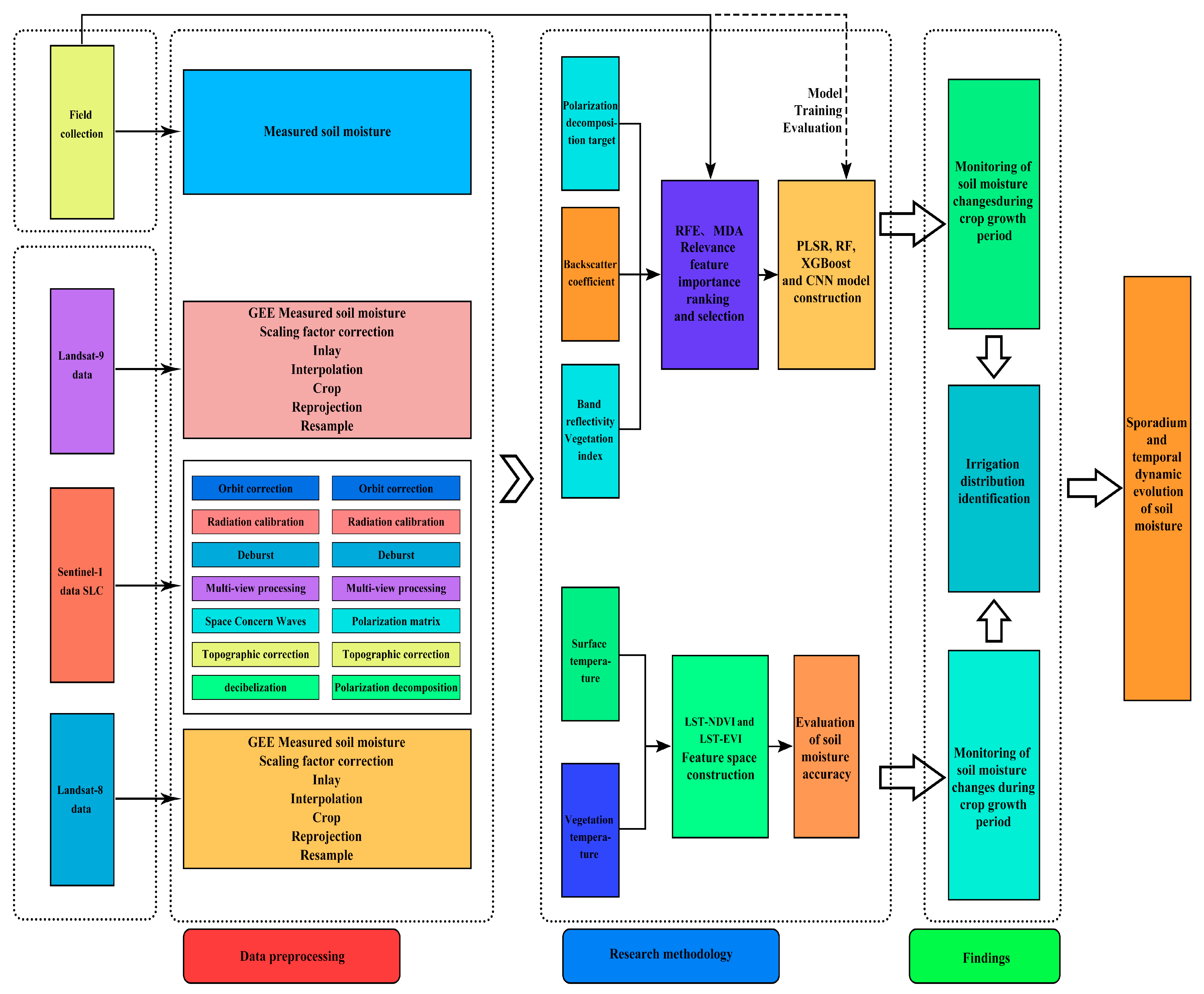
Figure 1. Technology roadmap (abbreviations: GEE = Google Earth Engine; RFE = Recursive Feature Elimination; MDA = Mean Decrease Accuracy; VIP = Variable Importance in Projection).
Agriculture 15 01946 g001
Figure 2. Overview map of the study area.
Agriculture 15 01946 g002
Figure 3. Precipitation and mean temperature for 2023 and 2024.
Agriculture 15 01946 g003
Figure 4. Convolutional neural network structure.
Agriculture 15 01946 g004
Figure 5. Schematic diagram of the full connectivity layer.
Agriculture 15 01946 g005
Figure 6. Temperature–vegetation index feature space.
Agriculture 15 01946 g006
Figure 7. Conceptual diagram of the surface temperature versus vegetation index in triangular/trapezoidal characteristic space. (Each red dot in the figure represents the measured data of a pixel or sampling point; A denotes the vertical distance from the dry side to the wet side, representing the difference between the maximum possible temperature (dry side temperature) and the minimum possible temperature (wet side temperature) under identical NDVI conditions; B denotes the vertical distance from the red dot to the wet side, representing the difference between the LST at that point and the minimum possible temperature (wet side temperature) under identical NDVI conditions; The dashed lines represent TVDI isoclines).
Agriculture 15 01946 g007
Figure 8. Temperature maxima and wet/dry edge fitting in the LST-NDVI feature space for 2023–2024.
Agriculture 15 01946 g008
Figure 9. Temperature maxima and wet/dry edge fitting in LST-EVI feature space for 2023–2024.
Agriculture 15 01946 g009
Figure 10. Spatial distribution of NDVI-based TVDI in Yichang Irrigation Domain in 2023.
Agriculture 15 01946 g010
Figure 11. Spatial distribution of NDVI-based TVDI in Yichang Irrigation Domain in 2024.
Agriculture 15 01946 g011
Figure 12. Spatial distribution of TVDI based on EVI in Yichang Irrigation Domain in 2023.
Agriculture 15 01946 g012
Figure 13. Spatial distribution of TVDI based on EVI in Yichang Irrigation Domain in 2024.
Agriculture 15 01946 g013
Figure 14. Results of adding values.
Agriculture 15 01946 g014
Figure 15. Spatial distribution of soil moisture based on different models on 15 April 2023.
Agriculture 15 01946 g015
Figure 16. Spatial distribution of soil moisture based on different models on 30 October 2023.
Agriculture 15 01946 g016
Figure 17. Soil water distribution in April–May, 2023.
Agriculture 15 01946 g017
Figure 18. Soil water distribution in October, 2024.
Agriculture 15 01946 g018
Figure 19. Spatial and temporal evolution of irrigation distribution in the Yichang Irrigation District during crop fertility in 2023.
Agriculture 15 01946 g019aAgriculture 15 01946 g019b
Figure 20. Spatial and temporal evolution of irrigation distribution in the Yichang Irrigation District during crop fertility in 2024.
Agriculture 15 01946 g020
Figure 21. Identification of spatial distribution of irrigation in April–May, 2023.
Agriculture 15 01946 g021
Figure 22. Identification of spatial distribution of irrigation, October–November, 2024.
Agriculture 15 01946 g022
Figure 23. Irrigation progress in the Yichang Irrigation District in 2024.
Agriculture 15 01946 g023
Figure 24. Irrigated area statistics for 2023 and 2024.
Agriculture 15 01946 g024
Table 1. Description of crop growth stages during the growing season. (Data source: [25]).
Crop WheatCornSunflowerZucchini
AprilEarlySowing
Mid-
LateGerminationSowing
MayEarlyTilleringSowing Sowing
Mid- Germination Germination
LateStem elongation Sowing
JuneEarly SowingFirst bloom
Mid-Spike formation First bloom
LateSpike emergenceStem elongationGerminationFruiting
JulyEarlyMilk stage Fruiting
Mid- Silking
LateMaturitySilkingBudding
AugustEarly Blooming
Mid- BloomingMaturity
Late Milk stage
SeptemberEarly
Mid-
Late MaturityMaturity
OctoberEarly Maturity
Table 2. Main parameters of Landsat-8/9.
NameBand NameBand (μm)Spatial Resolution
SR_B1Ultra-Blue0.435–0.45130
SR_B2Blue0.452–0.51230
SR_B3Green0.533–0.59030
SR_B4Red0.636–0.67330
SR_B5Near-Infrared0.851–0.87930
SR_B6Shortwave Infrared 11.566–1.65130
SR_B7Shortwave Infrared 22.107–2.29430
ST_B10Surface Temperature10.60–11.19100
Table 3. Imaging mode and parameter description of Sentinel-1 satellite.
ModeIncidence Angle (°)Resolution (m)Swath Width (km)Polarization Mode
Strip imaging (SM)20–455 × 580Single, dual polarization
Interferometric wide swath (IW)29–455 × 20250Single, dual polarization
Ultra-wide swath (EW)19–47/22–3520 × 40400Single, dual polarization
Wave (Wave)35–385 × 520 × 20Single polarization
Table 4. Model evaluation indicators.
TimeModelTraining SetTest Set
R2RMSE (%)MAE (%)R2RMSE (%)MAE (%)
AprilPLSR0.483.472.490.443.9543.281
RF0.572.561.910.533.082.48
XGBoost0.612.311.710.592.631.86
CNN0.672.301.460.612.852.22
OctoberPLSR0.453.662.860.413.933.42
RF0.523.452.710.513.442.98
XGBoost0.563.122.630.523.022.75
CNN0.612.512.430.562.642.66
Table 5. Statistics on irrigated area during crop fertility.
2023Irrigated Area (10,000 ha)Area Ratio
(%)
2024Irrigated Area (10,000 ha)Area Proportion (%)
26 May10.5436.0320 May12.7043.39
3 June10.1134.5813 June4.8416.53
11 June7.2124.6321 June0.973.31
5 July10.5336.007 July13.4345.88
22 August20.4269.7916 August20.9971.42
16 September10.6736.4725 September9.4532.29
Table 6. Statistics on irrigated area during the non-fertile period of crops.
2023Irrigated Area (10,000 ha)Area Ratio
(%)
2024Irrigated Area (10,000 mha)Area Proportion (%)
15 April3.9513.44 18 October0.772.61
27 April3.6212.36 30 October1.916.53
21 May12.2141.74 23 November7.1824.55
Table 7. Comparison of identified area and cumulative area, together with the accuracy rate.
DateIdentified Area/Million AcresCumulative Area/Million AcresAccuracy (%)
20 May 2024190.34181.5995.40
16 August 2024313.29360.4986.91
23 November 2024107.70124.7186.36
Disclaimer/Publisher’s Note: The statements, opinions and data contained in all publications are solely those of the individual author(s) and contributor(s) and not of MDPI and/or the editor(s). MDPI and/or the editor(s) disclaim responsibility for any injury to people or property resulting from any ideas, methods, instructions or products referred to in the content.