Article

A Multi-Scale Comprehensive Evaluation for Nine Evapotranspiration Products Across Mainland China Under Extreme Climatic Conditions

1
College of Water Resources and Architectural Engineering, Northwest A&F University, Yangling 712100, China
2
Key Laboratory of Agricultural Soil and Water Engineering in Arid and Semiarid Areas, Ministry of Education, Northwest A&F University, Yangling 712100, China
3
Xinjiang Research Institute of Arid Region Agriculture, Northwest A&F University, Yangling 712100, China
4
School of Soil and Water Conversation, Jiangxi University of Water Resources and Electric Power, Nanchang 330099, China
5
Faculty of Modern Agricultural Engineering, Kunming University of Science and Technology, Kunming 650500, China
*
Author to whom correspondence should be addressed.
Agriculture 2025, 15(18), 1945; https://doi.org/10.3390/agriculture15181945
Submission received: 3 August 2025 / Revised: 8 September 2025 / Accepted: 11 September 2025 / Published: 14 September 2025
(This article belongs to the Section Agricultural Water Management)

Abstract

Accurate quantification of evapotranspiration (ET) is crucial for agricultural water management and climate change adaptation, especially in global warming and extreme climate events. Despite the availability of various ET products, their applicability across different scales and climatic conditions has not been comprehensively verified. This study evaluates nine ET products at grid, basin, and site scales in China from 2003 to 2014 under varying climatic conditions, including extreme temperatures, vapor pressure deficit (VPD), and drought. The main results are as follows: (1) At the grid scale, all products except the MODIS/Terra Net Evapotranspiration 8-Day L4 Global 500m SIN Grid (MOD16A2) product showed high consistency, with the Global Land Evaporation Amsterdam Model V4.2a (GLEAM) product exhibiting the highest comparability. The three-cornered hat (TCH) method revealed that GLEAM and the Synthesized Global Actual Evapotranspiration Dataset (Syn) had low uncertainties in multiple basins, while the Reliability Ensemble Averaging (REA) product and Penman–Monteith–Leuning Evapotranspiration V2 (PMLv2) product had the smallest uncertainties in the Songhua River and Hai River Basins. (2) At the basin scale, ET products were closely aligned with water-balance-based ET (WB-ET), with GLEAM achieving the smallest root mean square error (RMSE) (22.94 mm/month). (3) At the site scale, accuracy decreased significantly under extreme climatic conditions, with the coefficient of determination (R2) dropping from about 0.60 to below 0.30 and the mean absolute error (MAE) increasing by 110.30% (extreme high temperatures) and 101.40% (extreme high VPD). Drought conditions caused slight instability in ET estimations, with MAE increasing by approximately 12.00–40.00%. (4) Finally, using a small number of daily ET products as inputs for machine learning models, such as random forest (RF), greatly improved ET estimation, with R2 reaching 0.91 overall and 0.81 under extreme conditions. GLEAM was the most important product for RF in ET estimation. This study provides essential guidance for selecting and improving ET products to enhance agricultural water-use efficiency and sustainable irrigation.

1. Introduction

Evapotranspiration (ET) plays an indispensable role in the interactions of Earth’s hydrological, energy, and carbon cycles. It is crucial for moisture exchange between the terrestrial surface and the atmosphere and for maintaining water balance and energy flux within ecosystems [1]. Studies have demonstrated that nearly half of the global surface net radiative energy is consumed by the ET process, emphasizing its significance in the global energy balance. ET represents the second-largest component of the surface energy balance, directly influencing the temperature and humidity conditions on the Earth’s surface [2]. Moreover, over 60% of terrestrial precipitation is returned to the atmosphere through ET, with this proportion reaching up to 90% in arid regions, highlighting the importance of ET in regulating regional water resources [3]. ET is also closely linked to extreme climatic events, such as high temperatures and droughts, with a direct correlation between the frequency of these events and ET dynamics [4]. Consequently, understanding and accurately measuring ET, especially across various temporal and spatial scales, is critical in the context of global warming and increasing human activities. This knowledge is essential for global change research [5] and practical applications such as drought monitoring and water management strategies [6].
Direct measurement of ET is challenging. Traditional techniques, such as lysimeters, eddy covariance systems, large aperture scintillometers, and Bowen ratio systems, are typically used for point-scale assessments. However, these methods are limited in spatial coverage, making them less suitable for large-scale ET evaluations [7]. As a result, remote sensing technologies [8,9], hydrological models [10], and machine learning algorithms [11] are increasingly employed for large-scale ET estimations. The expansion of satellite observational capabilities has led to diverse regional and global ET products with varying spatiotemporal resolutions. These products are frequently validated against in situ eddy covariance data [12,13,14] and evaluated across different datasets [15,16,17]. At the basin scale, ET assessments commonly rely on the water balance approach, which estimates ET as the residual of precipitation (P), runoff (Q), and terrestrial water storage change (TWSC) [18]. On multi-annual time scales, TWSC is often omitted to simplify ET flux calculations at the basin level, a common method for evaluating the accuracy of ET products [19].
In the context of global climate warming, extreme climatic events such as record-breaking high temperatures and droughts have become frequent worldwide, significantly impacting ecosystems and socio-economic systems [20,21,22]. These impacts are particularly evident in East Africa, India, and the Amazon Basin [23]. In China, extreme events such as the 2018 Yunnan Province drought and record-breaking temperatures during the summers of 2013, 2016, and 2018 have brought increased attention to the reliability of ET products [24]. In this context, the accuracy and reliability of evapotranspiration (ET) products have come into focus [25]. ET is essential for monitoring droughts, irrigation demands, and water resource management [26]. Traditional and remote sensing-based ET measurement methods can struggle under extreme climatic conditions, as they may fail to capture rapid surface and vegetation changes associated with extreme high temperatures, high vapor pressure deficits (VPD), and drought [27].
While previous studies have assessed ET products in semi-arid regions such as Central Asia and the Western United States [15,28,29], no comprehensive evaluation has been conducted in China across different climatic conditions. For example, Wang et al. [30] found that VPD negatively impacts both precipitation and ET trends in the upper and middle reaches of the Yellow River Basin. Herman et al. [31] identified overestimations by four ET products, including MOD16A2, during the warmer months in Michigan. Studies in Australia have shown poor correlations between multiple ET products and observational data under dry summer conditions [32]. Furthermore, there is high uncertainty in ET products under extreme climatic conditions, such as high temperatures and droughts [27,29,33].
ET products are sensitive to extreme climatic conditions, but most previous studies have focused on specific issues. For instance, Khan et al. [17] and Guo et al. [34] analyzed ET uncertainty at the grid scale in Asia and China, respectively, using the extended triple collocation method and ECM, but did not address watershed-scale evaluations or extreme conditions. Similarly, Xu et al. [11] assessed ET uncertainty in the U.S. at both watershed and grid scales, considering drought effects, yet a comprehensive evaluation under extreme conditions is still lacking. Studies by Zuo et al. [35] and Shi et al. [36] compared multiple ET products at various scales within China, but only under normal climatic conditions. Xiao et al. [37] and Zhu et al. [38] focused on ET validation and estimation under normal meteorological conditions at the watershed scale. Yu et al. [27] and Qian et al. [33] acknowledged the impact of extreme conditions on ET products but lacked a systematic assessment across different regions and scales in China. While these studies offer valuable insights, a comprehensive and integrated validation of ET products under extreme conditions is urgently needed, especially in global warming. This study further breaks down climate extremes, such as extreme high and low temperatures, to better understand the challenges climate change poses to ET estimation.
Recent advances in machine learning offer new possibilities for improving ET estimation [34,36,39]. Machine learning models can enhance the accuracy of ET estimates, but most current methods rely heavily on traditional meteorological factors (e.g., temperature, humidity, wind speed, radiation), which increases data complexity and limits generalizability [40]. In this study, we aimed to address this limitation by utilizing a small number of daily ET products (such as remotely sensed or reanalysis data) as inputs to machine learning models. This approach reduces reliance on meteorological factors and offers a more efficient and concise method for ET estimation [41]. ET products, which integrate observations from multiple sources and physical modeling results, provide a more comprehensive and regionally representative estimate of surface water and energy exchanges [33,42].
Therefore, this study systematically evaluates nine ET products at grid, basin, and site scales in China from 2003 to 2014, considering different climatic conditions. The main objectives of this study are as follows: (1) To evaluate the spatial and temporal consistency of nine ET products at the grid scale and perform uncertainty analysis at different watersheds using the three-cornered hat (TCH) method. (2) To evaluate the accuracy of ET products at the basin scale using the water balance method. (3) To evaluate the performance of ET products at the site scale under various climatic conditions using flux tower data and to analyze differences across land cover types. (4) To improve ET estimation by using four daily-scale ET products as machine learning (RF, XGB, GPR) inputs and calculate the contribution of each input product. This method is free from the traditional method that relies on a large number of meteorological factors.
This study provides critical insights into the selection and application of ET products in China under global warming conditions, improving the adaptability and accuracy of ET products under extreme climatic conditions and offering valuable support for agricultural water-saving and climate adaptation strategies.

2. Data and Methodology

2.1. Data

2.1.1. Evapotranspiration Product Data

This research analyzes nine gridded ET datasets derived from distinct algorithmic approaches (see Table 1 for specifications). To standardize comparisons and streamline subsequent calculations, all datasets were spatially resampled to a uniform resolution of 0.25° × 0.25°.

2.1.2. Flux Data and Study Area

This study evaluates gridded ET products using eddy covariance (EC) measurements obtained from ten observation sites in China. Data for these sites were downloaded from the FLUXNET2015 dataset, which is publicly accessible online (http://fluxnet.fluxdata.org/ (accessed on 15 April 2025)). The locations of these ten sites are illustrated in Figure 1. These sites represent a diverse range of ecosystem types in China, including grasslands (GRA), deciduous broadleaf forests (EBF), evergreen needleleaf forests (ENF), mixed forests (MF), and wetlands (WET). This selection comprehensively covers the various climatic zones present across the region, ensuring a robust evaluation of ET products across different environmental conditions. Detailed characteristics of these sites, including their ecological and climatic attributes, are summarized in Table 2. Further, gridded ET values were extracted from the four nearest grid cells surrounding each flux tower and spatially interpolated to the tower location using the Inverse Distance Weighting (IDW) method. As a deterministic interpolation approach, IDW calculates weighted averages based on the inverse distance between the target point and surrounding grid cells. For methodological specifics, refer to Bartier et al. [51].

2.1.3. SPEI Data

The Standardized Precipitation Evapotranspiration Index (SPEI) builds upon the Standardized Precipitation Index (SPI) by integrating both precipitation and temperature to assess dry and wet conditions, with the added consideration of potential evapotranspiration (PET) effects (Vicente-Serrano et al. [52]; Beguería et al. [53]). This advancement enhances its applicability for drought monitoring in a changing climate. For this study, we utilize the SPEIbase v2.11 dataset (available at http://sac.csic.es/spei/database.html, accessed on 15 April 2025), which offers monthly SPEI values (1901–2024) at a 0.5° spatial resolution across 1–48-month timescales. This dataset enables a comprehensive evaluation of drought impacts on ET product accuracy.

2.1.4. Water Storage Data

Water storage data for basins are obtained from the GRACE satellites (https://www2.csr.utexas.edu/grace/RL06_mascons.html, accessed on 15 April 2025), which were launched in 2002. These satellites provide monthly data on changes in water storage, which are crucial for analyzing hydrological variations over time. This study utilizes the Mascon products finalized by the Center for Space Research (CSR) at the University of Texas at Austin for comprehensive analysis at the basin scale. These products are available at a resolution of 0.25° by 0.25°, which is beneficial in minimizing signal leakage and attenuation during data aggregation processes. Cubic spline interpolation is employed for any gaps in the GRACE satellite data. This method provides a smooth estimate that is particularly useful in maintaining the continuity of water storage trends over time.

2.1.5. Precipitation Data

The precipitation data utilized in this study are provided by the China Gauge-based Daily Precipitation Analysis (CGDPA, https://data.cma.cn/, accessed on 15 April 2025), which is derived from daily observations at over 2400 meteorological stations across mainland China from 1955 to 2019. In this study, we used the period 2003–2014 to ensure time consistency with other datasets, and we resampled its spatial resolution to 0.25° for spatial consistency. Missing data periods were handled through the linear interpolation method, while stations with continuous gaps beyond the threshold were excluded from analysis. The dataset has undergone rigorous topographic correction and quality control, ensuring high accuracy within China’s regional data. It effectively captures the spatial and temporal distribution characteristics of precipitation and is currently widely used to evaluate and validate the quality of various precipitation products in the region.

2.1.6. Runoff Data

Runoff data from the “China River Sediment Bulletin” and the “Hydrological Yearbook” (http://www.mwr.gov.cn/, accessed on 15 April 2025) are used in the water balance method for nine hydrological stations (Table 3). The areas of the nine basins range from 1.78 to 100.55 square kilometers, which are sufficiently large to disregard groundwater exchanges and deep percolation losses. For consistency with GRACE-derived water storage data, measured runoff volumes (m3) were converted to water height equivalents (mm). To ensure uniformity in the boundaries of different ET products, precipitation, and water storage data, all gridded data have been resampled to a grid resolution of 0.25° × 0.25° using the nearest neighbor allocation algorithm.

2.2. Methodology

2.2.1. Definition of Extreme Climatic Conditions

Extreme climate events occur when regional conditions deviate significantly from historical norms. Following international standards [54,55], we define extreme high/low temperature and VPD using the 95th and 5th percentiles of flux tower data. Intermediate ranges are classified as high (5th–15th percentile), normal (15th–85th), or low (85th–95th) conditions. Drought periods are identified when SPEI < −1.5. Despite their co-occurrence, these conditions affect ET differently: temperature extremes typically induce linear ET changes, while VPD alters evaporation rates via vapor pressure effects [56]. Additionally, high temperatures are short-term events, whereas droughts persist over months.

2.2.2. Analysis Based on Water Balance Evapotranspiration

The water balance method is employed to evaluate nine types of evapotranspiration (ET) products across nine major river basins in China on a monthly scale (2003–2014). This method is based on the principle of mass conservation within the entire basin, assuming that precipitation ( P ), evapotranspiration ( E T ), runoff ( Q ), and terrestrial water storage changes (TWSC) can represent the basin water cycle components. The average ET for the basin can be computed using the following formula:
E T = P Q T W S C
T W S C = T W S A t + 1 T W S A t 1 2
where P represents precipitation, Q represents runoff at the basin outlet, and T W S C represents monthly resolution terrestrial water storage change, calculated from GRACE [57]. t denotes the time scale. The following assumptions are applied: (1) water balance closure is valid at the basin scale [58], (2) runoff at the basin outlet reflects the integrated hydrological response [59], and (3) long-term groundwater trends are negligible at monthly and multi-year scales [59].
In this study, we used monthly data (2003–2014) to ensure temporal consistency with GRACE observations. The monthly scale was selected because it balances the need to reduce daily random variability while retaining sensitivity to climate extremes, whereas annual averaging would mask these effects.
The GRACE data were obtained from the NASA Jet Propulsion Laboratory GRACE Tellus portal (https://grace.jpl.nasa.gov/data/get-data/jpl_global_mascons/, accessed on 15 April 2025). We employed the GRACE RL06 Mascon solution (JPL v2.4), which provides monthly terrestrial water storage anomalies (TWSA) at a native resolution of ~300 km, expressed in cm equivalent water thickness (EWT) and converted to mm water equivalent for water balance calculations. Preprocessing steps included removal of long-term trends, seasonal signals, destriping using the Ddk2 filter, and rescaling with provided scale factors to reduce noise and restore amplitude. Finally, the TWSA values were resampled to a uniform 0.25° grid to match other datasets.

2.2.3. Uncertainty Analysis Based on the TCH Method

The TCH method is an advanced statistical approach to assess the uncertainty of three or more datasets where the true values in the basin are unknown. This method is beneficial in hydrology for evaluating model performance and data reliability without direct observation of the true state. In this study, we apply the TCH method to evaluate the uncertainty of 9 ET models at the basin scale. The specific calculation process can be found in Supplementary Materials [57,60].

2.2.4. Interpretable Machine Learning

We employed three interpretable machine learning algorithms to model and estimate evapotranspiration dynamics: random forest (RF), Extreme Gradient Boosting (XGB), and Gaussian Process Regression (GPR). RF and XGB are ensemble-based tree learning methods known for their robustness to multicollinearity and strong generalization performance, particularly in handling nonlinear interactions and high-dimensional data [61,62,63]. In contrast, GPR is a non-parametric Bayesian method that provides probabilistic predictions with uncertainty quantification, making it particularly valuable for hydrological applications under data scarcity or noise.
For RF, we used a forest of 500 decision trees, with the number of features considered at each split set to the square root of the total number of predictors. For XGB, we set the number of boosting rounds to 300, with a learning rate of 0.05 and a maximum tree depth of 6 to balance model complexity and overfitting. For GPR, we applied a radial basis function (RBF) kernel with automatic relevance determination (ARD), with kernel length scales initialized based on the variance of each input feature, and optimized using maximum likelihood estimation. Hyperparameters were tuned through five-fold cross-validation to ensure optimal generalization and minimal overfitting.
We also attempted to improve the accuracy of ET estimation under overall and extreme climatic conditions by directly utilizing the four daily-scale ET products (GLEAM, ERA5, REA, and CLSM) as inputs to machine learning (ML), which is free from the traditional dependence on a large amount of meteorological data. Before data modeling began, we ranked the above four ET products and identified the following 15 input combinations (Table 4) using the Pearson correlation coefficient results of the ET products when used alone as inputs. And we also used the Permutation Importance (PI) method and Shapley value to quantify the importance and contribution rate of each input variable; the specific details of these two methods can be seen in Aldrich [64].

2.2.5. Statistical Indicators

In this study, six statistical indicators were used to evaluate the performance of evapotranspiration (ET) products: the coefficient of determination (R2), correlation coefficient (R), root mean square error (RMSE), mean absolute error (MAE), unbiased root mean square error (ubRMSE), and percentage bias (PBias). R2 and R assess the degree of fit between the model and the observed values; the closer R2 is to 1 and R is to 1, the better the model fits the data, indicating stronger performance. RMSE and MAE evaluate the size of the errors; the closer both are to 0, the closer the model’s predictions are to the actual values, indicating better performance. ubRMSE removes the model’s bias effect and focuses on evaluating random errors; the smaller the value, the better the model’s performance after eliminating bias. PBias measures the model’s bias; values close to 0 indicate no bias between the model’s predictions and the actual values, with smaller biases indicating more accurate models. The specific formula is as follows:
R 2 = 1 i = 1 n ( y i y i ^ ) 2 i = 1 n ( y i y - ) 2
R = i = 1 n ( y i y - i ) ( y i ^ y ^ - ) 2 i = 1 n ( y i y - i ) 2 i = 1 n ( y i ^ y ^ - ) 2
R M S E = 1 n i = 1 n y i y i ^ 2
M A E = 1 n i = 1 n y i y i ^
P B i a s = i = 1 n ( y i y i ^ ) i = 1 n y i
u b R M S E = R M S E 2 1 n i = 1 n ( y i y i ^ ) 2
where y i and y i ^ are the observed and predicted values, and y - i and y ^ - are the means of the observed and predicted values.
These indicators provide a comprehensive reflection of the degree of fit, error magnitude, bias, and correlation between the model and observed values, making them commonly used tools for assessing the accuracy and reliability of ET estimates. However, each indicator has certain limitations. For example, R2 is sensitive to outliers, and extreme data can lead to inaccurate fit assessments; R only reflects linear relationships and does not reveal error magnitude or bias; RMSE is particularly sensitive to large errors and can be affected by extreme values; MAE lacks directionality and cannot distinguish between overestimates or underestimates; ubRMSE, while eliminating bias effects, relies on the accuracy of bias estimation, which may introduce uncertainties; and PBias is sensitive to small or zero values, which may lead to inaccurate bias calculations.

3. Results

3.1. Comparison and Uncertainty of ET Products at Grid Scale

3.1.1. Spatio-Temporal Consistency

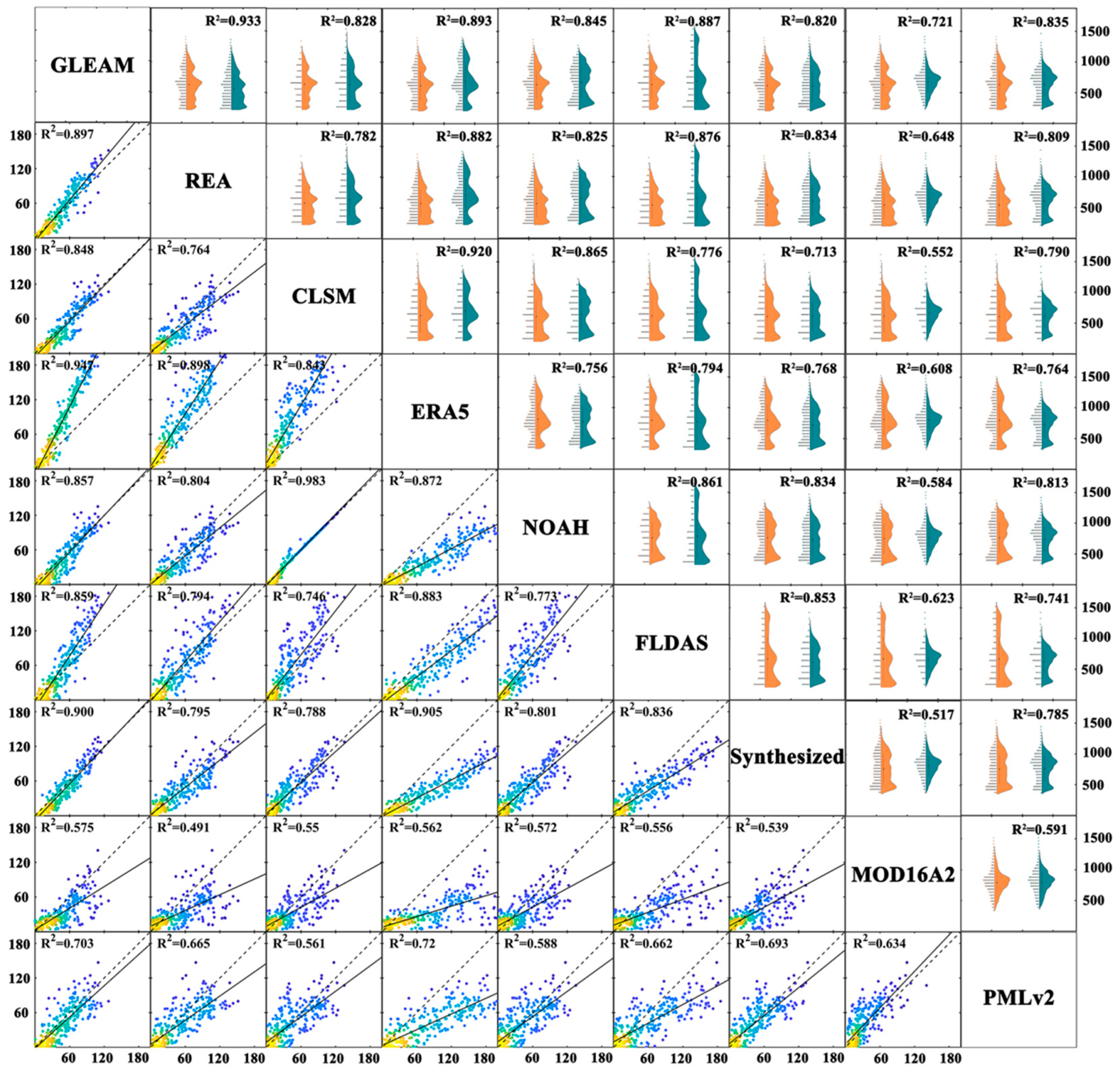
The spatial consistency of annual average ET estimated by nine grid products in China is illustrated in the upper triangle of Figure 2. Pairwise comparisons of ET products indicate significant spatial consistency among the products, except for MOD16A2. Overall, GLEAM and REA exhibit higher spatial consistency with other ET products, whereas MOD16A2 shows relatively lower spatial consistency. The highest spatial consistency is observed between GLEAM and REA (R2 = 0.933), followed by GLEAM and FLDAS (R2 = 0.887), while the lowest is between MOD16A2 and Syn (R2 = 0.517). The lower triangle of Figure 2 displays the temporal consistency of the monthly average ET among the products. In general, most R2 values exceed 0.8, except for comparisons between MOD16A2 and PMLv2. The highest temporal consistency is observed between CLSM and NOAH (R2 = 0.983).

3.1.2. Uncertainty Evaluation with TCH Method

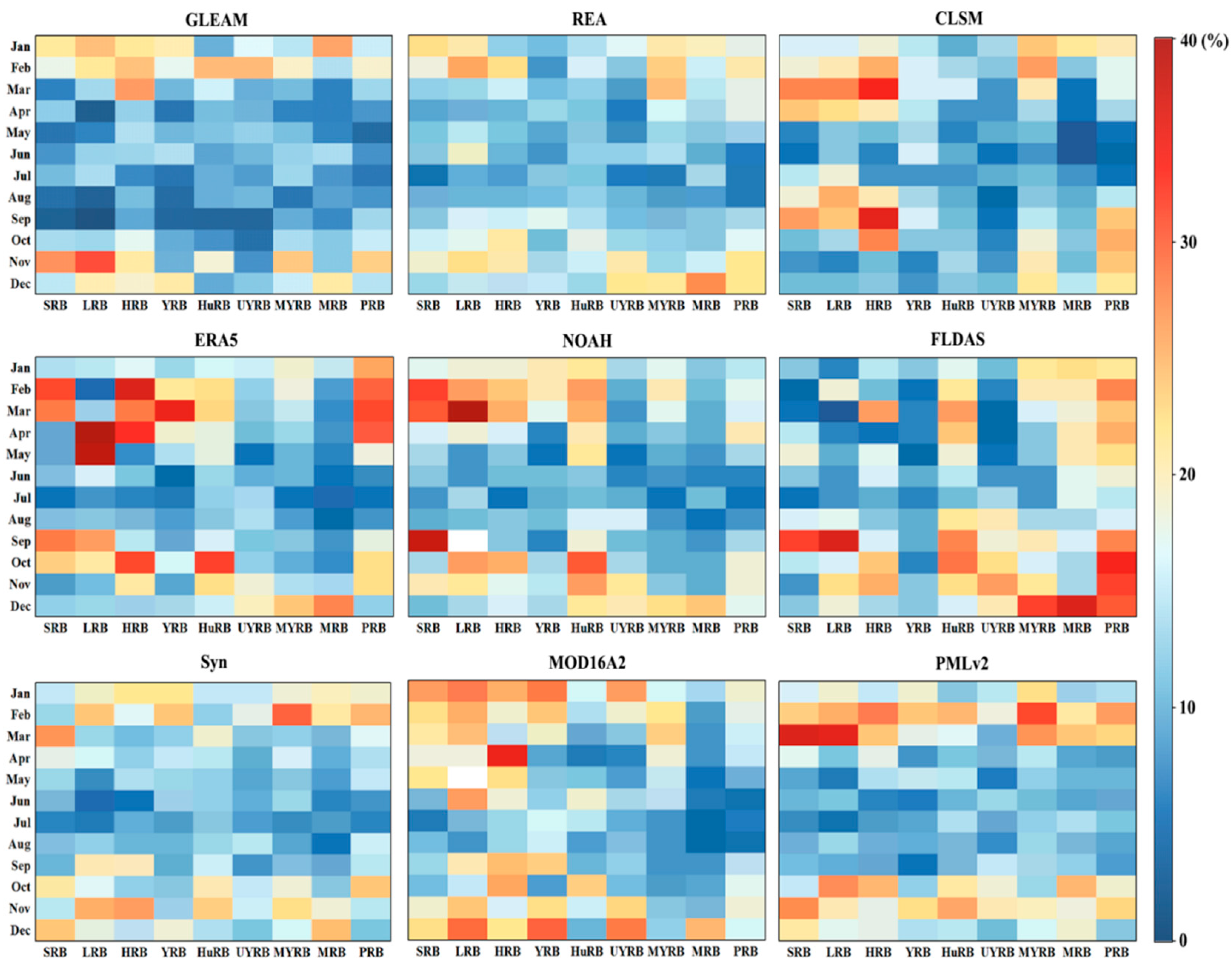
The uncertainties of the nine ET products across nine river basins were quantified using the TCH method (Figure 3). The results reveal significant variations in the uncertainties of different ET products across various basins. Among the nine ET products, GLEAM performed better in the HuRB (17.42 mm/month), MYRB (19.26 mm/month), and MRB (16.19 mm/month). REA exhibited the smallest RMSE in the SRB (12.41 mm/month) and HRB (12.25 mm/month), while Syn had the lowest uncertainty in the LRB (11.44 mm/month), YRB (9.62 mm/month), and UYRB (13.49 mm/month). The lowest uncertainty in the PRB basin was observed with PMLv2 (19.63 mm/month). Furthermore, from a basin-wide perspective, all ET products exhibited higher uncertainties in the HuRB, MYRB, MRB, and PRB, with values ranging between 16.19 mm/month and 39.81 mm/month. The YRB basin exhibited the lowest uncertainty, ranging from 9.61 mm/month to 18.09 mm/month. These variations illustrate the importance of considering local basin characteristics when evaluating model performance and uncertainty.
Relative uncertainty is the ratio of uncertainty to the monthly average ET, which allows for mitigating the impact of the ET magnitude itself. To further assess the uncertainty of ET, the monthly series of relative uncertainties for the nine ET products is displayed in Figure 4. Overall, most products perform better from April to September than from October to March. This performance trend may be due to the end of the snowmelt process and a more uniform distribution of rainfall during the warmer months, which typically results in more consistent surface moisture conditions, aiding in the more accurate simulation of the ET process. In contrast, snowmelt and uneven rainfall distribution during the colder months can complicate surface moisture conditions. Additionally, the effectiveness of simulating winter vegetation status, snow cover, and permafrost processes is reduced, increasing the uncertainty of ET estimates. Specifically, the GLEAM product shows poor performance in the SRB and LRB during winter, while PMLv2 exhibits slightly higher relative uncertainty during February and March, potentially due to ineffective simulation of sublimation from snow and ice and permafrost. MOD16A2 displays high relative uncertainties across all nine basins, particularly in the LRB and SRB. CLSM, ERA5, NOAH, and FLDAS show higher relative uncertainties during the summer months. Moreover, the two synthesized datasets, RE and Syn, exhibit relatively stable performance across different seasons regarding relative uncertainty.

3.2. Evaluation of ET Products at Basin Scale with Water Balance Method

Accuracy assessment of different ET products was performed based on water balance analysis at the basin scale from 2003 to 2014 (Table 5). Analysis across the nine basins revealed that GLEAM and Syn consistently outperformed other products across multiple statistical metrics. Specifically, GLEAM showed strong performance with R2 = 0.86, MAE = 16.83 mm/month, and RMSE = 22.94 mm/month, while Syn demonstrated comparable results with R2 = 0.89, MAE = 17.29 mm/month, and RMSE = 23.24 mm/month. However, in terms of systematic bias, the REA product performed best with a percent bias (Pbias) of −2.11%, indicating minimal overall overestimation or underestimation.
A clear performance hierarchy emerged among the products: CLSM and MOD16A2 exhibited the highest RMSE values, indicating relatively poor accuracy, followed by ERA5, NOAH, FLDAS, and PML with intermediate performance. In contrast, GLEAM, REA, and Syn consistently showed the lowest RMSE values (22.94, 24.41, and 23.24 mm/month, respectively), suggesting these products provide the most reliable ET estimates across diverse basin conditions.
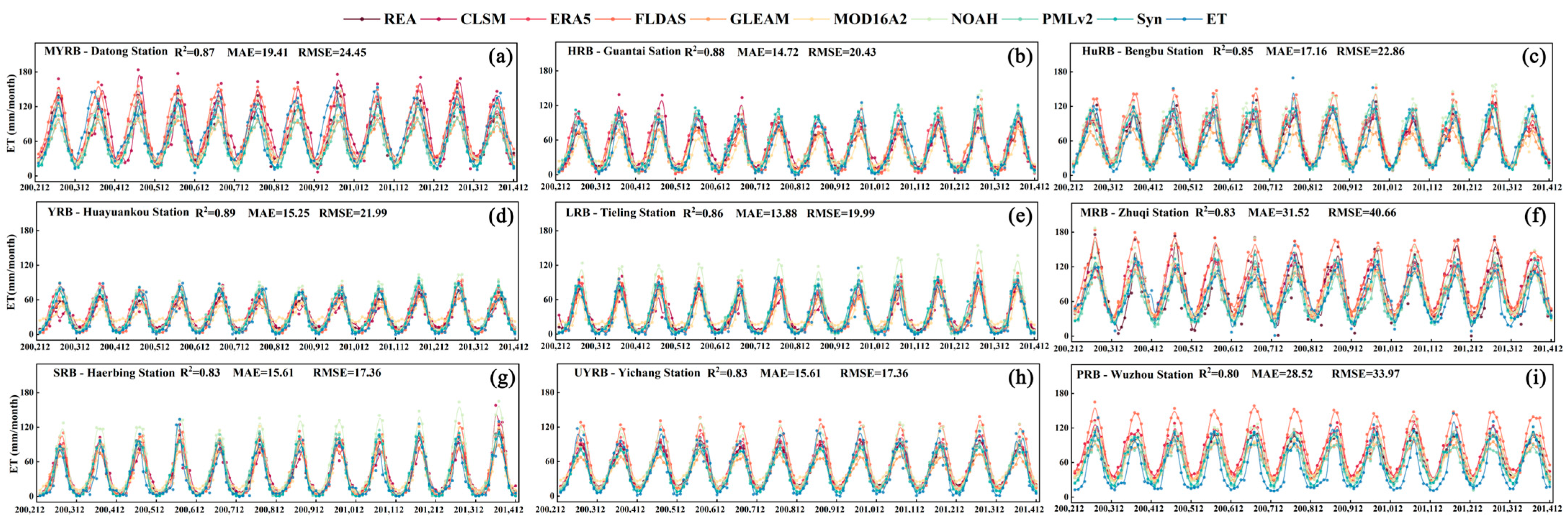
The monthly time series of ET for the nine basins are shown in Figure 5, and all 9 ET products do a good job of representing the changes in the seasonal cycle. In general, ET peaks in July and reaches its lowest value in January or December. However, a clear climate and region-specific performance pattern emerges from the statistical analysis (Appendix A Table A1), as no single product outperforms others across all basins. In terms of overall agreement with the WB-ET dataset, the UYRB basin exhibited the best performance, characterized by the highest correlation (R = 0.91) and the smallest MAE (RMSE) of 14.60 mm/month (18.97 mm/month). This was followed by the HRB, YRB, and LRB basins, which also showed strong statistical agreement. In contrast, the MRB and PRB basins demonstrated notably poorer performance, with larger errors (MAE and RMSE of 31.52 mm/month and 28.52 mm/month, respectively). This performance disparity suggests a potential influence of regional climatic conditions or land surface characteristics on the accuracy of ET products. The products generally performed better in the northern and interior basins (e.g., UYRB, HRB, YRB, LRB) compared to the southern and coastal basins (e.g., MRB, PRB), which may be associated with differences in humidity, precipitation regimes, or vegetation cover.

3.3. Accuracy of ET Products at Site Scale

3.3.1. Overall Conditions

The nine ET products are evaluated using flux tower observation data as a reference. Appendix A Figure A1 shows the correlation coefficients between ET products and ET estimates from different flux towers. The results indicate that the R for the nine ET products with observational data range from 0.43 to 0.96. Overall, MOD16A2 performed the poorest with an R range from 0.43 to 0.87, followed by PMLv2 and FLDAS. The products with the highest R were ERA5 and GLEAM. Notably, at the CN-Dan site, all ET products performed poorly, with R ranging from 0.65 to 0.79. Furthermore, the ubRMSE for ET products compared to observational data ranged from 2.18 mm/month to 35.42 mm/month. ERA5 exhibited the highest uncertainty, while GLEAM (ubRMSE = 11.57 mm/month) and Syn (ubRMSE = 11.70 mm/month) performed better regarding error metrics.
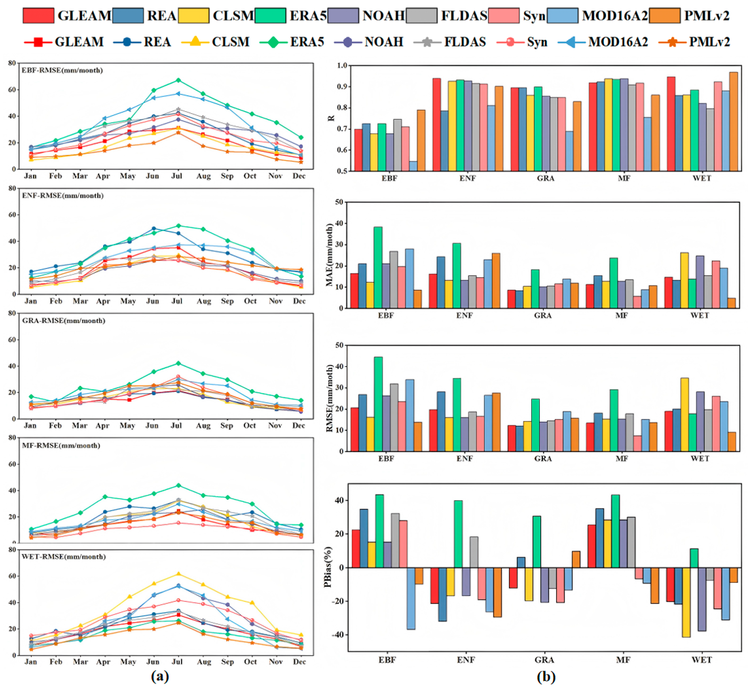
The ET estimation performance of different products under various cover types was assessed based on observations from 10 flux towers (Figure 6). Monthly time series ET data revealed that gridded ET products generally agreed with observational data, with both showing seasonal variations in ET without notable dependence on land cover type. Among the nine products, GLEAM, REA, and Syn produced ET estimates that are closer to observational data. Consequently, multiple indicators were further analyzed for variation across vegetation cover types (Figure 6b). In EBF, the correlation of ET products with observations is the poorest (R < 0.79), with MOD16A2 performing the worst (R = 0.55) and ERA5 having the largest root mean square error (RMSE = 44.59 mm/month); in ENF, GLEAM estimates perform best, while REA and MOD16A2 show weaker performance under this cover type; in GRA and MF, all products perform well; in WET, there is a relatively large variation in performance among products, with CLSM having the highest RMSE (34.69 mm/month) with observations, FLDAS having the lowest correlation, and GLEAM and PMLv2 performing best overall. Notably, ERA5 consistently shows the worst RMSE across all cover types, but its correlation with observational data is not weaker than that of other products. From a PBias perspective, ERA5 consistently presents a severe overestimation across all vegetation cover types, MOD16A2 displays an apparent underestimation across all types, while GLEAM and PMLv2 generally show better bias performance.

3.3.2. Performance of ET Products Under Different Temperature Conditions

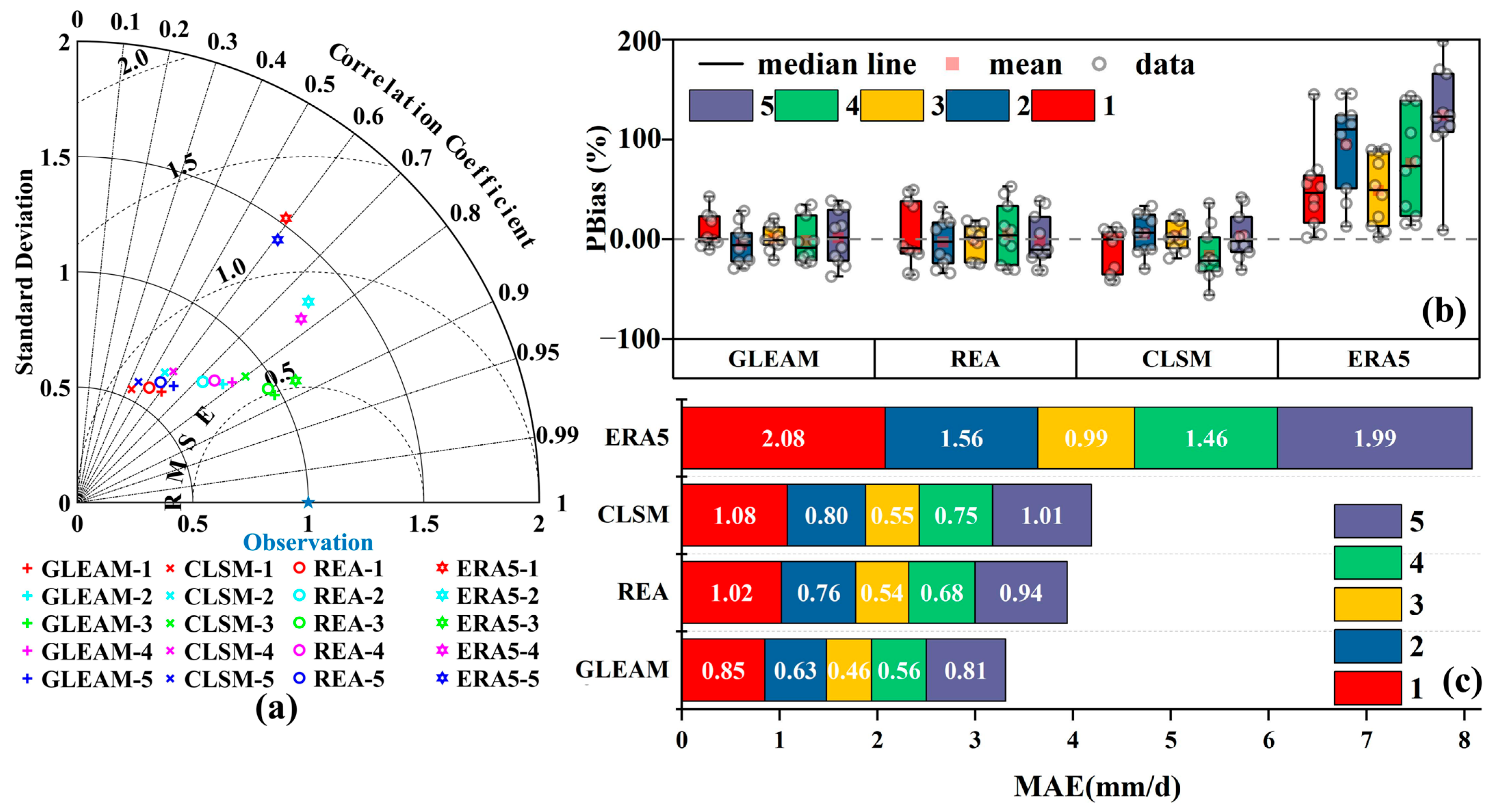
The estimation accuracy of daily-scale ET products is significantly affected by temperature conditions, especially under extreme high or low temperatures (Figure 7). Taylor diagrams illustrate that under various temperature conditions, GLEAM generally performs best, exhibiting the lowest performance of RMSE and MAE; REA is slightly inferior to GLEAM; CLSM shows the weakest correlation, with a root mean square error slightly higher than REA; although ERA5 has higher correlation, it displays the largest error. From the perspective of the degree of change in MAE (Figure 7), GLEAM shows the best performance, with MAE increasing by 85.4% (76.9%) under extreme high (low) temperatures. REA and CLSM are more affected than GLEAM, with increases of 87.8% (73.0%) and 94.8% (82.7%), respectively, while ERA5 is most affected by extreme temperatures, with MAE increases reaching 110.3% (101.4%). Percentage biases of the products under extreme temperature conditions show noticeable fluctuations. Specifically, GLEAM tends to significantly overestimate under high temperatures; both REA and CLSM show increased overestimations and underestimations under extreme high temperatures, while ERA5 consistently overestimates across all temperature conditions, with a particularly sharp increase in overestimation under extremely low temperatures. In summary, extreme temperatures significantly negatively impact the simulation accuracy of ET products. It is recommended to use GLEAM and REA for ET estimation under such conditions to achieve more reliable results.

3.3.3. Performance of ET Products Under Different VPD Conditions

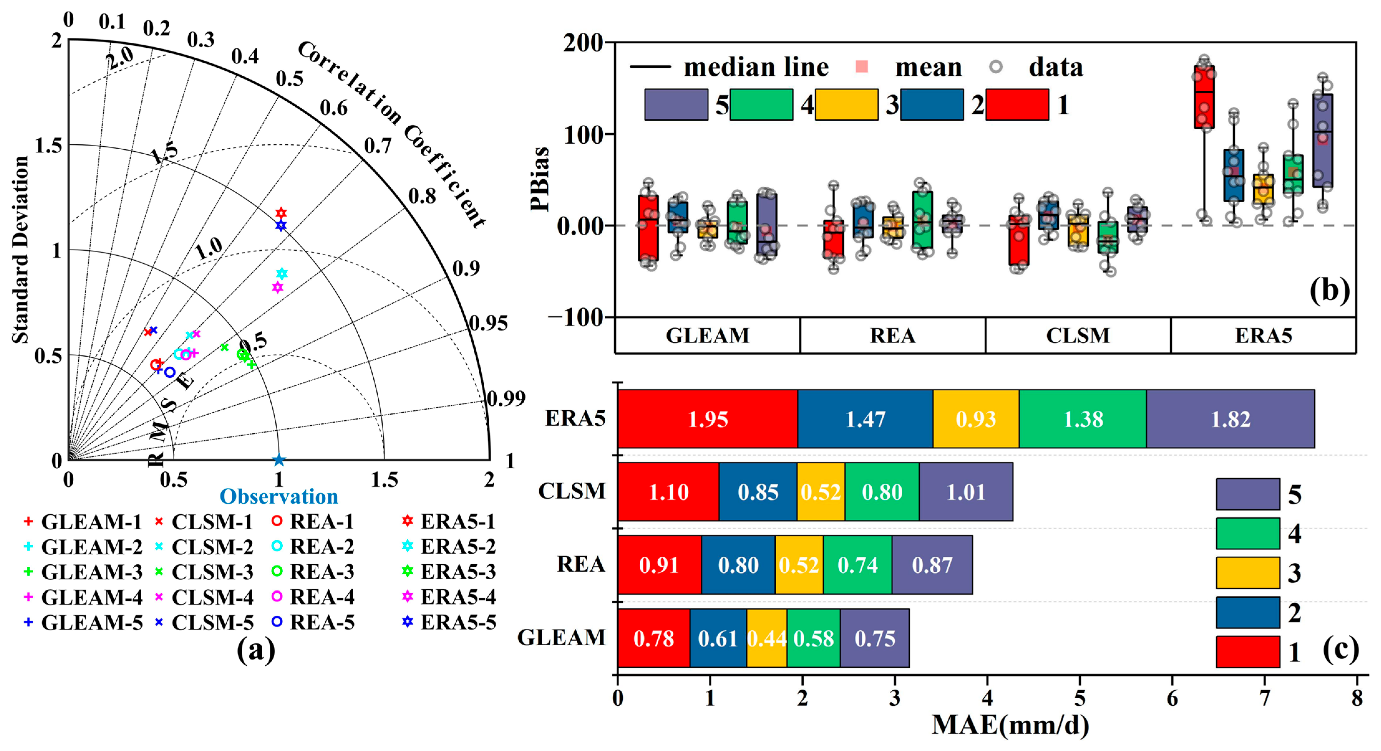
Figure 8 shows the estimation performance of four daily-scale ET products under five VPD conditions. The results indicate that the performance of all four products tends to decline from the middle (normal VPD) range towards extremes (extreme high VPD, high VPD, normal VPD, low VPD, and extreme low VPD). From Taylor diagrams (Figure 8), it is observed that under extreme high (low) VPD conditions, CLSM shows the poorest correlation (R < 0.6), while REA exhibits the best overall performance, with its correlation close to that of GLEAM and ERA5. Although ERA5 displays high correlation, it performs the worst in terms of error. Looking at the decline in MAE under different VPD conditions (Figure 8), REA is the least affected, with MAE increases of 74.4% (68.1%) under extreme high (low) VPD compared to normal VPD. GLEAM, CLSM, and ERA5 show MAE increases of 78.3% (70.1%), 112.4% (95.7%), and 108.5% (94.8%) under extreme high (low) VPD, respectively. The percentage bias of the products under different VPD conditions exhibits fluctuations, with a noticeable trend of increased overestimation and underestimation under extreme high (low) VPD conditions. Under these circumstances, the REA product is recommended for ET estimation.

3.3.4. Performance of ET Products Under Different Drought Conditions

The comparison of MAE for ET products under arid and non-arid conditions is displayed in Figure 9. The results indicate that the accuracy of ET products tends to decrease under arid conditions. Given that the monthly-scale resolution is coarser than the daily-scale, the detailed representation of site-specific characteristics by ET products is less distinct. Nevertheless, the majority of ET products exhibit weaker stability in arid conditions compared to non-arid conditions, with MAE increases by approximately 12–40%. There are noticeable differences in how various ET products respond to drought conditions. ERA5, FLDAS, and MOD16A2 show significant fluctuations in error when encountering arid conditions, leading to larger errors and a decline in stability. The remaining products experience varying degrees of decreased predictive stability under arid conditions, though the reduction is less pronounced.

3.3.5. Performance of ET Products Under Different Land Cover Types

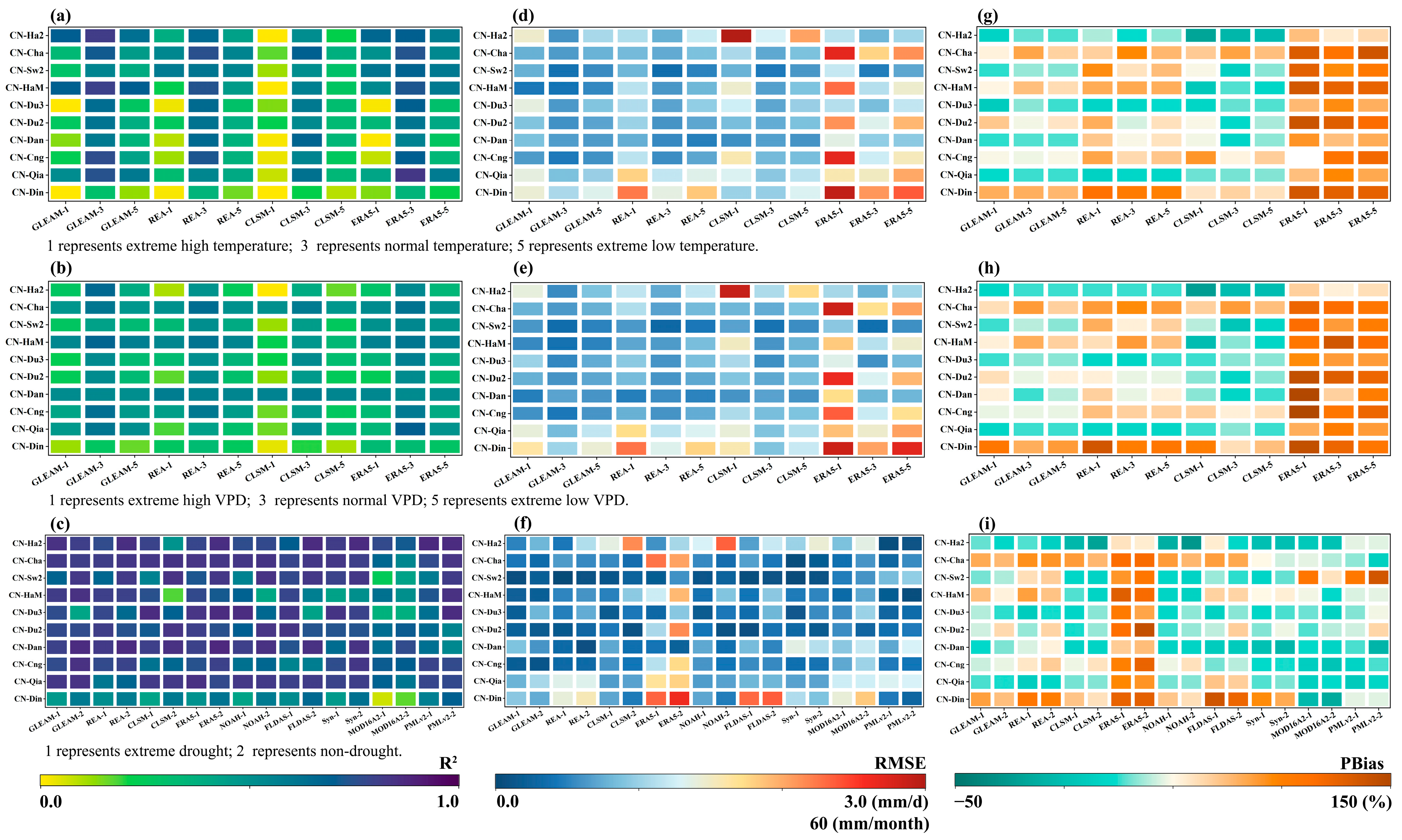
This paper compares ET products’ performance under extreme conditions at ten flux tower sites, with specific details in Figure 10. The results indicate that the estimation accuracy of all four daily-scale products and nine monthly-scale products deteriorates under extreme climatic conditions compared to normal climatic conditions. Specifically, the correlation performance of all ET products under extreme climatic conditions is worst at the EBF (CN-Din) site. For ENF (CN-Qia), the performance is relatively stable across the board; for WET (CN-Ha2) and MF (CN-Cha), GLEAM shows the best correlation performance under high temperature and VPD, respectively, while CLSM and ERA5 exhibit significant errors. The performance at GRA sites varies; for instance, GLEAM exhibits the highest estimation consistency under high temperatures at CN-Ham, whereas CLSM shows the lowest consistency, and CN-Du3 has a notably high RMSE. Finally, ERA5 consistently overestimates at all sites, while the other eight products exhibit a balanced number of sites with overestimations and underestimations. However, there is a notable overestimation in EBF and an underestimation in WET.

3.4. Improving the Accuracy of ET Estimation Under Extreme Climatic Conditions

The above study found that the estimation accuracy of most ET products is still not high, especially in extreme climatic conditions. In an attempt to improve the estimation of ET in such conditions, we utilized machine learning (ML) models to combine multiple ET products (Table 6) directly. The results show that when ET products are used as inputs to ML models, the estimation accuracy significantly improves, with random forest (RF) outperforming XGBoost (XGB) and Gaussian Process Regression (GPR) across all input combinations. Specifically, the estimation performance of the model improves as the number of input products increases, with the most significant improvement observed when the input combinations change from 1 to 2 products (R2 increases by up to 19.3%). Among the individual inputs, GLEAM delivers the best performance, but when all four daily-scale products are used together as inputs, the estimation accuracy of RF reaches its highest (R2 = 0.91, RMSE = 0.32 mm/d). This represents a 26.39% improvement in R2 and a 51.52% reduction in RMSE compared to GLEAM alone (R2 = 0.72, RMSE = 0.66 mm/d). Notably, the model with the input combination of 2A (GLEAM + ERA5) maintains high accuracy (RF_R2 = 0.89) with fewer input products, making it the most cost-effective combination. The improved performance in extreme climatic conditions, such as high/low temperatures, extreme VPD, and drought, indicates that machine learning models can effectively combine the strengths of different ET products, ensuring more reliable estimates under varying climatic scenarios.
In addition, under extreme climatic conditions, the RF model still exhibits significantly higher accuracy and stability than the traditional ET product, further verifying its adaptability under extreme climatic conditions. As shown in Table 5, the goodness-of-fit (R2) of the RF model increases from 0.25 to 0.72 at extreme temperatures, and the estimation error (RMSE) decreases to 0.61 mm/d. Similarly, the R2 of the RF model increases to 0.54–0.73 at extreme VPD, and the RMSE decreases to as low as 0.60 mm/d, which further confirms its adaptability under extreme climatic conditions. Accurate simulation of evapotranspiration behavior in the context of heat waves and atmospheric drought stress. It is worth noting that the RF model significantly outperforms the other two models, with R2 as high as 0.81 and RMSE as low as 11.26 mm/month. In general, this study innovatively uses a few ET products as machine learning inputs. It achieves excellent performance, frees the traditional method from relying on a large amount of meteorological data, and efficiently provides a new alternative method for estimating ET. Our study also demonstrates that the RF model not only performs well under normal climatic conditions but also has strong generalization ability and prediction accuracy in the face of extreme climatic conditions and thus has wide practical applications.
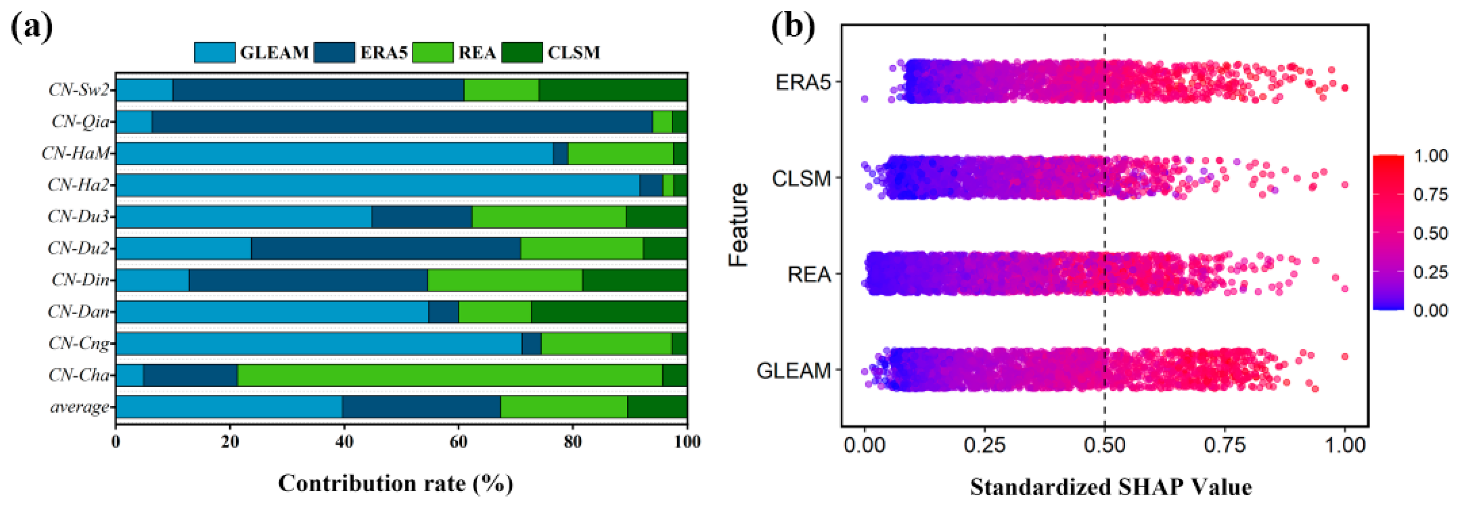
Finally, we discuss the contribution of the RF (best model) to each input product under input combination 4A (Figure 11). In general, GLEAM is the most important variable for RF in estimating ET at most sites, but results vary across sites. For example, under CN-Sw2, CN-Du2, and CN-Din, the percentage of ERA5 contribution is around 50%, while under CN-Qia, ERA5 contributes up to 87.6%. Overall, the contributions of both REA and CLSM are small, but the contribution of REA is relatively high under CN-Cha, while the contribution of CLSM is relatively high under CN-Sw2 and CN-Dan.
To further assess the contributions and dependencies of each input feature in the model, we quantified the SHAP summary plots of all standardized input features (Figure 11b). This plot demonstrates the distribution of the standardized SHAP values for each input feature along the horizontal axis, where the color of the dots indicates the magnitude of the feature values (with red representing high feature values and blue representing low feature values). From Figure 11b, we observe differences in the range of SHAP value distributions for each feature. However, most samples have contribution values concentrated within 0.5, indicating that each input variable has a balanced impact on model prediction. The color gradient further highlights the relationship between feature values and their contributions to the model, providing additional support for feature importance interpretation.
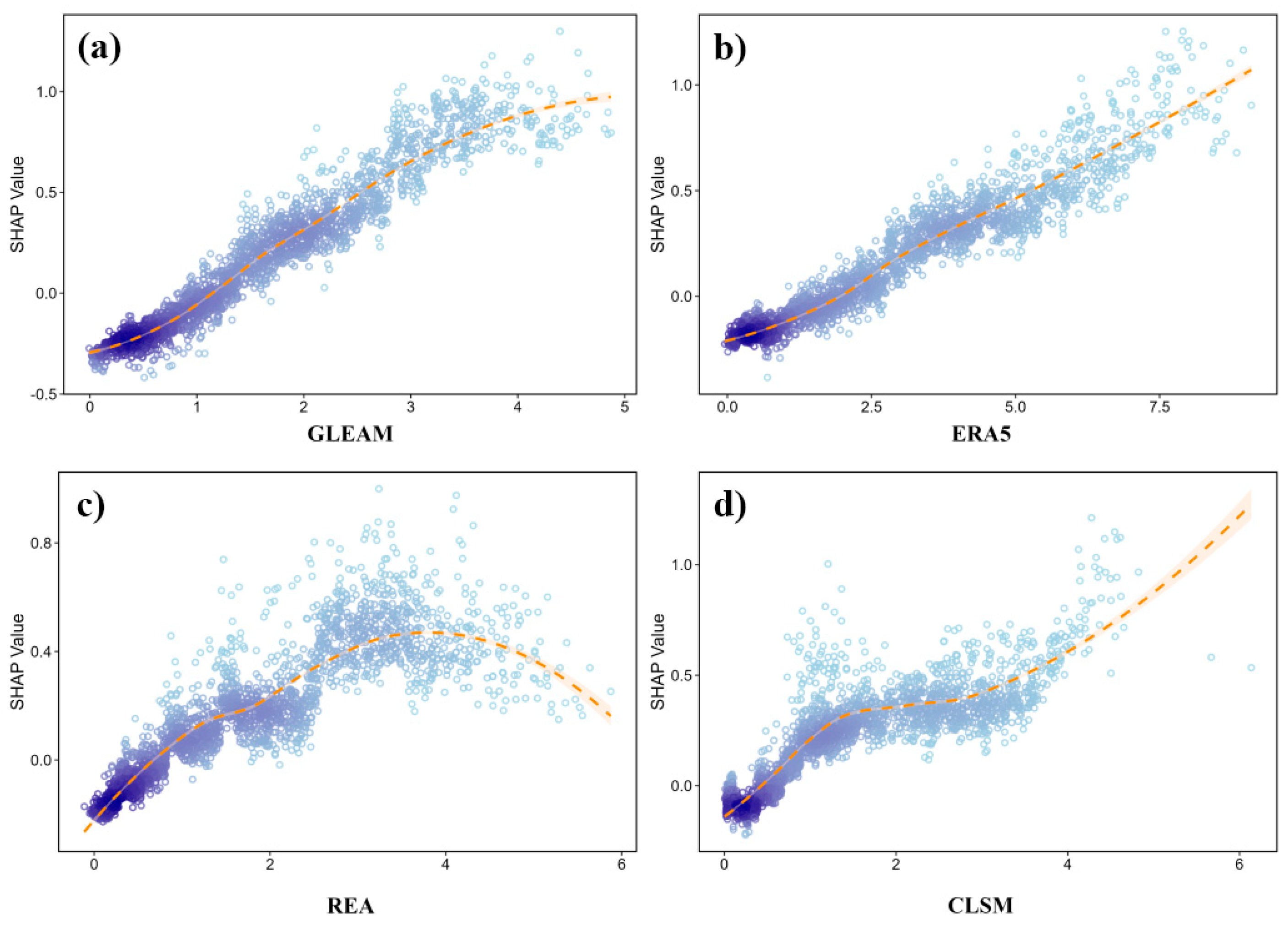
In Figure 12, we show the SHAP dependency plots for the four input variables (GLEAM, ERA5, REA, and CLSM). These plots reveal the nonlinear relationship between the effect of eigenvalue changes on model predictions. For instance, in Figure 12a, the SHAP value of GLEAM increases steadily with increasing eigenvalues, indicating a strong positive and stable relationship with model contribution. Similarly, Figure 12b shows that ERA5 also exhibits a positive influence, but its growth trend presents some nonlinear characteristics. In contrast, REA (Figure 12c) and CLSM (Figure 12d) exhibit more complex behavior. For both variables, the SHAP values rise rapidly at low eigenvalues and level off at higher values, suggesting that their marginal contributions to the model diminish at higher value ranges. The orange dashed line in each subfigure indicates the overall trend line, which helps to identify the main influence paths and change patterns of each variable.
In summary, the results systematically reveal the importance of the four ET products in the model output, their nonlinear contribution characteristics, and their varying impacts under different conditions. This further confirms their key roles in the ET estimation task and provides a theoretical basis for subsequent feature selection and model optimization.

4. Discussion

4.1. Uncertainty in Multi-Scale Evaluation Methods

This study evaluated nine ET products at the site and basin scales using flux tower observations and the water balance approach. Although these methods are widely adopted for multi-product assessments [28,34,65], we explicitly acknowledge that their intrinsic assumptions propagate non-negligible uncertainty and can partly explain product divergences reported here and elsewhere. EC covariance observations provide direct point-scale validation [25], yet the spatial representativeness of EC footprints (102–103 m) versus gridded products (104–105 m) introduces aggregation bias, particularly over heterogeneous mosaics of cropland–urban transitions [66]. In addition, EC energy-imbalance remains a longstanding issue [67]; we tested both “as-measured” and energy-closure-adjusted LE (by Bowen ratio and residual methods) and found that closure choices alter product rankings at several sites (notably EBF and WET), highlighting the need to report closure sensitivity alongside product skill.
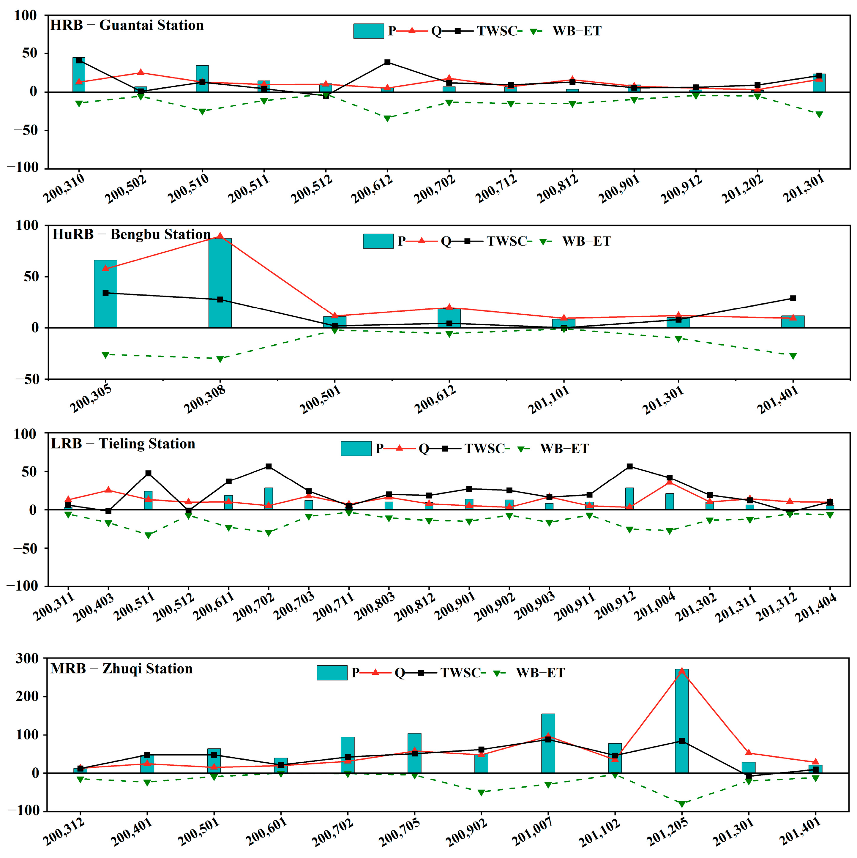
For basins, WB-ET as the residual of precipitation (P), runoff (Q), and GRACE-derived terrestrial water storage change (ΔTWSC) is affected by the accuracy of each term. Systematic under-catch in P (winter, orography), rating-curve uncertainties in Q, and GRACE leakage/scale effects (ΔTWSC) can jointly bias WB-ET; this is most consequential for small or hydrologically regulated basins (e.g., MRB) where GRACE footprint mismatch is significant. While some studies argue that ΔTWSC errors are negligible at the monthly scale [64,68], recent work emphasizes that neglecting ΔTWSC under climate anomalies or strong human regulation inflates WB-ET uncertainty (e.g., multi-year droughts, rapid reservoir storage swings). Our negative monthly WB-ET in LRB and MRB (Appendix A Figure A2) are consistent with these known limitations and should be interpreted as diagnostic flags rather than physical negatives. On the annual time scale, the multi-year average for 2003–2014 is shown in Appendix A Figure A3, with positive values observed in three of the nine basins, negative values in one basin, and close to zero in the remaining basins, which is very small and negligible compared to precipitation and runoff in the basins on the multi-year scale.

4.2. Uncertainty Analyses of Basins

The estimation of ET in river basins often overlooks the impact of human activities, such as irrigation and inter-basin water transfers, which significantly affect water movement within and outside sub-basins. Consequently, ET estimates in regions heavily influenced by these activities may exhibit higher uncertainty. HuRB, MYRB, MRB, and PRB show notably higher uncertainties among the nine river basins analyzed. In HuRB and MYRB, increased uncertainty is primarily attributed to the combined effects of reservoirs, urbanization, mining, agricultural changes, and canalization. For instance, in HuRB, where a large proportion of the land is dedicated to agriculture, ET is significantly influenced by agricultural activities. Agricultural water consumption accounted for 72.3% of the total water content in 2022, significantly impacting terrestrial water storage [69]. In the MRB, it arises from the high number of reservoirs and widespread lakes, which alter runoff patterns, while in the MRB, the basin’s small size (550,000 km2) falls below the typical resolution of GRACE satellites (100,000 km2), amplifying noise in water storage calculations and increasing ET uncertainty. In addition, variations in lake levels further disrupt runoff estimations [70].
The PRB, spanning tropical and subtropical zones, faces complex meteorological conditions, including monsoonal climates and typhoons, which introduce variability in ET estimates. The diversity of land cover types in PRB also contributes to the increased uncertainty, as differences in surface cover affect water cycling, complicating the estimation of ET in the region [71]. These findings are consistent with recent studies, which emphasize the need to incorporate human water management modules, such as irrigation signals, to reduce bias in ET retrievals, as ET product performance declines under high-intensity irrigation and reservoir operations. For instance, Liu et al. [72] found that incorporating irrigation signals extracted from Landsat 8 to calibrate the SWAT model reduced ET underestimation from 24.4% to 6.9%, aligning closely with our results. Castle et al. [73] found that human water management, such as irrigation, contributes up to 38% of the ET in the Colorado River Basin. Based on these observations, we recommend adopting basin-specific product portfolios, particularly recommending Syn/REA for areas with moderate regulation, and GLEAM/PMLv2 for cropland-dominated basins after bias-correction against irrigation schedules.

4.3. Advantages of ET Product-Based Machine Learning Modeling and Its Interpretability

The results of this study further validate the effectiveness and potential of ET products as machine learning input variables in ET estimation. Compared to the traditional practice of using multiple meteorological factors, using ET products as the primary input significantly simplifies the model’s input dimensions while improving its practicality and adaptability without sacrificing accuracy [74]. This simplification strategy is particularly advantageous for regions with scarce or low-quality meteorological data, enabling more stable and reliable ET estimation at a lower data cost [23].
From the interpretability perspective, ET products as machine learning input variables not only reduce the data dimensionality but also have a more physically meaningful representation. ET products are results of integrated simulation or remote sensing inversion based on the principle of energy balance, vegetation response, moisture dynamics, and other processes [64], which comprehensively reflect the effects of key meteorological and surface factors [75]. Consequently, ET products can directly represent actual surface evapotranspiration in a more “process-oriented” manner than basic meteorological variables like temperature, humidity, and wind speed [50,76]. This integration reduces the burden of model fitting in the presence of complex nonlinear relationships among input variables, improving the stability of the learning process and ensuring result consistency [77]. Moreover, since ET products are often validated and calibrated over long periods, their spatial and temporal distribution characteristics align well with surface vegetation, soil moisture, and climatic conditions, making the behavior of their inputs in the model clearly process-directed [78], and making them more physically interpretable and enhancing model transparency [79]. Using ET products as input variables also helps avoid uncertainties caused by missing meteorological data or sensor errors, improving the robustness and generalizability of the model [80]. Therefore, it is not detached from the physical meaning of ET, but can be used as an “integrated variable” to help the model capture the spatial and temporal changes of ET more directly, and has a better basis for physical interpretation and process representation.
Finally, the random forest model used in this study demonstrates good adaptability, as its integrated learning method reduces overfitting through averaging multiple decision trees and effectively models nonlinear relationships between input variables [81]. Its inherent variable importance mechanism also aids in understanding the contribution of each input variable to ET estimates, enhancing the interpretability and transparency of the model.

4.4. Uncertainty of ET Products Under Extreme Climatic Conditions

Research has demonstrated that ET products exhibit significant uncertainty under extreme climatic conditions, corroborating the findings of Yu et al. [27]. The underlying causes are multifaceted and require a nuanced analysis. Key contributors to this uncertainty include the increased complexity of land surface characteristics under extreme conditions. These factors-such as heterogeneous soil moisture, variability in vegetation cover, and diverse soil types-complicate the evapotranspiration process, making accurate simulation and forecasting of ET difficult [82]. Furthermore, the uncertainty inherent in model parameters also plays a pivotal role. ET models depend on various parameters, such as vegetation characteristics and soil water conductivity [83]. Under extreme conditions, the accuracy of these parameters may be compromised, thus affecting the reliability of ET estimates. For instance, soil water conductivity might alter during drought conditions, and accurately capturing its effect on ET could prove challenging. Moreover, the paucity of observational data restricts precise predictions of ET under extreme conditions [84]. The acquisition of observational data becomes increasingly challenging under extreme climatic conditions, particularly when remote sensing data acquisition is hindered by cloud cover. This limitation diminishes the models’ capacity to accurately characterize surface features, subsequently affecting the estimation of ET [42].

4.5. Contributions and Limitations

Currently, there is a lack of systematic uncertainty analysis of evapotranspiration (ET) products at the watershed scale and under different extreme climatic conditions [18,34]. While previous studies have quantified ET uncertainty at both watershed and grid scales and explored the impact of drought on ET, a comprehensive assessment under extreme climatic conditions is still lacking [11]. In the multi-scale (grid, watershed, and site) ET product evaluations in China, most existing work is limited to normal climatic conditions and does not cover the impact of different climatic scenarios [35,36]. Similarly, ET validation and estimation studies at the watershed scale based on multi-source remote sensing data often assume normal meteorological conditions and have not fully considered the impact of climate variability on ET [37,38]. Although some studies have pointed out that ET products are affected by extreme climatic conditions, a comprehensive and systematic assessment of the specific response mechanisms at different watershed and grid scales in China is still lacking [27,33]. In contrast, this study systematically evaluates the performance of ET products under extreme high temperatures, low temperatures, vapor pressure deficit, and drought conditions across multiple scales (grid, watershed, and site), filling the gap in current research. By refining the classification of extreme climate types and conducting multi-dimensional analysis, this study reveals the differences and limitations of various ET products in extreme environments, clarifies the underlying mechanisms, and examines the impact of human activities on watershed-scale results. Additionally, a cost-effective machine learning fusion method is proposed, providing a scientific basis for climate change adaptation, ET product selection, and improvement, thus enhancing the practical value of the research.
Although this study provides new perspectives and methods, there are still some limitations and room for future improvement. First, the impact of human activities has not been fully incorporated into the model analysis, particularly factors such as agricultural irrigation, reservoir regulation, and inter-basin water transfers. These human activities significantly influence watershed hydrological cycles and ET, so future research should consider the impact of human activities on ET estimation uncertainty more comprehensively and incorporate socio-economic factors. Second, the GRACE data used in this study have certain limitations, especially in ET estimation for small watersheds and high-resolution areas. The spatial resolution of GRACE restricts its application in fine-scale analysis. Future research can improve accuracy by integrating high-resolution satellite data (e.g., soil moisture and vegetation indices) and remote sensing data and supplementing with more ground-based observational data for validation and enhancement. Moreover, although the TCH method was used in this study to quantify the uncertainty of ET products, this method has certain assumptions and may not fully reflect the complex uncertainties caused by climate and human factors in some watersheds. Future studies could combine physical models and machine learning methods to achieve more accurate and comprehensive ET predictions. Under extreme climatic conditions, the acquisition and quality of remote sensing data remain limiting factors. Cloud cover, satellite orbits, and instrument failures may affect data availability and quality. With advancements in remote sensing technology and data processing techniques, more reliance on multi-source data fusion could solve these problems and improve model robustness and generalization ability. Additionally, the lack of comprehensive observational data, particularly in some extreme climate regions, still limits the accuracy and widespread application of models. Future studies can focus on overcoming these data gaps, such as by fostering cross-regional cooperation, enhancing the observational station network, or filling gaps through simulation and extrapolation. Overall, although the methods and data used in this study provide valuable support for ET estimation, with the ongoing impacts of climate change and human activities, continuous optimization of models and integration of more remote sensing and ground-based observational data are essential to improving the reliability and accuracy of ET estimates in different regions and under extreme conditions.

5. Conclusions

Accurately calculating evapotranspiration (ET) is crucial in the context of global warming and intensified climate change, especially for applications in water resource management and sustainable agriculture. This study systematically evaluates the consistency and uncertainty of nine gridded ET products (GLEAM, REA, CLSM, ERA5, NOAH, FLDAS, Syn, MOD16A2, and PMLv2) across China, particularly under varying climatic conditions. Our findings address the issue that current ET products often fail to provide reliable estimations under extreme climatic conditions, which are critical for effective water resource management. The main conclusions are as follows:
(1)
At the grid scale, spatial and temporal consistency of the nine ET products was assessed, revealing high consistency across products. GLEAM exhibited the highest consistency, while MOD16A2 showed the lowest. The uncertainty analyses using the TCH method revealed significant variation in product performance across basins. GLEAM, REA, and Syn performed with low uncertainty in several basins, highlighting their robustness for large-scale applications;
(2)
At the basin scale, the accuracy of nine ET products was evaluated across nine major river basins using the water balance method. Results indicate strong agreement with water-balance-based ET, with GLEAM showing the smallest error (MAE = 16.83 mm/month, RMSE = 22.94 mm/month), REA the smallest bias (PBias = −2.11%), and Syn the highest correlation (R2 = 0.89);
(3)
At the site scale, performance was analyzed using flux tower observations under different climatic conditions. All products showed declining accuracy from moderate (normal temperature/VPD) to extreme conditions (extreme high/low temperature and VPD). Under extreme high temperature/VPD and extreme low temperature/VPD, MAE increased by 110.32% (112.45%) and 101.4% (95.71%), respectively. In contrast, drought led to less severe degradation, with MAE rising by 12–40%. Among the nine products, GLEAM and REA exhibited relatively small performance losses, while ERA5 performed worst under extreme conditions;
(4)
In machine learning applications, using a few high-quality daily ET products as inputs substantially improved accuracy, especially under extreme climates, and avoided reliance on numerous traditional meteorological factors. The random forest (RF) model performed best, achieving R2 up to 0.91 (RMSE = 0.32 mm/d) under overall conditions, far surpassing single products, while maintaining strong generalization under extreme temperature (R2 up to 0.72), extreme VPD (R2 up to 0.73), and drought (R2 up to 0.81). GLEAM was consistently the most important input for RF at most sites.
In summary, our findings not only quantify the uncertainties but also provide practical guidance for selecting and improving ET products. For practical applications in water resource management, we recommend prioritizing the use of GLEAM and REA products for large-scale monitoring and modeling in China due to their overall lower uncertainty and higher robustness. Secondly, under extreme temperature/VPD conditions, the use of single products (especially ERA5 and MOD16A2) should be cautious; instead, blended products or the machine learning-corrected values generated in this study could be considered for more reliable estimates. Future research should focus on improving ET algorithms to better represent physiological responses under extreme conditions and expanding machine learning methods to integrate more diverse data sources, promoting applications worldwide. This study provides important guiding principles for precision irrigation, climate adaptation, and sustainable agriculture.

Supplementary Materials

The following supporting information can be downloaded at https://www.mdpi.com/article/10.3390/agriculture15181945/s1.

Author Contributions

Conceptualization, L.Q. and L.W.; methodology, L.Q.; software, L.Q., N.D., and X.B.; validation, L.Q., T.D. and X.B.; formal analysis, L.Q. and X.Y.; investigation, X.L.; resources, Q.Y. and Z.Z.; data curation, L.Q.; writing—original draft preparation, L.Q.; visualization, J.C.; supervision, L.Q. and Z.Z.; project administration, Q.Y. and Z.Z.; funding acquisition, Z.Z. All authors have read and agreed to the published version of the manuscript.

Funding

This research was funded by the National Key Research and Development Program of China (2022YFD1900404) and the National Natural Science Foundation of China (51979232, 52179044).

Institutional Review Board Statement

Not applicable.

Data Availability Statement

The data presented in this study are available on request from the corresponding author.

Acknowledgments

The data used in this study are public, and the access links to the original dataset are located in the corresponding sections of Materials and Methods. We thank all the individuals and organizations that provided public data for this study.

Conflicts of Interest

The authors declare no conflicts of interest.

Appendix A

Figure A1. Comparison of R (left) and ubRMSE (right) of ET products at different flux towers.
Agriculture 15 01945 g0a1
Figure A2. Months with negative ET counterparts for the period 2003–2014. P is rainfall, Q is runoff, and WB-ET is the monthly-scale water balance calculated ET, all in (mm).
Agriculture 15 01945 g0a2
Figure A3. Monthly ∆TWSC and annual ∆TWSC mean derived from GRACE satellite for nine basins for the period 2002-2013.
Agriculture 15 01945 g0a3
Table A1. Comparison of the performance of water balance-based calculated ET and nine models estimated ET in different basins.
ET ProductsBasinsSRBLRBHRBYRBHuRBUYRBMYRBMRBPRB
GLEAMR0.800.870.870.930.850.910.900.830.81
MAE12.2513.7915.1716.4820.2816.0121.0115.7520.73
RMSE18.6921.0820.8322.4526.5720.125.2824.2427.22
REAR0.850.890.920.920.860.920.840.790.78
MAE14.212.7613.3815.4613.8213.9717.6633.4930.75
RMSE21.2918.4218.9423.0619.0717.4223.0342.5435.93
CLSMR0.750.720.850.780.860.910.750.800.82
MAE19.2617.4716.6819.4714.1113.2225.4431.5528.14
RMSE27.4525.7921.627.9618.81731.1341.1132.54
ERA5R0.820.890.860.900.830.910.880.850.79
MAE16.2211.9315.5912.7219.0914.3915.2234.535.56
RMSE24.117.4823.7919.1925.5518.8319.3645.0239.44
NOAHR0.850.890.900.920.840.900.870.850.81
MAE21.2217.0913.511.7124.3415.3514.9329.8128.67
RMSE3124.1718.4316.3729.7320.1919.8638.6733.41
FLDASR0.830.880.870.930.840.900.880.840.83
MAE13.511.1412.4411.1920.8315.1218.7922.633.25
RMSE21.8317.3418.817.3827.3120.6623.3228.7943.73
SynR0.860.900.910.880.890.920.890.860.83
MAE13.6611.4312.2413.5113.8612.2418.5936.7123.42
RMSE20.9516.0916.8621.0718.8217.223.4845.3329.34
MOD16A2R0.840.830.870.860.830.900.880.850.79
MAE15.4817.7921.0523.7714.6518.6819.5434.5627.98
RMSE22.1123.3427.0630.5121.4722.1125.1945.0733.11
PMLv2R0.850.890.900.880.870.910.900.830.78
MAE14.7211.5612.4212.9713.4712.423.544.723.22
RMSE22.0216.2617.5319.8718.417.229.4355.1531.03

References

  1. Mathew, F.M.; Wood, E.F. Scale Influences on the Remote Estimation of Evapotranspiration Using Multiple Satellite Sensors. Remote Sens. Environ. 2006, 105, 271–285. [Google Scholar] [CrossRef]
  2. Trenberth, K.E.; Smith, L.; Qian, T.T.; Dai, A.; Fasullo, J. Estimates of the Global Water Budget and Its Annual Cycle Using Observational and Model Data. J. Hydrometeorol. 2007, 8, 758–769. [Google Scholar] [CrossRef]
  3. Oki, T.; Kanae, S. Global Hydrological Cycles and World Water Resources. Science 2006, 313, 1068–1072. [Google Scholar] [CrossRef]
  4. Piao, S.L.; Zhang, X.P.; Chen, A.P.; Liu, Q.; Lian, X.; Wang, X.H.; Peng, S.S.; Wu, X.C. The Impacts of Climate Extremes on the Terrestrial Carbon Cycle: A Review. Sci. China Earth Sci. 2019, 62, 1551–1563. [Google Scholar] [CrossRef]
  5. Sorokin, Y.; Zelikova, T.J.; Blumenthal, D.; Williams, D.G.; Pendall, E. Seasonally Contrasting Responses of Evapotranspiration to Warming and Elevated CO2 in a Semiarid Grassland. Ecohydrology 2017, 10, e1880. [Google Scholar] [CrossRef]
  6. Vicente-Serrano, S.M.; Miralles, D.G.; Domínguez-Castro, F.; Azorin-Molina, C.; El Kenawy, A.; McVicar, T.R.; Tomás-Burguera, M.; Beguería, S.; Maneta, M.; Peña-Gallardo, M. Global Assessment of the Standardized Evapotranspiration Deficit Index (SEDI) for Drought Analysis and Monitoring. J. Clim. 2018, 31, 5371–5393. [Google Scholar] [CrossRef]
  7. Wang, K.C.; Dickinson, R.E. A Review of Global Terrestrial Evapotranspiration: Observation, Modeling, Climatology, and Climatic Variability. Rev. Geophys. 2012, 50, RG2005. [Google Scholar] [CrossRef]
  8. dos Santos, R.A.; Mantovani, E.C.; Bufon, V.B.; Fernandes-Filho, E.I. Improving Actual Evapotranspiration Estimates Through an Integrated Remote Sensing and Cutting-Edge Machine Learning Approach. Comput. Electron. Agric. 2024, 225, 109258. [Google Scholar] [CrossRef]
  9. Liu, Y.J.; Wang, W.; Zhao, T.Q.; Huo, Z.Y. Performance Evaluation and Spatiotemporal Dynamics of Nine Reanalysis and Remote Sensing Evapotranspiration Products in China. Remote Sens. 2025, 17, 1881. [Google Scholar] [CrossRef]
  10. Long, D.; Longuevergne, L.; Scanlon, B.R. Uncertainty in Evapotranspiration from Land Surface Modeling, Remote Sensing, and GRACE Satellites. Water Resour. Res. 2014, 50, 1131–1151. [Google Scholar] [CrossRef]
  11. Xu, T.; Guo, Z.; Xia, Y.; Ferreira, V.G.; Liu, S.; Wang, K.; Yao, Y.; Zhang, X.; Zhao, C. Evaluation of Twelve Evapotranspiration Products from Machine Learning, Remote Sensing and Land Surface Models over Conterminous United States. J. Hydrol. 2019, 578, 124105. [Google Scholar] [CrossRef]
  12. Jung, M.; Reichstein, M.; Ciais, P.; Seneviratne, S.I.; Sheffield, J.; Goulden, M.L.; Bonan, G.; Cescatti, A.; Chen, J.Q.; de Jeu, R.; et al. Recent Decline in the Global Land Evapotranspiration Trend Due to Limited Moisture Supply. Nature 2010, 467, 951–954. [Google Scholar] [CrossRef]
  13. Senay, G.B.; Bohms, S.; Singh, R.K.; Gowda, P.H.; Velpuri, N.M.; Alemu, H.; Verdin, J.P. Operational Evapotranspiration Mapping Using Remote Sensing and Weather Datasets: A New Parameterization for the SSEB Approach. J. Am. Water Resour. Assoc. 2013, 49, 577–591. [Google Scholar] [CrossRef]
  14. Xia, Y.L.; Hobbins, M.T.; Mu, Q.Z.; Ek, M.B. Evaluation of NLDAS-2 Evapotranspiration Against Tower Flux Site Observations. Hydrol. Process. 2015, 29, 1757–1771. [Google Scholar] [CrossRef]
  15. Mueller, B.; Seneviratne, S.I.; Jimenez, C.; Corti, T.; Hirschi, M.; Balsamo, G.; Ciais, P.; Dirmeyer, P.; Fisher, J.B.; Guo, Z.; et al. Evaluation of Global Observations-Based Evapotranspiration Datasets and IPCC AR4 Simulations. Geophys. Res. Lett. 2011, 38, L06406. [Google Scholar] [CrossRef]
  16. Miralles, D.G.; Jiménez, C.; Jung, M.; Michel, D.; Ershadi, A.; McCabe, M.F.; Hirschi, M.; Martens, B.; Dolman, A.J.; Fisher, J.B.; et al. The WACMOS-ET Project—Part 2: Evaluation of Global Terrestrial Evaporation Data Sets. Hydrol. Earth Syst. Sci. 2016, 20, 823–842. [Google Scholar] [CrossRef]
  17. Khan, M.S.; Liaqat, U.W.; Baik, J.; Choi, M. Stand-Alone Uncertainty Characterization of GLEAM, GLDAS and MOD16 Evapotranspiration Products Using an Extended Triple Collocation Approach. Agric. For. Meteorol. 2018, 252, 256–268. [Google Scholar] [CrossRef]
  18. Li, Q.; Liu, X.; Zhong, Y.; Wang, M.; Zhu, S. Estimation of Terrestrial Water Storage Changes at Small Basin Scales Based on Multi-Source Data. Remote Sens. 2021, 13, 3304. [Google Scholar] [CrossRef]
  19. Zhang, X.; Li, J.B.; Wang, Z.F.; Dong, Q.J. Global Hydroclimatic Drivers of Terrestrial Water Storage Changes in Different Climates. Catena 2022, 219, 106598. [Google Scholar] [CrossRef]
  20. Fang, P.; Wang, T.; Yang, D.; Tang, L.; Yang, Y. Substantial Increases in Compound Climate Extremes and Associated Socio-Economic Exposure across China under Future Climate Change. npj Clim. Atmos. Sci. 2025, 8, 17. [Google Scholar] [CrossRef]
  21. Robinson, A.; Lehmann, J.; Barriopedro, D.; Rahmstorf, S.; Coumou, D. Increasing Heat and Rainfall Extremes Now Far Outside the Historical Climate. npj Clim. Atmos. Sci. 2021, 4, 45. [Google Scholar] [CrossRef]
  22. Tang, Y.; Luo, M.; Wu, S.; Li, X. Increasing Synchrony of Extreme Heat and Precipitation Events Under Climate Warming. Geophys. Res. Lett. 2025, 52, e2024GL113021. [Google Scholar] [CrossRef]
  23. Coumou, D.; Rahmstorf, S. A Decade of Weather Extremes. Nat. Clim. Change 2012, 2, 491–496. [Google Scholar] [CrossRef]
  24. Zhu, B.Y.; Sun, B.; Wang, H.J. Increased interannual variability in the dipole mode of extreme high-temperature events over East China during summer after the early 1990s and associated mechanisms. J. Clim. 2022, 35, 1347–1364. [Google Scholar] [CrossRef]
  25. Pérez, J.; Correa-Araneda, F.; López-Rojo, N.; Basaguren, A.; Boyero, L. Extreme temperature events alter stream ecosystem functioning. Ecol. Indic. 2021, 121, 106984. [Google Scholar] [CrossRef]
  26. Wang, P.; Yamanaka, T.; Li, X.; Wei, Z. Partitioning evapotranspiration in a temperate grassland ecosystem: Numerical modeling with isotopic tracers. Agric. For. Meteorol. 2015, 208, 16–31. [Google Scholar] [CrossRef]
  27. Yu, X.J.; Qian, L.; Wang, W.E.; Hu, X.T.; Dong, J.H.; Pi, Y.Y.; Fan, K. Comprehensive evaluation of terrestrial evapotranspiration from different models under extreme condition over conterminous United States. Agric. Water Manag. 2023, 289, 108555. [Google Scholar] [CrossRef]
  28. Ochege, F.U.; Shi, H.; Li, C.; Ma, X.; Igboeli, E.E.; Luo, G. Assessing Satellite, Land Surface Model and Reanalysis Evapotranspiration Products in the Absence of In-Situ in Central Asia. Remote Sens. 2021, 13, 5148. [Google Scholar] [CrossRef]
  29. Panahi, M.D.; Tabas, S.S.; Kalantari, Z.; Ferreira, C.S.S.; Zahabiyoun, B. Spatio-Temporal Assessment of Global Gridded Evapotranspiration Datasets across Iran. Remote Sens. 2021, 13, 1816. [Google Scholar] [CrossRef]
  30. Wang, Z.; Cui, Z.; He, T.; Tang, Q.; Xiao, P.; Zhang, P.; Wang, L. Attributing the Evapotranspiration Trend in the Upper and Middle Reaches of Yellow River Basin Using Global Evapotranspiration Products. Remote Sens. 2022, 14, 175. [Google Scholar] [CrossRef]
  31. Herman, M.R.; Nejadhashemi, A.P.; Hernandez-Suarez, J.S.; Sadeghi, A.M. Analyzing the Variability of Remote Sensing and Hydrologic Model Evapotranspiration Products in a Watershed in Michigan. J. Am. Water Resour. Assoc. 2020, 56, 738–755. [Google Scholar] [CrossRef]
  32. Baik, J.; Liaqat, U.W.; Choi, M. Assessment of satellite- and reanalysis-based evapotranspiration products with two blending approaches over the complex landscapes and climates of Australia. Agric. For. Meteorol. 2018, 263, 388–398. [Google Scholar] [CrossRef]
  33. Qian, L.; Zhang, Z.T.; Wu, L.F.; Fan, S.S.; Yu, X.J.; Liu, X.G.; Ba, Y.L.; Ma, H.J.; Wang, Y.C. High uncertainty of evapotranspiration products under extreme climatic conditions. J. Hydrol. 2023, 626, 130332. [Google Scholar] [CrossRef]
  34. Guo, L.; Wu, Y.; Zheng, H.; Zhang, B.; Fan, L.; Chi, H.; Yan, B.; Wang, X. Consistency and uncertainty of gridded terrestrial evapotranspiration estimations over China. J. Hydrol. 2022, 612, 128245. [Google Scholar] [CrossRef]
  35. Zuo, L.; Zou, L.; Xia, J.; Zhang, L.; Cao, H.; She, D. Multi-scale analysis of six evapotranspiration products across China: Accuracy, uncertainty and spatiotemporal pattern. J. Hydrol. 2025, 650, 132516. [Google Scholar] [CrossRef]
  36. Shi, X.R.; She, D.X.; Xia, J.; Liu, R.L.; Wang, T.Y. The intercomparison of six 0.1° × 0.1° spatial resolution evapotranspiration products across mainland China. J. Hydrol. 2024, 633, 130949. [Google Scholar] [CrossRef]
  37. Xiao, J.; Sun, F.B.; Wang, T.T.; Wang, H. Estimation and validation of high-resolution evapotranspiration products for an arid river basin using multi-source remote sensing data. Agric. Water Manag. 2024, 298, 108864. [Google Scholar] [CrossRef]
  38. Zhu, X.F.; Zhang, S.Z.; Xu, K.; Guo, R.; Liu, T.T. A new global time-series GPP production: DFRF-GPP. Ecol. Indic. 2024, 158, 111551. [Google Scholar] [CrossRef]
  39. Zhang, C.; Luo, G.; Hellwich, O.; Chen, C.; Zhang, W.; Xie, M.; He, H.; Shi, H.; Wang, Y. A framework for estimating actual evapotranspiration at weather stations without flux observations by combining data from MODIS and flux towers through a machine learning approach. J. Hydrol. 2021, 603, 127047. [Google Scholar] [CrossRef]
  40. Fu, T.L.; Li, X.R.; Jia, R.L.; Feng, L. A Novel Integrated Method Based on a Machine Learning Model for Estimating Evapotranspiration in Dryland. J. Hydrol. 2021, 603, 126881. [Google Scholar] [CrossRef]
  41. Knipper, K.; Yang, Y.; Anderson, M.; Bambach, N.; Kustas, W.; McElrone, A.; Gao, F.; Alsina, M.M. Decreased Latency in Landsat-Derived Land Surface Temperature Products: A Case for Near-Real-Time Evapotranspiration Estimation in California. Agric. Water Manag. 2023, 283, 108316. [Google Scholar] [CrossRef]
  42. Zhang, Y.; Kong, D.; Gan, R.; Chiew, F.H.S.; McVicar, T.R.; Zhang, Q.; Yang, Y. Coupled Estimation of 500 m and 8-Day Resolution Global Evapotranspiration and Gross Primary Production in 2002–2017. Remote Sens. Environ. 2019, 222, 165–182. [Google Scholar] [CrossRef]
  43. Miralles, D.G.; Bonte, O.; Koppa, A.; Baez-Villanueva, O.M.; Tronquo, E.; Zhong, F.; Beck, H.E.; Hulsman, P.; Dorigo, W.A.; Verhoest, N.E.C.; et al. GLEAM4: Global Land Evaporation and Soil Moisture Dataset at 0.1° Resolution from 1980 to Near Present. Sci. Data 2025, 12, 416. [Google Scholar] [CrossRef]
  44. Lu, J.; Wang, G.; Chen, T.; Li, S.; Hagan, D.F.T.; Kattel, G.; Peng, J.; Jiang, T.; Su, B. A Harmonized Global Land Evaporation Dataset from Model-Based Products Covering 1980–2017. Earth Syst. Sci. Data 2021, 13, 5879–5898. [Google Scholar] [CrossRef]
  45. Li, B.; Rodell, M.; Kumar, S.; Beaudoing, H.K.; Getirana, A.; Zaitchik, B.F.; de Goncalves, L.G.; Cossetin, C.; Bhanja, S.; Mukherjee, A.; et al. Global GRACE Data Assimilation for Groundwater and Drought Monitoring: Advances and Challenges. Water Resour. Res. 2019, 55, 7564–7586. [Google Scholar] [CrossRef]
  46. Muñoz Sabater, J. ERA5-Land Monthly Averaged Data from 1981 to Present; Copernicus Climate Change Service (C3S), Climate Data Store (CDS): Reading, UK, 2019. [Google Scholar] [CrossRef]
  47. Running, S.; Mu, Q.; Zhao, M. MODIS/Terra Net Evapotranspiration 8-Day L4 Global 500 m SIN Grid V061; NASA Land Processes Distributed Active Archive Center: Sioux Falls, SD, USA, 2021. [CrossRef]
  48. Beaudoing, H.; Rodell, M. GLDAS Noah Land Surface Model L4 3 Hourly 0.25 × 0.25 Degree V2.1; Goddard Earth Sciences Data and Information Services Center (GES DISC): Greenbelt, MD, USA, 2020. [CrossRef]
  49. McNally, A. FLDAS Noah Land Surface Model L4 Global Monthly 0.1 × 0.1 Degree (MERRA-2 and CHIRPS); Goddard Earth Sciences Data and Information Services Center (GES DISC): Greenbelt, MD, USA, 2018. [CrossRef]
  50. Elnashar, A.; Wang, L.J.; Wu, B.F.; Zhu, W.W. Synthesis of Global Actual Evapotranspiration from 1982 to 2019. Earth Syst. Sci. Data 2021, 13, 447–480. [Google Scholar] [CrossRef]
  51. Bartier, P.M.; Keller, C.P. Multivariate Interpolation to Incorporate Thematic Surface Data Using Inverse Distance Weighting (IDW). Comput. Geosci. 1996, 22, 795–799. [Google Scholar] [CrossRef]
  52. Vicente-Serrano, S.M.; Beguería, S.; López-Moreno, J.I.; Angulo, M.; El Kenawy, A. A New Global 0.5° Gridded Dataset (1901–2006) of a Multiscalar Drought Index: Comparison with Current Drought Index Datasets Based on the Palmer Drought Severity Index. J. Hydrometeorol. 2010, 11, 1033–1043. [Google Scholar] [CrossRef]
  53. Beguería, S.; Vicente-Serrano, S.M.; Reig, F.; Latorre, B. Standardized Precipitation Evapotranspiration Index (SPEI) Revisited: Parameter Fitting, Evapotranspiration Models, Tools, Datasets and Drought Monitoring. Int. J. Climatol. 2014, 34, 3001–3023. [Google Scholar] [CrossRef]
  54. Ciais, P.; Reichstein, M.; Viovy, N.; Granier, A.; Ogée, J.; Allard, V.; Aubinet, M.; Buchmann, N.; Bernhofer, C.; Carrara, A.; et al. Europe-Wide Reduction in Primary Productivity Caused by the Heat and Drought in 2003. Nature 2005, 437, 529–533. [Google Scholar] [CrossRef] [PubMed]
  55. Reichstein, M.; Bahn, M.; Ciais, P.; Frank, D.; Mahecha, M.D.; Seneviratne, S.I.; Zscheischler, J.; Beer, C.; Buchmann, N.; Frank, D.C.; et al. Climate Extremes and the Carbon Cycle. Nature 2013, 500, 287–295. [Google Scholar] [CrossRef]
  56. Babst, F.; Carrer, M.; Poulter, B.I.; Urbinati, C.; Neuwirth, B.; Frank, D.C. 500 Years of Regional Forest Growth Variability and Links to Climatic Extreme Events in Europe. Environ. Res. Lett. 2012, 7, 045705. [Google Scholar] [CrossRef]
  57. Ramillien, G.; Frappart, F.; Güntner, A.; Ngo-Duc, T.; Cazenave, A.; Laval, K. Time Variations of the Regional Evapotranspiration Rate from Gravity Recovery and Climate Experiment (GRACE) Satellite Gravimetry. Water Resour. Res. 2006, 42, W10403. [Google Scholar] [CrossRef]
  58. Sposito, G. Understanding the Budyko Equation. Water 2017, 9, 236. [Google Scholar] [CrossRef]
  59. Wagener, T.; Sivapalan, M.; Troch, P.; Woods, R. Catchment Classification and Hydrologic Similarity. Geogr. Compass 2007, 1, 901–931. [Google Scholar] [CrossRef]
  60. Koot, L.; Viron, O.; Dehant, V. Atmospheric Angular Momentum Time-Series: Characterization of their Internal Noise and Creation of a Combined Series. J Geodesy. 2006, 79, 663–674. [Google Scholar] [CrossRef]
  61. Breiman, L. Random Forests. Mach. Learn. 2001, 45, 5–32. [Google Scholar] [CrossRef]
  62. Chen, T.Q.; Guestrin, C. XGBoost: A Scalable Tree Boosting System. In Proceedings of the 22nd ACM SIGKDD International Conference on Knowledge Discovery and Data Mining, San Francisco, CA, USA, 13–17 August 2016; Association for Computing Machinery: New York, NY, USA; pp. 785–794. [Google Scholar] [CrossRef]
  63. Rasmussen, C.E.; Williams, C.K.I. Gaussian Processes for Machine Learning; The MIT Press: Cambridge, MA, USA, 2005. [Google Scholar] [CrossRef]
  64. Aldrich, C. Process Variable Importance Analysis by Use of Random Forests in a Shapley Regression Framework. Minerals 2020, 10, 420. [Google Scholar] [CrossRef]
  65. Bai, P.; Liu, X. Intercomparison and Evaluation of Three Global High-Resolution Evapotranspiration Products across China. J. Hydrol. 2018, 566, 743–755. [Google Scholar] [CrossRef]
  66. Peiris, T.A.; Döll, P. Improving the quantification of climate change hazards by hydrological models: A simple ensemble approach for considering the uncertain effect of vegetation response to climate change on potential evapotranspiration. Hydrol. Earth Syst. Sci. 2023, 27, 3663–3686. [Google Scholar] [CrossRef]
  67. Wilson, K.; Goldstein, A.; Falge, E.; Aubinet, M.; Baldocchi, D.; Berbigier, P.; Bernhofer, C.; Ceulemans, R.; Dolman, H.; Field, C.; et al. Energy Balance Closure at FLUXNET Sites. Agric. For. Meteorol. 2002, 113, 223–243. [Google Scholar] [CrossRef]
  68. Mao, Y.; Wang, K. Comparison of Evapotranspiration Estimates Based on the Surface Water Balance, Modified Penman-Monteith Model, and Reanalysis Data Sets for Continental China. J. Geophys. Res. Atmos. 2017, 122, 3228–3244. [Google Scholar] [CrossRef]
  69. Jawad, M.; Behrangi, A.; Farmani, M.A.; Qiu, Y.; Sohi, H.Y.; Gupta, A.; Niu, G.-Y. Improved evapotranspiration estimation using the Penman-Monteith equation with a deep learning (DNN) model over the dry southwestern US: Comparison with ECOSTRESS, MODIS, and OpenET. J. Hydrol. 2025, 660, 133460. [Google Scholar] [CrossRef]
  70. Yi, S.; Song, C.; Wang, Q.; Wang, L.; Heki, K.; Sun, W. The Potential of GRACE Gravimetry to Detect the Heavy Rainfall-Induced Impoundment of a Small Reservoir in the Upper Yellow River. Water Resour. Res. 2017, 53, 6562–6578. [Google Scholar] [CrossRef]
  71. Bai, H.; Ming, Z.; Zhong, Y.; Zhong, M.; Kong, D.; Ji, B. Evaluation of Evapotranspiration for Exorheic Basins in China Using an Improved Estimate of Terrestrial Water Storage Change. J. Hydrol. 2022, 608, 127885. [Google Scholar] [CrossRef]
  72. Liu, Y.T.; Li, F.W.; Zhao, Y. Improved hydrological modelling and ET estimation in watershed with irrigation interference. J. Hydrol. 2024, 634, 131108. [Google Scholar] [CrossRef]
  73. Castle, S.L.; Reager, J.T.; Thomas, B.F.; Purdy, A.J.; Lo, M.; Famiglietti, J.S.; Tang, Q. Remote detection of water management impacts on evapotranspiration in the Colorado River Basin. Geophys. Res. Lett. 2016, 43, 5089–5097. [Google Scholar] [CrossRef]
  74. Yin, L.C.; Wang, X.F.; Feng, X.M.; Fu, B.J.; Chen, Y.Z. A Comparison of SSEBop-Model-Based Evapotranspiration with Eight Evapotranspiration Products in the Yellow River Basin, China. Remote Sens. 2020, 12, 2528. [Google Scholar] [CrossRef]
  75. Yao, T.C.; Lu, H.W.; Yu, Q.; Feng, S.S.; Xue, Y.X.; Feng, W. Uncertainties of Three High-Resolution Actual Evapotranspiration Products across China: Comparisons and Applications. Atmos. Res. 2023, 286, 106682. [Google Scholar] [CrossRef]
  76. Qian, L.; Wu, L.; Zhang, Z.; Fan, J.; Yu, X.; Liu, X.; Yang, Q.; Cui, Y. A Gap Filling Method for Daily Evapotranspiration of Global Flux Data Sets Based on Deep Learning. J. Hydrol. 2024, 641, 131787. [Google Scholar] [CrossRef]
  77. Xie, Z.; Yao, Y.; Tang, Q.; Liu, M.; Fisher, J.B.; Chen, J.; Zhang, X.; Jia, K.; Li, Y.; Shang, K.; et al. Evaluation of Seven Satellite-Based and Two Reanalysis Global Terrestrial Evapotranspiration Products. J. Hydrol. 2024, 630, 130649. [Google Scholar] [CrossRef]
  78. Zhao, X.; Zhang, L.; Zhu, G.; Cheng, C.; He, J.; Traore, S.; Singh, V.P. Exploring Interpretable and Non-Interpretable Machine Learning Models for Estimating Winter Wheat Evapotranspiration Using Particle Swarm Optimization with Limited Climatic Data. Comput. Electron. Agric. 2023, 212, 108140. [Google Scholar] [CrossRef]
  79. Gao, Z.; Zhang, X.; Gao, Z.; Zhou, B.; Liu, Y.; Liu, D.; Ma, X. An Interpretable Hybrid TCN-BiLSTM Model for Reference Evapotranspiration Prediction. Water Resour. Manag. 2025. [Google Scholar] [CrossRef]
  80. Zhang, H.Y.; Wang, G.J.; Li, S.J.; Cabral, P. Understanding Evapotranspiration Driving Mechanisms in China with Explainable Machine Learning Algorithms. Int. J. Climatol. 2025, 45, e8774. [Google Scholar] [CrossRef]
  81. Wu, X.; Zhou, T.; Zeng, J.; Zhang, Y.; Zhang, J.; Tan, E.; Yu, Y.; Zhang, Q.; Qu, Y. Application of a Random Forest Method to Estimate the Water Use Efficiency on the Qinghai Tibetan Plateau During the 1982–2018 Growing Season. Remote Sens. 2025, 17, 527. [Google Scholar] [CrossRef]
  82. Zhang, Y.; Liu, X.; Wang, K.; Zhang, D.; Liu, W. Widespread Increasing Control of Water Supply on Evapotranspiration. Water Resour. Res. 2024, 60, e2024WR038353. [Google Scholar] [CrossRef]
  83. Yang, X.; Li, Z.; Cui, S.; Cao, Q.; Deng, J.; Lai, X.; Shen, Y. Cropping System Productivity and Evapotranspiration in the Semiarid Loess Plateau of China under Future Temperature and Precipitation Changes: An APSIM-Based Analysis of Rotational vs. Continuous Systems. Agric. Water Manag. 2020, 229, 105959. [Google Scholar] [CrossRef]
  84. Wu, X.Q.; Liu, Y.B.; Wang, R. Assessment of non-parametric method for evapotranspiration estimation across extreme conditions. Atmos. Res. 2025, 326, 108279. [Google Scholar] [CrossRef]
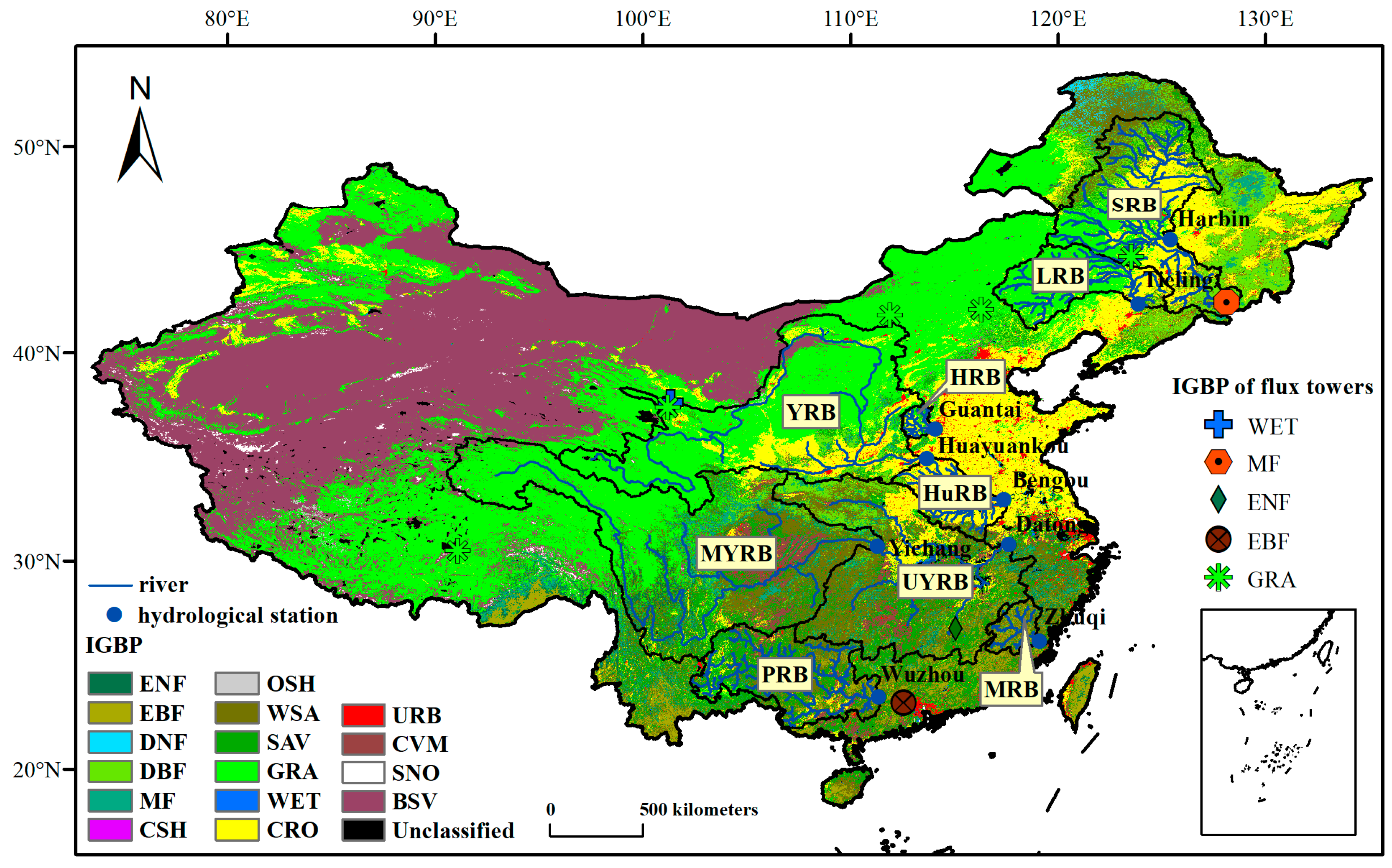
Figure 1. The spatial distribution and land use types of ten flux towers from the FLUXNET2015 dataset, as well as the spatial distribution of nine basins and corresponding hydrological stations, with basin boundaries delineated by black solid lines.
Agriculture 15 01945 g001
Figure 2. Spatial (upper triangle) and temporal (lower triangle) consistency among ET products. The R2 in the upper triangle is calculated from data of all grid points over the period 2003–2014 (annual average), measuring the consistency in the spatial distribution patterns among different ET products. We refer to this as the spatial consistency coefficient. A higher value indicates a greater similarity in spatial distribution patterns among the products. The R2 in the lower triangle is calculated from all time series data (monthly from 2003 to 2014), measuring the consistency in the temporal variation sequences among different ET products. We refer to this as the temporal consistency coefficient. A higher value indicates better agreement in temporal dynamic changes among the products. The dashed line represents the 1:1 line, which serves as a reference benchmark for a perfect fit. The solid line represents the linear regression line fitted using the monthly ET data between each pair of products, and the closer the color is to yellow, the denser the data.
Agriculture 15 01945 g002
Figure 3. Uncertainty (RMSE, unit: mm/month) of nine ET products evaluated based on the TCH method in nine major watersheds. Each bar chart represents the RMSE value of an ET product in a specific watershed, displaying the performance of different ET products in different watersheds. By comparing the performance of different products in different watersheds, the adaptability and uncertainty of the model under different geographical and climatic conditions are reflected. The colors in the picture distinguish different ET products and help identify the relative performance of each product.
Agriculture 15 01945 g003
Figure 4. Seasonal variations of relative uncertainty for nine ET products across nine basins. Each subplot represents the relative uncertainty of a specific ET product across different months, with each row corresponding to a different ET product (Gleam, REA, CLSM, etc.) and each column representing a basin (e.g., SRB, LRB, YRB, etc.). The color scale indicates the percentage of uncertainty, ranging from 0% (blue) to 40% (red). This figure highlights the temporal and spatial variability of uncertainty in ET estimation for each product under different climatic conditions across the study area.
Agriculture 15 01945 g004
Figure 5. Comparison of the estimated ET for the nine grid products with the monthly time series for calculating ET based on the water balance over the period 2003–2014. (ai) represent MYRB, HRB, HuRB, YRB, LRB, MRB, SRB, UYRB, and PRB.
Agriculture 15 01945 g005
Figure 6. Comprehensive assessment of ET products across different land cover types and monthly time series. (a) Monthly time-series variation of 8 ET products across different land cover types (monthly RMSE). (b) Performance metrics (R, MAE, RMSE, Pbias) for 9 ET products across five land cover types (EBF, ENF, GRA, MF, WET).
Agriculture 15 01945 g006
Figure 7. Comparison of estimated ET performance of four daily-scale ET products under different temperature conditions. (a) Taylor chart comparison, including RMSE, R, and standard deviation. (b) Box plot comparison, including the distribution of PBias. (c) Stacked bar chart comparison, including MAE. (1 for extreme high temperature: 0–5%; 2 for high temperature: 5–15%; 3 for ambient temperature: 15–85%; 4 for low temperature: 85–95%; and 5 for extreme low temperature: 95–100%).
Agriculture 15 01945 g007
Figure 8. Comparison of estimated ET performance of four daily-scale ET products under VPD temperature conditions. (a) Taylor chart comparison, including RMSE, R, and standard deviation; (b) Box plot comparison, including the distribution of PBias; (c) Stacked bar chart comparison, including MAE. (1 represents extreme high VPD: 0–5%; 2 represents high VPD: 5–15%; 3 represents normal VPD: 15–85%; 4 represents low VPD: 85–95%; and 5 represents extreme low VPD: 95–100%).
Agriculture 15 01945 g008
Figure 9. Comparison of MAE for 9 ET products under drought (SPEI < −1.5) and non-drought (SPEI ≥ −1.5) conditions at the site scale (1 for drought, 2 for non-drought).
Agriculture 15 01945 g009
Figure 10. The performance of the four daily ET products under extreme climatic conditions compared against observations from flux towers. (a,d,g) represent the R2, RMSE, and PBias of ET products under different temperature conditions; (b,e,h) represent the R2, RMSE, and PBias of ET products under different VPD conditions; (c,f,i) represent the R2, RMSE, and PBias of ET products under different drought conditions.
Agriculture 15 01945 g010
Figure 11. (a) Contribution rate of each input in the RF (under combination 4A); (b) standardized SHAP summary chart for Four Variables.
Agriculture 15 01945 g011
Figure 12. SHAP dependency graph of GLEAM (a), ERA5 (b), REA (c), and CLSM (d).
Agriculture 15 01945 g012
Table 1. Information on nine grid ET products used in this study.
Temporal ResolutionET ProductsSpatial ResolutionTemporal CoverageDetail LinksReference
dailyGLEAMv4.2a
(GLEAM)
0.1°1980.01–
2023.12
http://www.gleam.eu (accessed on 15 April 2025)[43]
dailyREA0.25°1980.01–
2017.12
https://data.tpdc.ac.cn (accessed on 15 April 2025)[44]
dailyCLSM0.1°2003.01–
2025.03
https://doi.org/10.5067/TXBMLX370XX8 (accessed on 15 April 2025)[45]
dailyERA5-Land
(ERA5)
0.1°1950.01–
2020.12
https://doi.org/10.24381/cds.68d2bb30 (accessed on 15 April 2025)[46]
8 daysMOD16A2500 m2001.01–
present
https://www.ntsg.umt.edu/project/modis/mod16.php (accessed on 15 April 2025)[47]
8 daysPMLv2500 m2002.01–
2017.12
https://doi.org/10.11888/Geogra.tpdc.270251 (accessed on 15 April 2025)[42]
monthlyNOAH0.25°2000.01–
2024.12
https://doi.org/10.5067/E7TYRXPJKWOQ (accessed on 15 April 2025)[48]
monthlyFLDAS0.1°1982.01–
2024.12
https://doi.org/10.5067/5NHC22T9375G (accessed on 15 April 2025)[49]
monthlySynthesized (Syn)0.1°1982.01–
2019.12
https://doi.org/10.7910/DVN/ZGOUED (accessed on 15 April 2025)[50]
Table 2. Summary of flux tower information.
Site NameLatitudeLongitudeClimate TypeLand Cover Type
CN-Cha42.4025128.0958Northeastern Humid and Semi-Humid Temperate ZoneMF
CN-Cng44.5934123.5092Northeastern Humid and Semi-Humid Temperate ZoneGRA
CN-Dan30.497891.0664Qinghai–Tibetan Plateau RegionGRA
CN-Din23.1733112.5361Tropical Humid ZonesEBF
CN-Du242.0467116.2836Inner Mongolia Grassland RegionGRA
CN-Du342.0551116.2809Inner Mongolia Grassland RegionGRA
CN-Ha237.6086101.3269Qinghai–Tibetan Plateau RegionWET
CN-HaM37.37101.18Qinghai–Tibetan Plateau RegionGRA
CN-Qia26.7414115.0581Subtropical Humid ZoneENF
CN-Sw241.7902111.8971Inner Mongolia Grassland RegionGRA
Table 3. Summary information of 9 river basins and hydrological stations.
CodeStationRiver BasinLatitudeLongitudeArea (104 km2)Periods
10701210HaerbingSonghua River Basin (SRB)45.41125.3938.981955–2014
20600200TielingLiao River Basin (LRB)42.33123.8412.081954–2014
31007000GuantaiHai River Basin (HRB)36.33114.081.781951–2015
40105150HuayuankouYellow River Basin (YRB)34.91113.67731950–2014
50104160BengbuHuaihe River Basin (HuRB)32.95117.3712.131950–2014
60107300YichangUpper Yangtze River Basin (UYRB)30.69111.28100.551950–2014
61804151DatongMiddle Yangtze River Basin (MYRB)30.78117.61701950–2014
71200500ZhuqiMinjiang River Basin (MRB)26.15119.105.51950–2014
80115000WuzhouPearl River Basin (PRB)23.46111.3332.71954–2014
Table 4. Input combinations for this study.
CombinationsInputs
1AGLEAM
1BERA5
1CREA
1DCLSM
2AGLEAM + ERA5
2BGLEAM + REA
2CGLEAM + CLSM
2DERA5 + REA
2EERA5 + CLSM
2FREA + CLSM
3AGLEAM + ERA5 + REA
3BGLEAM + ERA5 + CLSM
3CGLEAM + REA + CLSM
3DERA5 + REA + CLSM
4AGLEAM + ERA5 + REA + CLSM
Table 5. Accuracy of the 9 ET products at the basin scale.
ET ProductsRPBias (%)MAE (mm/Month)RMSE (mm/Month)
GLEAM0.864.4616.8322.94
REA0.86−2.1118.3924.41
CLSM0.803.9720.5927.04
ERA50.8621.9719.4725.86
NOAH0.8719.1119.6225.76
FLDAS0.8713.8918.2124.35
Syn0.89−2.9117.2923.24
MOD16A20.85−8.1621.5027.78
PMLv20.86−5.8918.7825.21
Note: the best statistical values for each indicator are highlighted in bold.
Table 6. Statistical metrics for machine learning under different combinations for overall and extreme climatic conditions (extreme temperature and extreme VPD include cases other than normal or conventional VPD).
CombinationsXGBGPRRFRF Under Extreme TemperatureRF Under Extreme VPDRF Under Drought
R2RMSER2RMSER2RMSER2RMSER2RMSER2RMSE
mm/dmm/dmm/dmm/dmm/dmm/m
1A0.790.540.760.510.850.410.521.120.541.100.6320.59
1B0.770.540.750.510.830.420.511.180.531.160.6321.15
1C0.750.580.740.550.820.470.511.250.511.220.6221.87
1D0.690.630.670.610.770.510.481.300.501.260.6122.32
2A0.850.470.820.430.890.340.610.890.630.870.7016.17
2B0.830.490.820.440.870.380.600.890.610.880.6916.67
2C0.830.480.810.440.880.360.590.910.610.900.6816.98
2D0.830.500.800.460.880.370.580.910.590.920.6817.64
2E0.830.490.820.450.880.360.580.920.590.920.6817.49
2F0.810.530.790.480.860.410.570.920.580.920.6718.55
3A0.860.450.850.400.900.330.700.630.720.620.7613.94
3B0.870.440.850.390.900.320.710.630.720.620.7713.60
3C0.850.460.850.400.890.340.700.640.710.620.7514.52
3D0.850.480.840.420.890.360.690.650.700.640.7415.21
4A0.880.440.870.380.910.320.720.610.730.600.8111.26
Note: the best statistical values for each indicator are highlighted in bold.
Disclaimer/Publisher’s Note: The statements, opinions and data contained in all publications are solely those of the individual author(s) and contributor(s) and not of MDPI and/or the editor(s). MDPI and/or the editor(s) disclaim responsibility for any injury to people or property resulting from any ideas, methods, instructions or products referred to in the content.