A Novel Remote Sensing Framework Integrating Geostatistical Methods and Machine Learning for Spatial Prediction of Diversity Indices in the Desert Steppe

Abstract

Accurate assessments are vital for the effective conservation of desert steppe ecosystems, which are essential for maintaining biodiversity and ecological balance. Although geostatistical methods are commonly used for spatial modeling, they have limitations in terms of feature extraction and capturing non-linear relationships. This study therefore proposes a novel remote sensing framework that integrates geostatistical methods and machine learning to predict the Shannon–Wiener index in desert steppe. Five models, Kriging interpolation, Random Forest, Support Vector Machine, 3D Convolutional Neural Network and Graph Attention Network, were employed for parameter inversion. The Helmert variance component estimation method was introduced to integrate the model outputs by iteratively evaluating residuals and assigning relative weights, enabling both optimal prediction and model contribution quantification. The ensemble model yielded a high prediction accuracy with an R² of 0.7609. This integration strategy improves the accuracy of index prediction, and enhances the interpretability of the model regarding weight contributions in space. The proposed framework provides a reliable, scalable solution for biodiversity monitoring and supports scientific decision-making for grassland conservation and ecological restoration.

1. Introduction

As key ecosystems in arid and semi-arid regions worldwide, desert steppes form transitional zones between typical grasslands and deserts. These ecosystems are typically characterized by low species diversity and potential productivity, and are often considered the limiting state of grassland ecosystems [1]. Plant diversity in these regions plays a crucial role in maintaining ecosystem stability and sustaining ecological services [2]. The Shannon–Wiener index, as a key quantitative indicator of plant community diversity, comprehensively reflects species richness and evenness. It has been widely applied in biodiversity monitoring, grassland degradation assessment, and ecological restoration [3,4,5]. In the context of accelerating global aridification and land degradation, accurately estimating the spatial distribution of the Shannon–Wiener index in desert steppe holds significant scientific value for ecosystem conservation and sustainable land management.

Traditionally, the acquisition of the Shannon–Wiener index has relied on field surveys of species composition within sample plots. While this approach is highly accurate and ecologically interpretable, it is limited by high labor costs, lengthy survey periods, and limited spatial coverage, making it unsuitable for large-scale, multi-temporal continuous monitoring. Consequently, geostatistical methods, such as Kriging interpolation, inverse distance weighting (IDW) and Spatial regression have been employed to estimate the index spatial distribution. These methods construct spatial variability models based on the spatial autocorrelation of sample plot data, allowing for the prediction of values at unsampled locations [6,7,8,9,10]. However, in ecosystems such as desert steppe, where vegetation is sparse and distributed in patches [11], the spatial structure of the diversity index is often weak. Sample plot data frequently fail to meet the basic assumption of spatial autocorrelation required by geostatistical models [12]. The mosaic pattern of bare ground and vegetation patches leads to spatial autocorrelation that is evident only at local scales, thereby limiting the accuracy of predictions based on global spatial structures [13,14]. Furthermore, traditional geostatistical methods struggle to effectively integrate multi-source data features and lack the capacity to capture the multifactorial drivers and non-linear nature of the Shannon–Wiener index [15,16,17,18,19]. Therefore, it is essential to develop inversion methods that integrate the strengths of geostatistical spatial structures with multi-source remote sensing features while supporting non-linear modelling to enhance the accuracy and applicability of spatial estimation of the Shannon–Wiener index in desert steppe.

The continuous advancement of remote sensing technology and machine learning has provided new technical support for high-precision spatial estimation of the diversity index [20,21,22]. Remote sensing data provide large-scale, multi-temporal vegetation information through multispectral, hyperspectral, and Unmanned Aerial Vehicle (UAV) imagery [23,24,25,26,27]. These data enable the extraction of multi-source information, including spectral reflectance, vegetation indices (e.g., NDVI), and texture features, effectively revealing community composition and spatial patterns [28,29,30,31,32] and offering key data support for ecological monitoring [33,34,35,36]. Machine learning algorithms can more accurately capture the spatial heterogeneity and ecological processes due to their powerful nonlinear modelling and multi-feature fusion capabilities [37,38,39,40,41]. For example, Pulakesh Das et al. successfully captured higher-order features in complex data using Random Forest (RF) and Support Vector Machine (SVM) to efficiently predict forest health indices [42]. Similarly, Hongmin Gao, Tao Zhang et al. applied 2D and 3D Convolutional Neural Networks (3D-CNNs) to effectively capture spatial continuity, thereby improving hyperspectral image classification performance [43,44]. Although these algorithms demonstrate strong capability in feature learning and multimodal data fusion, their performance relies heavily on high-quality and sufficiently large training datasets. However, in fragile ecosystems such as desert steppe, acquiring adequate training data remains a major challenge [43]. In addition, complex spatial heterogeneity and topographic variability hinder model generalization, limiting predictive stability. The black-box nature of these models further constrains the interpretability of inversion results, making it difficult to assess ecological significance [45,46,47,48]. Therefore, leveraging remote sensing and machine learning techniques in a judicious and integrative manner is imperative to overcome these challenges, ultimately enhancing both the spatial estimation accuracy and ecological interpretability of the diversity index in desert steppe.

Although traditional geostatistical methods and remote sensing machine learning techniques have distinct advantages, their applications in plant diversity index inversion remain fragmented. Geostatistical methods can effectively utilize spatial autocorrelation information, but they are limited in capturing nonlinear relationships and are constrained compared to the rich information provided by remote sensing data and the powerful processing capabilities of big data [49]. By contrast, machine learning excels at mining multi-source data features and nonlinear patterns, but tends to overlook spatial structure information and lacks interpretability [50]. As a result, existing studies struggle to achieve high-precision, continuous, and ecologically interpretable spatial inversion of the Shannon diversity index in desert steppe. Therefore, there is an urgent need to develop a comprehensive inversion model that integrates spatial structural features, multi-source environmental variables, and machine learning methods to enhance both the spatial estimation accuracy and ecological interpretability of the Shannon diversity index in desert steppe.

This study proposes a remote sensing framework for accurately estimating parameters based on existing inversion models, introducing the Helmert variance component estimation method. This framework addresses the shortcomings of conventional methods, particularly with regard to feature extraction and nonlinear pattern recognition in complex desert grassland environments.

The key contributions of this study are:

(1)

A novel remote sensing framework integrating geostatistical method and machine learning for parameter estimation was proposed, leveraging the complementary strengths of both approaches.

(2)

A new approach to evaluating index inversion models was introduced, based on calculating their relative weights using the Helmert variance component estimation method.

(3)

The spatial distribution of the Shannon index generated by the integrated framework effectively captured plant diversity patterns in desert steppe ecosystems.

The proposed fusion framework significantly enhances the accuracy of index prediction and the interpretability of the results, while also quantifying the regional contributions of individual models. It provides a solid scientific basis for ecological monitoring and sustainable management, supporting informed and precise decision-making in ecological protection.

2. Study Area and Data

2.1. Study Area

The study was conducted at the research base of the Inner Mongolia Agricultural and Animal Husbandry Research Institute (IMARI), located in Siziwangqi, Ulanqab, Inner Mongolia Autonomous Region, China (Figure 1). The site lies in the central Gegentala Grassland of south-central Siziwangqi, spanning 41°47′14″ N to 41°47′38″ N and 111°53′10″ E to 111°54′03″ E, with a mean elevation of 1500 m above sea level. The climate is classified as mid-temperate continental monsoon climate zone, marked by low annual precipitation in summer with uneven spatiotemporal distribution, strong diurnal temperature fluctuations. Average annual temperature is 3 °C, with precipitation of 260 mm sharply contrasting with potential evaporation of 2400 mm. The area experiences abundant sunshine and frequent high-wind conditions, with a mean annual wind speed of 4.5 m/s. Vegetation is typical desert steppe, sparse and short (mean height ~7 cm, coverage 18–25%). The constructive species is Stipa breviflora, with dominant species including Artemisia frigida and Cleistogenes songorica, companion species including Salsola collina, Neopallasia pectinata, Convolvulus ammanni, Kochia prostrata, and Caragana stenophylla. The study area was designated a long-term grazing ban zone within this base (red box in Figure 1c). The study area measures approximately 90 m × 510 m and covers 4.60 hm².

2.2. Data Collection and Preprocessing

2.2.1. Sample Plots Data

A total of 94 sample plots were established in a regular grid (30 m × 15 m) using systematic sampling. Plots were spaced at 30 m intervals along the fence from the southeast corner to the north, and at 15 m intervals from east to west. Each plot measured 1 m × 1 m and was bordered with 1.5 cm diameter white hollow PVC pipes to enhance boundary visibility. To facilitate vegetation surveys and data recording, holes were drilled in the PVC pipes at 10 cm intervals, and they were interlaced with white cotton threads in an ‘S’ pattern to form 100 subplots (10 cm × 10 cm). During fieldwork, a global positioning system (GPS) and an anemometer were used to record the latitude, longitude, altitude and wind speed of each plot. Vegetation surveys combined visual estimation and standard measurements to record species composition, plant abundance (clumps), average vegetation height, maximum and minimum canopy diameters, cover and canopy images. For each plot, a vertical overhead photograph was taken at the center of the plot to ensure complete coverage, as the canopy images (Figure 2). Species identification was performed jointly by two senior investigators with botanical expertise.

To comprehensively assess grassland community biodiversity, this study used the Shannon–Wiener index (hereafter the Shannon index) for quantitative analysis. The Shannon index is calculated as (1):

$$H^{\prime }=-{\displaystyle \sum _{i=1}^s\left(P_i\cdot \ln P_i\right)}$$

(1)

where H′ is the Shannon index, S is the total number of species in the community, and P_i denotes the relative abundance of the i-th species (i.e., the proportion of individuals of that species to the total number of individuals). The Shannon index integrates both species richness and evenness; thus, its value cannot be uniquely interpreted as species number, but rather reflects a combined measure of community diversity.

The Shannon index values were derived from canopy images collected during field surveys. For each plot, the relative abundance (P_i) of each species was calculated from the canopy images as the proportion of the species within the plot. Figure 3 shows the Shannon diversity index calculated for each sampling plot.

The range of Shannon index values is greater than or equal to 0. The index equals 0 when the community contains only a single species. The index increases as species richness rises or relative abundances become more even, reflecting higher biodiversity [51].

Each canopy image was matched to its corresponding location on high-resolution RGB imagery captured by DJI M300 UAV, which was then aligned with georeferenced and geometrically corrected hyperspectral images. This process ensured spatial consistency, enabling the species labels and relative abundance values derived from the canopy images to be assigned to the corresponding hyperspectral plots as reference data for model training and validation.

2.2.2. UAV Data

Considering the climate characteristics of desert grassland and the growth cycle of herbaceous plants, UAV data were acquired during the peak growth and fruiting period, from 15 July to 15 August 2024. To ensure image quality, all flights were carried out under calm or light breeze conditions (wind speed < 3.3 m/s), with clear or nearly clear skies (cloud cover < 2%), and between 10:30 and 14:00 to maximize solar elevation. A total of five UAV flights were conducted during this period. After radiometric calibration and quality assessment, the dataset with the most stable and clear spectral information was selected for subsequent analysis. The acquisition process is as follows:

(1)

Hyperspectral images of the study area were obtained using a UAV equipped with a hyperspectral imager. A standard black-and-white reference panel was calibrated before and after each flight. The main parameters of UAV hyperspectral remote sensing system are listed in Table 1.

(2)

High-resolution RGB orthophotos were captured using the DJI M300 UAV at a flight altitude of 30 m and speed of 3 m/s (Table 1). Use DJI Zhitu software to generate orthophotos covering the entire test area. These orthoimages are primarily employed for the geometric correction of hyperspectral images, as well as for determining the corresponding positions of sample points in hyperspectral images during the cropping process.

UAV data acquisition was synchronized with field surveys, and the field-determined Shannon index values served as ground truth for validating hyperspectral images inversion results.

Table 1. Flight parameters and corresponding values of the two UAV-based hyperspectral remote sensing systems.

UAV Sensing System	Optosky ATH9010W	DJI M300
Flight altitude (m)	100	30
Flight speed (m/s)	6	3
Flight time (min)	30	30
Sidewise overlap ratio	50%	50%
Spatial resolution (cm/pixel)	14.3	0.4
Spectral range (nm)	392.59–1017.81	RGB camera
Number of bands	480	3

Table 1. Flight parameters and corresponding values of the two UAV-based hyperspectral remote sensing systems.

UAV Sensing System	Optosky ATH9010W	DJI M300
Flight altitude (m)	100	30
Flight speed (m/s)	6	3
Flight time (min)	30	30
Sidewise overlap ratio	50%	50%
Spatial resolution (cm/pixel)	14.3	0.4
Spectral range (nm)	392.59–1017.81	RGB camera
Number of bands	480	3

2.2.3. Hyperspectral Data Preprocessing

The UAV hyperspectral system employed in this study uses a push-broom imaging mode, requiring the aircraft to follow an S-shaped flight path. This acquisition strategy produced narrow and elongated hyperspectral image strips. To ensure the spectral data accurately represent surface reflectance, radiometric correction was performed using ENVI software (Version 5.3). This process converts raw hyperspectral measurements into reflectance values using dark and white reference calibrations. These can be theoretically expressed as follows:

$$R={\displaystyle \frac{I_{sample}-I_{dark}}{I_{white}-I_{dark}}}$$

(2)

where I_sample is the measured intensity of the target, I_dark is the dark reference, and I_white is the white reference.

The hyperspectral images were pre-processed using ENVI and ArcGIS to generate a seamless composite covering the entire study area. This included cropping to remove unwanted borders and minimize edge artefacts, mosaicking to combine overlapping strips using feature-based alignment, and geometric correction to align the images to real-world coordinates using GPS data and ground control points. This compensated for distortions caused by UAV motion and terrain. Atmospheric correction was not applied due to the low flight altitude and the minimal effect of the atmosphere on surface reflectance. During registration, the hyperspectral images were co-registered with high-resolution UAV RGB orthophotos in the WGS 1984 UTM Zone 49N projection system, guided by ground control points and GPS measurements.

Hyperspectral patches corresponding to each 1 × 1 m plot (7 × 7 pixels) were extracted using field survey canopy photographs and high-resolution UAV RGB orthophotos as spatial references. This resulted in 94 sample datasets. The spatial resolution of the hyperspectral image is 14.3 cm/pixel. According to the pixel resolution, the residual registration error is less than 0.5 m, which is much smaller than the sample size. Therefore, the overall registration accuracy is sufficient for subsequent analysis. To reduce spectral noise while preserving the original spectral morphology, the hyperspectral data were smoothed along the spectral dimension using a Savitzky–Golay filter.

To improve the model’s generalization capabilities, the training samples were augmented using mirroring, rotation, and a ‘mask-based augmentation’ strategy. For the latter, bare soil regions identified from field survey photographs and ENVI-based image interpretation were replaced with pixels with zero values to ensure that class labels remained unaffected. Crucially, all augmentation was strictly confined to the training set, while the test set and the imagery used for final regional inference remained unchanged. This design prevents data leakage or label inconsistency, ensuring that model evaluation and mapping accurately reflect the network’s generalization performance. Following augmentation, the number of training samples increased to 376. Model evaluation was conducted using five-fold cross-validation (5-fold CV).

For model training and testing, 376 augmented samples were used. The Kriging interpolation relied solely on the 94 original samples. For Helmert variance component estimation, we combined the full-area predictions from the five models, and the accuracy of the final predictions was validated against the 94 original samples.

3. Methods

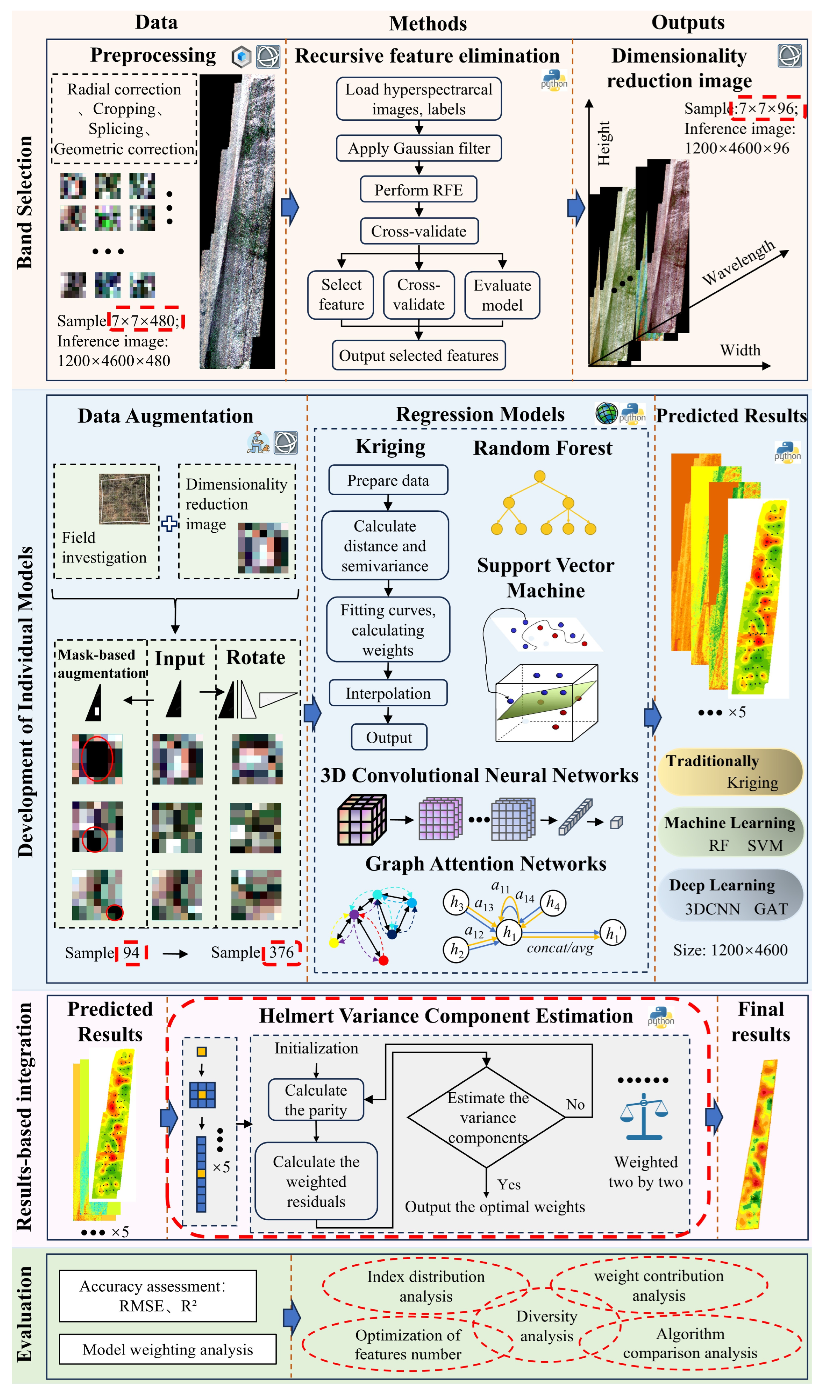
The framework includes four main steps (Figure 4). First, 96 key bands were selected from 480 hyperspectral bands using recursive feature elimination (RFE) to optimize feature inputs and improve processing efficiency. Secondly, multiple individual models were developed based on the selected bands, including Kriging interpolation, RF, SVM, 3D-CNN, and GAT, to perform the initial inversion of the Shannon index. Third, Helmert variance component estimation was applied to calculate adjustment and update weights of the model outputs, integrating their strengths to produce the most accurate Shannon index predictions and construct the spatial distribution across the study area. Finally, the accuracy and weight contribution of each model were comprehensively evaluated to quantify the contribution of each model to the final predictions, thereby providing technical support for accurate regional biodiversity monitoring.

3.1. Band Selection

The acquired hyperspectral image contains 480 bands, which contains abundant information but also considerable redundancy. It is crucial to reasonably select the optimal feature subset without altering the original feature space structure. In this study, the RFE algorithm is employed to gradually improve model performance and reduce overfitting by iteratively eliminating the less important features. A RF regressor is first used as the base model to construct a forest of 100 decision trees, and a fixed random seed of 42 is applied to ensure the reproducibility of the experimental results. Combined with recursive feature elimination with cross-validation (RFECV), one feature is eliminated in each round of iteration, and five-fold cross-validation is used to evaluate model performance. Finally, 96 bands are selected based on feature importance ranking to constitute the optimal feature subset.

3.2. Development of Individual Models

Based on the selected 96 bands, five individual models were constructed to perform the initial inversion: traditional Kriging interpolation; RF and SVM in machine learning; and 3D-CNN and GAT in deep learning. This was done to leverage the strengths of different methods in spatial autocorrelation modelling, feature extraction and nonlinear relationship learning, and to efficiently fuse multi-source information. As the 1 m × 1 m sample area corresponds to 7 × 7 pixels, the 7 × 7 pixels were used as the basic units and input into each inversion model.

To ensure robust performance evaluation and avoid potential spatial leakage, 5-fold CV was adopted for all machine learning and deep learning models (RF, SVM, 3D-CNN, and GAT). Specifically, the original 94 field plots were expanded to create 376 samples using data augmentation. These samples were then divided into five approximately equal subsets. In each fold, one subset (75 samples) was used as the test set and the remaining four (301 samples) as the training set. The final model accuracy was then calculated as an average of the five folds.

The experiments were conducted on a workstation equipped with an NVIDIA GeForce RTX 4060 Ti GPU (32 GB), an Intel i7-12700K CPU (12 cores, 3.60 GHz), and 32 GB DDR4 3200 MHz memory. The software environment included Python 3.9, PyTorch 2.1.2, and Scikit-learn 1.5.0.

(1)

Kriging Interpolation

Kriging interpolation is a spatial interpolation method based on the theory of geostatistical theory. Its core idea is to utilize the spatial correlation among known points to determine optimal weighting coefficients for unknown points, achieving an unbiased estimation with minimum variance. In this study, the latitude and longitude of 94 sample points were imported into ArcGIS Pro 10.8, and after excluding outliers, Kriging interpolation was performed to generate a forecast map of the Shannon index for the entire region.

The Kriging interpolation details are as follows:

Platform: ArcGIS Pro 10.8;

Module: Spatial Analyst Tools → Interpolation → Kriging module;

Method: Ordinary Kriging;

Semivariogram model: Spherical Model;

Nugget, Sill, Range: estimated automatically by ArcGIS;

Fitting method: ArcGIS default;

Outlier handling: manually removed;

Search radius/neighborhood: 12 nearest points.

The detailed operation process and screenshots are provided in the Supporting Materials (Figure S1).

(2)

RF

RF regression is an ensemble learning method that effectively improves prediction accuracy and reduces the risk of overfitting by constructing multiple regression trees and integrating their results. In this study, the random forest regressor implemented by Scikit-learn was used.

(3)

SVM

SVM regression leverages kernel function mapping to effectively capture nonlinear relationships in high-dimensional data and achieve accurate modeling of complex patterns. In this study, a radial basis function (RBF) is used as the kernel function to map the original data to a high-dimensional space, thereby enhancing the ability to capture nonlinear relationships and improving the separability of complex patterns.

(4)

3D-CNN

3D-CNNs can capture both spatial and spectral local features of hyperspectral data. The network constructed in this study mainly consists of a feature extraction module and fully connected regression module. The feature extraction module consists of three successive layers of 3D convolutional operations. Specifically, the first convolutional layer maps the input (1 channel) to 32 channels using a kernel size of 5 × 3 × 3 and a stride of 3 × 1 × 1. The second layer then increases this to 64 channels with the same kernel and stride, and the third layer expands this further to 128 channels. Each convolutional layer is followed by batch normalization and ReLU activation. Dropout3D (p = 0.1) is applied after the second layer to mitigate overfitting.

Following the convolutional spreading process, the extracted features are flattened and fed into the fully connected regression module. This module includes two hidden layers with ReLU activation and dropout before the features are reduced to a single dimension to output the final prediction value. In addition, an L2 weight decay of 1 × 10⁻⁴ is employed during optimization.

(5)

GAT

GAT is a graph neural network model based on the self-attention mechanism, which can adaptively learn the importance weights of neighboring nodes, thereby enhancing feature representation capability. The model constructed in this study contains a six-layer graph attention convolution structure. The input layer computes the inter-node attention weights and maps the features to a 64 × 4 hidden layer, while incorporating layer normalization to enhance stability. The hidden layer uses a four-head attention mechanism to aggregate features and introduces Leaky ReLU activation and residual connectivity to mitigate gradient vanishing and facilitate feature transfer. The output layer uses a single-head attention mechanism combined with global mean pooling to generate graph-level features.

To feed the GAT model, each 7 × 7 pixels hyperspectral patch was converted into a graph. Each pixel within a patch was treated as a node, with its spectral vector serving as the feature. This resulted in 49 nodes per patch. These nodes were then connected to their immediate neighbors in four directions (up, down, left and right) to form a regular grid graph. Edge connections were stored as an edge index tensor for PyTorch Geometric. No predefined edge weights or normalization were applied as the GAT layers learn attention coefficients adaptively. Each graph was assigned the label of its corresponding 1 × 1 m field sample plot, and the spatial position of each patch within the original image was recorded to preserve spatial correspondence.

The GAT model employs a dynamic composite loss function consisting of three terms: (i) MSE between predictions and targets; (ii) a covariance penalty term based on the sum of covariance matrix elements, weighted by a decaying factor; (iii) a Frobenius norm regularization term (λ = 0.1) applied to the covariance matrix to prevent redundancy.

$$dynamiccompositeloss=MSE+{\omega }_{\mathrm{cov}}(t){\displaystyle \sum Cov(X)}+\lambda {‖Cov(X)‖}_F$$

(3)

where ${\omega }_{\mathrm{cov}}(t)=0.001\times {0.99}^{epoch}$.

Hyperparameters and training configurations of models are shown in

Table 2. Hyperparameter values and training configurations of the machine learning and deep learning models used in this study.

Model	Architecture/Core Hyperparameter Values	Training Strategy
RF	n_estimators = 5000; max_depth = 50; min_samples_split = 20; min_samples_leaf = 10; max_features = log2; bootstrap = True.	Split criterion = MSE; bootstrap sampling enabled; ensemble aggregation by bagging; learning rate not applicable.
SVM	Penalty parameters = 500; Epsilon = 0.3; kernel = rbf; gamma = scale.	Loss function = ε-insensitive; the optimal solution is solved by convex optimization; StandardScaler fitted on each fold training subset.
3D-CNN	Conv3d layers: (1→32→64→128); with kernel sizes (5, 3, 3), strides (3, 1, 1); learning_rate = 1 × 10−4; Adam: betas = (0.85, 0.95).	Loss function = MSE; optimization by Adam; dropout + batch normalization; epochs = 200; batch size = 4.
GAT	num_layers = 6; hidden = 64; heads = 4; dropout = 0.3; learning_rate = 1 × 10−4; Adam betas = (0.85, 0.95).	Loss function = dynamic composite loss; optimization by Adam; node embeddings aggregated by global mean pooling; epochs = 200; batch size = 4.

Note: For the Adam optimizer, betas = (0.85, 0.95) denote the exponential decay rates for the first-moment (β₁ = 0.85) and second-moment (β₂ = 0.95) estimates, applied simultaneously in the moving-average computations.

.

3.3. Integrated Model (Helmert Variance Component Estimation)

To integrate the strengths of the individual models, the Helmert variance component estimation algorithm was employed. This approach quantitatively evaluates the relative accuracies of different observational data sources, determines their optimal weights, and thereby enhances the reliability and precision of the final results. With the continuous development of testing technology and artificial intelligence, the types and characteristics of observation data had been expanded from single-type to multi-type. This study assumes that the inversion results of different methods (Kriging, RF, SVM, 3D-CNN, GAT) represent five distinct levels of observation accuracy. Based on the hypothesis of environmental homogeneity, and combining the spatial resolution property of hyperspectral images (1 m corresponds to 7 pixels) with the ecological zoning information characterized by the diversity index [52,53], this study assumed that the variation in the diversity index was small within a range of 3 m (approximately corresponds to 21 pixels) and could thus be regarded as approximately uniform. The block still corresponds to 7 × 7 pixels. To optimize the accuracy assessment, the predicted values of each block and its eight surrounding blocks were taken as the measurements for that block, and then 3 × 3 matrix blocks were reshaped into column vectors so that each method could provide at least nine observations for each block.

The core principle of the Helmert variance component estimation algorithm is to estimate the variance components of each observation group based on the residual statistics after adjustment through an iterative process, and iteratively adjust the weight distribution until the unit weight variance of each observation group converges to a consistent value [54].

(1)

Workflow

Initialization: All observation groups were initially assigned an equal weighting and the unit weight variance was set at 1:1.

Iterative adjustment and convergence: Observation residuals were processed iteratively to update the variance components and adjust the weights of each group. Iterations continued until the variance ratio of the unit weights between groups converged, thereby ensuring balanced contributions. Although convergence typically occurred well before reaching this limit, a maximum iteration time of 1000 was set to guarantee termination.

Weight computation and uncertainty estimation: Once the process had converged, the final weights for each method were calculated based on the estimated variance components, with uncertainties being approximated through residual propagation.

Pairwise weighting and normalization: Pairwise weighting was conducted across all methods to determine the weights of each method’s predictions independently. These weights were then normalized to obtain the final set of weights for multi-source prediction fusion.

Interpretation: The resulting weights reflect the reliability of each method relative to the others. This provides an objective basis for combined inference and enables the effective integration of complementary information from multiple sources.

(2)

Theoretical Formulation

The implementation steps outlined above can be formally expressed through the following theoretical framework. The independent predictive weights of the two methods were determined first. The independent predictive values of the two groups of methods were organized into the test vector l and coefficient matrix B, and then the weight adjustment and variance component estimation were performed as follows:

$$l=\left[\begin{array}{c}{l}_1\\ l_2\end{array}\right],\hspace{1em}B=\left[\begin{array}{c}{B}_1\\ B_2\end{array}\right]$$

(4)

The initial value of the unit weight variance of the given two datasets was set to 1:1, the variance component vector was then formed as follows:

$${\sigma }^2=\left[\begin{array}{c}{\sigma }_1^2\\ {\sigma }_2^2\end{array}\right]$$

(5)

The observation weight matrix P was constructed. P was a diagonal matrix, with each diagonal element corresponding to the weight of its respective group. The weight was usually calculated as the reciprocal of the variance component of the group.

The normal equation was then constructed based on the least squares principle:

$$N=B^{T}PB,\hspace{1em}W=B^{T}Pl$$

(6)

The estimated value of the parameters was given by:

$$\hat{x}=N^{-1}W$$

(7)

The adjustment residuals were then calculated,

$$v=B\hat{x}-l$$

(8)

For the first and second sets of data, the weighted sum of squared residuals was computed,

$$w_1=v_1^T{P}_1{v}_1, w_2=v_2^T{P}_2{v}_2$$

(9)

Here, v₁ and v₂ are the residuals after grouping, and P₁ and P₂ are the corresponding weight matrices.

According to Helmert variance component estimation, the correction matrix S was constructed. The components of the S matrix were given by:

$$S_{11}=n_1-2tr(N^{-1}{N}_1)+tr\left({(N^{-1}{N}_1)}^2\right)$$

(10)

$$S_{22}=n_2-2tr(N^{-1}{N}_2)+tr\left({(N^{-1}{N}_2)}^2\right)$$

(11)

$$S_{12}=S_{21}=tr\left(N^{-1}{N}_1{N}^{-1}{N}_2\right)$$

(12)

Here, n₁ and n₂ are the number of predictions datasets; N is the total normal equation matrix; N₁ and N₂ are the corresponding sub-matrices for the datasets; and tr() represents the matrix trace, that is, the sum of the diagonal elements of the matrix.

The variance component vector was calculated,

$${\left[\begin{array}{c}{\sigma }_1^2\\ {\sigma }_2^2\end{array}\right]}_{new}=S^{-1}\left[\begin{array}{c}{\omega }_1\\ {\omega }_2\end{array}\right]$$

(13)

The weight matrix P was updated using a new variance component, the steps of “adjustment calculation → calculation of residuals → estimation of variance component” were repeated, until the ratio of the unit weight variance of the two observation datasets approaches 1:1, which represents the optimal weighting between the two methods.

In practice, we selected two methods at a time for variance component estimation, and determined their relative weights through this process. For example, for three models (a, b, and c), we first computed the relative weight ratio for the pair (a, b), then for (b, c), and finally for (a, c). Each pair was processed independently, and the resulting ratios were aggregated and normalized to produce the final weights. This procedure was applied to all five models in this study.

3.4. Model Evaluation and Results

Finally, two evaluation strategies were adopted to quantify each model’s role in the final integrated results. First, quantitative evaluation using traditional statistical metrics, including root mean square error (RMSE) and coefficient of determination (R²). RMSE reflects the square root of the average of the squared errors between the predicted and actual values; the lower the value, the smaller the prediction error of the model and the higher the prediction accuracy. R² is used to measure the model’s ability to explain the variability of the data, the closer the value is to 1, the better the model fit.

Secondly, the weights of the inversion models were evaluated by the Helmert variance component estimation method. This method calculates the unit weight error by iteratively determining the inversion residuals, enabling the determination of the models’ relative weights. Higher weights signify greater observational accuracy and a larger contribution to the final integrated result. The two strategies provide complementary dimensions for quantitatively evaluating model performance. One assesses overall predictive accuracy, while the other reveals the relative contributions of individual methods to data integration through weight assignment. Together, they offer a robust basis for assessing the accuracy and reliability of the final predictions.

4. Results and Discussion

4.1. Shannon Index Spatial Distribution

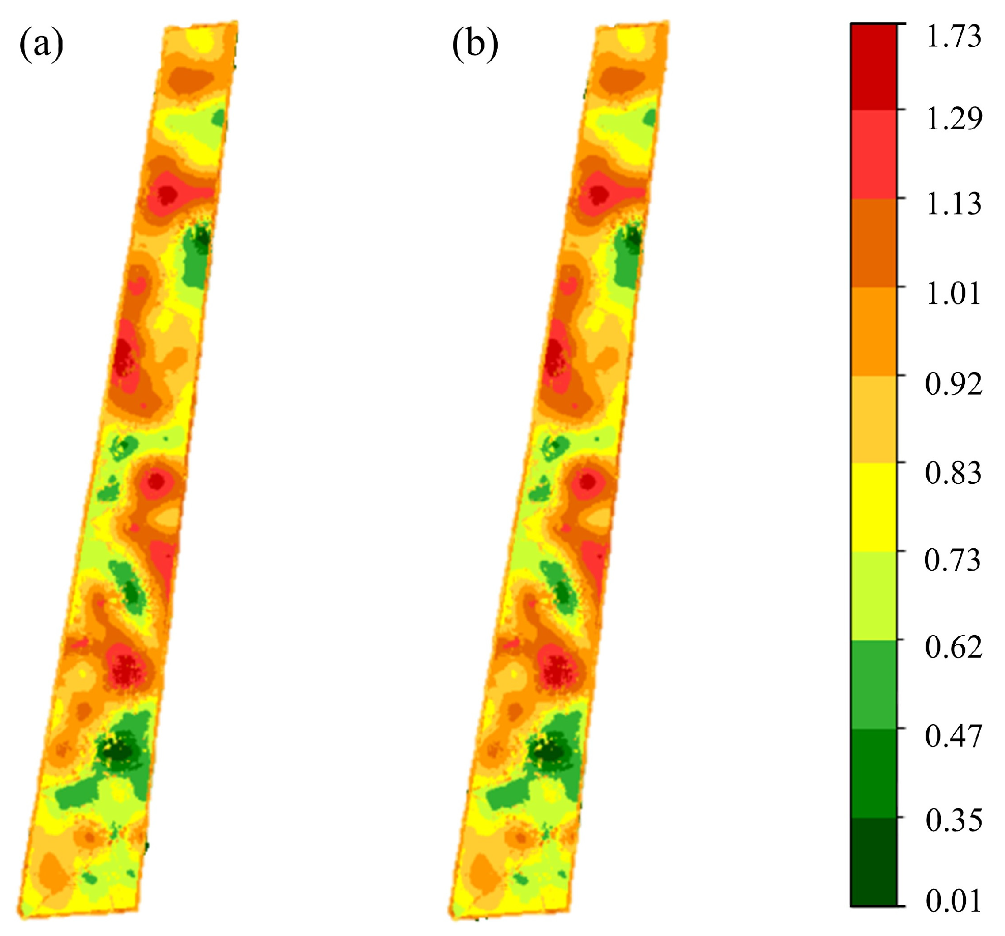
Figure 5 shows the spatial distribution of the Shannon index. The weighted median and weighted mean produced nearly identical results, with R² differing by only 0.012. It should be noted that the Shannon index integrates both species richness and evenness; thus, its value cannot be uniquely interpreted as species number, but rather reflects a combined measure of community diversity. Therefore, spatial patterns of high or low index values should be understood as the outcome of both factors rather than species count alone.

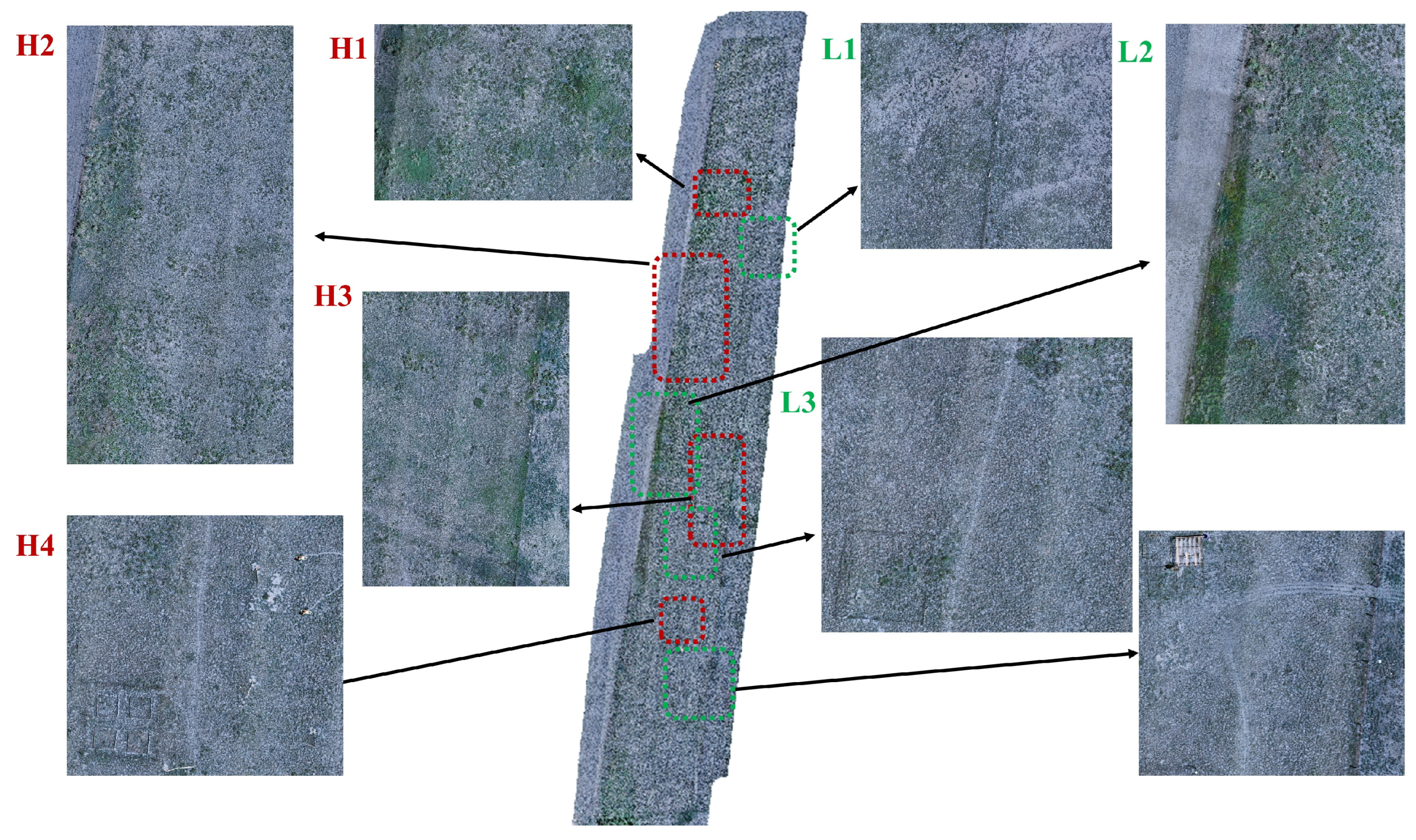
To complement Figure 5, Figure 6 serves as a contextual reference by locating these representative subregions and depicting the surrounding landscape features. While the resolution constraints of the manuscript version preclude direct identification of individual plant species, the zoomed-in panels nevertheless illustrate vegetation density and sparsity, along with observable elements such as fences, paths, and adjacent experimental plots. These contextual details provide useful background for interpreting the high and low values observed in Figure 5, thereby improving the explanatory power of the spatial diversity patterns.

The high-value zones of the Shannon index are mainly found in the northern and central regions of the study area, corresponding to zones H1–H4 in Figure 6. H1 and H2 are located in the northern region, with minimal human disturbance and no experimental facilities, resulting in relatively high indices that decrease from west to east. H3, located at the eastern boundary, is dominated by densely distributed shrubs and low herbaceous vegetation, resulting in a relatively high index. H4 lies within a fenced area with well-preserved vegetation, also exhibiting a high index. However, a 0.4 m-wide path (approximately three pixels) traverses this zone, which should theoretically lower the index, but this effect is not clearly visible on the distribution map.

The four low-index zones (L1–L4 in Figure 6) are mainly located in the south and center of the area. L1, situated along the northeastern central boundary, features sparse vegetation and a low index in its eastern section. This results from proximity to a lightly grazed area enclosed by low fences that allow sheep to graze on marginal vegetation. L2, located at the central western boundary, is primarily covered by shrubs with high canopy density but low species diversity, leading to a depressed index. L3 exhibits low, sparse herbaceous vegetation, corresponding to its low index value. L4, located near the access and the periphery of the experimental site, serves as a convergence zone for multiple footpaths. Persistent human activity in this area maintains the vegetation at a low, sparse level, resulting in a very low index.

4.2. Performance Evaluation

The spatial distribution of the Shannon index was generated by integrating predictions from all inversion models by means of Helmert variance component estimation. Model performance was evaluated at 94 sample locations, yielding an RMSE of 0.1978 and R² of 0.7609 (Figure 7).

The low RMSE (0.1978) demonstrates minimal prediction error, indicating high model accuracy. The R² value of 0.7609 reflects the model’s strong explanatory power for the diversity index of sparse vegetation in the study area. While predicted values show uniform distribution around the regression line, the slope of 0.52 reveals systematic underestimation in high-diversity zones, suggesting potential for improved inversion precision in these areas.

4.3. Weights of Inversion Models

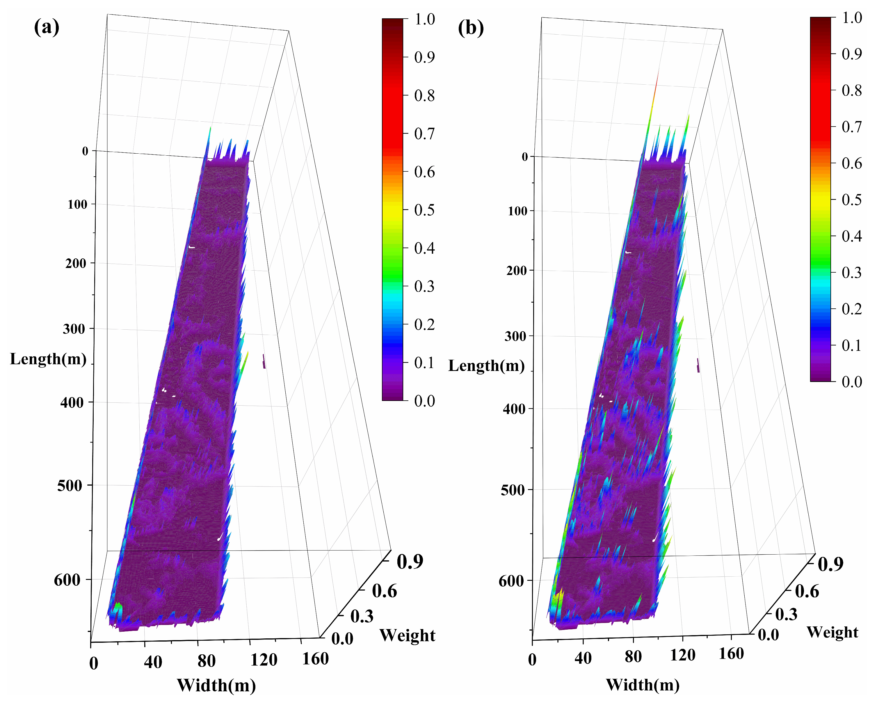
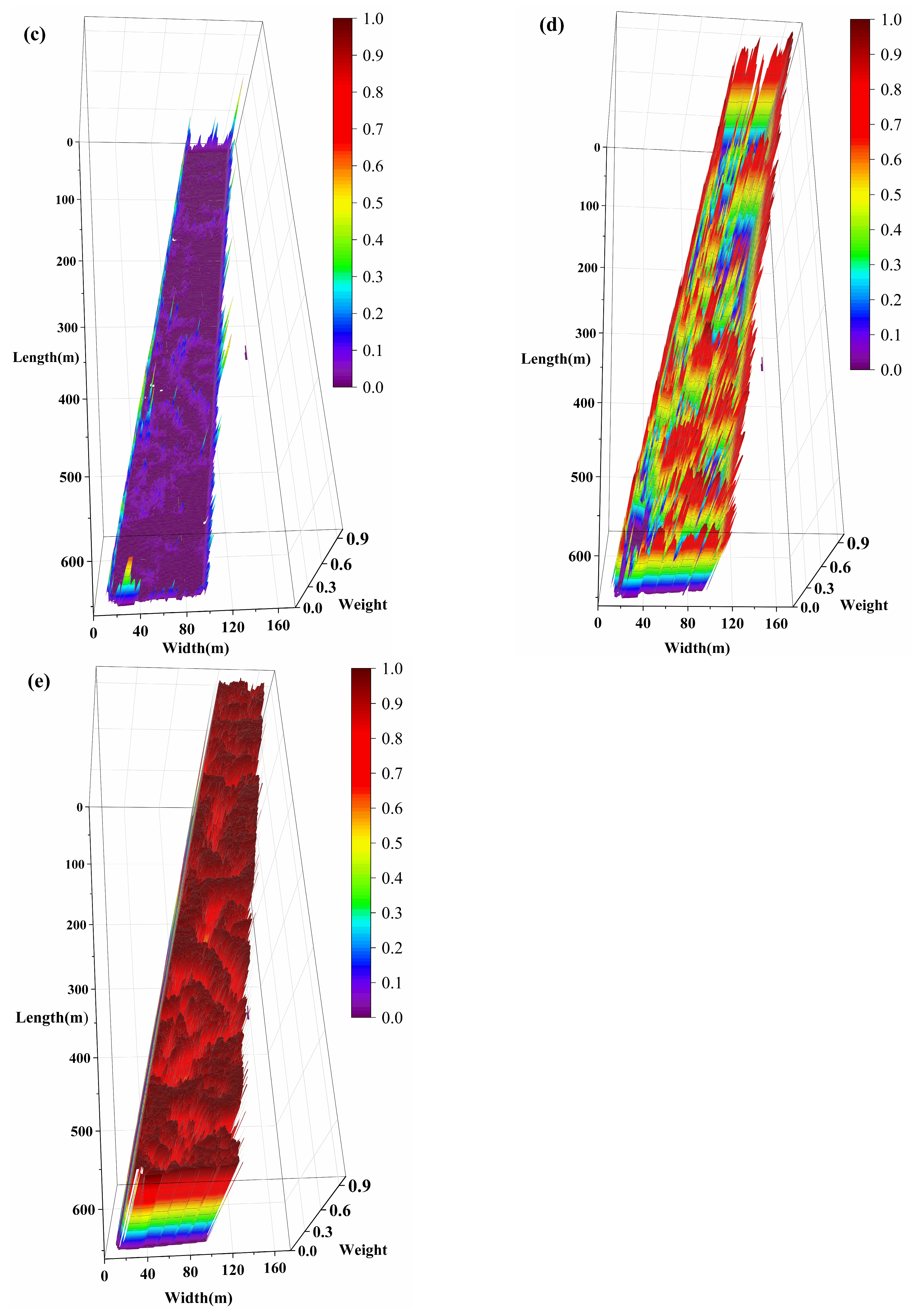
The weight contributions of the five inversion models (SVM, RF, 3D-CNN, GAT, and Kriging) in the final Shannon index prediction were determined via Helmert variance component estimation. Figure 8 presents the spatial weight distributions of different inversion models in a three-dimensional form, where the X–Y plane represents spatial locations, and the Z-axis height together with the color scale both indicate the magnitude of the model weight values. This design facilitates the identification of spatially varying model contributions and aligns with the second evaluation metric described in Section 3.4, thereby enhancing the interpretability of the results. Although a 2D contour plot could also represent the weight values, the 3D representation allows a more explicit visualization of relative differences across locations. Moreover, in the plotting software (e.g., Origin), the surfaces can be interactively rotated and zoomed, which further supports intuitive examination of model performance in spatially heterogeneous environments.

The 3D weight maps in Figure 8 illustrate the relative contributions of the five models, with all weights normalized to sum to 1. SVM, RF, and 3D-CNN show predominantly blue–purple regions, corresponding to consistently low weights across the study area. Their maximum weights are 0.3182, 0.4831, and 0.5695, while their average weights are only 0.0209, 0.0304, and 0.0222, indicating that their contributions are minor relative to the total. By comparison, GAT exhibits more yellow–red regions, reflecting moderate contributions with a maximum weight of 0.9755 and an average weight of 0.1739. Kriging dominates the weight distribution, shown as dark red–black tones, with a maximum weight of 0.9999 and an average weight of 0.7510. Together, these visual and quantitative results demonstrate that Kriging is the primary predictor, followed by GAT, while SVM, RF, and 3D-CNN contribute only marginally.

Further spatial analysis reveals that SVM, RF, and 3D-CNN weights are primarily concentrated along region boundaries (yellow-green in Figure 8a–c). Most areas are bluish-purple, with a few S-shape sky-blue bands in the center. These bands correspond to red-green junctions in Figure 5 (H2–H4, L2–L4 in Figure 6), indicating contributions of SVM, RF, and 3D-CNN in zones with significant Shannon index transitions. The GAT weight map shows high values at boundaries (red or black-red in Figure 8d). The high weights (in red) are concentrated at both the red-green intersections in Figure 5 (e.g., the intersections of H1 and L1, H3 and L2, H4 and L4) and the boundaries of the Shannon index itself (e.g., the boundaries of H2, H3 and L4). The highlights demonstrate GAT’s significant capability in capturing index mutations and boundary transitions, contributing not only at index transition zones but also at internal boundaries of high- or low-value areas. Kriging’s weight distribution (Figure 8e) aligns closely with the index variations in Figure 5, where H1–H4 and L1–L4 are clearly identifiable, blue or yellow-green weights appear only where index changes occur. About 78% of Kriging weights exceed 0.6 (red in Figure 8e), 7% are between 0.3 and 0.6 (green or yellow, Figure 8e), and 14% are below 0.3 (blue or purple, Figure 8e), confirming Kriging as the dominant predictor. It exhibits circular contours consistent with geostatistical theory, accurately reflecting the local spatial characteristics. Accordingly, the final spatial distribution of the predicted Shannon index closely resembles the Kriging pattern, primarily due to its dominant weight contribution.

4.4. Uncertainty Analysis

To comprehensively evaluate the reliability of model predictions, we conducted a systematic uncertainty analysis that combined calibration assessment, spatial residual exploration, and prediction interval evaluation. This multi-angle approach not only diagnoses the potential sources of error but also quantifies the uncertainty structure, thereby strengthening the interpretability of model outputs.

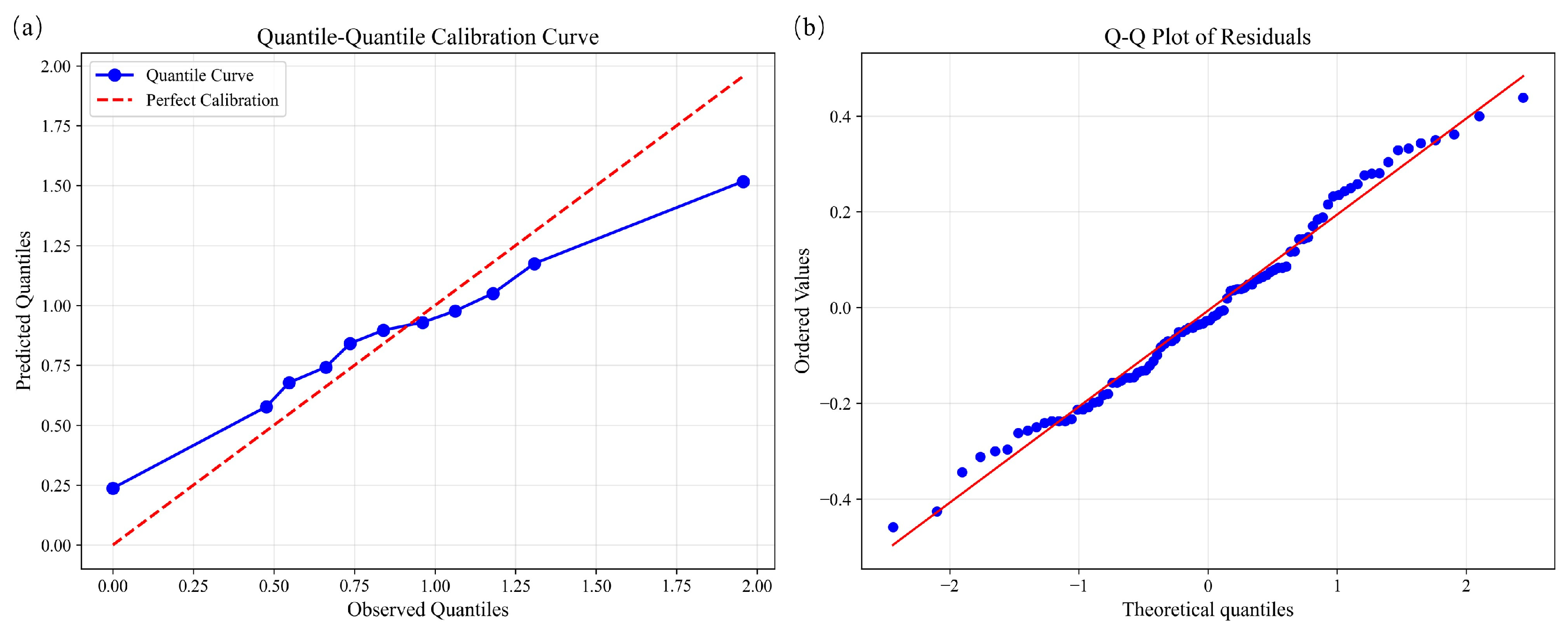
Figure 9a presents the quantile calibration curve, where the observed quantiles (blue dots) are compared against the ideal 1:1 reference line (red dashed). The curve aligns well with the reference line, particularly around the median, indicating satisfactory calibration of the model. Minor deviations at the extremes suggest a tendency of underestimation or overestimation under rare conditions. In parallel, the residual Q–Q plot (Figure 9b) shows that most points lie close to the theoretical normal distribution line, with only slight departures at both tails, confirming that residuals are approximately normally distributed.

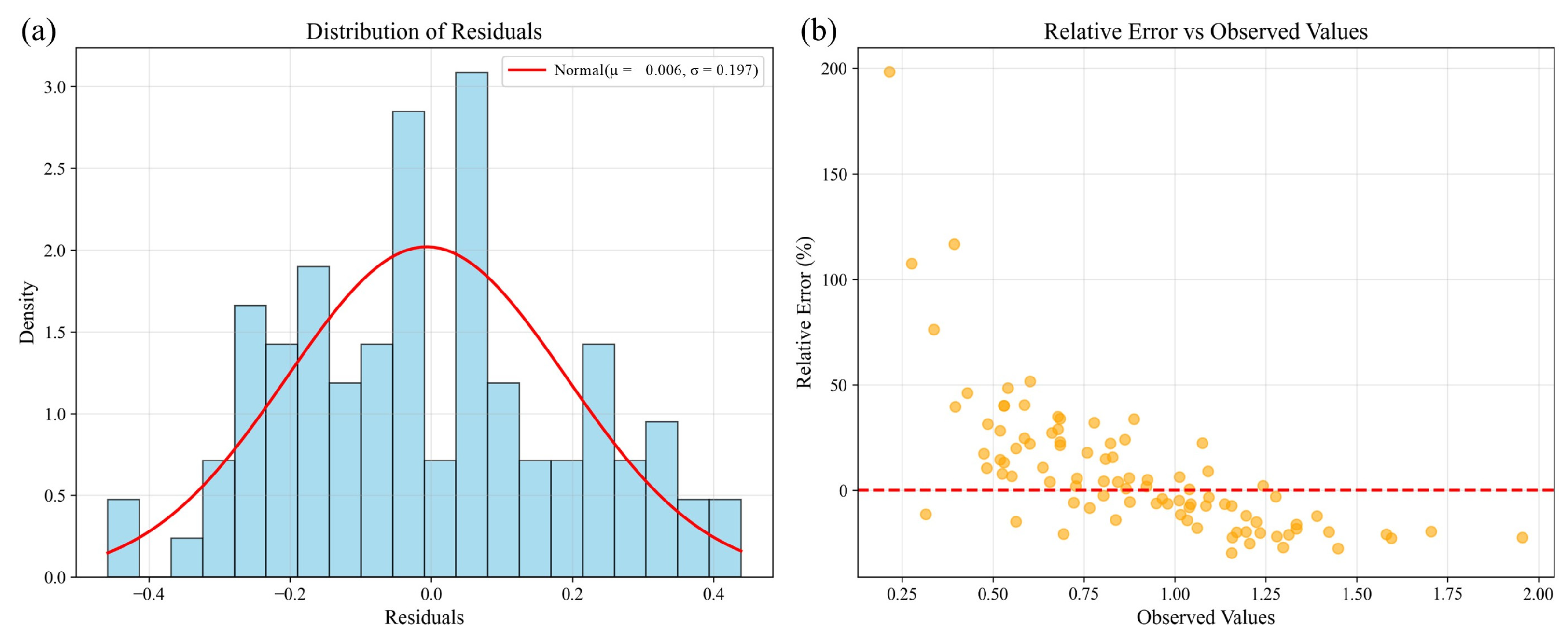
The residual histogram (Figure 10a) demonstrates a near-normal distribution centered around zero, indicating unbiased prediction errors with good symmetry. The scatterplot of relative error versus observed values (Figure 10b) reveals that most errors fall within ±50%, without clear dependency on the magnitude of observations. Larger relative errors at smaller observed values are attributable to denominator effects, a common feature in ecological data.

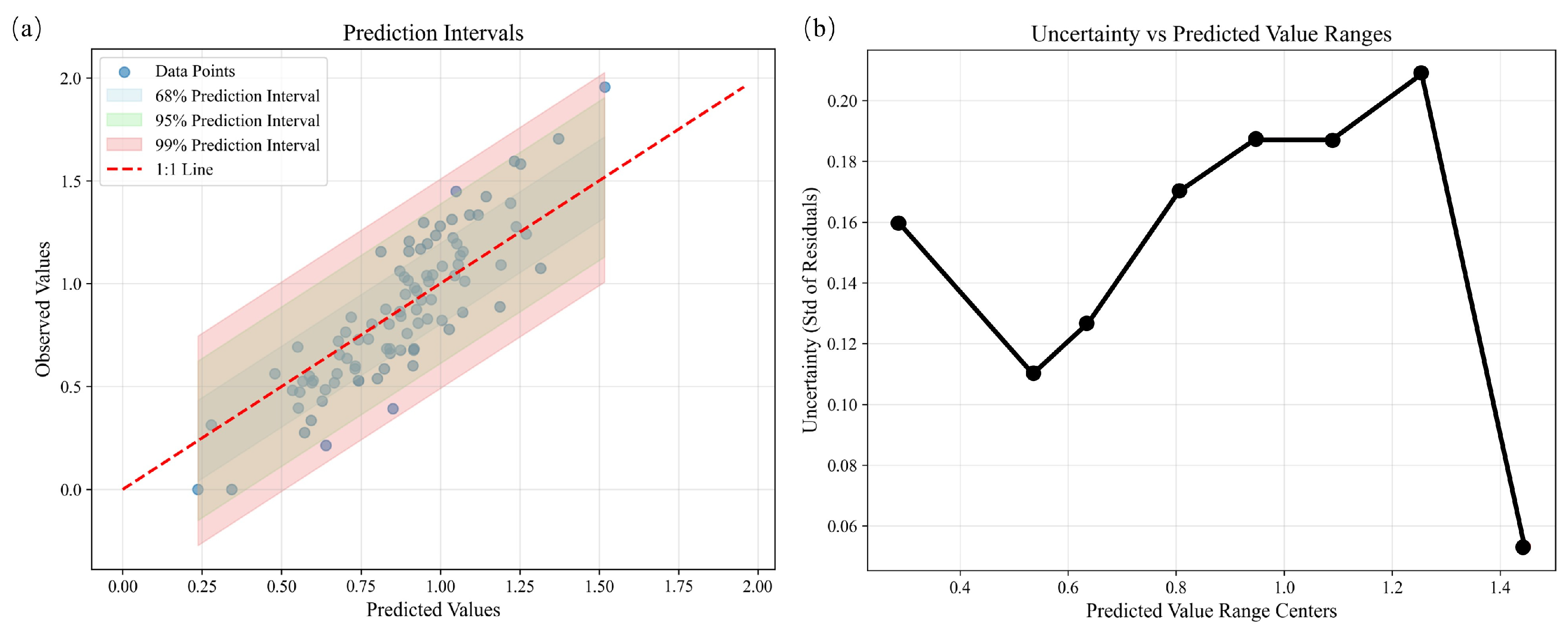
The prediction interval plot (Figure 11a) illustrates that most samples fall within the 68% (1σ), 95% (2σ), and 99% (3σ) confidence bands, suggesting that the uncertainty intervals are well-calibrated and meaningful. The uncertainty-versus-predicted-value plot (Figure 11b) reveals that uncertainty peaks in the 1.2–1.4 prediction range, potentially associated with increased ecological heterogeneity or sparse samples in this interval.

Overall, the uncertainty analysis confirms that the proposed framework exhibits good calibration, stable error distribution, and reliable prediction intervals. While residuals are generally well-behaved, the presence of slightly higher uncertainty in specific prediction ranges highlights areas where additional sampling or model refinement may further improve robustness. These findings provide confidence in the applicability of the model for ecological assessment, while also identifying directions for future methodological enhancements.

4.5. Regional Analysis of Different Index Intervals

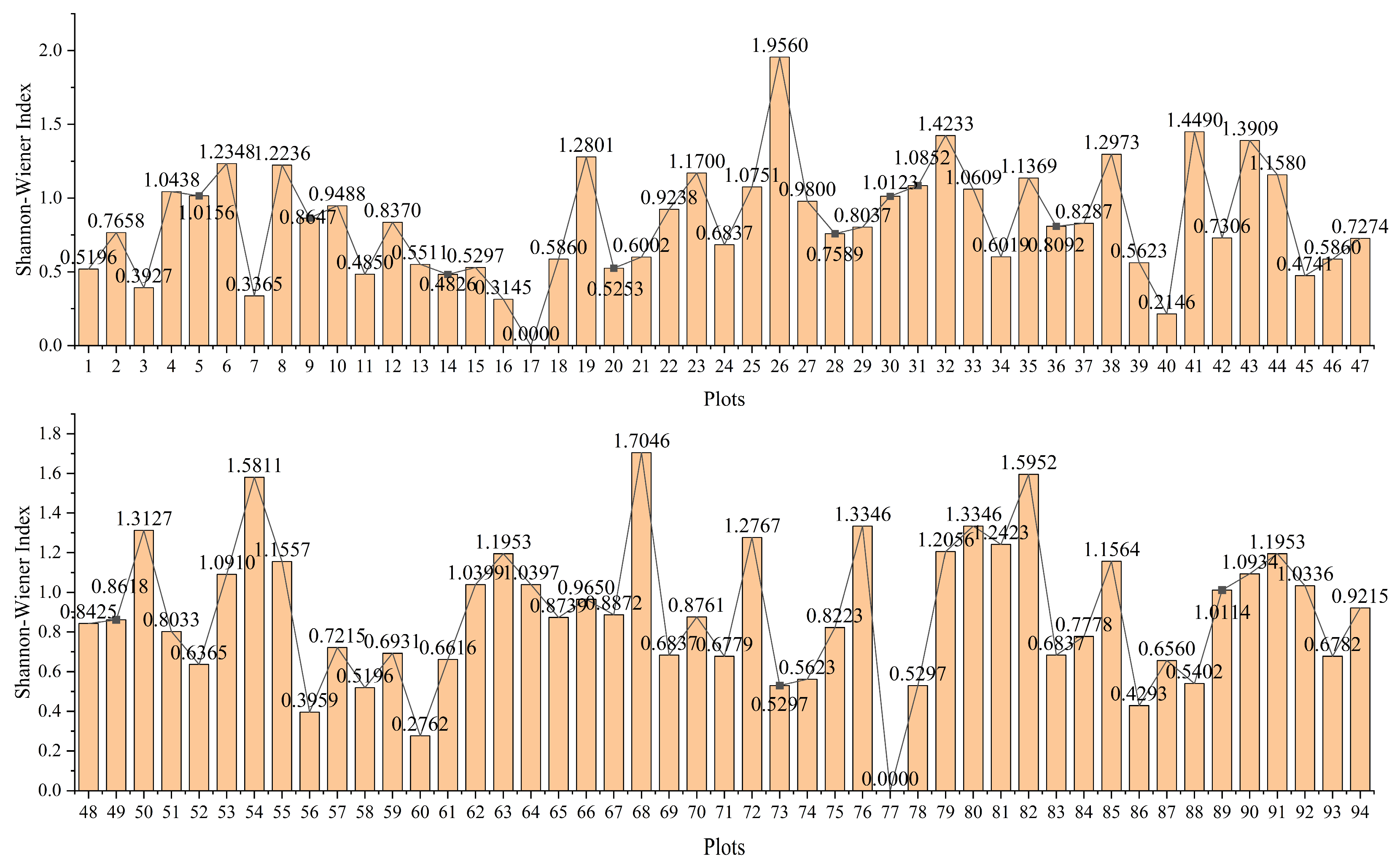
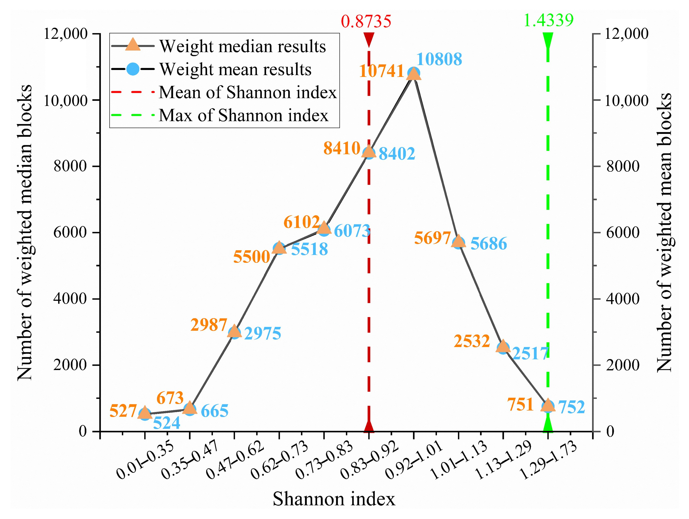
To systematically characterize the spatial distribution of Shannon index values, the number of blocks within different value intervals was tabulated (

Table 3. Number of blocks in different Shannon index intervals in the study area. The interval containing the greatest number of blocks is highlighted in bold red, while the interval containing the second greatest number of blocks is highlighted in bold black.

Type	Shannon Index Intervals
	0.01–0.35	0.35–0.47	0.47–0.62	0.62–0.73	0.73–0.83	0.83–0.92	0.92–1.01	1.01–1.13	1.13–1.29
Results based on the weighted median	527	673	2987	5500	6102	8410	10,741	5697	2532
Results based on the weighted mean	524	665	2975	5518	6073	8402	10,808	5686	2517

). The Shannon index was primarily concentrated in the 0.92–1.01 range (~10,000 blocks), followed by 0.83–0.92 (~8000 blocks). The average Shannon index was 0.8735. The class intervals shown in Table 3 are non-uniform because they were derived directly from the Kriging interpolation output in ArcGIS. Specifically, the fitted semivariogram model and the spatial autocorrelation structure of the data determine the interval boundaries. As Kriging carried the largest weight in our spatial prediction framework, these intervals naturally guided the classification displayed in Table 3 and Figure 12, while Figure 5 illustrates the corresponding spatial distribution, providing context for interpreting these stratified values.

Figure 12 shows that blocks with a Shannon index of 0 are rare, indicating that the desert grassland has not degraded into a true desert ecosystem, since areas dominated by a single species with no diversity are scarce. The maximum index value of 1.4339 indicates high diversity in certain blocks, likely resulting from an increase in adaptive species (e.g., shrubs), which enhances local species evenness and ecological stability. The mean index value of 0.8735 reflects a relatively high species diversity in this no-grazing area, although some species remain underrepresented or unevenly distributed. It is consistent with field observations, although grazing was prohibited, vegetation with high survival requirements (e.g., palatable herbaceous plants) have been declining, while adaptive species (e.g., shrubs) have become dominant species.

Figure 12 shows that the MEDIAN and MEAN curves nearly overlap, and the block count follows a normal distribution. A total of 83% of blocks had index values between 0.62 and 1.13, indicating moderate species diversity, certain distribution uniformity, presence of dominant species, and overall ecosystem stability. Approximately 25,000 blocks (57% of the total) were near the mean (0.73–1.01), indicating balanced diversity and good ecological status in more than half the region. This reflects the positive effects of long-term no-grazing policies on ecosystem protection and restoration. Notably, 22% of blocks had index values below 0.73, indicating that areas with fragile ecosystems still exist. These areas are dominated by a few species, reflecting local disturbances from external factors or environmental stress. Such lack of diversity may be linked to poor habitat conditions, invasive species, or human activities.

This approximately normal distribution of diversity values can be explained by the combined effects of multiple ecological and environmental factors. Under long-term grazing exclusion, disturbances were minimized, and ecosystem processes became more balanced, reducing extreme values. Consequently, most areas clustered around moderate diversity levels, while fewer blocks appeared at the extremes. This pattern indicates that grazing prohibition has promoted ecological stabilization, with species diversity gradually converging toward a normal distribution.

4.6. Prediction Results of Different Algorithms

The study predicted the Shannon index using SVM, RF, 3D-CNN, GAT, Kriging interpolation, and a multi-model integration method based on Helmert variance component estimation. The integrated method achieved the best performance, with RMSE = 0.1978 and R² = 0.7609, significantly outperforming the individual models (

Table 4. Prediction performance of the Shannon index using different models. The best-performing model is highlighted in bold.

Indicators	SVM	RF	3D-CNN	GAT	Kriging	Integrated Method-Mean	Integrated Method-Median
R2	0.4997	0.5398	0.5442	0.6891	0.6910	0.7609	0.7597
RMSE	0.2164	0.2543	0.2577	0.2195	0.2134	0.1978	0.1978

).

In contrast, Kriging, leveraging spatial autocorrelation, achieved higher local prediction accuracy (RMSE = 0.2134, R²= 0.6910). However, its overall performance was slightly inferior to that of the integrated method in areas distant from observed sample points because of limitations in modeling spatial variability. The deep learning models 3D-CNN and GAT achieved RMSE values of approximately 0.22 and R² values near 0.6. They demonstrated strong capabilities in feature extraction and complex pattern learning from high-dimensional data, particularly in capturing nonlinear relationships in hyperspectral data. However, their prediction accuracy remained limited in some areas with sparse vegetation and weak feature variation. Traditional machine learning models (SVM and RF) achieved R² values below 0.53 and RMSE values of approximately 0.25. These results indicate their limited ability to exploit spatial correlation and high-dimensional features, as well as an incomplete capture of potential data patterns. As a result, their prediction performance was inferior to that of the deep learning and geostatistical methods.

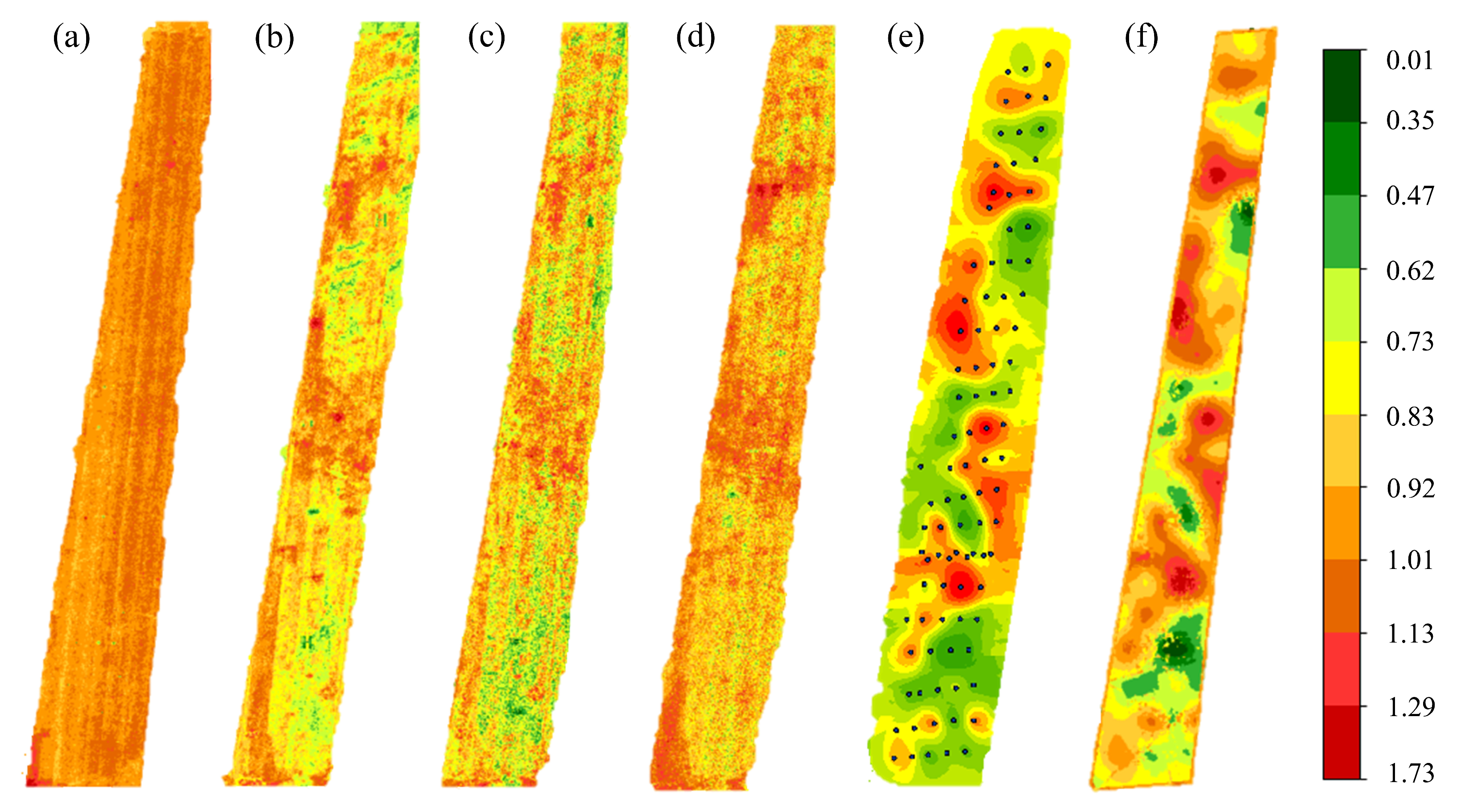
Figure 13 presents the spatial distribution of the Shannon index predicted using each method. Figure 13f shows the results of the integrated method (weighted mean) based on Helmert variance component estimation. Figure 13a (SVM) shows that the predicted values exhibit limited spatial variation, with most areas in orange-yellow and only a few sample points in yellow-green or red, reflecting the influence of training data. Figure 13b (RF) shows slightly more pronounced than in SVM, but remains largely within the yellow-green to orange range, indicating limited change in predicted values. This reflects the limited capability of traditional machine learning algorithms in handling high-dimensional data and capturing the nonlinear and spatial features of hyperspectral imagery, resulting in restricted variation in predicted values. In contrast, the predicted value variations in Figure 13c (3D-CNN) and Figure 13d (GAT) are more pronounced, with values mainly ranging from 0.5 to 0.9. Most of Figure 13d (GAT) displays yellow and orange colors, consistent with the mean prediction of 0.8735 shown in Figure 13, where 57% of plots are near the mean. The prediction results of Figure 13c,d exhibit strong spatial patterns across the study area, although local accuracy near sample points is slightly lower. This reflects the strength of deep learning models in capturing global features of hyperspectral data, which is important for enhancing large-scale prediction performance. In the prediction map of Figure 13e (Kriging), local extremes (e.g., peaks and troughs) and contour-like spatial structures are clearly visible, fully demonstrating the geostatistical model’s capability in capturing spatial continuity. However, as expected from theory, prediction reliability decreases in areas distant from the sample points.

Figure 13f presents the prediction results of the integrated method. This method leverages UAV hyperspectral data and combines Helmert variance component estimation with weighted fusion of interpolation and machine learning outputs to produce more accurate and robust parameter prediction maps. Compared to single-model prediction maps, Figure 13f displays a sharp contrast between red and green areas, clear parameter trends, well-defined partition boundaries, and data intervals, extremes, and means that closely align with sample observations. This method not only comprehensively depicts the spatial variation in the Shannon index across the study area, but also effectively balances prediction accuracy between global patterns and local details, demonstrating high practical value and applicability in desert grassland biodiversity inversion.

4.7. Selection of the Number of Hyperspectral Image Bands

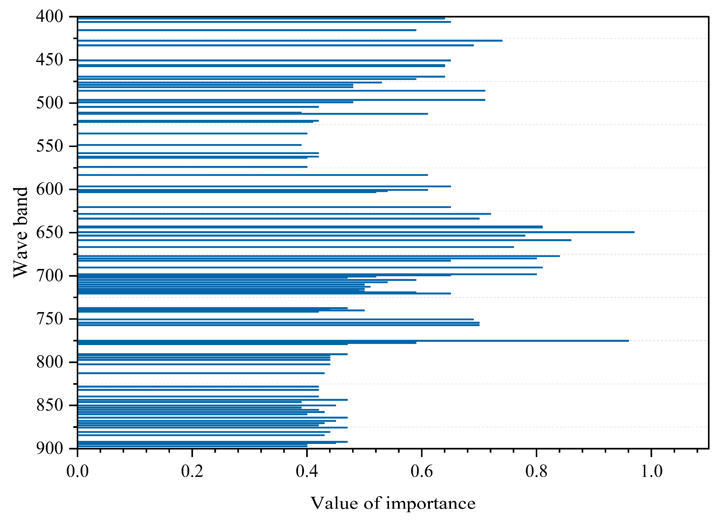
All images used for parameter inversion were derived from hyperspectral data with 480 bands. To effectively mitigate the Hughes phenomenon and improve model regression performance, recursive feature elimination (RFE) was applied using an RF regressor as the base model in conjunction with RFECV to select high-information features. The importance of all 480 bands was first computed, and multiple scenarios retaining the top 32, 64, 96, 128, and 160 bands were evaluated for prediction accuracy and computational cost. Based on these comparisons, 96 bands were selected as the optimal subset, balancing accuracy and efficiency.

The wavelengths of the selected bands are listed in Table S1, and their importance distribution is illustrated in Figure 14. Since displaying all 480 bands would be overcrowded, only the top 96 bands are shown for clarity. These bands are primarily concentrated in the red light (RL) and near-infrared (NIR) regions (around 650 nm and 760 nm), which are critical for capturing vegetation chemical composition and structural information, while some blue and green bands were retained to provide additional spectral insights.

As shown in Table S1 and Figure 14, the 96 selected bands are primarily concentrated in the red light (RL) and near-infrared (NIR) regions, with the highest importance scores observed around 650 nm and 760 nm. This indicates that the RL and NIR bands play a crucial role in reflecting the chemical composition and vegetation characteristics in plant tissue spectral analysis. The band near 650 nm is significant due to strong chlorophyll absorption of incident light, whereas the band near 760 nm corresponds to a sharp increase in reflectance, providing essential information on vegetation status. Additionally, some blue and green light bands were retained. The blue band is important given chlorophyll’s pronounced absorption in this region, as established in early vegetation index studies. The green band, with a relatively lower absorption coefficient, allows deeper light penetration into leaf tissues and multiple scattering among cell walls, thereby more effectively reflecting the structural characteristics and growth conditions of vegetation leaves.

To investigate the influence of band number on model performance, comparative experiments were carried out using the GAT model with random train–test partitioning. Unlike the previous five-fold cross-validation strategy, this simplified scheme was employed to expedite the selection of an appropriate band configuration. The corresponding results are presented in

Table 5. Prediction performance of the GAT model with different numbers of bands.

Bands	32	64	96	128	160
Calculation time (min)	10 min	18 min	27 min	36 min	45 min
R2	0.5638	0.6254	0.6700	0.6785	0.6808
RMSE	0.2397	0.2281	0.2258	0.2227	0.2142

.

The results show that increasing the number of bands improves prediction accuracy but significantly increases computational demand. For example, processing time rises from approximately 10 min at 32 bands to 45 min at 160 bands. At 160 bands, the model achieves an R² of 0.6808 and an RMSE of 0.2142. To balance accuracy and computational efficiency, 96 bands were selected as the optimal dimensionality reduction scheme.

4.8. The Prediction Results of Different Model Combinations

To investigate the impact of different model combinations on prediction accuracy, we selected five models: SVM (denoted as 1), RF (denoted as 2), 3D-CNN (denoted as 3), GAT (denoted as 4), and Kriging interpolation (denoted as 5). These models were combined in various configurations and integrated using the Helmert variance component estimation method to obtain both weighted median and weighted mean predictions. Specifically, five combinations were tested: the full combination (1–5), deep learning + Kriging (3–5), 3D-CNN + GAT (34), 3D-CNN + Kriging (35), and GAT + Kriging (45). The prediction performance of each combination is summarized in

Table 6. Prediction performance of different model combinations. The best-performing model is highlighted in bold.

Type	Indicators	1–5	45	3–5	35	34
weighted mean	R2	0.7609	0.6347	0.6321	0.6292	0.4985
	RMSE	0.1978	0.2243	0.2251	0.2258	0.3171
weighted median	R2	0.7597	0.6339	0.6310	0.6296	0.4295
	RMSE	0.1978	0.2243	0.2252	0.2257	0.3231

. The results show that the full combination (1–5) yielded the highest accuracy, with an RMSE of 0.1978 and R² of 0.7609 for the weighted mean, and an RMSE of 0.1978 and R² of 0.7597 for the weighted median.

As shown in Table 6, the full combination (1–5) achieved the highest prediction accuracy. The Helmert variance component estimation method effectively integrated the strengths of each model. By iteratively updating the unit weight error based on residuals, this method combines the feature selection and boundary delineation capabilities of machine learning algorithms with the spatial autocorrelation modeling of Kriging, leading to superior prediction results. The GAT and Kriging combination (45) achieved the second-best performance. This is attributable to the strong individual predictive abilities of both models and their complementary strengths. The integration of GAT’s graph-structured data processing with Kriging’s spatial prediction capability enhanced the extraction of deep features from high-dimensional spatial data. However, limitations in feature extraction of GAT kept the R² at around 0.63. The 3D-CNN + Kriging combination (35) showed slightly lower accuracy (R² ≈ 0.6), likely due to the complexity of 3D-CNN in high-dimensional feature processing, which increases the risk of overfitting given the limited sample size (94 samples). The 3D-CNN + GAT combination (34) performed worst (R² ≈ 0.49), reflecting the lack of complementarity between the two models in feature extraction, making it difficult to fully exploit the potential features of data.

The prediction results demonstrate that the full combination (1–5) achieves the highest accuracy, confirming the effectiveness of the Helmert variance component estimation method in enhancing parameter prediction through multi-model integration. However, this does not imply that “the more models, the better.” The effectiveness of Helmert-based integration depends primarily on the complementarity of error structures rather than the sheer number of models. Although a larger number of models were integrated (e.g., from 5 to 45 to 345), predictive accuracy did not consistently improve and in some cases even declined. This seemingly counterintuitive outcome arises because the benefits of integration hinge on how well the individual models complement one another. When multiple models share similar limitations or show poor adaptability to the characteristics of the dataset, their errors become correlated. Simply adding such models introduces redundancy or amplifies overlapping errors, thereby diminishing the advantage of integration. Therefore, improving prediction accuracy requires the careful selection of appropriate and complementary models that align with the dataset and study area characteristics, rather than indiscriminately increasing the number of models.

4.9. Overall Discussion

The parameter inversion framework proposed in this study, which integrates geostatistical methods with remote sensing machine learning, demonstrates high accuracy and stability in predicting the Shannon index in the desert grassland grazing ban area. By combining the strengths of different algorithms, the model effectively integrates spatial structural information with high-dimensional complex features, overcoming the limitations of single methods in non-linear modeling or capturing spatial variability, and significantly improving the prediction of diversity parameters. These results validate the potential of multi-algorithm integration strategies in ecological remote sensing, particularly in complex and data-sparse ecosystems.

Furthermore, using UAV-based hyperspectral imagery instead of traditional satellite remote sensing greatly enhances spatial resolution and spectral richness, enabling more precise monitoring of sparse vegetation and localized ecological changes. Combined with ground-truth samples, this approach not only provides a calibration basis for accurate mapping of hyperspectral features to ecological parameters, but also improves the model’s sensitivity to spatial heterogeneity and local microenvironmental variations, thus offering stronger support for the scientific assessment of ecologically fragile areas.

Notably, this framework is applicable not only to desert steppe but also to a variety of ecosystems such as wetlands, farmland, and aquatic environments, and can be extended to parameter inversion and environmental monitoring tasks. For example, in wetland ecological monitoring, Kriging interpolation can be used to model the spatial variability of water quality sampling points. When combined with machine learning algorithms, it enables nonlinear inversion of key spectral features from hyperspectral imagery to accurately predict water quality parameters such as chlorophyll and suspended solids concentrations. This framework offers a dynamic, high-resolution approach for monitoring diverse ecosystems, thereby providing robust support for scientific decision-making in ecological conservation, agricultural management, and resource regulation.

Although the co-registration accuracy between UAV hyperspectral and high-resolution RGB images is high, residual offsets of less than one pixel may still exist. Given the spatial resolution of the hyperspectral image is 14.3 cm/pixel, misalignment by one pixel could introduce spectral mixing at plot edges, which could affect feature extraction and model predictions. Generally, mean prediction results are relatively robust to minor offsets. However, in areas with highly heterogeneous vegetation cover, misregistration could increase local prediction uncertainty. While the overall impact is limited given that the RMSE of co-registration is <0.5 m, this potential source of uncertainty should be acknowledged when interpreting the results.

5. Conclusions and Outlook

In this study, a novel framework that integrates geostatistical methods and remote sensing machine learning is proposed and successfully applied for the spatial estimation of the Shannon index in the desert grassland grazing ban area of Inner Mongolia. The framework effectively overcomes the challenges of difficult feature extraction and complex data processing in this region. Based on hyperspectral images acquired by UAV remote sensing, 96 key bands were selected using the RFE method, which significantly optimized the feature inputs and contributed to improved data representation and model predictive performance. The Helmert variance component estimation method was applied to fuse the inversion results of Kriging interpolation, RF, SVM, 3D-CNN, and GAT, achieving optimal predictive performance with a R² of 0.7609. This framework not only significantly improves prediction accuracy and stability but also quantifies the relative contributions of different models at each spatial location, thereby enhancing the interpretability of the results. The study provides reliable technical support for the accurate monitoring and scientific management of desert grassland ecosystems, establishes a solid data foundation for ecological protection and decisions on sustainable utilization, and advances the development of ecological big data analysis methods for practical applications.

Nevertheless, there are still some limitations in this study, and future research can be extended and improved in the following directions. First, to improve the generalization ability of the fusion model, the selection and combination strategy of models should be further optimized. Future research should determine the optimal number and types of model combinations, mine the complementarity between different algorithms, and balance algorithm diversity with integration efficiency. Efficient and robust prediction schemes for various ecological scenarios can be constructed with the aid of cross-validation and hyperparameter optimization. Second, the current data mainly rely on the average reflectance values of a single-frame image, which may introduce systematic errors due to the mixed pixel effect, particularly in desert grassland regions with significant soil background. In future studies, spectral correction based on ground-truth data or the introduction of soil-adjusted vegetation indices could be considered to reduce soil background interference and improve the accuracy and reliability of diversity index inversion. These improvements would enhance the applicability and broader adoption of the model, providing stronger scientific support for dynamic monitoring and ecological protection in desert steppe and other ecologically fragile regions.