Abstract
Data-driven empirical models, including those based on reaction kinetics, are well-regarded for their ability to make accurate predictions and uncover underlying relationships. While such models have been extensively employed for microbial communities, their use in agricultural populations remains comparatively limited. In this study, researchers analyzed data from hydroponic lettuce cultivation experiments observing nitrogen-, phosphorus-, and potassium-limited growth. Dynamic μ models, which incorporated nutrient-fueled growth and maturity-based rate decay, were adapted to accommodate a variable nutrient supply, as would be expected for nutrient recovery efforts using domestic wastewater. To test these models, researchers analyzed multiple approaches, differing variations in analyses, and other agricultural models against observed biomass measurements. The resulting Dynamic μ biomass models showed significantly less error than all other tested models, were validated against three variable nutrient treatments, and were evaluated against expected wastewater concentrations. Wastewater-cultivated lettuce was predicted to grow between 20 and 72% of fresh mass compared to lettuce grown under ideal nutrient concentrations, and models identified 41.7 days to maximize dry biomass, with a final harvest time of 44.0 days to maximize fresh biomass. Finally, this research demonstrates the application of agricultural modeling for profit estimation and informing decisions on supplemental nutrient use, providing guidance for nutrient recovery from wastewater.
1. Introduction
1.1. Modeling in Agriculture
Kinetic models such as those pioneered by Michaelis-Menten and Monod have long been applied to microbial populations. The original Michaelis-Menten model from 1913 was based on enzyme-catalyzed reactions, describing how the velocity of a reaction changes with substrate concentration up to a saturation point [1,2], and has been applied to describe nutrient uptake by a population [3,4]. Then in 1941, Monod followed Michaelis-Menten to describe biomass growth during the exponential growth phase of microbial populations [5]. Since then, the Monod model and its alternatives have been applied to microbial communities, including wastewater treatment, gut microbiomes, bioremediation efforts, and biogeochemical cycles (e.g., the nitrogen cycle). Following Monod’s example, researchers have developed numerous model expansions, including those of multiple limiting nutrients [6,7], minimum nutrient concentrations [8], inhibition [9,10], and other amendments and alternative model structures.
Applying similar nutrient-driven models to agriculture, on the other hand, poses a significant challenge, as plants require much longer time periods to mature. Whereas the generation period of microbial populations may typically last between 20 min and 20 h [11], agricultural crops may grow from seed to harvest over 24–60 days (lettuce), 55–85 days (peas), and 70–100 days (tomatoes) to name a few examples [12,13,14,15,16]. These long harvest periods offer slow data collection, increase costs, and limit the quantity of data and treatments possible. This is exacerbated by the larger footprint required to grow plants, uninterrupted, over a given growth period. These represent just a few challenges influencing agricultural models, which are often categorized as either mechanistic or empirical models.
Mechanistic agricultural models saw great popularity over the past few decades and explain how biological systems operate based on fundamental knowledge of biological and physical component processes [17]. Being composed of smaller interactive components, mechanistic models excel at explaining how a system’s underlying mechanisms operate. Examples include the NiCoLet model [18], APSIM [19], and CropSyst [20], and subprocess examples include photosynthesis, respiration, transpiration and evapotranspiration, water uptake, nutrient uptake, building tissue, nutrient movement and distribution, carbon allocation, root and leaf growth, development of specialized compounds, waste products and discharge, as well as subprocesses in soil, air, and water in the plants’ environment.
While the complex understanding and flexibility provided by mechanistic models remain their strength, it also draws attention to some of their shortcomings, as they can rely heavily on assumptions and require extensive input to complete complex equations [17,21]. These inputs can include environmental conditions (e.g., CO2 concentrations, photosynthetically active radiation (PAR) light intensity, and air temperature), plant size measurements (e.g., leaf area index, root length, and root area), and plant photosynthetic response measurements. Furthermore, building these models requires large quantities of high-quality data covering a breadth of diverse conditions, in order to elucidate a large number of parameters [22], making mechanistic models ideal for machine learning and artificial intelligence initiatives [23]. However, the absence of such datasets represents one of the significant gaps in modern agricultural research.
Experimental research into specific mechanistic models has demonstrated limited accuracy and recurrent issues, including crowding (canopy closure), accuracy under varied temperatures, scalability issues when translating from small laboratory-scale to commercial-scale applications, failures in validation against experimental data, and significant overestimation of nutrient uptake in high nutrient conditions [22,24,25,26].
Meanwhile, some modeling efforts, such as those by Silberbush [27], take a hybrid approach between mechanistic and empirical approaches, taking advantage of the benefits offered by data-driven experiments. These data-driven empirical models excel at making predictions and identifying relationships, albeit without explanation of causal mechanisms. Of these, kinetic models are sometimes considered purely empirical and at other times are considered to fall between empirical and mechanistic, as they quantify relationships through analysis of experimental data while being founded on chemical and physiological processes [28]. A significant benefit of kinetic models is their increased utility, allowing users to make predictions on nutrient uptake and plant biomass growth based on relatively few and non-invasive inputs (e.g., analyzing water samples). Furthermore, they can still be incorporated into larger mechanistic or hybrid models.
The parameters for these models not only reflect their environment, but also reflect how researchers measured and calculated parameters [29]. For example, even within the scope of nitrate uptake by lettuce, Michaelis constants Km in the literature range from 0.098 to 4.956 mg-N L−1, spanning nearly two orders of magnitude [29,30,31,32]. This variation in parameter values can be partially attributed to decreasing relative growth rates (RGR) [32,33,34,35], and nutrient uptake rates [30,36] observed in lettuce, corn, and multiple tree species. These observed decreases seemingly contradict the previously held assumption from Monod kinetics that the specific or relative growth rate remains constant during the exponential growth phase. To resolve variation in observed RGR attributed to plant age, the Dynamic μ model characterizes this decreasing RGR as plants mature [37]. This solution may reconcile variation across studies which base measurements on differing growth periods while simultaneously reducing error and improving the applicability and utility of agricultural kinetic models.
While many of these kinetic models are often based on singular limiting nutrients using treatments that aim to maintain constant nutrient concentrations, such environments are not a fair representation of many water sources. This is especially true in the context of nutrient recovery from domestic wastewater, where models must be able to adapt to a variable nutrient supply and make predictions under a variety of limiting nutrients. Of the 17 essential nutrients required for plant growth, the commonly accepted most important nutrients are nitrogen (N), phosphorus (P), and potassium (K) [38,39,40]. The concentrations of these found in domestic wastewater vary significantly, with studies having identified ranges of 30–60 mg L−1 nitrogen, 5–20 mg L−1 phosphorus, and 5–40 mg L−1 potassium [41,42,43].
1.2. Research Objectives
This manuscript builds upon the Dynamic μ kinetic models observing the hydroponic cultivation of Bibb Lettuce (Lactuca sativa) in N-, P-, and K-limited conditions [37,44]. Rather than optimizing the relative growth rate (RGR, μ) via Dynamic μ, this study optimizes the prediction of fresh and dry plant biomass, and piecewise builds this biomass to simulate a variable nutrient supply. The resulting analysis will compare predicted and observed biomass measurements across treatments and alternative models, validate parameters against three variable nutrient treatments, identify optimal harvest dates as a function of nutrient supply, and quantify expected fresh and dry biomass of lettuce cultivated across the range of N-P-K concentrations found in reclaimed domestic wastewater.
2. Materials and Methods
2.1. Experimental Configuration
During each treatment, plants were cultivated in vertical nutrient film technique (NFT) hydroponic systems within environmental control chambers maintained at 21.5 °C and 50–70% relative humidity. Plants were lit with LED light bars (Infinity 2.0 LED; Thrive Agritech, Claymont, DE, USA) over a 12 h photoperiod and received a daily light integral of 14.69 ± 0.06 mol m−2 d−1, within the optimal range of 14–17 mol m−2 d−1 for Bibb lettuce [13,45]. Nutrient concentrations were maintained consistent with Modified Sonneveld Solution [38], while each target nutrient (e.g., N, P, or K) was individually raised or lowered in order to collect data supporting the influence of each respective target nutrient. A more detailed account of the experimental configuration can be found in the methodology of the cited literature [37,44].
2.2. Foundational Modeling
Modeling was duplicated from Sharkey et al. [37,44] except where otherwise indicated. Table 1 outlines applicable biomass equations from these articles.

Table 1.
Select equations from prior studies.
For foundational Monod models, an objective function was defined as the sum of root mean squared errors (RMSE) across all treatment and nutrient conditions and was minimized using the L-BFGS-B algorithm in Python 3.10.13 using the scipy.optimize module [46].
A similar approach was performed for Dynamic μ, instead utilizing the Trust Region Reflective algorithm and minimizing the sum of squared residuals. Parameter bounds were defined to reflect biologically realistic limits and improve convergence. For example, lower bounds for μmax and Ks values were set to 0 to ensure values remained positive. Delay period d was constrained to less than the life of the plant. And upper bounds for other parameters were constrained to within 3–5 orders of magnitude of expected results. This allowed significant freedom for the model to optimize without defaulting to unrealistic outputs.
2.3. Modeling Dry Mass in Dynamic μ
Equation (1) integrates and algebraically manipulates Dynamic μ (Equation (S6)) in order to estimate dry mass DM based on kinetic parameters, plant age t, and lifetime average nutrient concentration [SN].
Kinetic parameter μmax describes the maximum relative growth rate. Substrate affinity constant Ks represents the concentration of the limiting nutrient, which approximates half the maximum relative growth rate. Maturity constant m quantifies the rate at which the relative growth rate decreases as plants mature, and delay period d indicates the seedling time during which plants do not experience maturity-based decay in relative growth rates.
2.4. Modeling DM with Localized Variable Nutrient Concentrations
This Dynamic μ biomass model, Equation (1), as well as the parallel Monod model, Equation (S4), provided the foundation for a more granular approach, which piecewise implemented the influence of nutrient concentration measurements to actively predict plant biomass as the crops grew and matured.
To update these two equations from lifetime to localized measurements, researchers present a few redefined variable terms. Whereas lifetime models observed changes between t0 and t, localized measurements observed changes between tn−1 and tn, including dry mass (DMn−1 and DMn) and [Sn], which represents the mean of [S] between tn−1 and tn. This divides the model into distinct periods, delineated by water samples, each individually operating under the constant nutrient concentration assumption required for an analytical solution. The resulting dry mass, DMn, of each distinct period can be used as the following period’s initial dry mass DMn−1, thus allowing a model that can iteratively build dry mass based on changing nutrient concentrations.
Equation (2) applies these changes to predict dry mass DMn for the foundational Monod as a function of these updated parameters.
Meanwhile, Equation (3) implemented a bounded integration of the Dynamic μ model (Equation (S6)) to similarly model dry mass DMn. This bounded equation presents three cases: pre-delay, mid-delay, and post-delay. However, the post-delay equation (case #3) inherently includes the intra-delay equation (case #2), as tn−1 − d from case #3 must remain non-negative and is equal to 0 when tn−1 < d.
2.5. Multi-Nutrient Models
Of course, during practical applications, users are unlikely to be aware of which nutrients are most limiting, even when provided measured nutrient concentrations. As such, a robust model should accept multiple nutrient inputs. The extended Monod Multi-Nutrient (MMN) model, Equation (4), incorporates the effects of multiple limiting nutrients. This presentation of Equation (4) divides growth rate into fundamental components for each nutrient, exemplified separately in Equation (5), which defines the fractional contribution for each nutrient i towards reducing RGR below the maximum. These fractional contributions were expected to be high at nearly 100% in the majority of expected conditions, but their minor shortcomings would compound with those of other limiting nutrients, as well as further compounding over time as biomass grows at ever-reduced rates.
This Monod Multi-Nutrient model was then used to develop a dry mass Monod model based on multiple localized nutrient concentrations, as shown in Equation (6).
Similarly, Equation (7) defines the Dynamic μ multi-nutrient model, and Equation (8) presents the dry mass Dynamic μ model based on multiple localized nutrient concentrations.
These adapted models allow application to validation treatments and real-world applications, both in which the identity of the most limiting nutrients is uncertain. Of course, these multiple nutrient models only observe nitrogen, phosphorus, and potassium, but the framework can be easily adapted for any active-uptake nutrients in which researchers have identified kinetic parameter Ks to describe the relationship between a specified nutrient and crop species. Essential nutrients with passive uptake components (e.g., calcium) may break from this model.
2.6. Choosing How to Model: The Fit to μ Approach vs. the Fit to Mass Approach
One fundamental decision when developing a best-fit model is choosing which error to minimize. Researchers identified two approaches: the Fit to μ approach and the Fit to Mass approach. These two, and their distinctions, are defined as follows.
In the Fit to μ approach, researchers minimize error between predicted (e.g., Equations (S1) and (S6)) and observed values of relative growth rate μ. In the Fit to Mass approach, researchers minimize error between predicted (e.g., Equations (6) and (8)) and observed values of dry mass DM.
The biggest distinction between these two approaches is in data point weighting. Please note that within this section, the term weight is not akin to a mass measurement, but rather to the relative nature of multiple values against each other.
Fitting to dry mass weighs matured lettuce more heavily, as the absolute biomass of these matured plants is significantly larger. Due to exponential, or pseudo-exponential, growth, this weighting is the most significant distinction. This greater weighting is only indirectly influenced by nutrient concentrations, as lesser nutrients will grow plants with lesser biomass, resulting in lesser relative weight. For these reasons, fitting parameters to mass would be useful and preferred if larger matured plants have more value than young ones, as is often true within the field of agriculture.
On the other hand, fitting to growth rate shows no direct bias in regard to small or large biomass plants. Furthermore, plants receiving comparatively lesser nutrient concentrations are more evenly balanced when the Ks values are particularly low (e.g., relatively sharp and flat Monod curve), as was found with lettuce. However, as prior research demonstrated that RGR decreased as plants matured via Dynamic μ [37], this would indirectly result in the youngest plants being weighed more heavily than matured plants exposed to the same nutrients. This issue is exacerbated by increased noise and variability seen in younger plant samples. So while fitting to growth rate may be more stable across all nutrient concentrations, it is far from unbiased and is likely biased against the best interests of farmers and researchers seeking to maximize model utility for matured plants.
So while prior studies fit parameters to μ in order to compare growth rates, this study applied similar curve fitting methodology to optimize parameters and analyze the results of plant dry mass.
2.7. Reliant vs. Simultaneous Multi-Nutrient Models
The incorporation of multiple nutrients permits a choice between two distinct methods for identifying model parameters. These two methods, titled the Reliant Multi-Nutrient method and the Simultaneous Multi-Nutrient method, and their distinctions, are described here. Resulting parameters from either method can be applied to either foundational Monod or Dynamic μ models. This study will focus on Dynamic μ based on its improved predictive capabilities.
The Reliant Multi-Nutrient method is the most straightforward. This approach first uses a single-nutrient model (e.g., Equations (2) or (3)) to independently derive kinetic parameters for each limiting nutrient. These kinetic parameters are then collectively inserted into a multi-nutrient model (e.g., Equations (6) or (8)). Beyond being the most straightforward, this approach exemplifies combining parameters from multiple separate research publications. When doing so, ideal circumstances (e.g., well-designed and executed experiments) would be expected to yield ideal results. However, this draws attention to the unnecessary assumption that each kinetic parameter was derived absent of other nutrient limitation. This assumption can be circumvented via the Simultaneous Multi-Nutrient Model.
The Simultaneous Multi-Nutrient Model presents a more complex, yet more robust option. It accepts all inputs, from all nutrients, to solve for all kinetic parameters simultaneously using a multiple nutrient model (e.g., Equations (6) or (8)). Fortunately, modern computers have no difficulty with the complexity of a multitude of inputs nor solving for multiple parameters simultaneously.
Applying these two methods to the Dynamic μ model will result in the Reliant Multi-Nutrient Dynamic μ (RMND μ) and Simultaneous Multi-Nutrient Dynamic μ (SMND μ) models. For example, the SMND μ model will solve for parameters , , , , m, and d simultaneously, following a Fit to Mass approach (Equation (8)). To identify the parameter values that offered the best fit via this SMND μ model, researchers employed a Generalized Reduced Gradient nonlinear solving algorithm to minimize the RMSE between predicted and observed values. This was selected due to the algorithm’s smooth nonlinear model employed for the continuous nature of research parameters.
2.8. Modeling Fresh Mass
In the same manner as was performed for dry mass DM, fresh mass FM was analyzed via the Monod Multi-Nutrient model (MMN) (Equation (6)), as well as RMND μ and SMND μ models (Equation (8)). This was accomplished by implementing plant fresh mass FM in place of dry mass DM in these and all supportive equations outlined throughout the methodology. It should be understood that fresh mass parameters will exhibit values differing from those associated with dry mass, partially explained by the non-constant dry mass percentage DM% that decreases as plants mature. This fresh mass model brings applicability from engineers to farmers, who often sell their products based on the fresh mass (lbs or kgs) of their produce.
2.9. Peak Biomass Harvest Period (via Dynamic μ)
One beneficial feature of the Dynamic μ model is that it allows researchers to identify the time at which plant decay surpasses growth. By setting the relative growth rate μ at 0, researchers can algebraically manipulate Dynamic μ (Equation (S6)) to produce Equation (9). This expresses time t as a function of each individual nutrient concentration [SN] and identified kinetic parameters. While this represents a single-nutrient equation, its accuracy relies on the validity of the identified parameter values. As such, researchers used parameter values derived from the SMND μ model.
In Equation (9), time tmax represents what can be interpreted as the recommended harvest time to achieve peak biomass. After this time, each plant’s decay rate surpasses its growth rate, and prolonging harvest beyond this age will be expected to result in smaller plants. While economic, social, or biological pressures could influence an earlier harvest, there is less support for extending plant harvest beyond this date for a given limiting nutrient concentration.
2.10. Validating Models
After utilizing the SMND μ models to identify parameter values for both dry mass and fresh mass from localized nutrient concentrations of N, P, and K, these parameters were applied to the same SMND μ models using localized nutrient concentrations from three validation treatments, which had received irregular and variable nutrient concentrations. The results were compared against observed dry mass and fresh mass measurements from each treatment.
3. Results
3.1. Foundational Monod and Dynamic µ Models (Fit to Mass)
Figure 1 presents the foundational Monod models, using a Fit to Mass approach. Not only do younger plants, shown as green dots, exhibit a greater growth rate than mature individuals, but they also express greater variability between samples.
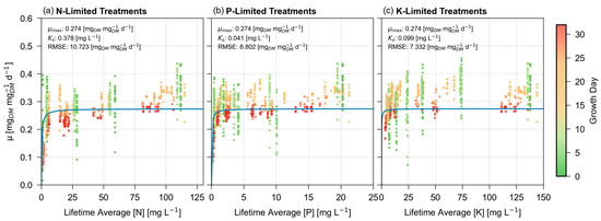
Figure 1.
Foundational Monod (Fit to Mass) model; visually exemplifying the disconnect of quantifying µ when the model is fitted to mass. Blue lines represent the model, with dots representing lifetime relative growth rates, expressed as a gradient based on the growth day of the plant at the time of harvest.
When Figure 1 is compared to the same model using a Fit to µ approach [37], kinetic parameters decrease: µmax is reduced from 0.315 to 0.274 , and Ks values reduce from 1.724, 0.225, and 0.915 mg L−1 for N, P, and K respectively down to 0.378, 0.041, and 0.099 mg L−1.
Furthermore, the RMSE increases substantially from 0.038, 0.034, and 0.034 for N, P, and K up to 10.723, 8.802, and 7.332. This increase is intuitive and expected as Monod displays changes in growth rate, so optimizing the fit for growth rate will always exhibit reduced error in comparison to optimizing the fit for biomass.
Likewise, Figure 2 illustrates the Dynamic µ model when fitted to dry mass and exhibits a closer match to its prior Fit to µ counterpart than was seen with foundational Monod.
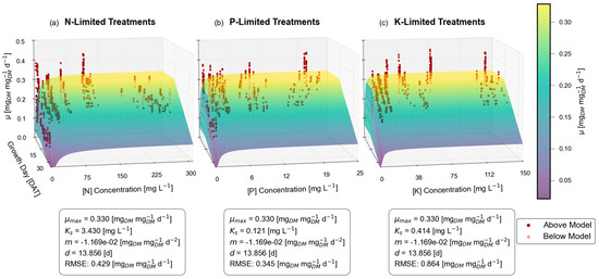
Figure 2.
Dynamic μ (Fit to Mass) model; visually exemplifying the disconnect of quantifying µ when the model is fitted to mass. The sloped plane represents the single-nutrient Dynamic µ model, with red dots representing individual lifetime average μ calculated from harvested plants.
The maximum relative growth rate µmax is not significantly affected, shifting slightly from 0.324 to 0.330 , while delay d shifts from 14.548 to 13.856 days. Meanwhile, the substrate affinity constant Ks values of 1.257, 0.168, and 0.449 mg L−1 for N, P, and K are updated to 3.43, 0.121, and 0.414 mg L−1. And while the majority of parameters only exhibit minor differences, the new approach displays a much greater maturity constant m, which became exaggerated by a factor of 3.06× from −0.00382 to −0.01169 . This exaggerated maturity constant m results in a steeper Dynamic µ model curve, approaching zero near each experiment’s conclusion on 32 DAT.
Once again, as expected, the RMSE increases from 0.026, 0.030, and 0.031 for N, P, and K when fit to growth rate, up to 0.429, 0.345, and 0.864 when fit to dry mass.
3.2. Integrated Dry Mass Models
Figure 3 presents the Integrated Dry Mass models compared against observed dry mass in each treatment, aligning dry mass measurements with a model optimized for predicting dry mass.
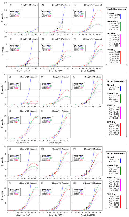
Figure 3.
Integrated Dry Mass models, with (a–f) representing N-limited treatments, (g–k) representing P-limited treatments, and (l–q) representing K-limited treatments, with each treatment labeled appropriately. Colored lines represent models: Monod Multi-Nutrient (solid blue), single-nutrient Dynamic µ (dashed green), Reliant Multi-Nutrient Dynamic µ (dotted magenta), and Simultaneous Multi-Nutrient Dynamic µ (solid red), and individual plant dry mass observations (black dots).
Not surprisingly, the foundational Monod curves increase exponentially and indefinitely in all treatments. Meanwhile, the Dynamic µ, Reliant Multi-Nutrient Dynamic μ, and Simultaneous Multi-Nutrient Dynamic μ dry mass models peak and decrease shortly after 41 DAT. Of these four models, the SMND μ model most often offers the lowest error (best fit), even improving upon the single nutrient Dynamic μ model. Due to the differing scales of biomass and differing quantities of samples between treatments, it is important to note that RMSE can only be fairly compared within each treatment, and not compared across different treatments.
Identical methods were conducted for fresh mass, and Integrated Fresh Mass Models can be found in Supplemental Information Figure S1. These fresh mass model results show even greater support than those seen in Figure 3’s dry mass model, with SMND μ providing superior fit and MMN providing the worst fit (albeit nearly tied) in all except one treatment. Parameters for both dry and fresh mass SMND μ models can be found in Table 2.
Table 2.
Bibb Lettuce kinetic parameters (SMND μ, Fit to Mass).
3.3. Comparison Against Alternative Biomass Models
Researchers compared the SMND μ biomass model against multiple other agricultural biomass models, analyzing the RMSE between each model and dry biomass observations. Table 3 lists all compared models, which fall into two categories: those with integrated biomass equations [47,48], and those with only a generalized equation structure [33,49,50,51]. Those with only a generalized equation structure have inherently greater freedom in parameters, and thus are expected to find solutions which exhibit less error.
Table 3.
Alternate model comparison (dry mass).
Differing integrated equations may follow identical generalized equation structures. Furthermore, integrated biomass equations were adapted to accommodate multiple limiting nutrients; this was performed in a similar manner as demonstrated for foundational Monod, and modified equations are expressed in Table 3.
The displayed models represent those with the lowest RMSE, as a handful of models exhibited significantly larger and unrealistic error. This error stemmed in part from the extension of the single-nutrient models to their multi-nutrient counterparts, and in part from model misspecification. One example of the former case was Blackman’s model, which while applicable (yet not optimal) to singular limiting nutrients, deviated immensely when multiple nutrients were incorporated. In the latter’s case, a key example is the logarithmic model, which fits to the opposite relationship from the near exponential growth observed.
Results show that the published SMND µ model parameters exhibit significantly less error in comparison across all other dry mass models, with a cumulative RMSE of 0.5526. And as expected, generalized equations find RMSE ranging from 1.5382 to 1.5452, while integrated equations’ RMSE range from 2.5377 to 2.9436. This higher RMSE amongst integrated biomass models reveals the significance of the increased predictive capability provided by the SMND µ model (an integrated biomass model). These patterns also hold true when comparing the RMSE for predicting fresh mass against all alternative models.
3.4. Harvest Period, as Influenced by Nutrients
Figure 4 shows the peak biomass harvest period based on dry mass and fresh mass SMND µ parameters. The scale of the x-axis (nutrient concentration) was visually expanded by factors of ~3 (phosphorus) and ~5 (potassium), yet both nutrients still exhibit a visually steeper curve than seen with nitrogen.
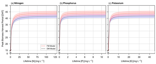
Figure 4.
Peak biomass harvest period, as predicted by SMND µ models for fresh mass and dry mass. Shaded regions represent approximately ±5% of the value of μmax.
As the concentration of each of these three nutrients increases, the peak biomass harvest period rapidly approaches 41.7 days when predicted by dry mass parameters, and 44.0 days when predicted by fresh mass parameters.
3.5. Validation Treatments: Dry and Fresh Mass
Figure 5 presents dry and fresh mass data for the three validation treatments. Parameter values from each model were applied, along with piecewise N, P, and K concentrations via each respective multi-nutrient model.
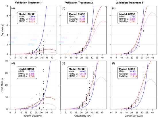
Figure 5.
Integrated dry mass (a–c) and fresh mass (d–f) models for validation treatment 1 (a,d), 2 (b,e), and 3 (c,f). Colored lines represent each respective model. Black dots represent individual dry and fresh mass measurements.
Generally, SMND μ provided the best fit, by wide margins, for estimating dry mass in validation treatments 1 and 2, but was outperformed in validation treatment 3 by the RMND μ model parameters. Meanwhile, SMND μ offered the best fit, by wide margins, for estimating fresh mass in validation treatments 2 and 3, but was outperformed in validation treatment 1 by Monod’s MMN model.
3.6. Biomass Estimation from Wastewater
Figure 6 illustrates the range of estimated dry and fresh biomass cultivated with expected nutrient concentrations found in reclaimed domestic wastewater: 30–60 mg-N L−1, 5–20 mg-P L−1, and 5–40 mg-K L−1 [41,42], with ideal NPK and partially supplemented NPK concentrations provided as a benchmark comparison.
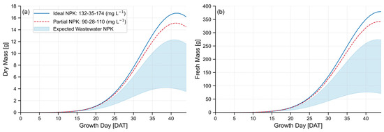
Figure 6.
Expected lettuce growth using reclaimed domestic wastewater based on SMND μ parameters, indicating (a) dry mass, and (b) fresh mass. Lower boundary of shaded wastewater region reflects an NPK of 30-5-5 mg L−1, and upper boundary reflects an NPK of 60-20-40 mg L−1.
This model estimates that reclaimed domestic wastewater can grow Bibb lettuce at approximately 4–12 g dry mass and 75–275 g fresh mass each. Naturally, this falls short of lettuce biomass estimates grown under ideal NPK concentrations, which may reach an average expected peak of 17 g dry mass and 380 g fresh mass. This quantifies wastewater as producing between 20% and 72% of the maximum peak fresh mass when used as the sole source of nutrients.
4. Discussion
4.1. Relative Growth Rates: An Improper Analysis of the Fit to Mass Approach
When using foundational Monod (Figure 1) and Dynamic μ (Figure 2) models optimized for dry mass, the reported RMSE increased substantially from the prior comparable Fit to μ models of the same data [37]. However, such analysis is misleading due to the disconnect between mass and RGR. In short, researchers should optimize for RGR when seeking to model and test RGR, and optimize for biomass when seeking to model and test biomass. The latter is more valid for the majority of practical applications to real-world agricultural solutions.
Despite this mismatch, the Dynamic μ RMSE increased by only ~1 order of magnitude, while Monod’s RMSE increased by >2 orders of magnitude for each nutrient. Meanwhile, Dynamic μ also exhibited lesser shifts in parameter values compared to Monod. Both of these observations can be attributed to Dynamic µ’s improved explanation of the data, providing support for the incorporation of plant maturity’s influence on RGR.
These figures highlight the importance of structuring models correctly towards an intended objective (e.g., predicting growth rate vs. predicting biomass). Understanding this reveals the parallel benefits for researchers who wish to apply this same logic to nutrient uptake via Michaelis-Menten. Rather than optimizing parameters to minimize error in nutrient uptake rate, researchers may choose to minimize error with absolute or cumulative nutrient uptake as measured by nutrient mass. Doing so would give greater weight to uptake by matured plants, which studies have shown to uptake more nutrients, more consistently, but at a slower relative nutrient uptake or flux rate (e.g., U, V, J, or I) than young plants [30,36,44].
4.2. Integrated Dry Mass: A Correct Analysis of the Fit to Mass Approach
Within each treatment subfigure from Figure 3, researchers compare the RMSE of the four models. In this analysis, the SMND μ model frequently exhibits the lowest or near-lowest error. This model performed exceptionally well against all P-limited treatments, good or great in most other treatments, but unusually and comparatively poor in the two lowest N-limited (5 mg-N L−1 and 11 mg-N L−1) treatments. However, these extremely low nitrogen treatments are far below practical application. Furthermore, these two low-nutrient treatments result in exceptionally low and variable biomass. This informs readers that while their relative error may be increased, absolute error remains small.
While the SMND μ model offered the best fit, Monod regularly offered the worst fit (greatest error) of the compared models. The primary distinction that separates Monod from the three Dynamic μ models is the lack of temporal decay. Due to this lack of temporal decay, if additional samples were grown and harvested between 32 and 44 DAT, researchers could track biomass models to gauge accuracy and potential error.
During these 12 days, Monod’s predicted dry mass would increase by 2507% and fresh mass by 2248% due to this exponential growth. Based on the 32 DAT average fresh mass of 250.73 ± 25.41 g, the foundational Monod would predict this Bibb lettuce to reach an average of 5.9 kg (13.0 lbs) each, a target unlikely to be achieved in Bibb lettuce. Lettuce falling short of this lofty prediction would inherently reduce Monod’s predicted μmax, significantly increasing the underestimation of already-underestimated plant mass throughout the majority of the growth period. This would increase Monod’s RMSE even higher than current models, giving it a progressively worse fit as growth periods increase. Meanwhile, SMND μ parameters would estimate the same lettuce to reach a peak average fresh mass of 529 g each, a much more reasonable size expectation for this cultivar of lettuce.
4.3. Integrated Dry Mass: Interpreting Relative Differences
Comparing the single-nutrient Dynamic μ models to the multi-nutrient SMND μ models is complex, representing a change not only in the quantity of nutrients, but also in how the parameters are identified. This comparison can be accomplished using RMND μ, which represents a compilation of single-nutrient model parameters, as the intermediary to compare against.
Using Figure 3, researchers can compare the single-nutrient Dynamic μ to RMND μ biomass models. Because the only difference between these models is the fractional contribution from non-target nutrients, via Equation (5), researchers can expect RMND μ to always be equal to or lower than the Dynamic μ biomass predictions. These two models will be approximately equal only when fractional contributions from non-target nutrients approach 100%, and only under the validity of the RMND μ assumption that all non-target nutrients are non-limiting. Any significant observed differences between Dynamic μ and RMND μ biomass models will indicate increasing limitation from these non-target nutrients, and inherently violate the RMND μ assumption. This sows distrust in the RMND μ model parameters, revealing the model’s shortcomings regardless of improvements or failures in best-fit.
So how does this non-target nutrient limitation compare across treatments? Within N-limited treatments, Figure 3 shows a small amount of additional limitation in the 66 mg-N L−1 and baseline 132 mg-N L−1 treatments. Within the P-limited treatments, there is a significant amount of additional limitation in 2, 5, 12, and baseline 31 mg-P L−1 treatments. And within the K-limited treatments, there is a significant amount of additional limitation across all treatments.
These limitations highlight the importance and value of using a true multi-nutrient model (e.g., SMND μ) over single-nutrient models, including RMND µ. Additionally, it suggests that the methodology would have benefited significantly from either (1) performing more frequent water changes to replenish nutrients, or (2) elevating all non-limiting nutrients in each treatment to above the baseline concentration (e.g., 150% of baseline, instead of 100%). Furthermore, these results may hint that other non-target nutrients (e.g., Mg, S, Ca, Fe, Al, B, Zn, Cu, Mo) may also have unintentionally limited growth. This would be an excellent opportunity for additional research, perhaps solved by one or two additional treatments for each remaining nutrient, using 150% of the baseline for all non-target nutrients.
Now that researchers have identified the shortcomings of the RMND μ model, and by extension, the single-nutrient Dynamic μ model parameters, let us discuss how the SMND μ compares and improves upon the RMND μ biomass models. Primarily, the SMND μ model does not assume non-target nutrients are non-limiting. As such, readers can expect SMND μ to always predict either equal or greater biomass than the RMND μ model output for a given dataset. The distance between these models is indicative of limiting nutrient corrections, inclusive of all target nutrients and treatments, and limited only by the strength of the dataset. This strength is improved with dataset size, a well-executed maximum-growth baseline treatment, and test treatments covering a wide range of permutations of nutrient concentrations.
4.4. Peak Biomass Harvest Date
One feature of the Dynamic μ model is its identification of a peak biomass harvest date, defined as the moment when the ongoing processes of plant decay begin to surpass those fueling plant growth. The date itself may be indicative of the lettuce transitioning from the exponential/log growth phase into the decay phase. The bypassed mention of a stationary phase may result from the improved characterization of growth rate, which blurs the lines between phases as they transition from one to the next [52,53].
This can first be observed in Figure 2, in which the Dynamic μ model can be extrapolated forward along the z-axis beyond 32 DAT and the model crosses the xz-plane in which µ = 0. This breakeven at µ = 0 can be seen as a maximum peak biomass in each of the biomass models (Figure 3, Figure 5, and Figure 6).
Meanwhile, Figure 4 illustrates how this date changes in response to nutrient concentrations. Given the sharp curve seen in Figure 4, nutrient concentration may have little influence on recommended harvest dates, despite its influence on overall biomass. Peak dry biomass occurs on 41.7 DAT, and fresh mass on 44.0 DAT under all except the most extreme nutrient deficiency. With each passing day beyond 44.0 DAT, both plant dry mass and fresh mass will be expected to decrease. While there are potential reasons to harvest prior to this date, there is less justification for harvesting smaller plants after this date.
Near this moment of peak biomass, total dry and fresh biomass changes are minimal and incremental each day, essentially reaching the plateau akin to the stationary growth phase. However, the implication of understanding the characterization of growth rate informs researchers that during the 2.3-day period between 41.7 DAT and 44.0 DAT, Bibb lettuce is losing small amounts of dry mass, but more than compensating for this minor loss with the addition of water weight.
Given that the originating dataset extends only to 32 DAT and decay appears linear up until this date, researchers acknowledge this relationship may become nonlinear beyond 32 DAT. Additional data of lettuce grown well beyond 32 DAT (e.g., 45–65 DAT) would be required to support or refute both the linear or nonlinear nature, as well as support or refute peak biomass harvest dates.
4.5. Biomass Model Validation
These three validation treatments seen in Figure 5 provide promising support for the SMND μ model. As anticipated, this model exhibited the lowest error across both dry mass and fresh mass observations in nearly all treatments, failing to provide the best fit in two of the six analyses. On average, SMND μ exhibited 52.5% less error than MMN and 25.8% less error than RMND μ models across these three validation treatments.
The two exceptions to this are validation treatment 3 (VT3) for estimating dry mass, and validation treatment 1 (VT1) for estimating fresh mass. These instances were each outcompeted by a different model: RMND μ for dry mass in VT3, and MMN for fresh mass in VT1. Furthermore, the amount by which they were outcompeted in these two treatments was relatively low.
This validation shows strong support for the use of the SMND μ model to derive and apply parameters for estimating biomass growth. Of course, additional validation treatments, using a higher quantity of more variable NPK concentrations, would remain helpful for validation.
4.6. Biomass Estimation from Wastewater
Figure 6 illustrates both the dry and fresh mass of lettuce grown using domestic wastewater. Even the upper range of wastewater, with the most optimistic NPK nutrient concentrations, is predicted to grow lettuce with significantly less dry and fresh biomass, peaking at ~72% of fresh biomass grown under ideal nutrient concentrations.
Beyond biomass differences attributed to nutrient concentrations, readers will also notice the large difference in biomass as plants grow from 32 DAT to 44 DAT, supporting that the experiments on which these models were based were harvested prematurely. While some studies recommend early harvest periods for similar cultivars of lettuce between 28 and 35 DAT [13,54,55,56], many others support harvest periods of 40–50 DAT [14,16,57,58], which may be a more practical growth period for farmers and one which will provide improved data for agricultural researchers.
4.7. Applying Models to Estimate Profit
Researchers, farmers, and engineers can also use this framework to estimate potential profits and guide decisions, such as how much of each nutrient to supplement. One simplified example is presented in Equations (10)–(12). Equation (10) calculates the marginal cost to supplement each nutrient i by taking the difference between the measured wastewater nutrient concentration and its desired target nutrient concentration . This difference is multiplied by the total system volume VR, cost per unit of nutrient i, and optionally multiplied by the depletion rate DR for nutrient i and estimated time until harvest. This optional component may not be needed for large systems, but small systems which see large swings in nutrient concentrations will require this extra step to estimate the costs of maintaining elevated concentrations.
Equation (11) calculates the marginal revenue to bring the expected fresh mass from wastewater () up to the expected fresh mass grown at the desired target nutrient concentration () for a given quantity of plants. Finally, Equation (12) calculates expected profits as the difference between marginal revenue and marginal costs. Due to marginal revenue decreasing over time as plants approach peak biomass, it is expected to be more profitable to err on harvesting slightly early rather than harvesting comparably late.
Of course, this example represents a simplified analysis. Multiple other nutrients can be considered beyond NPK. Furthermore, nutrient costs can be combined; for example, potassium nitrate (KNO3) can be supplemented to combine and reduce the costs of both potassium and nitrogen. Meanwhile, other methods outside supplementation (e.g., wastewater processing, concentration) would entail alternative calculations for marginal costs, but influence a large number of nutrients simultaneously. Regardless, this model provides the framework and parameters to similarly estimate resulting profits from modifications to nutrient supply.
4.8. Model Limitations and Practical Applications
At this point, it is of the utmost importance to remind readers that these parameters and results are based on specific environmental variables. While this type of research and identified parameters are inherently linked to these specific environmental variables, these models can be integrated into larger mechanistic models in order to factor in the expected influence of other environmental variables. Furthermore, additional research can apply these findings, with or without larger mechanistic model components, to investigate the nutrient uptake and biomass growth of other nutrients and/or plants.
However, an unaccounted-for environmental influence is the style of hydroponic system, for which this study used a vertical NFT (nutrient film technique) farm-wall style of hydroponics. This may influence the lettuce to grow internal structures to counteract the perpendicular force of gravity, contrary to conventional agriculture and common hydroponic systems such as deep water culture. Unfortunately, more research is needed to understand and identify if such effects occur and their significance.
Furthermore, the practical application of these models extends beyond simply recovering nutrients from wastewater. By recovering nutrients from domestic wastewater for application to agriculture, these models play a crucial role in the development of a circular economy. In this, nutrients can be recycled indefinitely (yet not necessarily infinitely), vastly extending the utility of nutrients from single-use disposable resources into reusable resources. This has the added benefit of reducing many monetary costs and harmful environmental impacts associated with fertilizer production [59,60,61,62] and wastewater management [43,63,64,65]. Meanwhile, the Organic Processor Assembly, which recycles wastewater effluent to grow pak choi vegetables, represents a current practical application of a circular economy for which agricultural models can apply [66].
These circular economies are applicable both at a large civilization-scale and at a small community-scale. These smaller community-scale implementations support decentralization, reducing transportation costs and inefficiencies while also reducing agricultural dependency on distant and volatile food-supply systems [67,68]. Such applications extend to serve local communities, isolated research posts, space stations, and large ships at sea (e.g., cargo ships, cruises, aircraft carriers and military vessels, etc.).
4.9. Future Research Recommendations
The first recommendation for future research would be to replicate this methodology using plants receiving 150% of ideal nutrients in order to refine or confirm that μmax and other parameters were not hindered by limited non-target nutrients. These will directly address and mitigate sub-maximal growth caused by plants’ rapid and immediate uptake of nutrients.
Furthermore, research plans can extend the growth period to beyond 49 DAT, while harvest dates for this new treatment could be modified from {14, 18, 21, 25, 28, and 32} DAT to {14, 21, 28, 35, 42, 49, 56, and 63} DAT. The longer growth period can identify if the decreasing RGR remains linear over the extended period and reveal if RGR decreases at a decreasing rate beyond 32 DAT, approaching an asymptote above zero rather than crossing into decay [30,33,34,35,36]. This would thus support or refute the validity of the identified peak fresh biomass on 44 DAT.
Another simple but more intensive follow-up study could perform a similar analysis for Mg, S, Ca, and Fe, potentially utilizing 4% and 15% treatments for each nutrient. This would gather kinetic parameters for lesser-studied macronutrients and identify if the passive uptake of calcium via the transpiration stream [27,69] causes significant model deviation.
The results of this study are empirical in nature, and as such, they identify and characterize relationships. In doing so, they add significant value in practical application and predictive capabilities. However, they do not explain causal mechanisms for maturity-based decay. Some studies have speculated this is attributed to self-shading [15,70,71,72], but these speculations are thus far unsubstantiated. Furthermore, this Dynamic μ model considers this decay to be linear. Additional research can explore this relationship from a mechanistic perspective, gathering support for causal mechanisms while refining the relationship with a more accurate characterization that is supported by physical, chemical, and/or biological principles.
If closed-loop hydroponics are used indefinitely, one concern for farmers is the accumulation of unused nutrients. These excess nutrients could eventually accumulate into toxic concentrations, resulting in growth inhibition. An additional research initiative could perform experiments with >1000% of individually targeted baseline nutrient concentrations for nutrients of concern. This data could be used to identify growth inhibition parameters, such as those of Haldane [9,10]. And whereas macronutrients represent the primary focus of growth kinetics, inhibition kinetics may be equally concerned with both macronutrients and micronutrients. This may be beneficial for sustainable long-term use of hydroponic systems which choose not to discard or flush nutrient solutions, and thus are expected to see lesser-utilized nutrients at elevated concentrations after many consecutive crop seasons.
Finally, modeling efforts can apply the influence of plant age, via Dynamic μ, to improve predictive capabilities of nutrient uptake, modifying Michaelis-Menten to characterize absolute or cumulative nutrient uptake. It can incorporate nutrient concentration minimums Smin [8]. Updated models can analyze profitability for using agriculture to remove nutrients from wastewater, taking a wastewater treatment perspective.
5. Conclusions
This study develops the first agricultural (fresh and dry) biomass models which consider the influence of plant maturity on RGR, incorporating multiple limiting nutrients, and adapting models to accommodate a variable nutrient supply. Analysis of models, validation treatments, and comparison to alternative models show strong support for the SMND μ model and identified parameters. Meanwhile, observations in shortcomings of its own data source indicate room for improvement for future research.
Furthermore, this study explores practical applications of agricultural modeling for nutrient recovery from wastewater. It quantifies the range of expected biomass based on upper and lower boundaries for N, P, and K concentrations in reclaimed domestic wastewater. It identifies the peak biomass harvest date as a function of nutrient concentration, and exemplifies how to apply these models to estimate the profitability of supplemental nutrients, laying a strong foundation for the integration of wastewater nutrient recovery and agricultural production.
Supplementary Materials
The following supporting information can be downloaded at https://www.mdpi.com/article/10.3390/agriculture15181927/s1, Figure S1: Integrated Fresh Mass Model Comparison.
Author Contributions
Conceptualization, A.S. and Y.C.; methodology, A.S. and A.A.; software, A.S., A.A. and Y.S.; validation, A.S. and A.A.; formal analysis, A.S. and A.A.; investigation, A.S. and A.A.; resources, Y.C.; data curation, A.S.; writing—original draft preparation, A.S. and A.A.; writing—review and editing, A.S., A.A., Y.S. and Y.C.; visualization, A.S., A.A. and Y.S.; supervision, A.S. and Y.C.; project administration, A.S. and Y.C.; funding acquisition, Y.C. All authors have read and agreed to the published version of the manuscript.
Funding
This research was supported by the U.S. Department of Agriculture’s National Institute of Food and Agriculture (Award Nos. 2018-68011-28371, 2021-67021-34499, 2024-67021-41534, and 2024-67021-42876), National Science foundation (Award Nos. 2419122 and 2112533), and a seed grant from the Brook Byers Institute for Sustainable Systems (BBISS).
Institutional Review Board Statement
Not applicable.
Data Availability Statement
The original data presented in the study are openly available in the USDA’s Ag Data Commons data repositories: “Dataset for the Hydroponic Cultivation of Bibb Lettuce in NPK-Limited Conditions”, DOI: https://doi.org/10.15482/USDA.ADC/28801286.v1, accessed on 22 August 2025; “Validation Dataset for Hydroponically Cultivated Bibb Lettuce”, DOI: https://doi.org/10.15482/USDA.ADC/29646779, accessed on 22 August 2025; and on figshare: “Python Script for Modeling Hydroponically Cultivated Bibb Lettuce”, DOI: https://doi.org/10.6084/m9.figshare.29897459, accessed on 22 August 2025.
Acknowledgments
We also wish to offer a special thank you to the many student researchers who, between classes, helped maintain hydroponic operations between 2018 and 2024. Their collective contribution made this research possible, including during the COVID-19 pandemic. They are as follows (*indicates exceptional contribution): Monica Lester, Wiley Helm, Jasmin Lopez, Mengquiao Gao, Dylan Lambeth, Teresa (Rose) Mckenna, Jazmin Lucio, Matthew (Tom) Ennis, Teagan Groh*, Fabin Saju, Camille Butkus, Bethel Mamo, Talia Zheng, Nok Sam Leong, Caroline Krall, Corinna Alting, Maya Kahn*, Lily Luong, Henry (Elijah) Craig, Rachel Nichols, Emma Carmical*, Ian Moss, Catherine Rekos, Pauline Yakubovich, Andrea Green, Abigail Crombie, Cambria Caliendo, Luisa Bricker, Annasaria Antaran, William Skillen, Joshua Guthrie*, Amanosi Maiki, Olivia Edwards, Evan Beckley, Olivia Felker, Hridee Haq, Alina Sullivan, Jieon Kim, Terry Kim, Catelyn Chamblee, Aidan Blackshire, and Eric Anderson.
Conflicts of Interest
The authors declare no conflicts of interest. The funders had no role in the design of the study, in the collection, analyses, or interpretation of data, in the writing of the manuscript, or in the decision to publish the results.
References
- Michaelis, L.; Menten, M.L. Die kinetik der invertinwirkung. Biochem. Z. 1913, 49, 333–369. [Google Scholar] [CrossRef]
- Johnson, K.A.; Goody, R.S. The original Michaelis constant: Translation of the 1913 Michaelis-Menten paper. Biochemistry 2011, 50, 8264–8269. [Google Scholar] [CrossRef]
- Hsu, S.B.; Hubbell, S.; Waltman, P. A mathematical theory for single-nutrient competition in continuous cultures of micro-organisms. SIAM J. Appl. Math. 1977, 32, 366–383. [Google Scholar] [CrossRef]
- Button, D.K. Kinetics of nutrient-limited transport and microbial growth. Microbiol. Rev. 1985, 49, 270–297. [Google Scholar] [CrossRef] [PubMed]
- Monod, J. The growth of bacterial cultures. Annu. Rev. Microbiol. 1949, 3, 371–394. [Google Scholar] [CrossRef]
- Zinn, M.; Witholt, B.; Egli, T. Dual nutrient limited growth: Models, experimental observations, and applications. J. Biotechnol. 2004, 113, 263–279. [Google Scholar] [CrossRef] [PubMed]
- Bader, F.G. Analysis of double-substrate limited growth. Biotechnol. Bioeng. 1978, 20, 183–202. [Google Scholar] [CrossRef] [PubMed]
- Rittmann, B.E.; Mccarty, P.L. Model of steady-state-biofilm kinetics. Biotechnol. Bioeng. 1980, 22, 2343–2357. [Google Scholar] [CrossRef]
- Briggs, G.E.; Haldane, J.B.S. A note on the kinetics of enzyme action. Bot. Biochem. Lab. 1925, 19, 338. [Google Scholar] [CrossRef] [PubMed]
- Andrew, J.F. Dynamic model of the anaerobic digestion process. J. Sanit. Eng. Div. 1969, 95, 95–116. [Google Scholar] [CrossRef]
- Kaiser, G. Microbiology; LibreTexts: Cantonsville, MD, USA, 2025. [Google Scholar]
- Steil, A. Vegetable Harvest Guide. Available online: https://yardandgarden.extension.iastate.edu/how-to/vegetable-harvest-guide (accessed on 5 June 2025).
- Brechner, M.; Both, A.J. Hydroponic lettuce handbook. Cornell Control. Environ. Agric. 1996, 834, 504–509. [Google Scholar]
- Both, A.J.; Albright, L.D.; Langhans, R.W.; Reiser, R.A.; Vinzant, B.G. Hydroponic lettuce production influenced by integrated supplemental light levels in a controlled environment agriculture facility: Experimental results. Acta Hortic. 1994, 418, 45–52. [Google Scholar] [CrossRef]
- Tei, F.; Scaife, A.; Aikman, D.P. Growth of lettuce, onion, and red beet. 1. Growth analysis, light interception, and radiation use efficiency. Ann. Bot. 1996, 78, 633–643. [Google Scholar] [CrossRef]
- Gavhane, K.P.; Hasan, M.; Singh, D.K.; Kumar, S.N.; Sahoo, R.N.; Alam, W. Determination of optimal daily light integral (DLI) for indoor cultivation of iceberg lettuce in an indigenous vertical hydroponic system. Sci. Rep. 2023, 13, 10923. [Google Scholar] [CrossRef] [PubMed]
- Ellis, J.L.; Jacobs, M.; Dijkstra, J.; van Laar, H.; Cant, J.P.; Tulpan, D.; Ferguson, N. Review: Synergy between mechanistic modelling and data-driven models for modern animal production systems in the era of big data. Animal 2020, 14, s223–s237. [Google Scholar] [CrossRef]
- Seginer, I.; Buwalda, F.; van Straten, G. Nitrate concentration in greenhouse lettuce: A modeling study. Acta Hortic. 1998, 456, 189–197. [Google Scholar] [CrossRef]
- Keating, B.A.; Carberry, P.S.; Hammer, G.L.; Probert, M.E.; Robertson, M.J.; Holzworth, D.; Huth, N.I.; Hargreaves, J.N.G.; Meinke, H.; Hochman, Z.; et al. An overview of APSIM, a model designed for farming systems simulation. Eur. J. Agron. 2003, 18, 267–288. [Google Scholar] [CrossRef]
- Van Evert, F.K.; Campbell, G.S. CropSyst: A collection of object-oriented simulation models of agricultural systems. Agron. J. 1994, 86, 325–331. [Google Scholar] [CrossRef]
- Baker, R.E.; Peña, J.M.; Jayamohan, J.; Jérusalem, A. Mechanistic models versus machine learning, a fight worth fighting for the biological community? Biol. Lett. 2018, 14, 20170660. [Google Scholar] [CrossRef]
- Dream, R. Mechanistic modeling: Biotechnology manufacturing. Am. Pharm. Rev. 2025, 28, 26–37. [Google Scholar]
- Gherman, I.M.; Abdallah, Z.S.; Pang, W.; Gorochowski, T.E.; Grierson, C.S.; Marucci, L. Bridging the gap between mechanistic biological models and machine learning surrogates. PLoS Comput. Biol. 2023, 19, e1010988. [Google Scholar] [CrossRef]
- Mathieu, J.; Linker, R.; Levine, L.; Albright, L.; Both, A.J.; Spanswick, R.; Wheeler, R.; Wheeler, E.; DeVilliers, D.; Langhans, R. Evaluation of the NICOLET model for simulation of short-term hydroponic lettuce growth and nitrate uptake. Biosyst. Eng. 2006, 95, 323–337. [Google Scholar] [CrossRef]
- Ioslovich, I.; Seginer, I.; Baskin, A. Fitting the nicolet lettuce growth model to plant-spacing experimental data. Biosyst. Eng. 2002, 83, 361–371. [Google Scholar] [CrossRef]
- Juárez-Maldonado, A.; De-Alba-Romenus, K.; Ramírez-Sosa, M.I.M.; Benavides-Mendoza, A.; Robledo-Torres, V. An experimental validation of NICOLET B3 mathematical model for lettuce growth in the southeast region of Coahuila Mexico by dynamic simulation. In Proceedings of the 2010 7th International Conference on Electrical Engineering Computing Science and Automatic Control, Tuxtla Gutierrez, Mexico, 8–10 September 2010; pp. 128–133. [Google Scholar] [CrossRef]
- Silberbush, M.; Ben-Asher, J.; Ephrath, J.E. A model for nutrient and water flow and their uptake by plants grown in a soilless culture. Plant Soil 2005, 271, 309–319. [Google Scholar] [CrossRef]
- Rengel, Z. Mechanistic simulation models of nutrient uptake: A review. Plant Soil 1993, 152, 161–173. [Google Scholar] [CrossRef]
- Swiader, J.M.; Freiji, F.G. Characterizing nitrate uptake in lettuce using very-sensitive ion chromatography. J. Plant Nutr. 1996, 19, 15–27. [Google Scholar] [CrossRef]
- Steingrobe, B.; Schenk, M.K. Simulation of the maximum nitrate inflow (Imax) of lettuce (Lactuca sativa L.) grown under fluctuating climatic conditions in the greenhouse. Plant Soil 1993, 155–156, 163–166. [Google Scholar] [CrossRef]
- Wang, B.; Shen, Q. Effects of ammonium on the root architecture and nitrate uptake kinetics of two typical lettuce genotypes grown in hydroponic systems. J. Plant Nutr. 2012, 35, 1497–1508. [Google Scholar] [CrossRef]
- Zhang, K.; Burns, I.G.; Turner, M.K. Derivation of a dynamic model of the kinetics of nitrogen uptake throughout the growth of lettuce: Calibration and validation. J. Plant Nutr. 2008, 31, 1440–1460. [Google Scholar] [CrossRef]
- Pommerening, A.; Muszta, A. Methods of modelling relative growth rate. For. Ecosyst. 2015, 2, 5. [Google Scholar] [CrossRef]
- Holsteijn Van, H.M.C. Growth of Lettuce II: Quantitative Analysis of Growth; Veenman: Wageningen, The Netherlands, 1980; pp. 1–24. [Google Scholar]
- Albornoz, F.; Lieth, J.H. Daily macronutrient uptake patterns in relation to plant age in hydroponic lettuce. J. Plant Nutr. 2016, 39, 1357–1364. [Google Scholar] [CrossRef]
- Edwards, J.H.; Barber, S.A. Nitrogen uptake characteristics of corn roots at low N concentration as influenced by plant age 1. Agron. J. 1976, 68, 17–19. [Google Scholar] [CrossRef]
- Sharkey, A.; Altman, A.; Sun, Y.; Igou, T.K.S.; Chen, Y. Characterizing the temporally dynamic nature of relative growth rates: A kinetic analysis on nitrogen-, phosphorus-, and potassium-limited growth. Agriculture 2025, 15, 1641. [Google Scholar] [CrossRef]
- Mattson, N.S.; Peters, C. A recipe for hydroponic success. Insid. Grow. 2014, 2014, 16–19. [Google Scholar]
- Uchida, R.; Silva, J.A. Essential nutrients for plant growth: Nutrient functions and deficiency symptoms. In Plant Nutrient Management in Hawaii’s Soils, Approaches for Tropical and Subtropical Agriculture; College of Tropical Agriculture and Human Resources: Honolulu, HI, USA, 2000; pp. 31–55. ISBN 978-1-929325-08-5. [Google Scholar]
- Sambo, P.; Nicoletto, C.; Giro, A.; Pii, Y.; Valentinuzzi, F.; Mimmo, T.; Lugli, P.; Orzes, G.; Mazzetto, F.; Astolfi, S.; et al. Hydroponic solutions for soilless production systems: Issues and opportunities in a smart agriculture perspective. Front. Plant Sci. 2019, 10, 923. [Google Scholar] [CrossRef]
- Li, W.-W.; Yu, H.; Rittmann, B.E. Reuse water pollutants. Nature 2015, 528, 29–31. [Google Scholar] [CrossRef]
- Chojnacka, K.; Witek-Krowiak, A.; Moustakas, K.; Skrzypczak, D.; Mikula, K.; Loizidou, M. A transition from conventional irrigation to fertigation with reclaimed wastewater: Prospects and challenges. Renew. Sustain. Energy Rev. 2020, 130, 109959. [Google Scholar] [CrossRef]
- Saliu, T.D.; Oladoja, N.A. Nutrient recovery from wastewater and reuse in agriculture: A review. Environ. Chem. Lett. 2021, 19, 2299–2316. [Google Scholar] [CrossRef]
- Sharkey, A.; Altman, A.; Cohen, A.R.; Groh, T.; Igou, T.K.S.; Ferrarezi, R.S.; Chen, Y. Modeling Bibb lettuce nitrogen uptake and biomass productivity in vertical hydroponic agriculture. Agriculture 2024, 14, 1358. [Google Scholar] [CrossRef]
- Modarelli, G.C.; Paradiso, R.; Arena, C.; De Pascale, S.; Van Labeke, M.C. High light intensity from blue-red LEDs enhance photosynthetic performance, plant growth, and optical properties of red lettuce in controlled environment. Horticulturae 2022, 8, 114. [Google Scholar] [CrossRef]
- Virtanen, P.; Gommers, R.; Oliphant, T.E.; Haberland, M.; Reddy, T.; Cournapeau, D.; Burovski, E.; Peterson, P.; Weckesser, W.; Bright, J.; et al. SciPy 1.0: Fundamental algorithms for scientific computing in Python. Nat. Methods 2020, 17, 261–272. [Google Scholar] [CrossRef]
- Muloiwa, M.; Nyende-Byakika, S.; Dinka, M. Comparison of unstructured kinetic bacterial growth models. S. Afr. J. Chem. Eng. 2020, 33, 141–150. [Google Scholar] [CrossRef]
- Teissier, G. Growth of bacterial populations and the available substrate concentration. Rev. Sci. Instrum. 1942, 3208, 209–214. [Google Scholar]
- Richards, F.J. A flexible growth function for empirical use. J. Exp. Bot. 1959, 10, 290–301. [Google Scholar] [CrossRef]
- Gompertz, B. Expressive of the law of human mortality and on a new mode of determining the value of life contingencies. Philos. Trans. R. Soc. 1825, 115, 513–585. [Google Scholar] [CrossRef]
- Zeide, B. Analysis of growth equations. For. Sci. 1993, 39, 594–616. [Google Scholar] [CrossRef]
- Madigan, M.T.; Martinko, J.M.; Bender, K.S.; Buckley, D.H.; Stahl, D.A. Brock Biology of Micro-Organisms, 14th ed.; Pearson: London, UK, 1992; ISBN 9780321897398. [Google Scholar]
- Pepper, I.L.; Gerba, C.P.; Gentry, T.J. Environmental Microbiology, 3rd ed.; Wiley: Hoboken, NJ, USA, 2014; ISBN 9780123946263. [Google Scholar]
- Hydroponic Lettuce: What to Know. Available online: https://risegardens.com/blogs/communitygarden/hydroponic-lettuce-what-to-know-s25 (accessed on 1 July 2025).
- Jung, D.H.; Kim, D.; Yoon, H.I.; Moon, T.W.; Park, K.S.; Son, J.E. Modeling the canopy photosynthetic rate of romaine lettuce (Lactuca sativa L.) grown in a plant factory at varying CO2 concentrations and growth stages. Hortic. Environ. Biotechnol. 2016, 57, 487–492. [Google Scholar] [CrossRef]
- Martínez-Moreno, A.; Carmona, J.; Martínez, V.; Garcia-Sánchez, F.; Mestre, T.C.; Navarro-Pérez, V.; Cámara-Zapata, J.M. Reducing nitrate accumulation through the management of nutrient solution in a floating system lettuce (Lactuca sativa L.). Sci. Hortic. 2024, 336, 113377. [Google Scholar] [CrossRef]
- Hasan, M.R.; Tahsin, A.K.M.M.; Islam, M.N.; Ali, M.A.; Uddain, J. Growth and yield of lettuce (Lactuca sativa L.) influenced as nitrogen fertilizer and plant spacing. IOSR J. Agric. Vet. Sci. 2017, 10, 62–71. [Google Scholar] [CrossRef]
- Lee, A.C.; Liao, F.S.; Lo, H.F. Temperature, daylength, and cultivar interact to affect the growth and yield of lettuce grown in high tunnels in subtropical regions. HortScience 2015, 50, 1412–1418. [Google Scholar] [CrossRef]
- Steen, I.; Agro, K. Phosphorus availability in the 21st century—Management of a non-renewable resource. Phosphorus Potassium 1998, 217, 25–31. [Google Scholar]
- Snyder, C.S.; Bruulsema, T.W.; Jensen, T.L.; Fixen, P.E. Review of greenhouse gas emissions from crop production systems and fertilizer management effects. Agric. Ecosyst. Environ. 2009, 133, 247–266. [Google Scholar] [CrossRef]
- Gellings, C.W.; Parmenter, K.E. Energy efficiency in fertilizer production and use. Effic. Use Conserv. Energy 2016, 2, 123–136. [Google Scholar]
- Batstone, D.J.; Hülsen, T.; Mehta, C.M.; Keller, J. Platforms for energy and nutrient recovery from domestic wastewater: A review. Chemosphere 2015, 140, 2–11. [Google Scholar] [CrossRef] [PubMed]
- Beman, J.M.; Arrigo, K.R.; Matson, P.A. Agricultural runoff fuels large phytoplankton blooms in vulnerable areas of the ocean. Nature 2005, 434, 211–214. [Google Scholar] [CrossRef]
- Akinnawo, S.O. Eutrophication: Causes, consequences, physical, chemical and biological techniques for mitigation strategies. Environ. Chall. 2023, 12, 100733. [Google Scholar] [CrossRef]
- Smith, V.H.; Schindler, D.W. Eutrophication science: Where do we go from here? Trends Ecol. Evol. 2009, 24, 201–207. [Google Scholar] [CrossRef]
- Smith, A.; Bullard, T.; Saetta, D.; Haarmann, K.; Akepeu, N.; Yeh, D.; Fischer, J.; Roberson, L. Using effluent from a hybrid anaerobic membrane bioreactor treating fecal waste for hydroponic fertigation of pak choi. In Proceedings of the 2023 International Conference on Environmental Systems, Calgary, AB, Canada, 16–20 July 2023. [Google Scholar]
- Enriquez, J.P. Food self-sufficiency: Opportunities and challenges for the current food system. Biomed. J. Sci. Tech. Res. 2020, 31, 23984–23989. [Google Scholar] [CrossRef]
- Van Ginkel, S.W.; Igou, T.; Chen, Y. Energy, water and nutrient impacts of California-grown vegetables compared to controlled environmental agriculture systems in Atlanta, GA. Resour. Conserv. Recycl. 2017, 122, 319–325. [Google Scholar] [CrossRef]
- Silberbush, M.; Ben-Asher, J. Simulation study of nutrient uptake by plants from soilless cultures as affected by salinity buildup and transpiration. Plant Soil 2001, 233, 59–69. [Google Scholar] [CrossRef]
- Scaife, M.A.A. The early relative growth rates of six lettuce cultivars as affected by temperature. Ann. Appl. Biol. 1973, 74, 119–128. [Google Scholar] [CrossRef]
- Paine, C.E.T.; Marthews, T.R.; Vogt, D.R.; Purves, D.; Rees, M.; Hector, A.; Turnbull, L.A. How to fit nonlinear plant growth models and calculate growth rates: An update for ecologists. Methods Ecol. Evol. 2012, 3, 245–256. [Google Scholar] [CrossRef]
- Burns, I.G.; Broadley, M.R.; Seginer, I.; Burns, A.; Escobar-gutie, A.J.; White, P.J. The nitrogen and nitrate economy of butterhead lettuce (Lactuca sativa var. capitata L.). J. Exp. Bot. 2003, 54, 2081–2090. [Google Scholar] [CrossRef] [PubMed]
Disclaimer/Publisher’s Note: The statements, opinions and data contained in all publications are solely those of the individual author(s) and contributor(s) and not of MDPI and/or the editor(s). MDPI and/or the editor(s) disclaim responsibility for any injury to people or property resulting from any ideas, methods, instructions or products referred to in the content. |
© 2025 by the authors. Licensee MDPI, Basel, Switzerland. This article is an open access article distributed under the terms and conditions of the Creative Commons Attribution (CC BY) license (https://creativecommons.org/licenses/by/4.0/).