Neural Network-Based SLAM/GNSS Fusion Localization Algorithm for Agricultural Robots in Orchard GNSS-Degraded or Denied Environments

Abstract

To address the issue of agricultural robot loss of control caused by GNSS signal degradation or loss in complex agricultural environments such as farmland and orchards, this study proposes a neural network-based SLAM/GNSS fusion localization algorithm aiming to enhance the robot’s localization accuracy and stability in weak or GNSS-denied environments. It achieves multi-sensor observed pose coordinate system unification through coordinate system alignment preprocessing, optimizes SLAM poses via outlier filtering and drift correction, and dynamically adjusts the weights of poses from distinct coordinate systems via a neural network according to the GDOP. Experimental results on the robotic platform demonstrate that, compared to the SLAM algorithm without pose optimization, the proposed SLAM/GNSS fusion localization algorithm reduced the whole process average position deviation by 37%. Compared to the fixed-weight fusion localization algorithm, the proposed SLAM/GNSS fusion localization algorithm achieved a 74% reduction in average position deviation during transitional segments with GNSS signal degradation or recovery. These results validate the superior positioning accuracy and stability of the proposed SLAM/GNSS fusion localization algorithm in weak or GNSS-denied environments. Orchard experimental results demonstrate that, at an average speed of 0.55 m/s, the proposed SLAM/GNSS fusion localization algorithm achieves an overall average position deviation of 0.12 m, with average position deviation of 0.06 m in high GNSS signal quality zones, 0.11 m in transitional sections under signal degradation or recovery, and 0.14 m in fully GNSS-denied environments. These results validate that the proposed SLAM/GNSS fusion localization algorithm maintains high localization accuracy and stability even under conditions of low and highly fluctuating GNSS signal quality, meeting the operational requirements of most agricultural robots.

1. Introduction

In recent years, China has faced intensifying population ageing, with rural labor shortages emerging as a critical constraint on rural revitalization. Agricultural automation and intelligentization represent an irreversible trend for the future of farming [1,2,3]. With continuous advancements in technology, agricultural robots have emerged as a viable solution to replace human labor in repetitive agricultural tasks. These robots not only significantly enhance operational efficiency and quality but also inject new momentum into sustainable agricultural development. Their immense potential and promising prospects have garnered significant attention within the global agriculture technology sector [4,5,6]. Among the core technologies for agricultural robots, positioning systems play a pivotal role, serving as the fundamental enabler for autonomous navigation operations [7,8,9].

In open-field environments, RTK (Real-Time Kinematic)-enabled GNSSs (Global Navigation Satellite Systems) provide centimeter-level positioning accuracy, which has become the primary technical dependency for current agricultural robot navigation systems [10,11,12,13,14,15]. These works collectively demonstrate the critical role of high-precision GNSSs in enabling key functionalities such as autonomous navigation of agricultural vehicles, precise path management, and trajectory tracking. However, in occluded environments, GNSS signals suffer from degradation or even loss of fixed solutions, leading to drastic declines in positioning accuracy that severely compromise the reliability of autonomous navigation. Lidar (Light Detection and Ranging) systems, whether 2D or 3D configurations, provide autonomous machines with comprehensive environmental perception capabilities through active laser scanning. This environmental awareness compensates for GNSS limitations by enabling real-time ego-motion estimation during signal outages, thereby enhancing operational safety in agricultural scenarios. Given the critical need for reliable positioning in weak or GNSS-denied environments, achieving continuous and precise robot localization has emerged as a key research focus in agricultural robotics [16,17,18,19,20,21,22]. Cao et al. [23] proposed a neural network-based predictive MEMS-SINS error feedback correction method. This approach trains the neural network during GPS (Global Positioning System) availability and utilizes the trained model to predict MEMS-SINS errors during GPS outages. In four 50 s simulated GPS-denied experiments, the method achieved an average position error of 3.8 m. Shen et al. [24] proposed a Radial Basis Function-based Multilayer Perceptron-assisted Cubature Kalman Filter to compensate for position and velocity errors during GPS outages. In a 500 s GPS signal interruption test, the algorithm’s mean square error was below 23.11 m. Liu et al. [25] addressed the challenge of cumulative errors in MEMS-INS during GPS signal loss by developing a neural network-aided GPS/MEMS-INS integrated navigation system. Experimental simulations under GPS-denied conditions demonstrated that this approach outperformed traditional frameworks using a Standard Kalman Filter and Unscented Kalman Filter, achieving approximately 65% improvement in velocity and positional accuracy. Zhang et al. [26] proposed a BDS (BeiDou Navigation Satellite System) outage endurance method for agricultural machinery navigation. By designing a Self-Calibrating Variable-Structure Kalman Filter for BDS/INS data fusion, this approach maintains straight-line tracking accuracy within limited durations. In robotic platform trials, during 20 s simulated BDS outages, the method achieved an average lateral deviation of 0.31 m on linear paths and an average positioning discrepancy of 0.77 m between the INS (Inertial Navigation System) and BDS on rectangular paths. However, cumulative errors inherent to the INS system limit its long-term operational viability. Wei et al. [27] addressed the challenge of GNSS signal occlusion in orchard environments by implementing a Kalman Filter-based fusion framework integrating GNSS and LiDAR data. To mitigate motion-induced distortion in LiDAR scans, an odometry-aided correction method was applied, enabling autonomous navigation for agricultural robots. Experimental results demonstrated a mean lateral deviation of less than 11 cm between actual and planned trajectories. However, the validity of GNSS signal availability during trials remains unverified, as the experiments did not isolate GNSS signals to quantify environmental signal degradation levels. Hu et al. [28] proposed a laser-based localization method for agricultural robots, which achieves robot positioning by fusing ToF (time-of-flight) measurements from laser scanning with point cloud features acquired by a LiDAR receiver. Experimental results demonstrated that the average maximum deviations during straight-line and curvilinear motion were 4.1 cm and 6.2 cm, respectively. This method is primarily applicable to GNSS-denied indoor environments such as hangars and greenhouses, requiring unobstructed visibility between the LiDAR and receiver. However, its effectiveness is limited in outdoor scenarios due to potential occlusions. The aforementioned research studies provide valuable insights into achieving continuous and precise robot localization in weak or GNSS-denied environments. However, they still face limitations such as relatively low localization accuracy and suboptimal stability, which may cause trajectory deviations during autonomous navigation, operational failures in precision farming tasks, and potential safety hazards in complex agricultural environments.

To address the aforementioned issues, this study proposes a neural network-based SLAM/GNSS fusion localization algorithm. The algorithm integrates the local accuracy of LiDAR-inertial odometry with the global stability of a GNSS. It achieves multi-sensor observed pose coordinate system unification through coordinate system alignment preprocessing, optimizes SLAM (Simultaneous Localization and Mapping) poses via outlier filtering and drift correction, and dynamically adjusts the weights of poses from distinct coordinate systems via a neural network according to the GDOP (Geometric Dilution of Precision). These mechanisms collectively enhance the robot’s localization accuracy and stability in weak or GNSS-denied environments. A wheeled differential-drive robotic platform was developed to preliminarily validate the algorithm’s performance. Furthermore, field experiments were conducted in actual orchard environments to investigate the algorithm’s effectiveness under orchard terrain conditions and tree-obstructed scenarios.

2. Materials and Methods

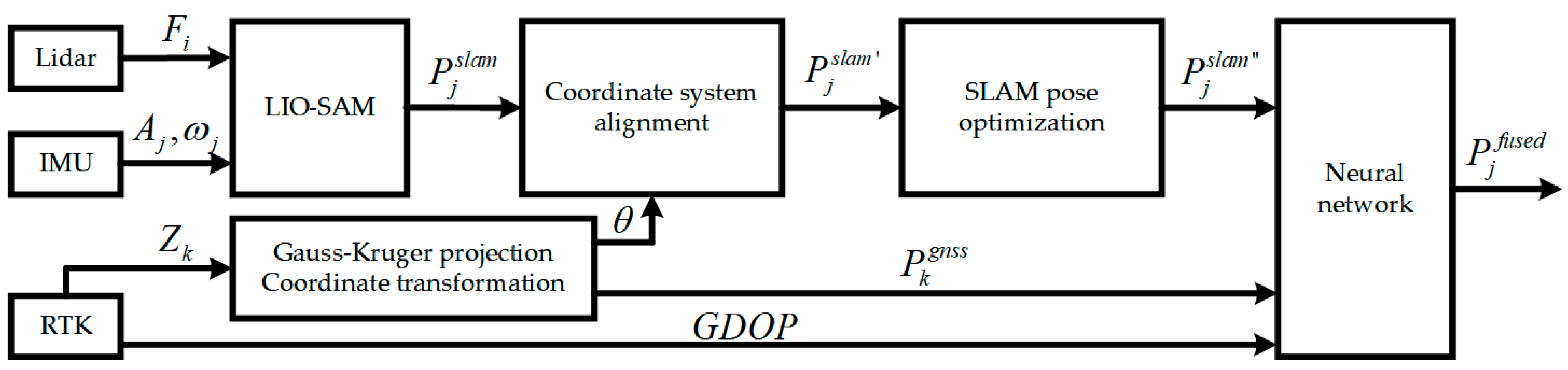
2.1. Algorithm Framework

The SLAM/GNSS fusion localization algorithm proposed in this study achieves continuous and precise positioning for robots in weak or GNSS-denied environments by integrating LIO-SAM (tightly-coupled lidar inertial odometry via smoothing and mapping) [29] and dual-antenna RTK-measured positioning and orientation data. This study adopts a loosely coupled approach where the SLAM and GNSS subsystems operate independently. A neural network-based dynamic weight adjustment fusion localization algorithm was designed to perform data integration. The overall framework is illustrated in Figure 1, with the corresponding nomenclature provided in

Table 1. Nomenclature corresponding to Figure 1.

Symbol	Meaning
$F_i$	The point cloud data from LiDAR
$A_j$	The acceleration from IMU
${\omega }_j$	The angular velocity from IMU
$Z_k$	The positioning orientation data from the dual antennas
$\theta$	The initial RTK heading angle
$P_k^{\mathrm{gnss}}$	The observed pose in the GNSS coordinate system
$P_j^{slam}$	The observed pose in the SLAM coordinate system
$P_j^{slam\prime }$	The SLAM pose after preprocessing of coordinate system alignment
$P_j^{slam\prime \prime }$	The optimized SLAM pose
$P_j^{fused}$	The fused pose
i, j, k	The time-series markers of the LiDAR, IMU, and RTK

. First, the point cloud data from LiDAR and the acceleration and angular velocity from the IMU (Inertial Measurement Unit) are coupled into LIO-SAM to obtain the observed pose of the center point of the drive wheel axis in the SLAM coordinate system. Subsequently, the real-time dynamically measured positioning orientation data from the dual antennas are subjected to Gauss–Kruger projection and coordinate transformation to obtain the observed pose of the center point of the drive wheel axis in the GNSS coordinate system. Then, coordinate system alignment preprocessing is implemented to unify the coordinate system of multi-sensor observed poses, followed by outlier filtering and drift correction to optimize the SLAM poses. Finally, the observed poses from two distinct coordinate systems and the GDOP are fed into the neural network model to dynamically adjust the optimization weights of each observed pose, thereby outputting the fused pose.

2.2. SLAM/GNSS Fusion Localization Algorithm

2.2.1. LiDAR-Inertial Odometry

This research employs the LIO-SAM algorithm for state estimation. This algorithm constructs a factor graph optimization framework, as shown in Figure 2, incorporating four key factors: the IMU pre-integration factor, LiDAR odometry factor, GPS factor, and loop closure factor. By applying nonlinear optimization methods to optimize the factor graph, the system achieves globally consistent robot poses, enabling high-precision state estimation and map construction.

The IMU pre-integration factor efficiently computes the relative motion increments between consecutive LiDAR keyframes i and i + 1 by pre-integrating IMU data. These increments include positional increment $\mathsf{\Delta }{P}_{i,i+1}$, velocity increment $\mathsf{\Delta }{V}_{i,i+1}$, and rotational increment $\mathsf{\Delta }{R}_{i,i+1}$, which are incorporated as constraints into the factor graph for optimization. The IMU pre-integration formulation is expressed as follows:

$$\left\{\begin{array}{l}\mathsf{\Delta }{V}_{i,i+1}=R_i^T\left(V_{i+1}-V_i-g\mathsf{\Delta }{t}_{i,i+1}\right)\\ \mathsf{\Delta }{P}_{i,i+1}=R_i^T\left(P_{i+1}-P_i-V_i\mathsf{\Delta }{t}_{i,i+1}-{\displaystyle \frac{1}{2}}g\mathsf{\Delta }{t}_{i,i+1}^2\right)\\ \mathsf{\Delta }{R}_{i,i+1}=R_i^T{R}_{i+1}\end{array}\right.$$

(1)

where g is the acceleration of gravity; $\mathsf{\Delta }{t}_{i,i+1}$ is the time interval between two neighboring keyframes; $V_i$ and $V_{i+1}$ are the velocities at the moments i and i + 1; $P_i$ and $P_{i+1}$ are the positions at the moments i and i + 1; $R_i^T$ is the rotation matrix transpose at the moment i; and $R_{i+1}$ is the rotation matrix at the moment i + 1.

The LiDAR odometry factor first extracts features from preprocessed point cloud data using a curvature-based method, categorizing them into edge features and planar features, while introducing the concept of LiDAR keyframes. A sliding window approach is then employed to construct a point cloud map containing a fixed number of recent LiDAR scans. Finally, the point-to-edge distance $d_{e_k}$ and point-to-plane distance $d_{p_k}$ are utilized to formulate pose estimation equations.

$$\left\{\begin{array}{l}{d}_{e_k}={\displaystyle \frac{\left|\left(p_{i+1,k}^e-p_{i,u}^e\right)\times \left(p_{i+1,k}^e-p_{i,v}^e\right)\right|}{\left|p_{i,u}^e-p_{i,v}^e\right|}}\\ d_{p_k}={\displaystyle \frac{\left|\begin{array}{c}\left(p_{i+1,k}^p-p_{i,u}^p\right)\\ \left(p_{i,u}^p-p_{i,v}^p\right)\times \left(p_{i,u}^p-p_{i,w}^p\right)\end{array}\right|}{\left|\left(p_{i,u}^p-p_{i,v}^p\right)\times \left(p_{i,u}^p-p_{i,w}^p\right)\right|}}\end{array}\right.$$

(2)

where k, u, v, and w are feature indices in the corresponding set; $p_{i+1,k}^e$, $p_{i,u}^e$, and $p_{i,v}^e$ are points on edge features; and $p_{i+1,k}^p$, $p_{i,u}^p$, $p_{i,v}^p$, and $p_{i,w}^p$ are points on planar features.

The Gauss–Newton method is used to solve for the optimal transformation by minimizing:

$$\underset{T_{i+1}}{\min }\left\{{\displaystyle \sum _{p_{i+1,k}^e\in \prime F_{i+1}^e}{d}_{e_k}}+{\displaystyle \sum _{p_{i+1,k}^p\in \prime F_{i+1}^p}{d}_{p_k}}\right\}$$

(3)

where $T_{i+1}$ is the pose at moment i + 1; $\prime F_{i+1}^e$ is the edge feature transformed to the world coordinate system; and $\prime F_{i+1}^p$ is the planar feature transformed to the world coordinate system.

The relative pose transformation between two adjacent keyframes is computed:

$$\mathsf{\Delta }{T}_{i,i+1}=T_i^T{T}_{i+1}$$

(4)

where $T_i$ is the pose at moment i.

The GPS factor provides global positional constraints to the system by integrating GPS measurement data. Upon receiving GPS observations, the data are transformed into a local Cartesian coordinate system. When new nodes are added to the factor graph, the corresponding GPS factor is associated with these nodes to establish spatial constraints.

The loop closure factor employs a simple yet effective Euclidean distance-based detection method. The algorithm first searches historical keyframes to identify candidate loop closure frames that are temporally distant but spatially proximate. Subsequently, scan-to-map optimization is performed to estimate the relative pose transformation between the current keyframe and the candidate frame. This transformation is then incorporated as a loop closure factor into the factor graph for global trajectory optimization.

2.2.2. Coordinate System Alignment

The SLAM coordinate system is defined with its origin at the initial position of the center point of the drive wheel axis. Its positive X-axis aligns with the robot’s forward direction, while the positive Y-axis is oriented towards the robot’s left side, following the right-hand rule. The GNSS coordinate system shares the same origin but adopts an ENU (East-North-Up) frame convention, with the positive X-axis pointing to geodetic east and the positive Y-axis to geodetic north. The arbitrary initial orientation of the robot typically results in a fixed angular deviation θ about the Z-axis between the SLAM and GNSS coordinate systems, as shown in Figure 3. To enable fusion of observed poses from these two distinct coordinate systems, coordinate system alignment is required.

During the system initialization phase, the initial heading angle θ is obtained through dual-antenna RTK measurements. The SLAM coordinate system is then rotated about the Z-axis by −θ to align with the GNSS coordinate system, resulting in an intermediate coordinate system MID that serves as the base coordinate system for SLAM. By establishing the coordinate transformation relationship from the SLAM coordinate system to the MID coordinate system, positional coordinates in the SLAM coordinate system can be transformed into the MID coordinate system, thereby achieving unification of the coordinate system for multi-sensor observed poses. The transformation is formulated as follows:

$$\left[\begin{array}{l}{x}_{mid}\\ y_{mid}\\ z_{mid}\end{array}\right]=R_{SLAM}^{MID}\left[\begin{array}{l}{x}_{slam}\\ y_{slam}\\ z_{slam}\end{array}\right]=\left[\begin{array}{ccc}\cos \left(-\theta \right)& -\sin \left(-\theta \right)& 0\\ \sin \left(-\theta \right)& \cos \left(-\theta \right)& 0\\ 0& 0& 1\end{array}\right]\left[\begin{array}{l}{x}_{slam}\\ y_{slam}\\ z_{slam}\end{array}\right]$$

(5)

where $x_{slam}$, $y_{slam}$, and $z_{slam}$ are the position coordinates under the SLAM coordinate system; $x_{mid}$, $y_{mid}$, and $z_{mid}$ are the position coordinates under the MID coordinate system; and $R_{SLAM}^{MID}$ is the rotation matrix from the SLAM coordinate system to the MID coordinate system.

2.2.3. SLAM Pose Optimization

During the implementation of the LIO-SAM algorithm for simultaneous localization and mapping, sporadic localization outliers may emerge in the LiDAR-inertial odometry. These localization outliers, characterized by abrupt pose jumps at specific timestamps, often result from dynamic object interference, sensor noise, or feature matching errors. These localization outliers must be filtered out to enhance the system’s temporal continuity and operational stability. The pose outlier detection proceeds by first computing the Euclidean displacement between the current and previous poses in the SLAM coordinate frame. If this displacement exceeds a predefined threshold, the current pose is identified as an outlier. The system then substitutes the outlier with a linearly extrapolated pose derived from the previous pose data, as formalized below:

$$\left\{\begin{array}{l}{x}_t=x_{t-1}+k_x^{t-1}\mathsf{\Delta }t\\ y_t=y_{t-1}+k_y^{t-1}\mathsf{\Delta }t\\ {\theta }_t={\theta }_{t-1}+k_{\theta }^{t-1}\mathsf{\Delta }t\end{array}\right.$$

(6)

where $x_t$, $y_t$, and ${\theta }_t$ are the x, y coordinates and heading angle at the current moment; $x_{t-1}$, $y_{t-1}$, and ${\theta }_{t-1}$ are the x, y coordinates and heading angle at the previous moment; $k_x^{t-1}$, $k_y^{t-1}$, and $k_{\theta }^{t-1}$ are the rate of change of x, y coordinates and heading angle at the previous moment; and $\mathsf{\Delta }t$ is the time interval between the current moment and the previous moment.

GNSS data are not entered into the LIO-SAM framework because LIO-SAM does not fully utilize GNSS information [30]. The radar inertial odometers may have accumulated errors due to drift during long time operation of the system. When the quality of the GNSS signal is high, the drift of the radar inertial odometer can be suppressed by using the coordinate data under the GNSS coordinate system as a global position constraint, thus reducing the cumulative error and improving the stability of the system. When RTK has a fixed solution and the GNSS signal quality is high, the difference between the pose in the GNSS coordinate system and the pose in the SLAM coordinate system is calculated. When the difference exceeds the set distance threshold or angle threshold, the position coordinates are corrected in the SLAM coordinate system. Since this is designed for wheeled robots moving on a plane, we only consider distance deviations in the X and Y directions and heading angle deviation. The correction formula is as follows:

$$\left\{\begin{array}{l}{x}_{mix}=x+\mathsf{\Delta }x\\ y_{mix}=y+\mathsf{\Delta }y\\ {\theta }_{mix}=\theta +\mathsf{\Delta }\theta \end{array}\right.$$

(7)

where $x_{mix}$, $y_{mix}$, and ${\theta }_{mix}$ are the x, y coordinates and heading angles after correction; $x$, $y$, and $\theta$ are the x, y coordinates and heading angles before correction; and $\mathsf{\Delta }x$, $\mathsf{\Delta }y$, and $\mathsf{\Delta }\theta$ are the x, y coordinates and heading angle differences.

2.2.4. Neural Network-Based Dynamic Weight Adjustment

LIO-SAM assigns fixed observation weights to both GNSS and LiDAR odometry [30]. However, in practical scenarios, the signal quality of GNSS significantly differs between open and obstructed environments. The fixed-weight strategy fails to adequately account for the environmental sensitivity of GNSS signal quality, resulting in high-quality observations not being fully leveraged. Given the powerful adaptive and nonlinear mapping capabilities of neural networks, this study proposes a neural network model with dynamic weight adjustment. It adaptively adjusts the weights of poses from two distinct coordinate systems based on the magnitude of GDOP through end-to-end training, aiming to achieve the fusion of SLAM and GNSS poses.

The structure of the neural network model is shown in Figure 4. The input layer contains 5-dimensional features: the 2D SLAM position coordinates after preprocessing of coordinate system alignment, 2D GNSS position coordinates, and the GDOP. The first and second hidden layers are fully connected layers with 128 neurons each, using the ReLU (Rectified Linear Unit) as the activation function for feature extraction. The third hidden layer is also a fully connected layer with 64 neurons and ReLU activation, designed to further compress features. The fourth weight generation layer is a fully connected layer with 2 neurons, employing the Softmax function as the activation function to output normalized weights for GNSS and SLAM poses. The fifth fusion layer is a parameter-free mathematical operation layer that performs weighted summation of SLAM and GNSS position coordinates to output the fused position coordinates. The fusion formula is as follows:

$$\left\{\begin{array}{l}{x}_{fused}=w_{gnss}{x}_{gnss}+w_{slam}{x}_{slam}\\ y_{fused}=w_{gnss}{y}_{gnss}+w_{slam}{y}_{slam}\\ w_{gnss}+w_{slam}=1\end{array}\right.$$

(8)

where $w_{gnss}$ is the weight of the GNSS position; $w_{slam}$ is the weight of the SLAM position; $x_{gnss}$ and $y_{gnss}$ are the position coordinates in the GNSS coordinate system; $x_{slam}$ and $y_{slam}$ are the position coordinates in the SLAM coordinate system; and $x_{fused}$ and $y_{fused}$ are the fused position coordinates.

The pseudocode for the neural network-based dynamic weight adjustment algorithm is shown in Algorithm 1. The raw GPS and SLAM coordinates as well as GDOP undergo normalization processing and then pass through three fully-connected layers with ReLU activation for feature extraction. A subsequent weight generation layer generates Softmax-normalized outputs that ensure weights sum to unity. The final fused position combines GPS and SLAM coordinates using these dynamically predicted weights. This architecture dynamically adjusts sensor contributions based on real-time GNSS signal quality while maintaining computational efficiency through compact design choices. The complete system operates within embedded platform constraints for dynamic sensor fusion in agricultural robotics.

Algorithm 1. The pseudocode for the neural network-based dynamic weight adjustment algorithm.

Input: M, $\mu$, $\sigma$, $gp{s}_x$, $gp{s}_y$, $sla{m}_x$, $sla{m}_y$, GDOP Output: $W_{gps}$, $W_{slam}$, $fuse{d}_x$, $fuse{d}_y$   1: function PredictWeights (M, $\mu$, $\sigma$, $gp{s}_x$, $gp{s}_y$, $sla{m}_x$, $sla{m}_y$, GDOP)   2: x $\leftarrow$ [$gp{s}_x$, $gp{s}_y$, $sla{m}_x$, $sla{m}_y$, GDOP]   3: if $\mu \ne \varnothing \wedge \sigma \ne \varnothing$ then   4: x $\leftarrow (x-\mu )\oslash \sigma$   5: end if   6: X $\leftarrow$ tensor(x)   7: ($W_{gps}$, $W_{slam}$) $\leftarrow$ M(X)   8: return $W_{gps}$, $W_{slam}$   9: end function 10: function  FusePosition ($gp{s}_x$, $gp{s}_y$, $sla{m}_x$, $sla{m}_y$, $W_{gps}$, $W_{slam}$) 11: $fuse{d}_x$ $\leftarrow$ $W_{gps}\times gp{s}_x+W_{slam}\times sla{m}_x$ 12: $fuse{d}_y$ $\leftarrow$ $W_{gps}\times gp{s}_y+W_{slam}\times sla{m}_y$ 13: return $fuse{d}_x$, $fuse{d}_y$ 14: end function

This study adopts the MAE (mean absolute error) as the loss function, which computes the mean absolute error $L_{MAE}$ between the fused position coordinates and the ground truth position coordinates. The mathematical formulation is defined as follows:

$$L_{MAE}={\displaystyle \frac{1}{N}}{\displaystyle \sum _{i=1}^N\left|p_{fused}^i-p_{true}^i\right|}$$

(9)

where $p_{fused}^i$ is the fusion position coordinate of the i-th sample; $p_{true}^i$ is the ground truth position coordinate of the i-th sample; and N is the total number of samples.

The training dataset was collected in real-world environments by controlling the robot to maneuver repeatedly between open and obstructed areas. During this process, 5-dimensional input data were continuously recorded, while 2-dimensional ground truth output data were acquired using a total station. After temporal synchronization, the raw data were processed to create a custom dataset, which was then split into 70% for training, 20% for validation, and 10% for testing.

Finally, the fused heading angle is obtained by performing a weighted summation of the SLAM and GNSS heading angles. The fusion formula is defined as follows:

$${\theta }_{fused}=w_{gnss}{\theta }_{gnss}+w_{slam}{\theta }_{slam}$$

(10)

where ${\theta }_{gnss}$ is the heading angle in the GNSS coordinate system; ${\theta }_{slam}$ is the heading angle in the SLAM coordinate system; and ${\theta }_{fused}$ is the fused heading angle.

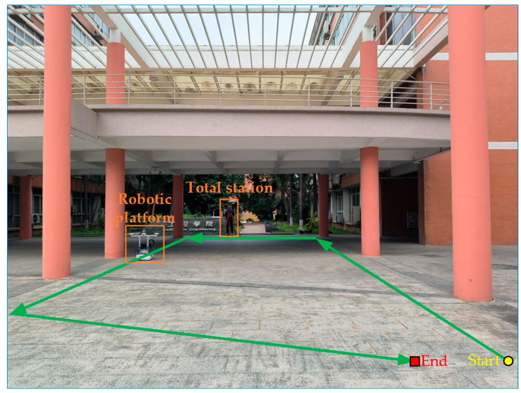
2.3. Robotic Platform Experiments

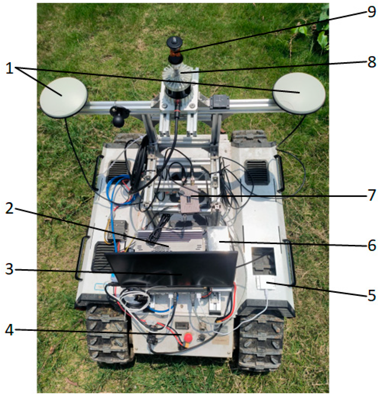
2.3.1. Experimental Platform

To preliminarily validate the performance of the SLAM/GNSS fusion localization algorithm, a robotic platform was developed based on the wheeled differential chassis (AgileX TRACER MINI, Dongguan, China), with its physical prototype shown in Figure 5. The hardware components of the platform include a Yentek G3750F-P4 embedded industrial computer (Intel i9-13900 processor, 32GB RAM, Shenzhen, China); Unicorecomm UM982 satellite receiver (10 Hz output frequency, horizontal positioning accuracy: 0.8 cm + 1 ppm, heading accuracy: 0.1° per 1 m baseline, Yantai, China); WHEELTEC N100 IMU (400 Hz output frequency, accelerometer/gyroscope/magnetometer linearity < 0.1%, Dongguan, China); Ouster OS1 3D LiDAR (10 Hz point cloud output, 128 scan lines, San Francisco, CA, USA); display screen; and 24 V power supply. The software component consists of a localization system based on the SLAM/GNSS fusion localization algorithm. This system is developed within the ROS (Robot Operating System) framework using C++ and deployed on the embedded industrial computer. The satellite receiver’s positioning and heading data, along with the IMU’s inertial attitude data, are input to the localization system via serial port, while the LiDAR’s point cloud data are streamed via ethernet. The localization system employs neural networks to perform multi-sensor data fusion, continuously outputting the robot’s fused pose.

2.3.2. Experimental Protocol

The robotic platform experiments were conducted at the College of Engineering, South China Agricultural University, with the experimental scenario shown in Figure 6. A Leica MS60 total station in automated tracking mode was utilized to record the robot’s ground truth position coordinates in real-time by tracking a prism mounted on the robot. The total station operates at a 10 Hz measurement frequency, achieving a positioning error of 1 mm within a 100 m range. A rectangular path was planned with the starting point set in an area of high GNSS signal quality to facilitate coordinate system alignment during the system initialization phase. The robot was remotely controlled to approximately follow the predefined path, transitioning from GNSS-available zones to GNSS-denied zones, then back to GNSS-available zones. During the robot’s walking process, the position coordinates in the GNSS coordinate system, position coordinates in the SLAM coordinate system, and fused position coordinates output from the localization system were recorded in real-time. Three repeated trials were conducted under identical experimental conditions. Following temporal synchronization and uniform time sampling of the data, the following metrics were calculated: the average position deviation $\overline{d}$ throughout the whole process, the average position deviation ${\overline{d}}_1$ in areas of high GNSS signal quality, the average position deviation ${\overline{d}}_2$ in transitional zones experiencing signal degradation or recovery, the average position deviation ${\overline{d}}_3$ in GNSS-denied environments, and the average velocity $\overline{v}$. These metrics were used to evaluate the localization accuracy and stability of the SLAM/GNSS fusion localization algorithm.

2.4. Orchard Experiments

2.4.1. Experimental Platform

To investigate the operational performance of the SLAM/GNSS fusion localization algorithm in actual orchard terrains and tree-obstructed environments, the aforementioned software and hardware systems were ported to a tracked differential chassis (AgileX BUNKER, Dongguan, China). Its key technical specifications are summarized in

Table 2. Key technical specifications of tracked differential chassis.

Parameters	Value
$\mathrm{Length} \times$$\mathrm{Width} \times$$\mathrm{Height}/(\mathrm{m}\mathrm{m}\times \mathrm{m}\mathrm{m}\times \mathrm{m}\mathrm{m}$)	1023 × 778 × 400
$\mathrm{Total} \mathrm{Mass}/\mathrm{k}\mathrm{g}$	130
$\mathrm{Max} \mathrm{Speed}/(\mathrm{m}\cdot {\mathrm{s}}^{-1}$)	1.5
$\mathrm{Min} \mathrm{Turning} \mathrm{Radius}/\mathrm{m}\mathrm{m}$	0
Max Gradeability/°	30
$\mathrm{Ground} \mathrm{Clearance}/\mathrm{m}\mathrm{m}$	560

, and the physical prototype is shown in Figure 7.

2.4.2. Experimental Protocol

The orchard experiments were conducted at the Horticultural Teaching and Research Base of South China Agricultural University, with the experimental scenario depicted in Figure 8. A rectangular path was planned with the starting point positioned in a GNSS high signal quality area to facilitate coordinate system alignment during initialization. The robot was remotely controlled to approximately follow the predefined path. Throughout the traversal, both the fused position coordinates from the localization system and the ground truth position coordinates from the total station were recorded in real-time. Three repeated trials were conducted under identical experimental conditions. Following temporal synchronization and uniform time sampling of the data, the following metrics were calculated: the average position deviation $\overline{d}$ throughout the whole process, the average position deviation ${\overline{d}}_1$ in areas of high GNSS signal quality, the average position deviation ${\overline{d}}_2$ in transitional zones experiencing signal degradation or recovery, the average position deviation ${\overline{d}}_3$ in GNSS-denied environments, and the average velocity $\overline{v}$. These metrics were utilized to evaluate the localization accuracy and stability of the SLAM/GNSS fusion localization algorithm in actual orchard terrains and tree-obstructed environments.

3. Results and Discussion

3.1. Analysis of Neural Network Model Training Results

The training and validation loss curves of the neural network model are shown in Figure 9. The model was trained using the Adam optimizer with a learning rate of 0.001, with a batch size of 32, and for 300 epochs. The curves demonstrate robust convergence characteristics: both losses decrease rapidly within the first 50 epochs, then plateau along near-parallel trajectories beyond epoch 50, indicating low overfitting risk. This efficient convergence is attributable to the optimized hyperparameter configuration, where the Adam optimizer coupled with ReduceLROnPlateau decay effectively balances convergence speed and stability.

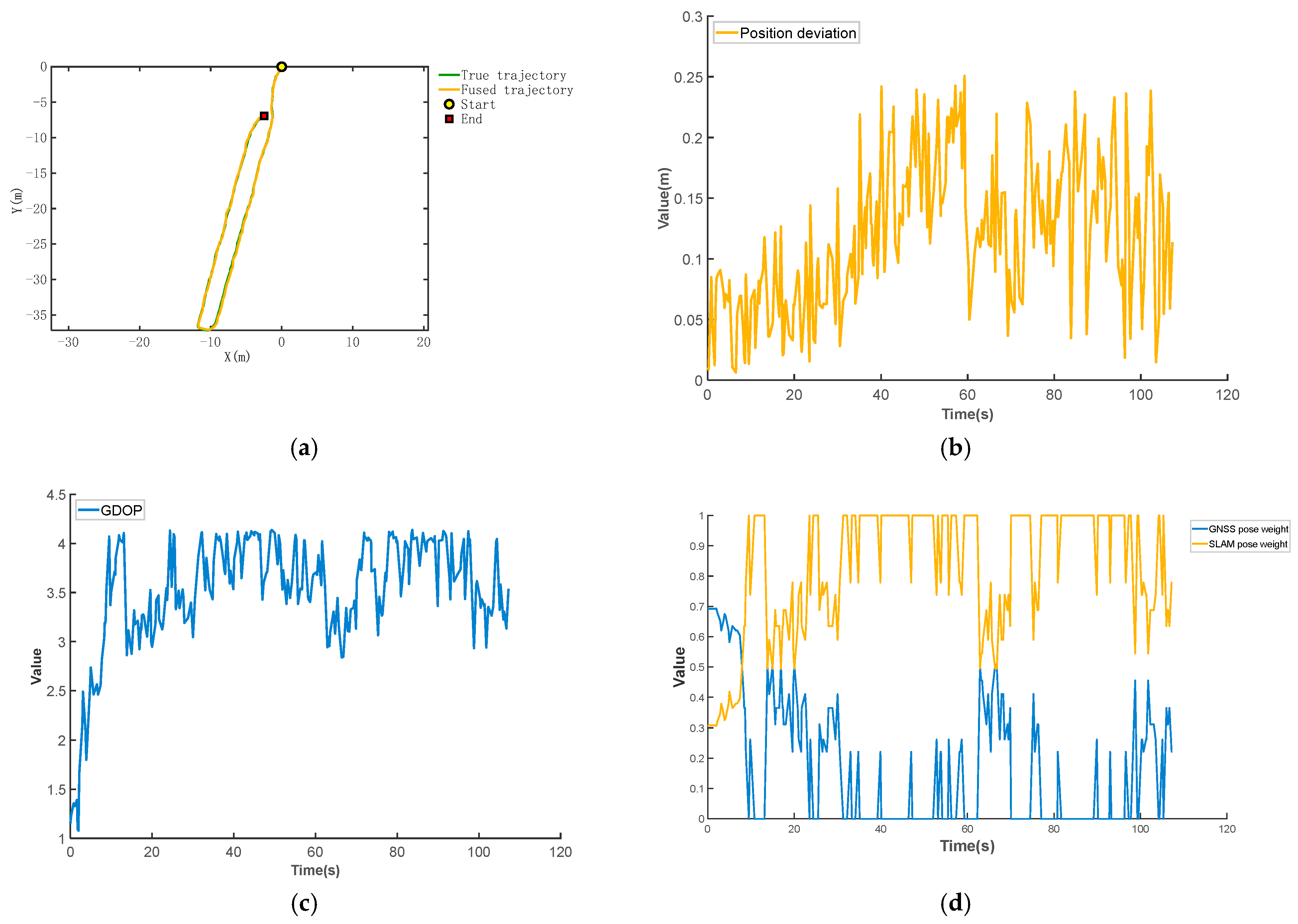
3.2. Analysis of Robotic Platform Experimental Results

The fused trajectory versus the ground truth trajectory from the robotic platform experiment 1 is shown in Figure 10a. The position deviation over time for the localization system employing the SLAM/GNSS fusion localization algorithm is shown in Figure 10b. The position deviation over time for the SLAM localization subsystem without pose optimization is shown in Figure 10c. The position deviation over time for the fixed-weight fusion localization system is shown in Figure 10d. The GDOP over time is shown in Figure 10e, while the time-varying weights assigned to SLAM and GNSS poses are shown in Figure 10f.

During the intervals of 0–19.8 s and 65–80 s, the GDOP remained low, indicating high GNSS signal quality. The SLAM/GNSS fusion localization algorithm optimized the SLAM pose through outlier filtering and drift correction. The weights assigned to GNSS and SLAM poses showed not much difference and remained stable, resulting in an average positional deviation of 0.03 m in these segments. During the 19.9–23.5 s interval, the GDOP gradually increased, indicating a progressive degradation in GNSS signal quality. The SLAM/GNSS fusion localization algorithm dynamically adjusted the weights via the neural network, with the GNSS pose weight continuously decreasing while the SLAM pose weight correspondingly increased. This resulted in an average positional deviation of 0.06 m for this segment. During the 60.7–64.9 s interval, the GDOP gradually decreased, indicating a progressive improvement in GNSS signal quality. The SLAM/GNSS fusion localization algorithm dynamically adjusted the weights via the neural network, with the SLAM pose weight continuously decreasing while the GNSS pose weight correspondingly increased. This resulted in an average positional deviation of 0.08 m for this segment. During the 23.8–60.5 s interval, the GDOP exceeded 4, indicating virtually no GNSS signals. The RTK fixed solution was lost and the GNSS pose weight was set to 0, while the SLAM pose weight was assigned a value of 1. The system thus relied solely on LiDAR odometry for localization. This segment exhibited an average positional deviation of 0.11 m with no significant dispersion in localization error, demonstrating stable performance over extended durations.

The results from three repeated trials are summarized in

Table 3. Experimental results of robotic platform.

Experiment NO.	$\overline{\mathit{d}}/\mathbf{m}$	${\overline{\mathit{d}}}_1/\mathbf{m}$	${\overline{\mathit{d}}}_2/\mathbf{m}$	${\overline{\mathit{d}}}_3/\mathbf{m}$	$\overline{\mathit{v}}/(\mathbf{m}·{\mathbf{s}}^{-1})$
1	0.07	0.03	0.07	0.11	0.60
2	0.07	0.04	0.07	0.10	0.54
3	0.06	0.04	0.05	0.08	0.58
Average	0.07	0.04	0.06	0.10	0.57

. The SLAM/GNSS fusion localization algorithm achieved the following metrics: $\overline{d}$ = 0.07 m, ${\overline{d}}_1$ = 0.04 m, ${\overline{d}}_2$ = 0.06 m, ${\overline{d}}_3$ = 0.10 m, and $\overline{v}$ = 0.57 m/s. Compared to the SLAM algorithm without pose optimization, the proposed SLAM/GNSS fusion localization algorithm reduced the whole process’s average position deviation by 37%. Compared to the fixed-weight fusion localization algorithm, the proposed SLAM/GNSS fusion localization algorithm achieved a 74% reduction in average position deviation during transitional segments with GNSS signal degradation or recovery. Experimental results on the robotic platform demonstrate the superior positioning accuracy and stability of the proposed SLAM/GNSS fusion localization algorithm in weak or GNSS-denied environments.

3.3. Analysis of Orchard Experimental Results

The fused trajectory versus the ground truth trajectory from the orchard experiments 1 is shown in Figure 11a. The deviation d between the fused positions and ground truth positions over time is shown in Figure 11b. The GDOP over time is shown in Figure 11c, while the time-varying weights assigned to SLAM and GNSS poses are shown in Figure 11d.

During the 0–9.5 s interval, the robot transitioned from an open area to a tree-obstructed zone. The GDOP gradually increased, indicating a progressive degradation in GNSS signal quality. The SLAM/GNSS fusion localization algorithm dynamically adjusted the weights via the neural network, resulting in a continuous decrease in the GNSS pose weight and a corresponding increase in the SLAM pose weight. During the 9.8–107.3 s interval, the robot operated entirely within a tree-obstructed environment. The GDOP fluctuated between 2.8552 and 4.1664, indicating low and highly fluctuating GNSS signal quality. The SLAM/GNSS fusion localization algorithm dynamically adjusted the pose weights via the neural network, with both GNSS and SLAM weights continuously adapting to real-time GNSS signal quality variations.

The results from three repeated trials are summarized in

Table 4. Orchard experimental results.

Experiment NO.	$\overline{\mathit{d}}/\mathbf{m}$	${\overline{\mathit{d}}}_1/\mathbf{m}$	${\overline{\mathit{d}}}_2/\mathbf{m}$	${\overline{\mathit{d}}}_3/\mathbf{m}$	$\overline{\mathit{v}}/(\mathbf{m}·{\mathbf{s}}^{-1})$
1	0.12	0.06	0.12	0.13	0.67
2	0.11	0.05	0.10	0.15	0.53
3	0.12	0.07	0.11	0.14	0.46
Average	0.12	0.06	0.11	0.14	0.55

. The SLAM/GNSS fusion localization algorithm achieved the following metrics: $\overline{d}$ = 0.12 m, ${\overline{d}}_1$ = 0.06 m, ${\overline{d}}_2$ = 0.11 m, ${\overline{d}}_3$ = 0.14 m, and $\overline{v}$ = 0.55 m/s. Experimental results in the orchard demonstrate that the proposed SLAM/GNSS fusion localization algorithm maintains high localization accuracy and stability even under conditions of low and highly fluctuating GNSS signal quality, meeting the operational requirements of most agricultural robots.

3.4. Discussion

The requirement to position the robot’s starting point in high GNSS signal quality areas for coordinate system alignment during initialization imposes limitations on the applicability of the proposed SLAM/GNSS fusion localization algorithm across diverse operational scenarios.

While this study achieved robust localization in GNSS-degraded or denied environments, atmospheric effects (particularly ionospheric delays) were not addressed. Future work will characterize these impacts using the receiver’s raw multi-frequency signals for real-time atmospheric error correction.

Since the total station cannot directly provide ground truth heading angles for tracked mobile devices, this study omitted heading angle deviation as an experimental metric. Future research could focus on acquiring accurate ground truth heading angles for robots in GNSS-denied environments to further analyze the heading angle accuracy of the proposed SLAM/GNSS fusion localization algorithm.

Typical agricultural machines operate at a speed of 1 to 1.5 m/s, but the experimental average speed described above was only about 0.5 m/s. At velocities exceeding 1 m/s, the algorithm may sacrifice positional precision to maintain real-time performance. Subsequent studies can add high-speed testing scenarios to verify the accuracy and stability of the algorithm at typical farm machine operating speeds.

In real agricultural scenarios, the dust generated during robotic operations and frequent precipitation during the rainy season can have an impact on the point cloud quality of the LiDAR. Suspended particulate matter in the dust scatters the laser light, resulting in noticeable noise. Raindrops reflect and absorb the laser light, resulting in anomalous increases or disappearances in the point cloud. The distortion of LiDAR point cloud data will affect the effectiveness of the algorithm to a certain extent, so in subsequent research we need to consider how to eliminate these effects as much as possible to improve the stability of the algorithm in harsh environments. For example, a waveform recognition algorithm could be used to analyze the reflectivity size and orientation of the noise and set an appropriate threshold to filter the noise, or a deep learning-based denoising method could be used to develop a noise filtering network based on semantic information.

Looking forward, the XAI-based SLAM and deep learning-based localization approaches will drive the development of next-generation agricultural positioning technologies [31]. For example, Tateno et al. [32] propose a method in which CNN-predicted dense depth maps are fused with depth measurements from direct monocular SLAM, resulting in semantically coherent scene reconstruction from a single view. Feng et al. [33] propose the 2D3D-MatchNet, an end-to-end deep network architecture that jointly learns descriptors for 2D and 3D keypoints from images and point clouds for visual pose estimation. While current computational constraints limit their real-time deployment on embedded platforms, emerging edge-compatible architectures and lightweight explainable AI models are rapidly closing this gap. Artificial intelligence-driven multi-modal perception will advance environmental adaptability, promising to further enhance the positioning accuracy and stability of agricultural robots in weak or GNSS-denied environments.

4. Conclusions

To address the issue of agricultural robot loss of control caused by GNSS signal degradation or loss in complex agricultural environments such as farmland and orchards, this study proposes a neural network-based SLAM/GNSS fusion localization algorithm. It achieves multi-sensor observed pose coordinate system unification through coordinate system alignment preprocessing, optimizes SLAM poses via outlier filtering and drift correction, and dynamically adjusts the weights of poses from distinct coordinate systems via a neural network according to the GDOP. These mechanisms collectively enhance the robot’s localization accuracy and stability in weak or GNSS-denied environments.

To preliminarily validate the performance of the SLAM/GNSS fusion localization algorithm, robotic platform experiments were conducted. The experimental results demonstrate that, at an average speed of 0.57 m/s, the proposed SLAM/GNSS fusion localization algorithm achieves an overall average position deviation of 0.07 m, with average position deviation of 0.04 m in areas of high GNSS signal quality, 0.06 m in transitional zones experiencing signal degradation or recovery, and 0.10 m in fully GNSS-denied environments. Compared to the SLAM algorithm without pose optimization, the proposed SLAM/GNSS fusion localization algorithm reduced the whole process average position deviation by 37%. Compared to the fixed-weight fusion localization algorithm, the proposed SLAM/GNSS fusion localization algorithm achieved a 74% reduction in average position deviation during transitional segments with GNSS signal degradation or recovery. These results validate the superior positioning accuracy and stability of the proposed SLAM/GNSS fusion localization algorithm in weak or GNSS-denied environments.

To investigate the operational performance of the SLAM/GNSS fusion localization algorithm in actual orchard terrains and tree-obstructed environments, orchard field experiments were conducted. The experimental results demonstrate that, at an average speed of 0.55 m/s, the proposed SLAM/GNSS fusion localization algorithm achieves an overall average position deviation of 0.12 m, with average position deviation of 0.06 m in high GNSS signal quality zones, 0.11 m in transitional sections under signal degradation or recovery, and 0.14 m in fully GNSS-denied environments. These results validate that the proposed SLAM/GNSS fusion localization algorithm maintains high localization accuracy and stability, even under conditions of low and highly fluctuating GNSS signal quality, meeting the operational requirements of most agricultural robots.

References

1. Luo, X.W.; Hu, L.; He, J.; Zhang, Z.G.; Zhou, Z.Y.; Zhang, W.Y.; Liao, J.; Huang, P.K. Key Technologies and Practice of Unmanned Farm in China. Trans. Chin. Soc. Agric. Eng. 2024, 40, 1–16. [Google Scholar] [CrossRef]
2. Liu, J.Z.; Jiang, Y.X. Industrialization Trends and Multi-arm Technology Direction of Harvesting Robots. Trans. Chin. Soc. Agric. Mach. 2024, 55, 1–17. [Google Scholar] [CrossRef]
3. Sun, Z.Q.; Tang, S.Y.; Luo, X.F.; Dong, J.W.; Xu, N. Research and Application Status of Path Planning for Agricultural Inspection Robots. Agric. Equip. Veh. Eng. 2025, 63, 18–24. [Google Scholar] [CrossRef]
4. Wang, N.; Han, Y.X.; Wang, Y.X.; Wang, T.H.; Zhang, M.; Li, H. Research Progress of Agricultural Robot Full Coverage Operation Planning. Trans. Chin. Soc. Agric. Mach. 2022, 53, 1–19. [Google Scholar] [CrossRef]
5. Zhang, M.; Ji, Y.H.; Li, S.C.; Cao, R.Y.; Xu, H.Z.; Zhang, Z.Q. Research Progress of Agricultural Machinery Navigation Technology. Trans. Chin. Soc. Agric. Mach. 2020, 51, 1–18. [Google Scholar] [CrossRef]
6. Xu, T.; Zhou, Z.Q. Current Status and Trends of Agricultural Robotics Development. Agric. Equip. Technol. 2024, 2025, 51. [Google Scholar]
7. Chen, Y.; Zhang, T.M.; Sun, D.Z.; Peng, X.D.; Liao, Y.Y. Design and experiment of locating system for facilities agricultural vehicle based on wireless sensor network. Trans. Chin. Soc. Agric. Eng. 2015, 31, 190–197. [Google Scholar] [CrossRef]
8. Ma, Q.; Tang, G.Y.; Fu, Z.Y.; Deng, H.G.; Fan, J.N.; Wu, C.C. Research progress on autonomous agricultural machinery technology and automatic parking methods in China. Trans. Chin. Soc. Agric. Eng. 2025, 41, 15–27. [Google Scholar] [CrossRef]
9. Liu, C.L.; Gong, L.; Yuan, J.; Li, Y.M. Development Trends of Agricultural Robots. Trans. Chin. Soc. Agric. Mach. 2022, 53, 1–22, 55. [Google Scholar] [CrossRef]
10. Liu, Z.P.; Zhang, Z.G.; Luo, X.W.; Wang, H.; Huang, P.K.; Zhang, J. Design of automatic navigation operation system for Lovol ZP9500 high clearance boom sprayer based on GNSS. Trans. Chin. Soc. Agric. Eng. 2018, 34, 15–21. [Google Scholar] [CrossRef]
11. Zhang, Z.G.; Luo, X.W.; Zhao, Z.X.; Huang, P.S. Trajectory Tracking Control Method Based on Kalman Filter and Pure Pursuit Model for Agricultural Vehicle. Trans. Chin. Soc. Agric. Mach. 2009, 40, 6–12. [Google Scholar]
12. Ding, Y.C.; He, Z.B.; Xia, Z.Z.; Peng, J.Y.; Wu, T.H. Design of navigation immune controller of small crawler-type rape seeder. Trans. Chin. Soc. Agric. Eng. 2019, 35, 12–20. [Google Scholar] [CrossRef]
13. Li, Q.T.; Liu, B. Design and Path Planning of Agricultural Machinery Automatic Navigation System Based on GNSS. Test. Meas. Technol. 2024, 38, 256–263. [Google Scholar] [CrossRef]
14. Hu, J.T.; Gao, L.; Bai, X.P.; Li, T.C.; Liu, X.G. Review of research on automatic guidance of agricultural vehicles. Trans. Chin. Soc. Agric. Eng. 2015, 31, 1–10. [Google Scholar] [CrossRef]
15. Ji, C.Y.; Zhou, J. Current Situation of Navigation Technologies for Agricultural Machinery. Trans. Chin. Soc. Agric. Mach. 2014, 45, 44–54. [Google Scholar] [CrossRef]
16. Luo, X.W.; Liao, J.; Hu, L.; Zhou, Z.Y.; Zhang, Z.G.; Zang, Y.; Wang, P.; He, J. Research progress of intelligent agricultural machinery and practice of unmanned farm in China. J. South China Agric. Univ. 2021, 42, 8–17. [Google Scholar] [CrossRef]
17. Wang, J.; Chen, Z.W.; Xu, Z.S.; Huang, Z.D.; Jing, J.S.; Niu, R.X. Inter-rows Navigation Method of Greenhouse Robot Based on Fusion of Camera and LiDAR. Trans. Chin. Soc. Agric. Mach. 2023, 54, 32–40. [Google Scholar] [CrossRef]
18. Yousuf, S.; Kadri, M.B. Information Fusion of GPS, INS and Odometer Sensors for Improving Localization Accuracy of Mobile Robots in Indoor and Outdoor Applications. Robotica 2021, 39, 250–276. [Google Scholar] [CrossRef]
19. Yin, X.; Wang, Y.X.; Chen, Y.L.; Jin, C.Q.; Du, J. Development of autonomous navigation controller for agricultural vehicles. Int. J. Agric. Biol. Eng. 2020, 13, 70–76. [Google Scholar] [CrossRef]
20. He, Y.; Huang, Z.Y.; Yang, N.Y.; Li, X.Y.; Wang, Y.W.; Feng, X.P. Research Progress and Prospects of Key Navigation Technologies for Facility Agricultural Robots. Smart Agric. 2024, 6, 1–19. [Google Scholar] [CrossRef]
21. Liu, Y.; Ji, J.; Pan, D.; Zhao, L.J.; Li, M.S. Localization Method for Agricultural Robots Based on Fusion of LiDAR and IMU. Smart Agric. 2024, 6, 94–106. [Google Scholar] [CrossRef]
22. Jin, B.; Li, J.X.; Zhu, D.K.; Guo, J.; Su, B.F. GPS/INS navigation based on adaptive finite impulse response-Kalman filter algorithm. Trans. Chin. Soc. Agric. Eng. 2019, 35, 75–81. [Google Scholar] [CrossRef]
23. Cao, J.J.; Fang, J.C.; Sheng, W.; Bai, H.X. Adaptive neural network prediction feedback for MEMS-SINS during GPS outage. J. Astronaut. 2009, 30, 2231–2236, 2264. [Google Scholar] [CrossRef]
24. Shen, C.; Zhang, Y.; Tang, J.; Cao, H.; Liu, J. Dual-optimization for a MEMS-INS/GPS system during GPS outages based on the cubature Kalman filter and neural networks. Mech. Syst. Signal Process. 2019, 133, 106222. [Google Scholar] [CrossRef]
25. Liu, Q.Y.; Hao, L.L.; Huang, S.J.; Zhu, S.Y. A New Study of Neural Network Aided GPS/MEMS-INS Integrated Navigation. J. Geomat. Sci. Technol. 2014, 31, 336–341. [Google Scholar] [CrossRef]
26. Zhang, W.Y.; Wang, J.; Zhang, Z.G.; He, J.; Hu, L.; Luo, X.W. Self-calibrating Variable Structure Kalman Filter for Tractor Navigation during BDS Outages. Trans. Chin. Soc. Agric. Mach. 2020, 51, 18–27. [Google Scholar] [CrossRef]
27. Wei, Y.F.; Li, Q.L.; Sun, Y.T.; Sun, Y.J.; Hou, J.L. Research on Orchard Robot Navigation System Based on GNSS and Lidar. J. Agric. Mech. Res. 2023, 45, 55–61+69. [Google Scholar] [CrossRef]
28. Hu, L.; Wang, Z.M.; Wang, P.; HE, J.; Jiao, J.K.; Wang, C.Y.; Li, M.J. Agricultural robot positioning system based on laser sensing. Trans. Chin. Soc. Agric. Eng. 2023, 39, 1–7. [Google Scholar] [CrossRef]
29. Shan, T.; Englot, B.; Meyers, D.; Wang, W.; Ratti, C.; Rus, D. LIO-SAM: Tightly-coupled Lidar Inertial Odometry via Smoothing and Mapping. In Proceedings of the 2020 IEEE/RSJ International Conference on Intelligent Robots and Systems, Las Vegas, NV, USA, 25–29 October 2020. [Google Scholar] [CrossRef]
30. Liu, H.; Pan, G.S.; Huang, F.X.; Wang, X.; Gao, W. LiDAR-IMU-RTK fusion SLAM method for large-scale environment. J. Chin. Inert. Technol. 2024, 32, 866–873. [Google Scholar] [CrossRef]
31. Jiang, L.; Xu, B.; Husnain, N.; Wang, Q. Overview of Agricultural Machinery Automation Technology for Sustainable Agriculture. Agronomy 2025, 15, 1471. [Google Scholar] [CrossRef]
32. Tateno, K.; Tombari, F.; Laina, I.; Navab, N. CNN-SLAM: Real-Time Dense Monocular SLAM with Learned Depth Prediction. In Proceedings of the 2017 IEEE Conference on Computer Vision and Pattern Recognition, Honolulu, HI, USA, 21–26 July 2017. [Google Scholar] [CrossRef]
33. Feng, M.; Hu, S.; Ang, M.; Lee, G.H. 2D3D-MatchNet: Learning to Match Keypoints Across 2D Image and 3D Point Cloud. arXiv 2019, arXiv:1904.09742. [Google Scholar] [CrossRef]
Figure 1. Framework of the SLAM/GNSS fusion localization algorithm.
Agriculture 15 01612 g001
Figure 2. Factor graph optimization framework of LIO-SAM.
Agriculture 15 01612 g002
Figure 3. Coordinate system framework.
Agriculture 15 01612 g003
Figure 4. Architecture diagram of the neural network-based model.
Agriculture 15 01612 g004
Figure 5. Physical prototype of robotic platform. 1. RTK dual antenna; 2. display screen; 3. embedded industrial computer; 4. IMU 5. wheeled differential chassis; 6. power supply; 7. satellite receiver; 8. LiDAR; 9. prism.
Agriculture 15 01612 g005
Figure 6. Experimental scenario of robotic platform.
Agriculture 15 01612 g006
Figure 7. Physical prototype of orchard platform. 1. RTK dual antenna; 2. embedded industrial computer; 3. display screen; 4. tracked differential chassis; 5. IMU; 6. power supply; 7. satellite receiver; 8. LiDAR; 9. prism.
Agriculture 15 01612 g007
Figure 8. Orchard experimental scenario.
Agriculture 15 01612 g008
Figure 9. Training and validation loss curves of the neural network model.
Agriculture 15 01612 g009
Figure 10. (a) Trajectory comparison from robotic platform experiment 1. (b) Position deviation variation curves of the positioning system using the SLAM/GNSS fusion localization algorithm from robotic platform experiment 1. (c) Position deviation variation curves of the SLAM localization subsystem without pose optimization from robotic platform experiment 1. (d) Position deviation variation curves of the fixed-weight fusion localization system from robotic platform experiment 1. (e) GDOP variation curve from robotic platform experiment 1. (f) Weight Variation Curve from robotic platform experiment 1.
Agriculture 15 01612 g010aAgriculture 15 01612 g010b
Figure 11. (a) Trajectory comparison from orchard experiment 1. (b) Position deviation variation curve from orchard experiment 1. (c) GDOP variation curve from orchard experiment 1. (d) Weight Variation Curve from orchard experiment 1.
Agriculture 15 01612 g011