Improving Winter Wheat Yield Estimation Under Saline Stress by Integrating Sentinel-2 and Soil Salt Content Using Random Forest

Abstract

Accurate estimation of winter wheat yield under saline stress is crucial for addressing food security challenges and optimizing agricultural management in regional soils. This study proposed a method integrating Sentinel-2 data and field-measured soil salt content (SC) using a random forest (RF) method to improve yield estimation of winter wheat in Kenli County, a typical saline area in China’s Yellow River Delta. First, feature importance analysis of a temporal vegetation index (VI) and salinity index (SI) across all growth periods were achieved to select main parameters. Second, yield models of winter wheat were developed in VI-, SI-, VI + SI-, and VI + SI + SC-based groups. Furthermore, error assessment and spatial yield mapping were analyzed in detail. The results demonstrated that feature importance varied by growth periods. SI dominated in pre-jointing periods, while VI was better in the post-jointing phase. The VI + SI + SC-based model achieved better accuracy (R² = 0.78, RMSE = 720.16 kg/ha) than VI-based (R² = 0.71), SI-based (R² = 0.69), and VI + SI-based (R² = 0.77) models. Error analysis results suggested that the residuals were reduced as the input parameters increased, and the VI + SI + SC-based model showed a good consistency with the field-measured yields. The spatial distribution of winter wheat yield using the VI + SI + SC-based model showed significant differences, and average yields in no, slight, moderate, and severe salinity areas were 7945, 7258, 5217, and 4707 kg/ha, respectively. This study can provide a reference for winter wheat yield estimation and crop production improvement in saline regions.

1. Introduction

Soil salinization has emerged as a global environmental and ecological challenge, particularly prevalent in the arid and semi-arid regions of Northern China. The Yellow River Delta in China represents a prominent case where pedogenic environments and anthropogenic inputs have contributed to extensive soil salinization. Since the 1970s, decreased river discharge combined with seawater intrusion has disrupted the terrestrial water–salt balance, establishing a characteristic coastal salinization zone. This phenomenon has induced soil degradation and constrained crop productivity, posing serious challenges to agricultural sustainability and regional economic development [1]. Recent years have witnessed agricultural transformation in this region driven by labor shortages and policy reforms. Notably, cultivation areas of salt-tolerant crops (e.g., cotton) have markedly decreased, while less salt-tolerant crops, particularly winter wheat, have indicated consistent annual expansion [2]. However, suboptimal resource allocation has resulted in the substantial reduction of winter wheat yields in saline areas. Given the national food security strategies and sustainable saline land utilization policies [3], accurate and timely winter wheat yield estimation has become crucial for informing production management decisions, guiding soil remediation efforts, and optimizing cropping patterns.

Compared with traditional manual crop yield assessment method, remote sensing technology is an efficient approach for improving regional yield estimation due to the significant advantages in non-contact, large-scale monitoring capabilities. Various vegetation indexes (VI), including the Normalized Difference Vegetation Index (NDVI), Enhanced Vegetation Index (EVI), Chlorophyll Reflection Index (CCRI), and Normalized Difference Water Index (NDWI), have been extensively and effectively applied in crop yield estimation in typical saline and other areas. Zhu et al. [4] identified EVI during the booting-filling period as the most effective parameter for winter wheat yield estimation in saline areas. Similarly, Satir et al. [5] achieved reliable wheat yield prediction in Mediterranean saline areas using NDVI, NDWI, and other parameters with stepwise linear regression. Shi et al. [6] employed NDVI for evaluating soil improvement and wheat growth under saline stress. To reflect the cumulative growth process of crops, Chen et al. [7] integrated vegetation indexes from multiple periods to establish a summer maize yield model. Zhao et al. [8] further advanced time-series modeling approaches for maize yield estimation. These methods had demonstrated reasonable estimation accuracy, but they often ignored critical growth-limiting factors. Existing studies have enhanced model generalization by incorporating soil variables. For instance, Farhat et al. [9] improved potato yield estimation accuracy by integrating vegetation indexes with soil conductivity and moisture content. Han et al. [10] achieved an accurate estimation at a county level by combining remote sensing and soil data. Mustafa et al. achieved satisfactory prediction accuracy using vegetation and soil data analysis [11]. Addressing field measurement limitations, Karimli et al. [12] inverted soil parameters (salinity, texture, organic carbon) from remote sensing data and achieved a high accuracy for winter wheat yield estimation by integrating these parameters.

Crop yield estimation using remote sensing methods is characterized by three distinctive features: integration of multiple remote sensing parameters, utilization of multi-source data, and utilization of long-term series analysis. In saline areas, crop productivity is constrained by salt stress, which adversely affects dry matter allocation and harvest index [13] to complicate the relationship between vegetation indexes and yield formation. The spatiotemporal heterogeneity of soil salinity further exacerbates this challenge due to its impact on crops varies substantially across different regions and growth periods [14]. These stress factors often lead to estimation errors when relying solely on single parameters. Field surveys of soil salt data can provide valuable parameters, but they are limited when widely promoted and applied. The soil salinity index (SI) is a quantitative descriptor of surface soil salinity for different areas, e.g., the Yellow River Delta, China [15], Nile Delta, and Egypt [16], and various crop growth periods ranging from bare soil periods [17] to vegetation-covered phases [18]. The integration of vegetation indexes, salinity indexes, and soil salt content parameters offer potential for enhancing information dimensionality and complementary advantages [19]. However, the use of salinity indexes and soil salt content as yield estimation components remains relatively insufficient. In this study, based on the relationships between the multiple parameters (e.g., vegetation indexes, salinity indexes, soil salt content) and wheat yield, we employed a random forest regression method, and integrated Sentinel-2 and soil salt content data to improve winter wheat yield estimation under saline stress in a typical coastal saline agricultural region, namely, Kenli County in the Yellow River Delta, China.

2. Materials and Methods

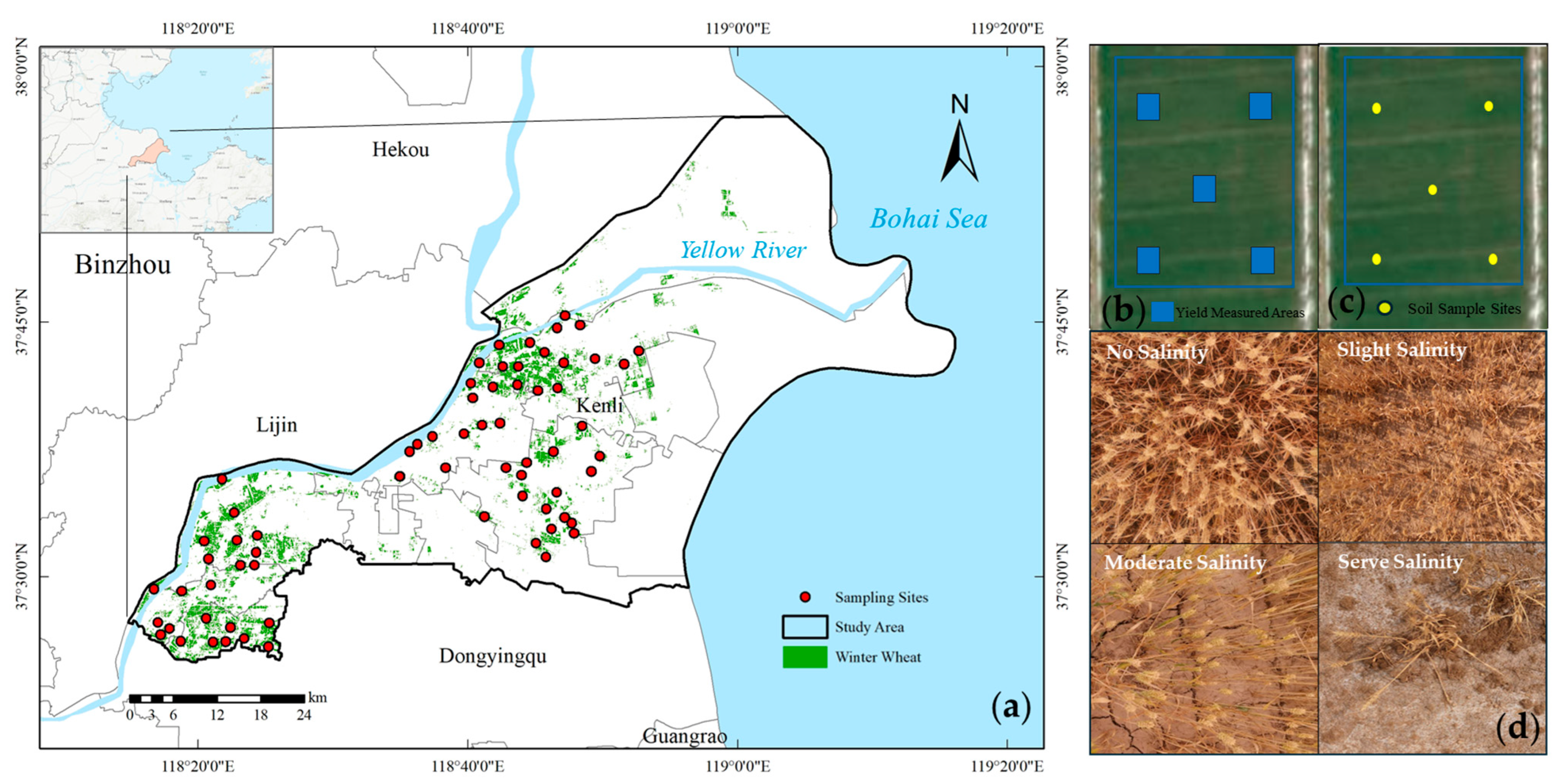
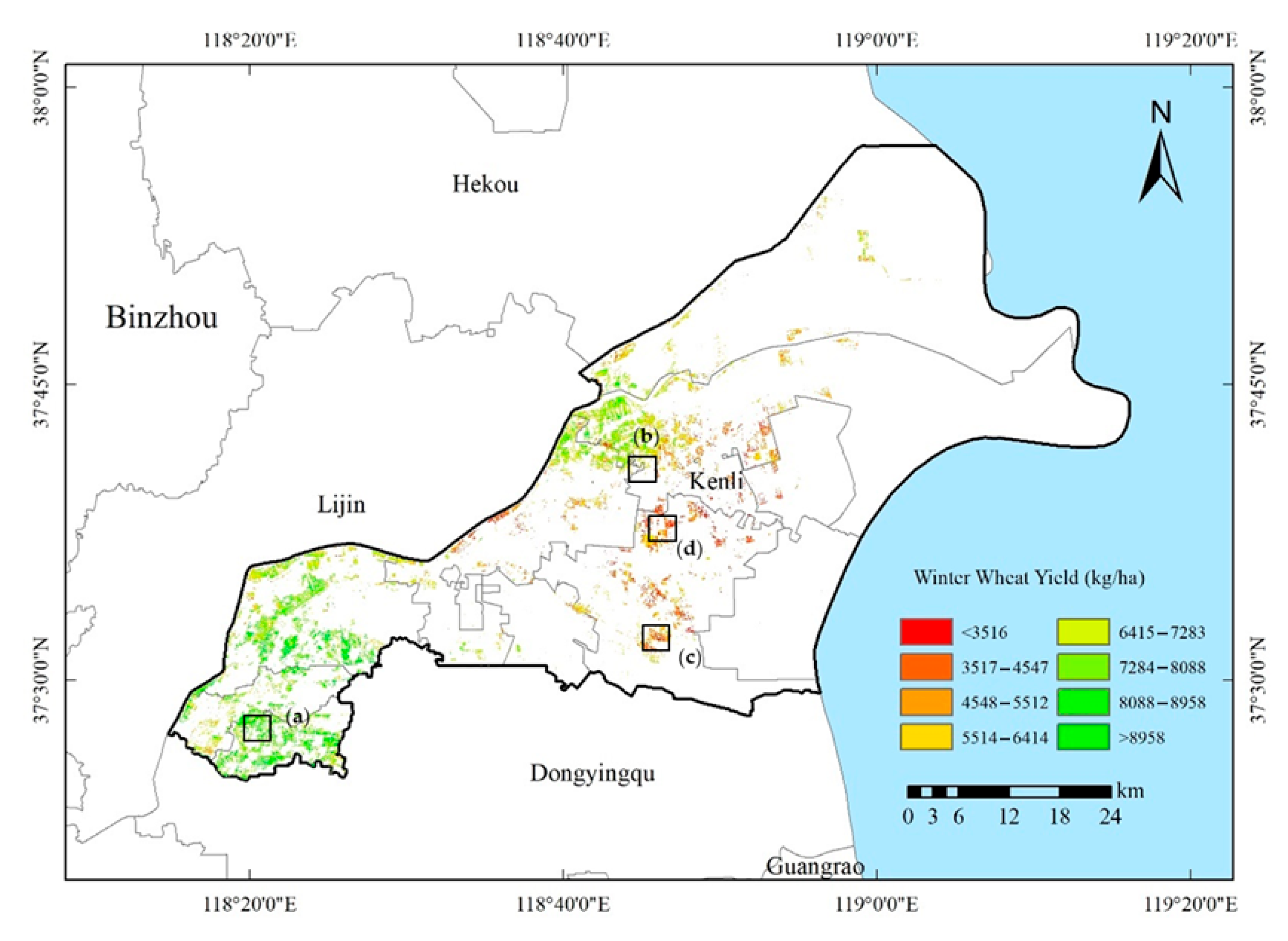
2.1. Study Area

The study area is located in Kenli County, Shandong Province, China, geographically located at 117°90′–119°82′ E and 37°01′–37°99′ N (Figure 1a). The topography is characterized by flat terrain with a gradual southwest-to-northeast slope. This region has a warm temperate semi-humid continental monsoon climate, exhibiting distinct seasonal variations. The area experiences a mean annual temperature of 13.5 °C and receives an average annual precipitation of 555.9 mm. The area has an annual evaporation rate of approximately 1885.0 mm, and the evaporation-to-precipitation ratio reaches about 3.5:1, indicating significant water deficit conditions. This agricultural region primarily cultivates wheat, corn, and cotton. The parent material primarily consists of Yellow River-derived alluvial deposits exhibiting light texture, while surface soils are predominantly classified as sandy loam and light loam. The study area features fluvo-aquic and saline-alkali soils, with chlorides as the dominant salt species. Pronounced spatial heterogeneity has resulted in substantial spatial differences in crop yield distribution. Therefore, we selected this typical county with a distinct environmental gradient for estimating winter wheat yield under saline stress.

2.2. Data Acquisition and Processing

2.2.1. Sampling and Analysis of Winter Wheat and Soil

To ensure an even distribution of samples and meet the request to express spatial variability of soil salinity at county scale, a 10 km² square grid was established to select test plots at the center of each grid cell [20]. For each test plot, winter wheat and soil samples were achieved in June 2024.

Winter wheat yield data were measured in a 10 m × 10 m area to match pixel resolution of remote sensing data, using a five sub-samples quincunx sampling pattern with 1 m² harvest areas per sub-sample (Figure 1b). Winter wheat samples were collected from 68 test plots, and corresponding geographical coordinates were recorded. The harvested winter wheat samples were sun-dried, threshed, and weighed. Then, the yield of per sub-sample was calculated, and the average value was taken as the yield for each sample.

For soil sampling, surface soil samples (0–20 cm depth) were collected at the center location of each sampling grid of winter wheat, as shown in Figure 1c. The collected soil samples were air-dried, passed through a 2 mm sieve, and subsequently prepared as soil-water extracts with a soil-to-water ratio of 5:1. After shaking for 5 min and standing for 8 h, the electrical conductivity (EC) of the soil extracts was measured using a Mettler Toledo FE38 (Mettller Toledo Fe38, Zurich, Swiss) instrument. The measured EC values (mS/cm) were converted to soil salt content (SC, g/kg) according to the conversion formula [21]. Based upon the Chinese soil salinity classification standards [22], the soil salinity levels were categorized as no salinity (<1 g/kg), slight salinity (1–2 g/kg), moderate salinity (2–4 g/kg), and severe salinity (>4 g/kg). The spatial distribution of soil salinity was achieved using an ordinary Kriging interpolation method from the Geostatistical Analyst module in ArcGIS 10.8 (Esri, Redlands, CA, USA) (Figure 2). A Gaussian semivariogram model generated optimal performance (nugget = 0.27727, sill = 0.38282, range = 10.2 km). Model validation using 20% holdout sampling demonstrated satisfactory accuracy (R² = 0.688, RMSE = 0.45 g/kg). While stationarity assumptions may be challenged by the Yellow River Delta’s complex depositional patterns, the sampling design (10 km² grids) captured major salinity gradients. Landscape photos of different salinity levels are shown in Figure 1d and suggested that different salinity levels affected the growth and yield of winter wheat. The sampling sites, soil salt content, and winter wheat yield for each category are indicated in

Table 1. Sample statistic values of different salinity levels.

Salinity Level	Samples	Soil Salt Content (SC) (g/kg)			Winter Wheat Yield (kg/ha)
		Min	Max	Mean	Min	Max	Mean
No	26	0.30	0.99	0.72	6502.23	9904.48	8252.94
Slight	19	1.01	1.98	1.50	4918.38	8641.58	6795.65
Moderate	19	2.01	3.94	2.80	1928.61	8260.78	5368.14
Severe	4	4.38	7.39	5.79	1519.96	3559.61	2660.83

.

2.2.2. Remote Sensing Data

Sentinel-2A/B has a high resolution and revisit period of 5 days. As presented in

Table 2. Spectral bands of the Sentinel-2 sensor.

Bands	Center Wavelength/nm	Resolution/m
Band 1—Coastal aerosol	443	60
Band 2—Blue	490	10
Band 3—Green	560	10
Band 4—Red	665	10
Band 5—Red-edge1	705	20
Band 6—Red-edge2	740	20
Band 7—Red-edge3	783	20
Band 8—NIR	842	10
Band 8A—Narrow NIR	865	20
Band 9—Water Vapor	945	60
Band 10—SWIR Cirrus	1380	60
Band 11—SWIR1	1610	20
Band 12—SWIR2	2190	20

, the primary payload consists of an MSI multispectral imager that covers a spectral range from 440 to 2200 nm and ground resolutions of 10 m (4 bands), 20 m (6 bands), and 60 m (3 bands). Based on the GEE platform (https://earthengine.google.com/ (accessed on 15 November 2024)), 96 images of the 5-day time series of Sentinel-2 from October 2023 to June 2024 were obtained and processed, covering the entire growth cycle of winter wheat. JavaScript programming was employed to calculate Bit10 and Bit11 values in the QA60 cloud information band to obtain the cloud mask and remove cloud interference of remote sensing images.

According to the phenological characteristics of winter wheat in the study area, the growth periods were divided into six periods named P1 to P6 (

Table 3. The number of images used for growth periods of winter wheat.

Growth Periods	Time	Images
P1 (seeding-tiller)	15 October 2023–30 November 2023	25
P2 (dormancy)	9 December 2023–24 February 2024	31
P3 (regreening)	1 March 2024–31 March 2024	15
P4 (jointing)	5 April 2024–20 April 2024	8
P5 (booting-flowering)	26 April 2024–8 May 2024	5
P6 (filling)	12 May 2024–31 May 2024	12

), including seeding-tiller, dormancy, regreening, jointing, booting-flowering, and filling periods. The median synthesis method was used to calculate remote sensing parameters for each growth period.

Vegetation indexes (VIs) can enhance the accuracy of spectral inversion for physiological vegetation and comprehensively reflect information related to crop growth, biomass, and coverage that are associated with crop yield. Six vegetation indexes were calculated from the 13 original bands according to winter wheat characteristics and existing research findings, as depicted in

Table 4. Vegetation indexes and salinity indexes.

Parameters		Formula	References
Vegetation Index (VI)	NDVI	${\displaystyle \frac{(\mathrm{B}8-\mathrm{B}4)}{(\mathrm{B}8 + \mathrm{B}4)}}$	[6]
	EVI	${\displaystyle \frac{2.5 \times (\mathrm{B}8-\mathrm{B}4) }{(\mathrm{B}8+6 \times \mathrm{B}4-7.5 \times \mathrm{B}2+1)}}$	[4]
	CARI	(B5 − B4) − 0.2 × (B5 − B3)	[24]
	CCRI	B8/B5 − 1	[25]
	NDMI	${\displaystyle \frac{(\mathrm{B}8-\mathrm{B}11)}{(\mathrm{B}8+\mathrm{B}11)}}$	[26]
	NDWI	${\displaystyle \frac{(\mathrm{B}3-\mathrm{B}8)}{(\mathrm{B}3+\mathrm{B}8)}}$	[27]
Salinity Index (SI)	SI1	$\sqrt{(\mathrm{B}2 \times \mathrm{B}4)}$	[15]
	SI2	$\sqrt{(\mathrm{B}{3}^2+\mathrm{B}{4}^2)}$	[28]
	SI3	B11/B8	[28]
	SI4	${\displaystyle \frac{(\mathrm{B}4-\mathrm{B}11)}{(\mathrm{B}4+\mathrm{B}11)}}$	[29]
	CRSI	$\sqrt{{\displaystyle \frac{(\mathrm{B}8 \times \mathrm{B}4)-(\mathrm{B}3 \times \mathrm{B}2)}{(\mathrm{B}8 \times \mathrm{B}4)+(\mathrm{B}3 \times \mathrm{B}2)}}}$	[29]

. NDVI and EVI primarily reflected the growth status and nutritional conditions. The chlorophyll absorption reflectance index (CARI) and CCRI were effective in indicating chlorophyll content of crops [23]. The normalized difference moisture index (NDMI) and NDWI performed well in identifying canopy moisture content. The inversion of soil salinity can be indirectly achieved through spectral reflectance. Existing studies have demonstrated that the shortwave infrared and green bands showed high sensitivity to soil salinity, and their combination with the red band could effectively construct a salinity index (SI) that accurately reflect variations of soil salt content. Another SI calculated based on the spectral reflectance of red, blue, and green bands is used to indicate soil salinization in vegetated areas.

2.2.3. Spatial Distribution Data of Winter Wheat

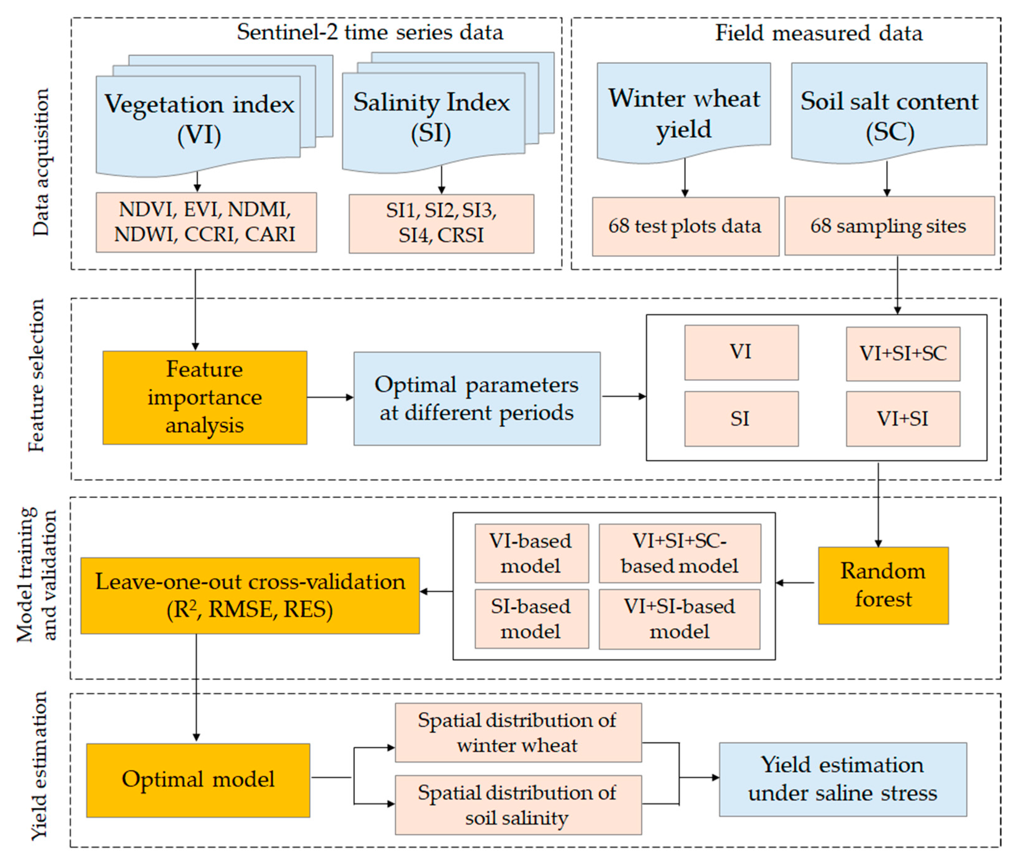
An investigation of land cover distribution in the study area was conducted in April 2024 using a grid-based sampling method. A total of 146 winter wheat samples and 285 non-winter wheat samples were collected, the latter comprising 124 cotton samples, 108 rice samples, and various other land cover types (forest, grassland, and water). All samples were distributed across the main cultivated areas. Based on feature variables (the difference between November NDVI and May NDVI of the following year, NDVI values for May, and the difference between May NDVI and June NDVI), the spatial distribution data of winter wheat in Kenli County in 2024 were produced using a random forest method using data derived from Sentinel-2 temporal variations from Beijing Academy of Agriculture and Forestry Sciences. It can effectively differentiate winter wheat from other vegetation and identify weak information of winter wheat in saline stress areas [30,31]. The confusion matrix is shown in

Table A1. Confusion matrix.

Classes	Winter Wheat	Non-Winter Wheat	Producer Accuracy/%	User Accuracy/%	Overall Accuracy/%	Kappa
Winter wheat	132	18	90.41	88.00	92.45	0.85
Non-winter wheat	14	260	93.53	94.89

. The results suggested that the overall accuracy was 92.45% and the Kappa coefficient was 0.85.

2.3. Method

The flowchart for winter wheat yield estimation in saline stress is illustrated in Figure 3. Using a random forest algorithm, feature importance analysis on vegetation indexes and salinity indexes across various growth periods was performed to select optimal remote sensing parameters. By integrating field-measured soil salt content data, yield estimation models of winter wheat were developed using four variable combinations: VI, SI, VI + SI, and VI + SI + SC. Model accuracy was assessed using the leave-one-out cross validation method, and a comprehensive analysis of estimation residuals was achieved at different salinity levels.

2.3.1. Random Forest

Random forest (RF) is an advanced statistical method based on machine learning, which has exceptional capability in handling high-dimensional datasets and high accuracy of the estimated results [32,33]. Variable importance analysis of random forest provided a robust framework for quantifying the relative contributions of independent parameters [34]. The importance of each parameter on model estimation accuracy was directly quantified using a permutation approach, with lower importance values indicating minor impacts on model performance and higher values reflecting greater influence. While the other three algorithms, namely, XGBoost (eXtreme Gradient Boosting), PLSR (Partial Least Squares Regression), and LSTM (Long Short-Term Memory), offer similar feature analysis, they may suffer from noise sensitivity, inadequate nonlinear modeling, overfitting risks, or computational inefficiencies. RF reduces variance and enhances stability through its Bagging ensemble techniques and random feature selection, demonstrating greater advantages over other methods in small-sample scenarios. In this study, random forest models were employed to select feature parameters and estimate yield of winter wheat.

We established a winter wheat yield estimation model that integrated multiple remote sensing parameters, providing a reliable framework for crop yield estimation. The RF models were implemented using MATLAB software 2016b (MathWorks, Natick, MA, USA). As shown in

Table 5. Random forest parameters by model variant.

Model Variant	Predictors	mtry	ntree	Nodesize
VI-based model	18	6	100	3
SI-based model	13	4	100	3
VI + SI-based model	31	10	100	3
VI + SI + SC-based model	32	10	100	3

, the random forest models for all variants were implemented with consistent hyperparameters: 100 decision trees (ntree), which ensured error stabilization; a minimum leaf size (nodesize) of three to capture detailed patterns while preventing overfitting; and the default mtry value calculated as floor (p/3), where p represents the number of predictors.

2.3.2. Model Validation Method

Given the limited sample size, we employed the leave-one-out cross validation method for model validation. The method offered significant advantages for the limited datasets and maximized data utilization for training to generate robust classifiers [35]. This rigorous approach used a single sample for validation, and the remaining samples were adopted for model training, iterating this process across all samples data. The simulated outputs were subsequently compared with measured values using comprehensive statistical analysis. Model performance was quantitatively assessed using the determination coefficient (R²), root mean square error (RMSE), and residual error (RES), as calculated using the following formulas:

$${\mathrm{R}}^2={\displaystyle \frac{{\sum }_{i=1}^{\mathrm{n}}{\left(\widehat{y_{𝚤}}-\overline{y}\right)}^2}{{\sum }_{i=1}^n{\left(y_i-\overline{y}\right)}^2}}$$

(1)

$$\mathrm{RMSE}=\sqrt{{\displaystyle \frac{1}{n}}{\sum }_{i=1}^{\mathrm{n}}{\left(\widehat{y_{𝚤}}-y_i\right)}^2}$$

(2)

$$\mathrm{RSE}=\widehat{y_{𝚤}}-y_i$$

(3)

where n is the total number of samples, and $y_i$, $\widehat{y_{𝚤}}$, and $\overline{y}$ represent the measured value, estimated value, and the average of the measured values for the samples, respectively.

3. Results

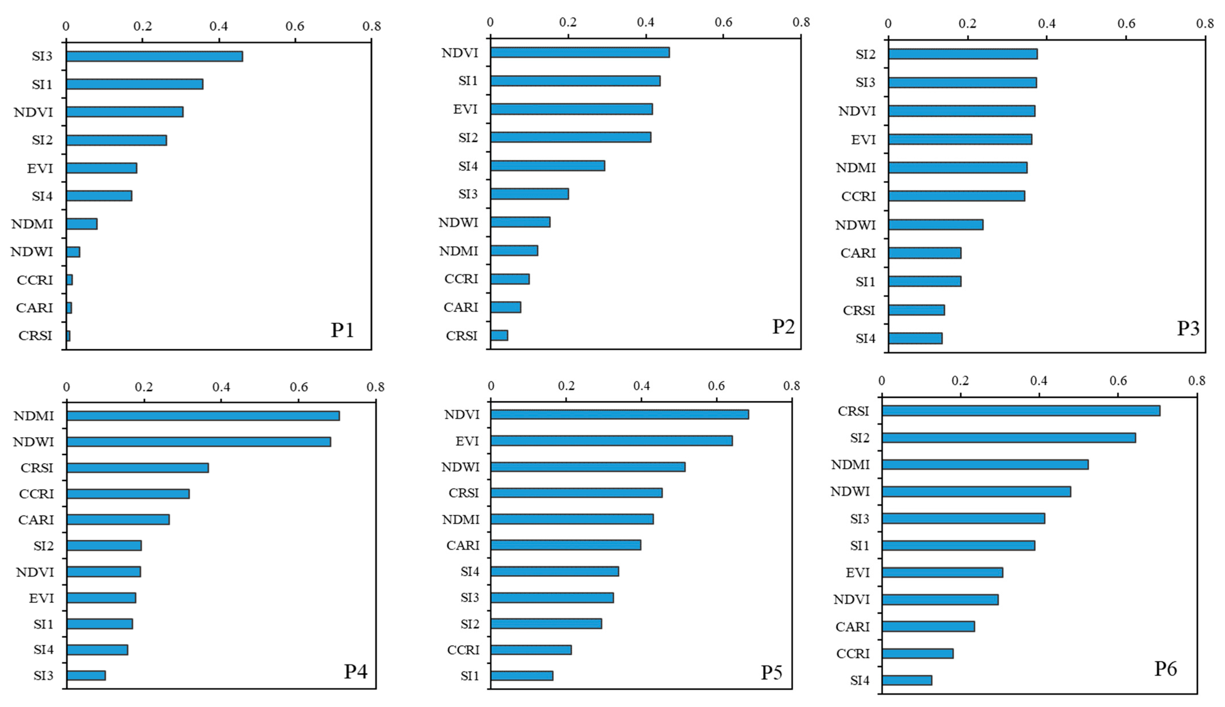
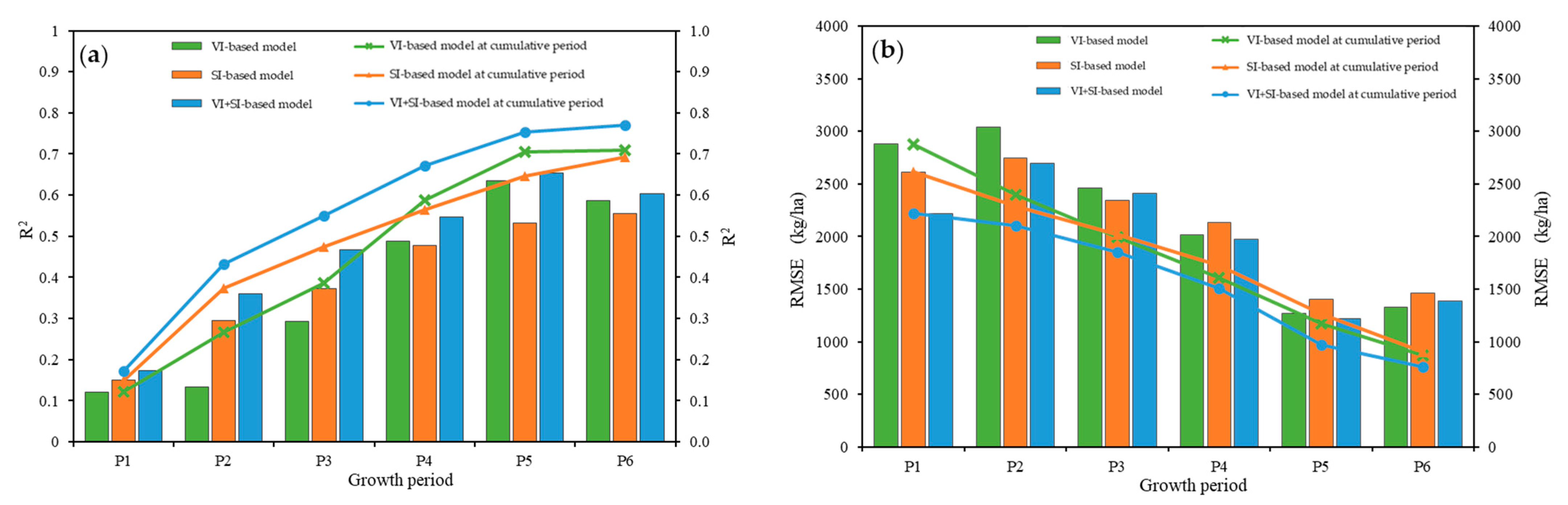
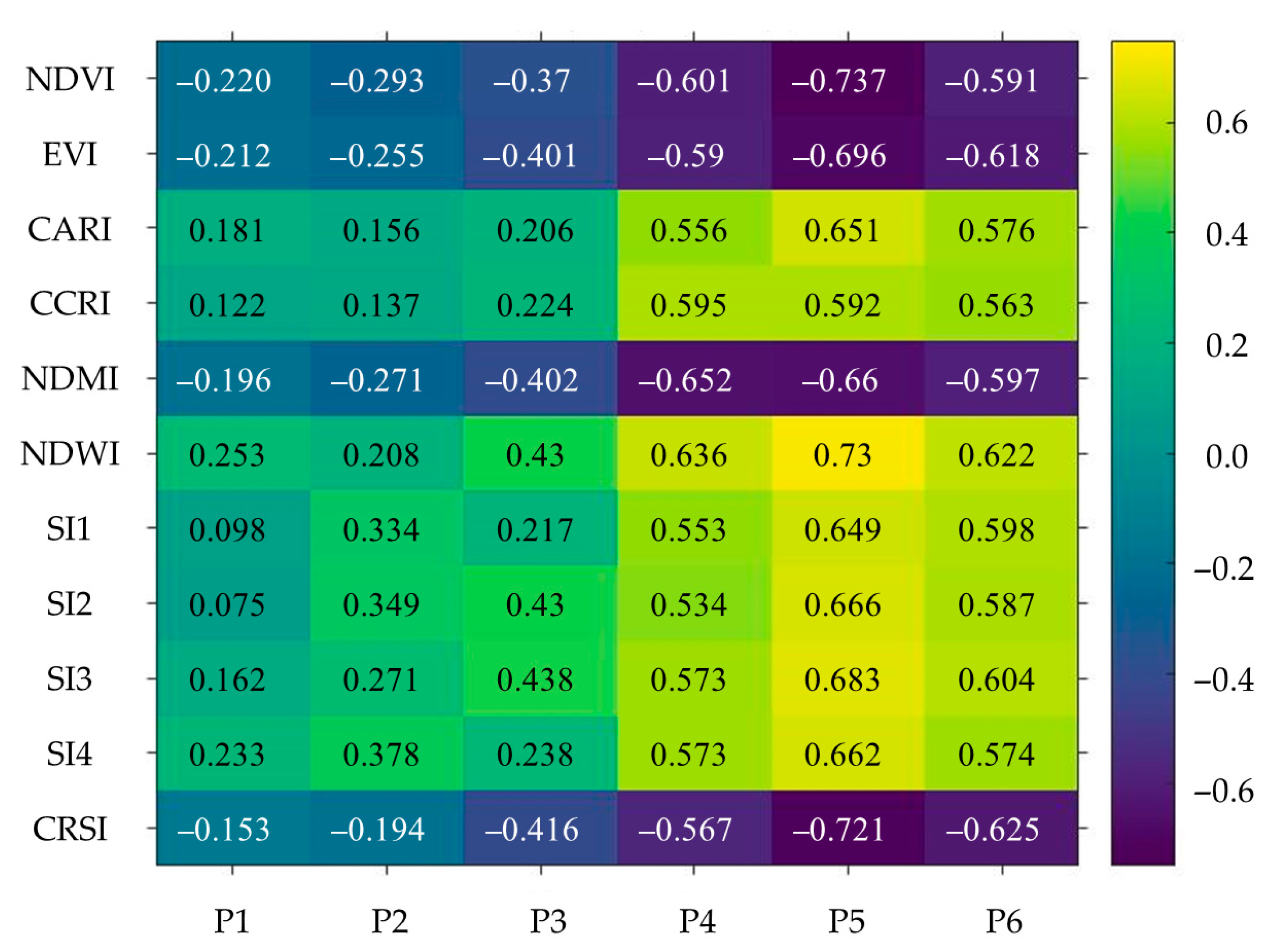
3.1. Feature Parameter Selection in Different Periods

Importance analysis of eleven remote sensing parameters for winter wheat was calculated and sorted in descending order, as shown in Figure 4. The results suggested that the importance of parameters in different growth periods presented distinct patterns. During the seedling-tiller period, SI3 (0.46), SI1 (0.36), NDVI (0.31), and SI2 (0.26) collectively accounted for 73.24% of the total importance. The importance of CCRI, CARI, and CRSI reflected low sensitivity during sparse vegetation periods. For the dormancy period, NDVI (0.46), SI1 (0.44), EVI (0.42), SI2 (0.41), and SI4 (0.29) were key estimative indicators. In the regreening period, SI2, SI3, NDVI, EVI, NDMI, and CCRI all exceeded 0.30 and collectively represented 71.13% of the total importance. In the jointing period, NDMI (0.71), NDWI (0.68), and CRSI (0.37) were identified as primary estimative indicators, showing increased sensitivity during vegetation development. For the booting-flowering period, NDVI (0.68) and EVI (0.64) were characterized by dominance. Finally, CRSI (0.71), SI2 (0.64), NDMI (0.52), NDWI (0.48), SI3 (0.41), and SI1 (0.39) collectively contributed 73.38% of the total importance in the grain filling period.

We performed feature parameter selection for each growth period based on their importance values to mitigate overfitting risks of information redundancy.

Table A2. The cumulative contribution rate (CCR) of importance in different periods.

P1		P2		P3		P4		P5		P6
Variable	CCR/%	Variable	CCR/%	Variable	CCR/%	Variable	CCR/%	Variable	CCR/%	Variable	CCR/%
SI3	24.38	NDVI	16.97	SI2	12.27	NDMI	21.24	NDVI	15.35	CRSI	16.40
SI1	43.26	SI1	33.07	SI3	24.49	NDWI	41.81	EVI	29.70	SI2	31.39
NDVI	59.40	EVI	48.37	NDVI	36.58	CRSI	52.80	NDWI	41.26	NDMI	43.58
SI2	73.24	SI2	63.53	EVI	48.44	CCRI	62.33	CRSI	51.46	NDWI	54.71
EVI	82.93	SI4	74.37	NDMI	59.87	CARI	70.33	NDMI	61.10	SI3	64.34
SI4	91.99	SI3	81.76	CCRI	71.13	SI2	76.11	CARI	70.02	SI1	73.38
NDMI	96.20	NDWI	87.39	NDWI	78.95	NDVI	81.83	SI4	77.62	EVI	80.51
NDWI	98.05	NDMI	91.86	CARI	84.96	EVI	87.19	SI3	84.93	NDVI	87.39
CCRI	98.81	CCRI	95.50	SI1	90.93	SI1	92.29	SI2	91.52	CARI	92.84
CARI	99.53	CARI	98.39	CRSI	95.54	SI4	97.03	CCRI	96.31	CCRI	97.04
CRSI	100.00	CRSI	100.00	SI4	100.00	SI3	100.00	SI1	100.00	SI4	100.00

showed the cumulative contribution rate. The rate of parameters exceeding 70% were selected and systematically grouped into three combinations, including vegetation indexes alone, salinity indexes alone, and their combinations (VI + SI) as independent variables on yield estimation. The selection results are depicted in

Table 6. Feature parameter selection results from different periods.

Growth Periods	Vegetation Index	Salinity Index
P1	NDVI	SI1, SI2, SI3
P2	NDVI, EVI	SI1, SI3, SI4
P3	NDVI, EVI, NDMI, CCRI	SI2, SI3
P4	NDMI, NDWI, CCRI, CARI	CRSI
P5	NDVI, EVI, NDMI, NDWI, CARI	CRSI
P6	NDMI, NDWI	CRSI, SI2, SI3

and revealed distinct patterns. The results demonstrated that salinity indexes were dominant during P1 and P6 periods, while vegetation indexes showed greater sensitivity during P4 and P5 periods. During P2, although the NDVI demonstrated the highest sensitivity, indices SI1, SI2, and SI4 accounted for a substantial proportion of the cumulative contribution rate, demonstrating their complementary role in capturing soil stress during this critical overwintering phase when vegetation signals were attenuated.

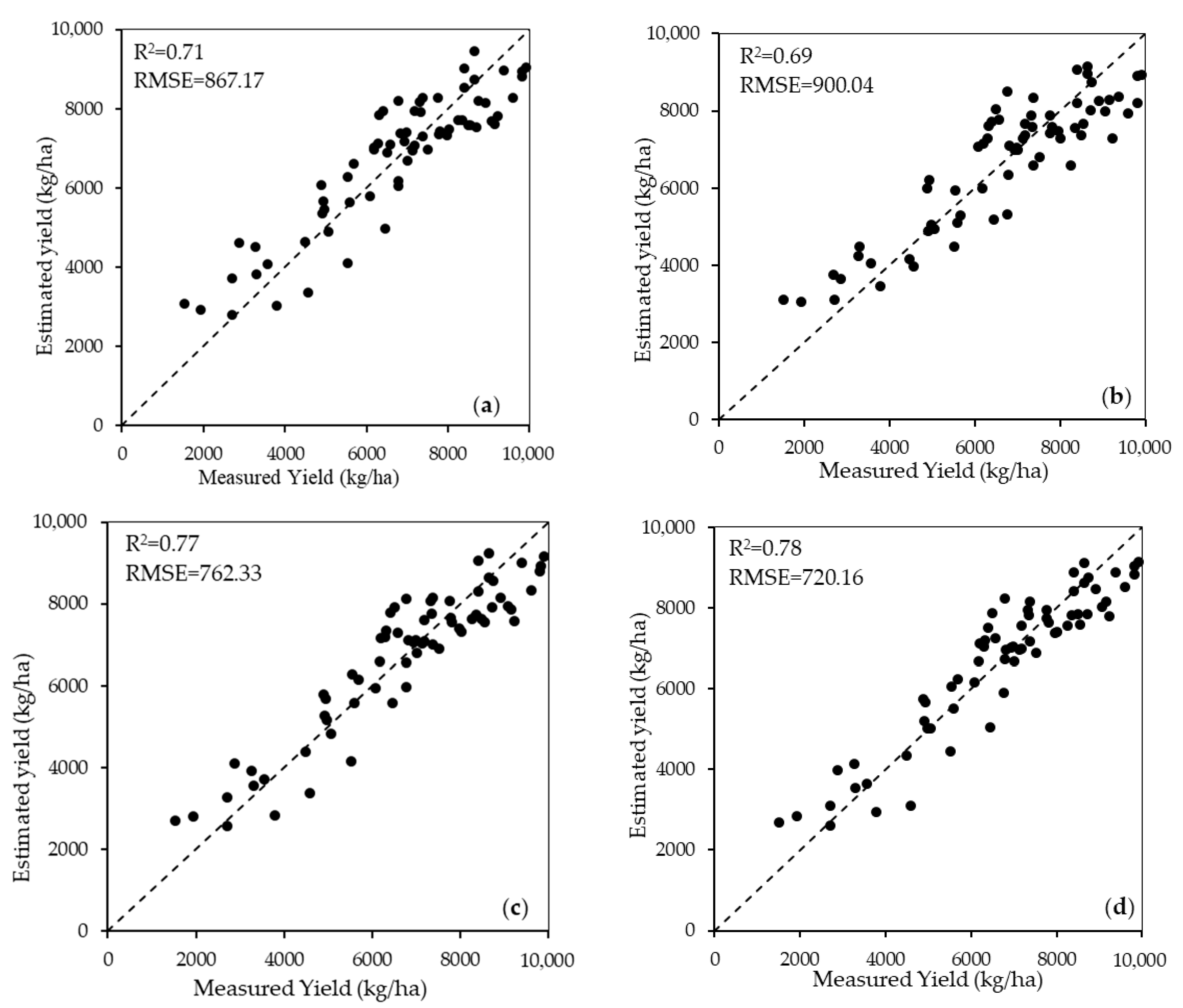
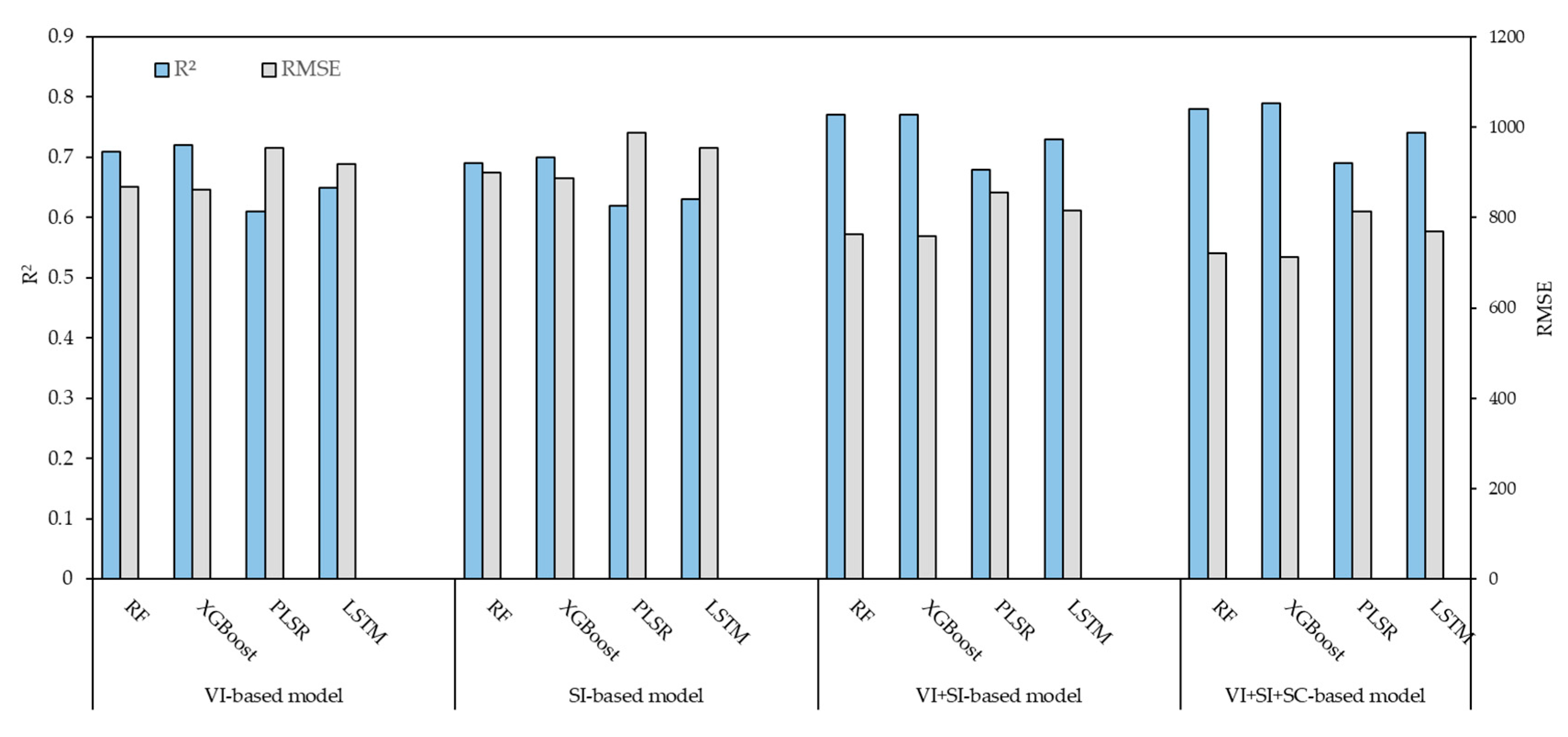
3.2. Winter Wheat Yield Estimation Using Random Forest

As shown in Figure 5, single temporal remote sensing parameter-based wheat yield estimation modeling revealed period-dependent performance: the VI-based group model achieved optimal results during P5 (R² = 0.64, RMSE = 1268.2 kg/ha), while the SI-based model performed better in P6 (R² = 0.56, RMSE = 1465.6 kg/ha). Notably, the VI + SI-based model demonstrated promising performance in P5 (R² = 0.65, RMSE = 1214.5 kg/ha).

To enhance yield estimation accuracy across growth periods, we employed a progressive time-step approach (P1, P1–P2, P1–P3, P1–P4, P1–P5, P1–P6) to investigate information contribution. Using the random forest regression method, we analyzed VI-, SI-, and VI + SI-based group models and compared R² and RMSE. The results demonstrated the consistent superiority of VI + SI-based models over single-index methods in all periods.

The R² values of different groups exhibited the order of VI + SI > SI > VI during pre-jointing growth periods (P1–P3). Compared to R² of P1, R² of integrated P1–P2 increased from 0.12 to 0.27 for the VI-based model, 0.15 to 0.37 for the SI-based model, and reached 0.43 for the VI + SI-based model. For P3, R² of the VI + SI-based model achieved 0.55, demonstrating a 22.53% accuracy advantage over the VI-based model. R² exhibited a hierarchy of VI + SI > VI > SI due to increased vegetation coverage during post-jointing growth periods. R² of the VI + SI-based model maintained substantial improvements: 14.33% and 18.81% higher values than VI and SI across P1–P4, respectively, with an R² of 0.75 (VI + SI-based model) versus 0.71 (VI-based model) and 0.65 (SI-based model) at P1–P5. Across the complete growth periods (P1–P6), the R² (0.77) and RMSE (762.33 kg/ha) of the VI + SI-based model demonstrated consistent improvements over those of the VI-based model (R² = 0.71, RMSE = 867.17 kg/ha) and SI-based model (R² = 0.69, RMSE = 900.04 kg/ha), with R² gains of 8.45% and 11.59%, respectively.

The model in the VI + SI-based group achieved a good performance across the P1–P6 periods. To further enhance accuracy, we integrated field-measured soil salt content (SC) data to establish a VI + SI + SC-based composite model. As illustrated in Figure 6d, the integration of field soil parameters improved the estimative capability, and the R² and RMSE in the VI + SI + SC-based model were 0.78 and 720.16 kg/ha, respectively. Compared with VI-based, SI-based, and VI + SI-based models, the R² in VI + SI + SC-based group increased by 9.86%, 13.04%, and 1.30%, respectively.

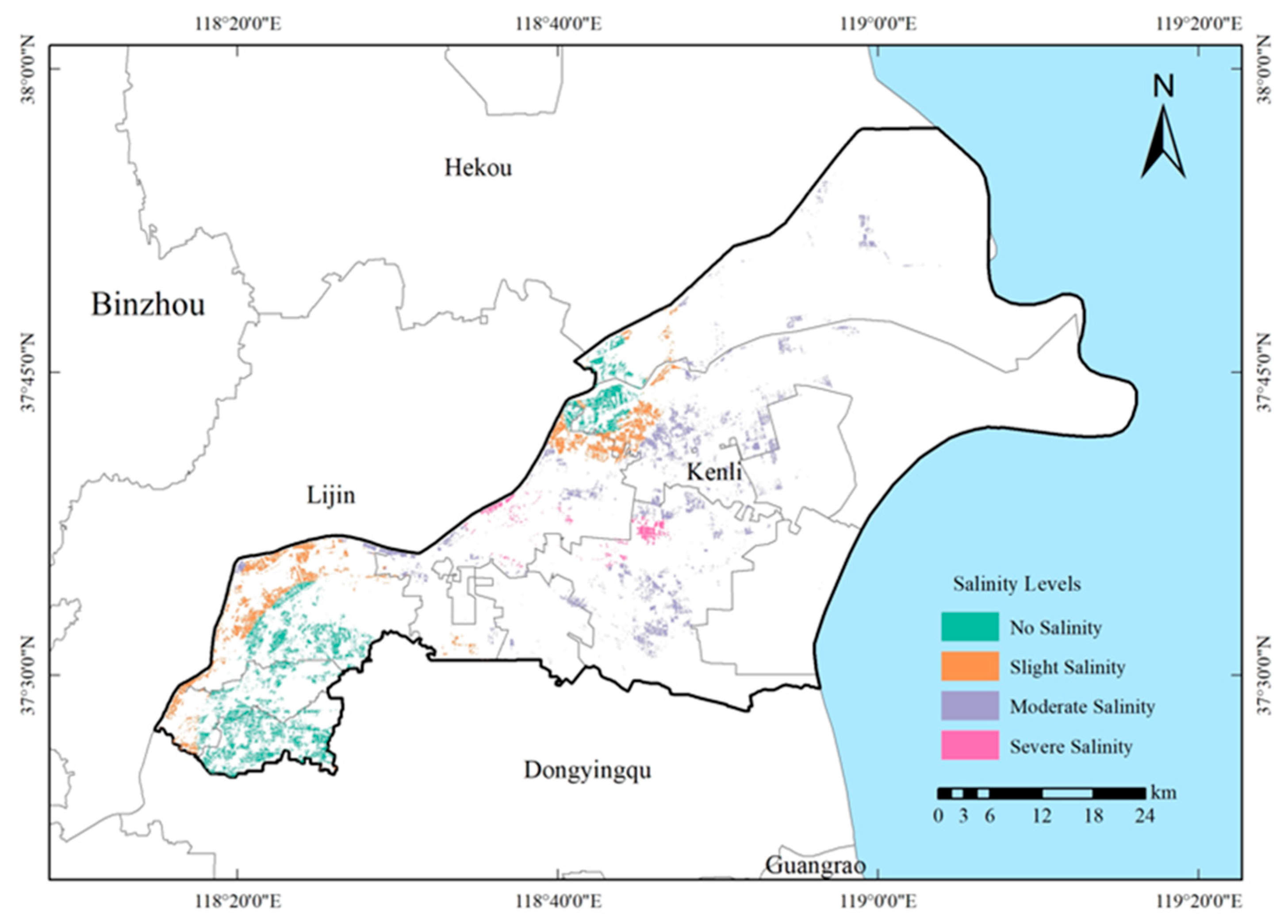
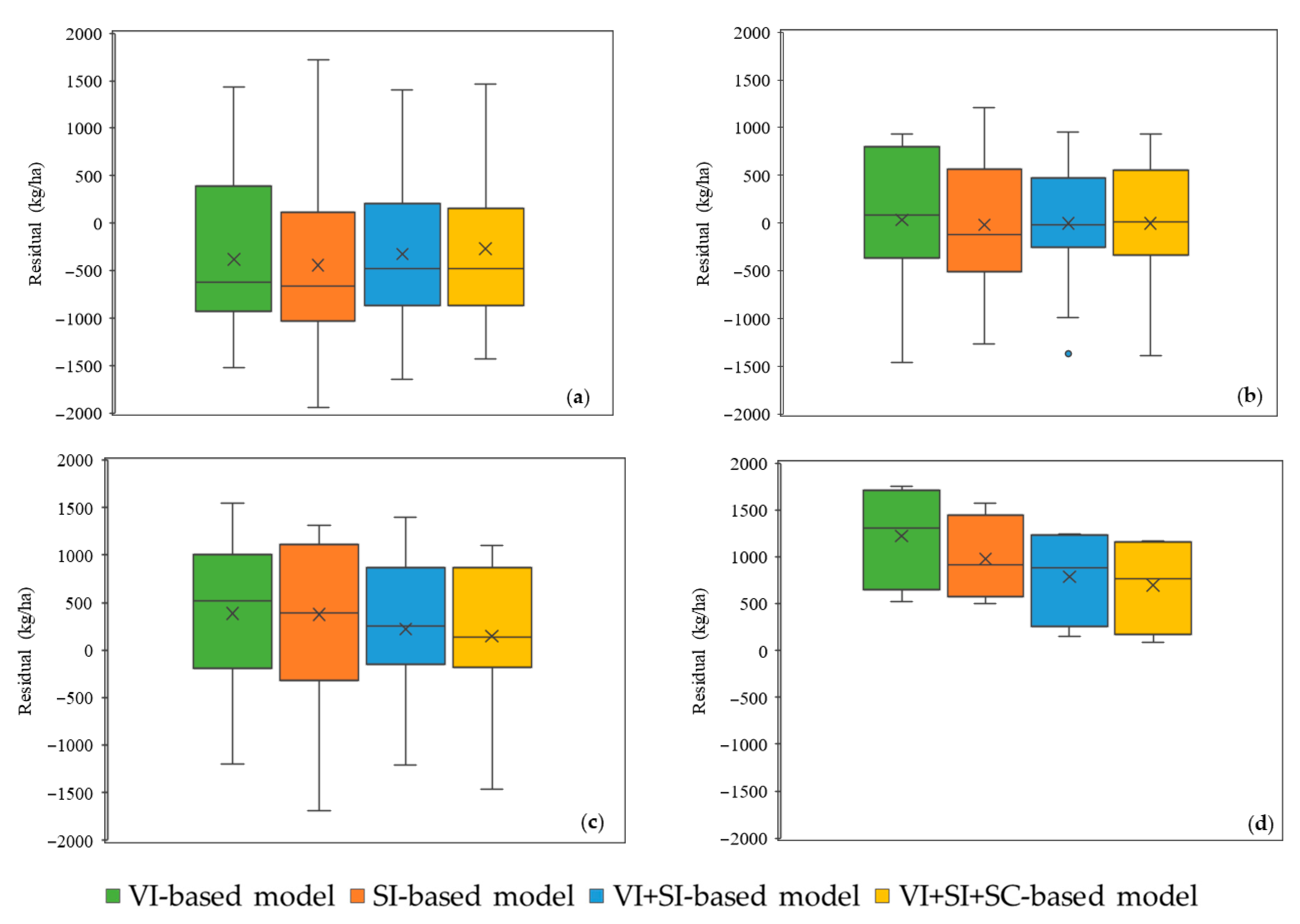
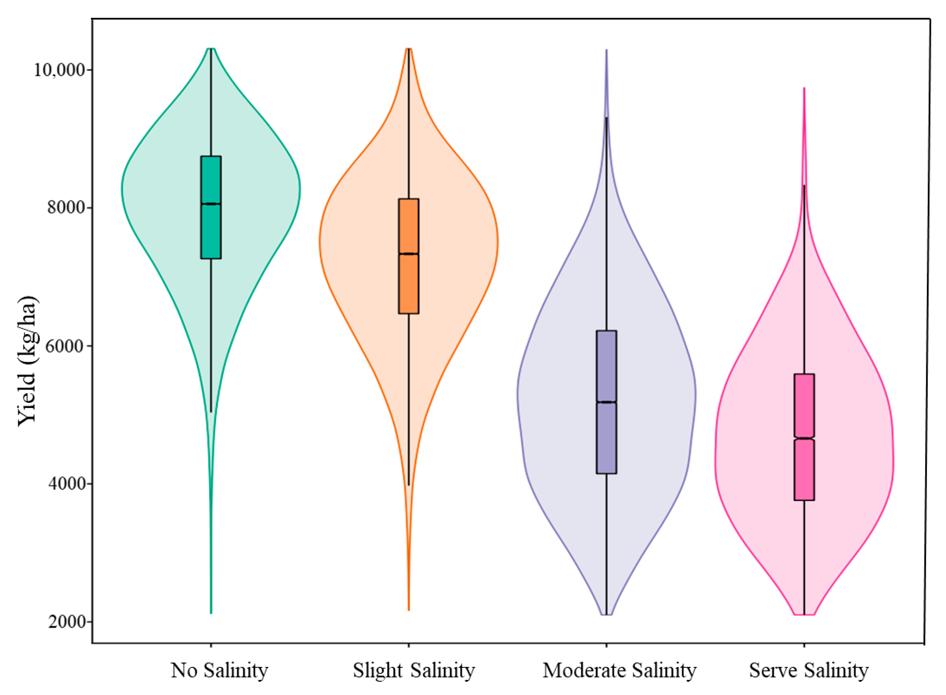
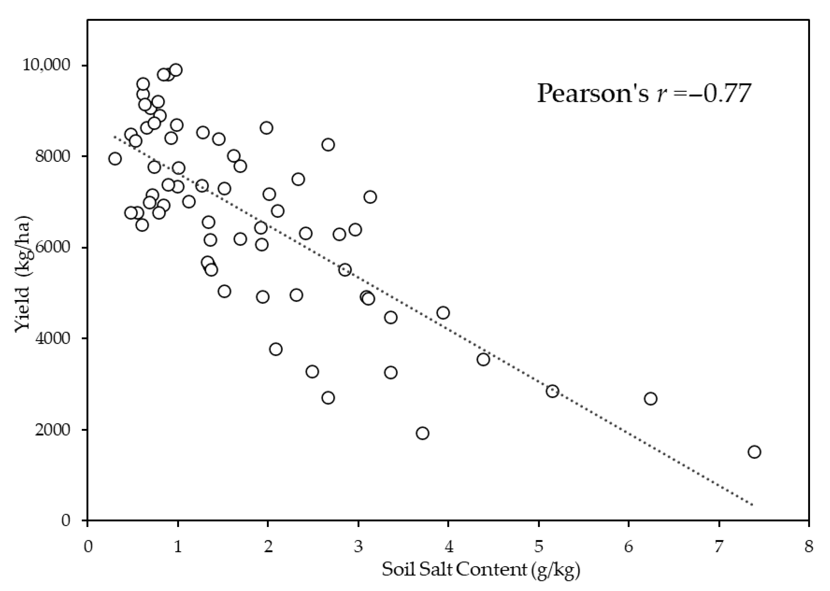
3.3. Estimation Error Under Different Salinity Levels

We analyzed the residuals of estimated and field-measured yields at different salinity levels (Table 1) to evaluate model generalization across salinity gradients, as shown in Figure 7. Positive residuals indicated overestimation, while negative values suggested underestimation. In general, the results in slight salinity demonstrated optimal performance (mean residual under all groups: 0.42 kg/ha), and the yields in moderate and severe salinity were overestimated (corresponding mean residual: 281.65, 920.84 kg/ha, respectively).

Detailed model performance analysis showed variations across salinity gradients. At the no salinity level, compared to VI-based and SI-based models, the VI + SI-based model reduced estimation errors, and the residual ranged from −1651.08 to 1405.48 kg/ha. The VI + SI + SC-based model exhibited a residual with a value of −1429.79 to 1466.41 kg/ha, which maintained a relatively lower mean residual. For the slight salinity level, both VI + SI-based and VI + SI + SC-based models exhibited tighter residual distributions for better capturing yield variations. At the moderate salinity level, the estimated accuracy improved progressively with model complexity, as shown by decreasing mean residuals from 385.09 kg/ha (VI-based model) and 373.36 kg/ha (SI-based model) to 220.83 kg/ha (VI + SI-based model) and finally 147.30 kg/ha (VI + SI + SC-based model). At the severe salinity level, the mean residual of VI + SI + SC-based model was 696.01 kg/ha, representing reductions of 43.01%, 28.77%, and 11.77% compared with VI-based, SI-based, and VI + SI based models.

The comprehensive analysis results demonstrated that the VI + SI + SC-based model showed distinct advantages in feature extraction across high salinity gradients and effectively integrated crop and soil factors to achieve more accurate yield estimation.

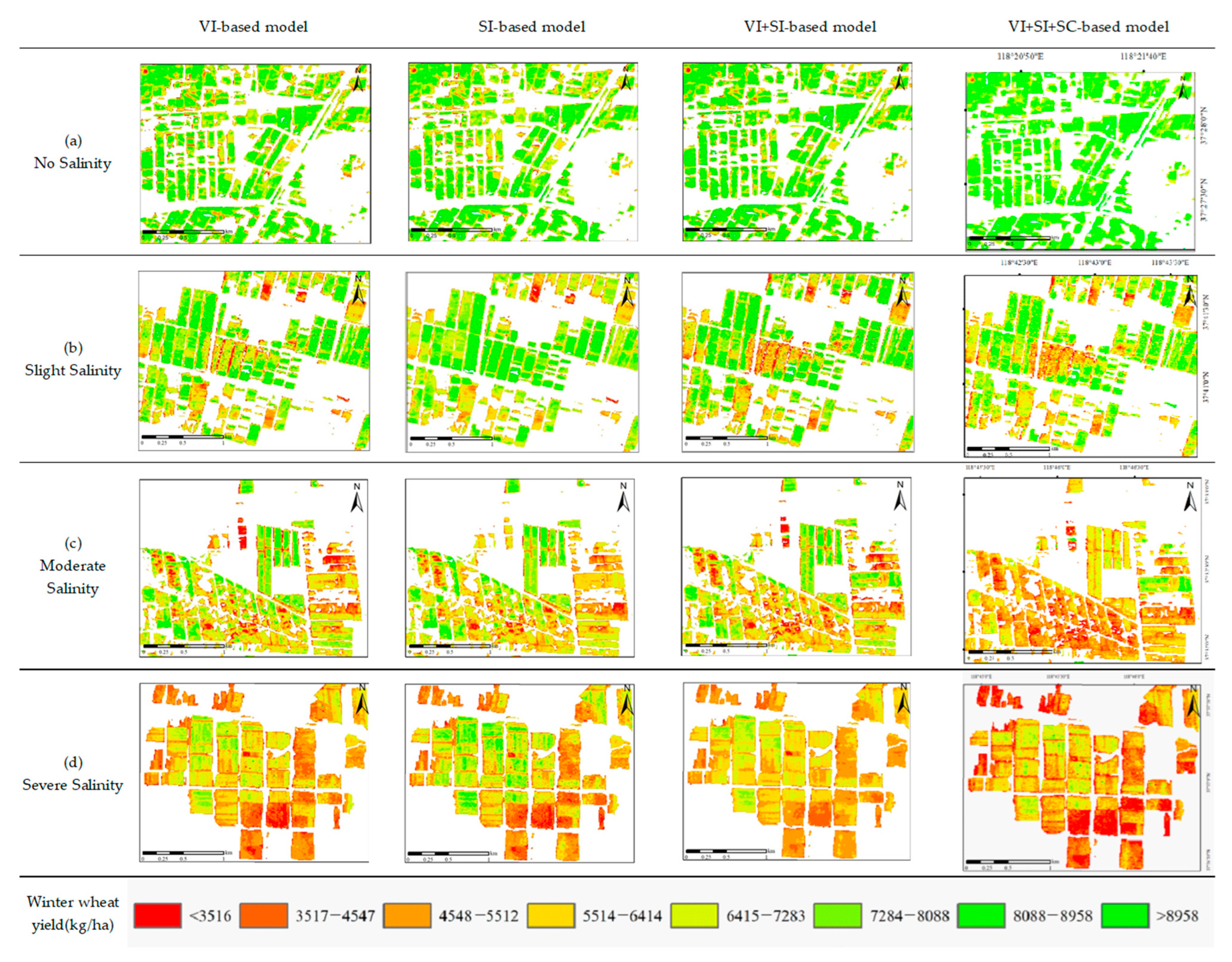
3.4. Winter Wheat Yield Mapping and Feature Analysis

Based on the previous analysis and results, we employed the VI + SI + SC-based model using random forest to generate a county-level yield map of winter wheat by integrating its spatial distribution data, as shown in Figure 8. The estimated wheat yield ranged from 2100 to 10,310 kg/ha (mean = 6771 kg/ha), which was consistent with the statistical data from the Kenli government during the same period.

Winter wheat yield maps using VI-based, SI-based, and VI + SI-based models were also produced, and yield map comparisons of the subsets are presented in Figure 9. In no salinity areas, all models showed minor spatial variation of winter wheat yield. In saline-affected regions, the VI-based model demonstrated limited sensitivity to salinity-induced yield changes, while the VI + SI-based and VI + SI + SC-based models effectively captured critical yield-related information using multi-parameter integration and time-series analysis to outperform single-parameter models.

Compared with the soil salinity interpolation results in Figure 2, the spatial distribution of winter wheat yield in Figure 8 strongly correlated with soil salinity levels. High yields were concentrated in western regions, and low yields clustered in the central and eastern areas. According to the violin plot of the yield data distribution shown in Figure 10, the average yield in the no salinity areas mainly distributed in southwest and north was 7945 kg/ha, and most yields fell within the range of 7200–8800 kg/ha. Slight saline areas were predominantly distributed along the Yellow River in the western region, with an average yield of 7258 kg/ha. Moderate and severe saline areas in central regions showed reduced yields of 5217 kg/ha and 4707 kg/ha, respectively.

4. Discussion

4.1. Importance Analysis of Parameters in Each Period

Feature selection for input parameters of yield models is very important due to significant improvements in model accuracy and computational efficiency [36,37]. Given the dynamic accumulation process of wheat growth and its varied tolerance to seasonal soil salinity fluctuations, which are characterized by spring salt accumulation, summer leaching desalination, autumn re-accumulation via evaporation, and winter stabilization [38], in this study, period-specific feature selection of remote sensing parameters for winter wheat were implemented. This process qualitatively identifies key feature factors and quantitatively analyzes parameter importance for yield estimation. During early growth periods (seedling—dormancy), VI demonstrated relatively weak predictive performance due to insufficient dry matter accumulation. Conversely, multiple SI demonstrated higher predictive importance due to wheat’s heightened sensitivity to saline stress during initial growth phases [39]. However, early-period soil feature extraction may be influenced by tillage practices, potentially causing instability of individual estimative features. To address this, multiple indexes (SI1, SI3, and SI4) were integrated to enhance the stability and reliability of parameter–soil salinity correlations. During the jointing period, when wheat experiences peak water demand and concurrent topsoil salt accumulation, canopy moisture indexes (NDWI and NDMI) exhibited better yield prediction performance. This enhancement may be attributed to their capacity to monitor irrigation-driven water availability under saline stress, a critical factor for final yield formation [40,41]. In addition, chlorophyll parameters (CARI and CCRI) showed increased estimative importance due to their sensitivity to salinity-induced chlorophyll degradation [42]. The booting-flowering period, when spike number per unit area is determined and leaf area stabilizes, showed the highest predictive utility of vegetation indexes (NDVI, EVI, NDMI, NDWI, CARI). This critical phase affects final grain weight and spike fertility, explaining the high accuracy regression models, which were consistent with established physiological principles [43,44]. During grain filling, although chlorophyll degradation and leaf senescence reduce VI predictive capacity, data integration remains essential due to salinity’s potential impact on dry matter partitioning. Notably, post-vegetative growth period analysis revealed weaker yield correlations for SI1 and SI4, while CRSI maintained stronger correlations. By analyzing vegetation canopy spectral responses to salt stress, CRSI effectively integrates vegetation indexes and soil salinity characteristics, accurately reflecting the impacts of soil salinity on vegetation growth [45].

4.2. Comparisons of Different Parameter Combinations

Saline stress impairs yield formation through multiple mechanisms: inhibiting leaf expansion, weakening chlorophyll synthesis, accelerating foliar water loss, and restraining grain filling [46]. While vegetation indexes (e.g., NDVI, CARI) effectively characterize canopy structure and growth status, their utility is limited under saline conditions due to reduced dry matter allocation to reproductive growth [47,48], potentially leading to yield estimation inaccuracies. The VI + SI + SC-based model developed in this study enhanced yield estimation accuracy across varying salinity levels. The model’s effectiveness stems from two key aspects. On the one hand, soil salt content data, which demonstrated a strong negative correlation with yield (r = −0.77, Figure 11), were incorporated. This integration improved physiological state representation, reducing estimation errors in moderate-to-severe salinity levels. Similar benefits were observed in Lebrija’s saline farmland, where combining soil electrical conductivity with NDVI imagery enhanced spatial assessment of crop growth impacts during tomato–cotton–sugar rotation seasons [49]. On the other hand, salinity index integration provided crucial soil salinity information, particularly during low vegetation cover periods when VI was weak. This complement effectively addressed early growth period monitoring limitations under saline stress, corroborating findings from Karimli’s high-precision wheat yield estimation in Jalilabad [12] and Li et al.’s successful soil salinity inversion [28]. Notably, the integration of SC into the VI + SI-based model resulted in only marginal improvement (R² increasing from 0.77 to 0.78), which may be explained by the following factors including the temporal mismatch between soil salinity sampling and crop growth dynamics, compensatory effects between SC and SI, and spatial resolution limitations inherent in the 10 km² interpolation approach. Despite these limitations, the inclusion of SC provided essential soil constraints that significantly reduced model residuals under our experimental conditions. For other soil types exhibiting lower risk thresholds [50], the model’s performance improvement with SC incorporation may be more pronounced. From a practical standpoint, soil data integration offers valuable yield estimation corrections, especially for smaller study areas where such data are readily available. However, extensive sampling and mapping requirements make this approach impractical for larger regions. In such cases, the VI + SI-based model demonstrates reasonable estimation capability through mutual complementarity.

Model validation revealed that in saline-affected areas, poor canopy structure indicated by low VI values led to overestimation. The integrated model effectively captured yield variations across salinity gradients, enabling accurate yield mapping. Regional analysis showed progressive yield reductions of 8.65%, 34.33%, and 40.76% in slight, moderate, and severe saline areas compared to no salinity conditions, highlighting wheat’s limited tolerance to moderate and severe saline stress. The results had practical significance for both operational forecasting and precision management. The model’s ability to achieve moderate early-season accuracy (Figure 5) at 10 m resolution enables timely identification of salinity stress hotspots before irreversible yield loss occurs. Farmers could leverage this for targeted irrigation scheduling at the field scale. The spatial yield-salinity deviation maps (Figure 8 and Figure 9) facilitate zone-specific interventions. Severe salinity zones (SC > 4 g/kg, and yield <4707 kg/ha) may require land rehabilitation, subsurface drainage, or alternative crops to mitigate high-salinity stress risks. Moderate salinity zones will benefit from soil amendments such as gypsum or organic matter, while slight salinity zones can adopt preventive measures like salt-tolerant cultivars. For policymakers, the results offer a scalable framework to monitor salinity’s impact on productivity as part of strategies for safeguarding food security, aligning with China’s ‘Saline Soil Utilization’ policy.

4.3. Uncertainty Analysis

As shown in Figure 12, a comparison experiment demonstrates that RF and XGBoost consistently outperformed other methods across all combinations (VI-based model, SI-based model, VI + SI-based model, and VI + SI + SC-based model; P1~P6 cumulative periods). For the VI + SI + SC-based model, both RF and XGBoost algorithms achieved superior performance with R² values of 0.78 and 0.79 and RMSE values of 720.16 and 712.89 kg/ha, respectively, significantly surpassing PLSR (R² = 0.69) and LSTM (R² = 0.74). In the VI + SI-based model, RF achieved comparable performance to XGBoost (R² = 0.77). Although XGBoost exhibited marginally higher accuracy, RF was selected based on comprehensive evaluation of prediction stability, computational efficiency, and model explainability. Moreover, given our limited sample size (n = 68), RF’s inherent mechanisms including out-of-bag error estimation and bootstrap aggregation provide robust performance validation and prevent overfitting, as evidenced by previous studies using small datasets [51]. In comparative experiments of various yield estimation modeling approaches, RF demonstrated superior stability [32,52,53]. However, the model was developed and validated using data from a single growing season. Given the interannual variations in precipitation, soil salinity, and management, its applicability to other years may be limited. Future studies should incorporate multi-year datasets to enhance validation reliability and address potential uncertainties in the algorithm’s extrapolation performance across broader agricultural contexts.

Data sources used in this study have two primary limitations. First, the even sampling density across heterogeneous salinity distributions resulted in imbalanced sample representativeness, particularly with limited data from severe salinity areas to potentially affect estimation accuracy. Second, soil salt content data measured in the harvest period provide general plot-level salinity characterization, representing relationships between parameters at different periods (Figure 13), but they cannot fully capture the dynamic salinity variations. These limitations highlight the need for further validation of temporal relationships among soil salt content, salinity indexes, and crop yield using comprehensive multi-source datasets. In digital soil salinity mapping, future research would benefit from incorporating regression Kriging or co-Kriging methodologies.

Regarding regional specificity, the model was developed based on loam and sandy loam textured soils and did not incorporate different soil texture parameters. These parameters are known to affect salinity tolerance through their influence on soil structure, porosity, and hydraulic properties [54]. This texture-specific development may constrain the model’s transferability to other saline regions with distinct soil matrices. Future studies will integrate water and salt transport characteristics across varying soil textures and implement stress risk calibration. Furthermore, while the winter wheat distribution map demonstrated good accuracy, it must be acknowledged that classification uncertainty may propagate to the yield estimation. The robustness of our yield model (R² = 0.78) and the leave-one-out cross-validation approach likely helped mitigate some classification-related uncertainties. Residual analysis showed no strong systematic patterns attributable to classification errors, although we cannot completely rule out some localized effects. We will further discuss these limitations and suggest methods to reduce uncertainties in future studies.

5. Conclusions

This study investigated winter wheat yield estimation in salinity areas of Kenli County, Yellow River Delta, China, by developing random forest regression models incorporating vegetation indexes, salinity indexes derived from Sentinel-2 images, and surface soil salt content. The results and findings are outlined as follows:

(1) The dominant yield estimation parameters varied across growth periods. SI (SI1, SI2, SI3) had higher feature importance in pre-jointing periods, while VI (e.g., NDMI) demonstrated greater estimative importance for winter wheat yield in post-jointing periods.

(2) The combined VI + SI-based method within the RF framework demonstrated a good wheat yield estimation performance during the wheat flowering stage among single-temporal analyses (R² = 0.65, RMSE = 1214.5 kg/ha). In the cumulative period, the VI + SI-based model (R² = 0.77, RMSE = 762.33 kg/ha) significantly outperformed individual VI-based or SI-based models, and its R² correspondingly improved by 8.45% and 11.59%, respectively. The VI + SI + SC-based model achieved the optimal estimation accuracy, and the R² improved by 9.86%, 13.04%, and 1.30% compared to VI-based, SI-based, and VI + SI-based models, respectively.

(3) Salinity stress affected yield estimation accuracy. The incorporation of SI and SC data played a crucial role in error reduction. At the moderate salinity level, mean residuals decreased from 385.09 kg/ha (VI-based) to 220.83 kg/ha (VI + SI-based) and 147.30 kg/ha (VI + SI + SC-based). At the severe salinity level, although all models exhibited overestimation, the VI + SI + SC-based model showed the closest approximation to measured yields (mean residual = 696.01 kg/ha), representing a 43.01% reduction versus the VI-based model.

The results demonstrated the effectiveness of multi-source parameters for accurate estimation of winter wheat yield across no salinity (7945 kg/ha), slight (7258 kg/ha), moderate (5217 kg/ha), and severe (4707 kg/ha) salinity areas in 2024, providing a critical reference for refining planting strategies and decision making. Future research should develop alternative regression algorithms and incorporate dynamic soil salinity data to further enhance estimation accuracy.

References

1. Guo, B.; Liu, Y.; Fan, J.; Lu, M.; Zang, W.; Liu, C.; Wang, B.; Huang, X.; Lai, J.; Wu, H. The salinization process and its response to the combined processes of climate change–human activity in the Yellow River Delta between 1984 and 2022. Catena 2023, 231, 107301. [Google Scholar] [CrossRef]
2. Chen, X.; Huang, Q.; Xiong, Y.; Yang, Q.; Li, H.; Hou, Z.; Huang, G. Tracking the spatio-temporal change of the main food crop planting structure in the Yellow River Basin over 2001–2020. Comput. Electron. Agr. 2023, 212, 108102. [Google Scholar] [CrossRef]
3. Su, W.; Magdziarczyk, M.; Smolinski, A. Increasing overall agricultural productivity in the Yellow River Delta Eco-economic Zone in China. Reg. Environ. Change 2024, 24, 64. [Google Scholar] [CrossRef]
4. Zhu, W.; Li, S.; Zhang, X.; Li, Y.; Sun, Z. Estimation of winter wheat yield using optimal vegetation indices from unmanned aerial vehicle remote sensing. Trans. Chin. Soc. Agric. Eng. 2018, 34, 78–86. [Google Scholar]
5. Satir, O.; Berberoglu, S. Crop yield prediction under soil salinity using satellite derived vegetation indices. Field Crops Res. 2016, 192, 134–143. [Google Scholar] [CrossRef]
6. Shi, F.; Wang, R.; Li, Y.; Yan, H.; Zhang, X. LAI estimation based on multi-spectral remote sensing of UAV and its application in saline soil improvement. Sci. Agric. Sin. 2020, 53, 1795–1805. [Google Scholar]
7. Chen, Y.; Zhao, G.; Chang, C.; Wang, Z.; Li, Y.; Zhao, H.; Pan, J. Grain yield estimation of wheat-maize rotation cultivated land based on Sentinel-2 multi-spectral image: A case study in Caoxian County, Shandong, China. Chin. J. Appl. Ecol. 2023, 34, 3347–3356. [Google Scholar]
8. Zhao, L.; Hua, L.; Hui, C.; Zhang, S. Maize yield forecasting and associated optimum lead time research based on temporal remote sensing data and different model. Spectrosc. Spect. Anal. 2023, 43, 2627–2637. [Google Scholar]
9. Abbas, F.; Afzaal, H.; Farooque, A.A.; Tang, S. Crop yield prediction through proximal sensing and machine learning algorithms. Agronomy 2020, 10, 1046. [Google Scholar] [CrossRef]
10. Han, J.; Zhang, Z.; Cao, J.; Luo, Y.; Zhang, L.; Li, Z.; Zhang, J. Prediction of winter wheat yield based on multi-source data and machine learning in China. Remote Sens. 2020, 12, 236. [Google Scholar] [CrossRef]
11. Mustafa, G.; Moazzam, M.A.; Nawaz, A.; Ali, T.; Alsekait, D.M.; Alattas, A.S.; AbdElminaam, D.S. ECP-IEM: Enhancing seasonal crop productivity with deep integrated models. PLoS ONE 2025, 20, e316682. [Google Scholar]
12. Karimli, N.; Selbesoğlu, M.O. Remote sensing-based yield estimation of winter wheat using vegetation and soil indices in Jalilabad, Azerbaijan. ISPRS. Int. J. Geo-Inf. 2023, 12, 124. [Google Scholar] [CrossRef]
13. Mahboob, W.; Rizwan, M.; Irfan, M.; Hafeez, O.B.A.; Sarwar, N.; Akhtar, M.; Munir, M.; Rani, R. Salinity tolerance in wheat: Responses, mechanisms and adaptation approaches. Appl. Ecol. Env. Res. 2023, 21, 5299–5328. [Google Scholar] [CrossRef]
14. Wang, W.; Zou, J.; Zhang, Y.; Niu, L.; Yu, L.; Wang, Z.; Wang, F.; Zhang, S.; Yang, X. Salinity stress phenotyping of wheat germplasm under multiple growth conditions and transcriptomic analysis of two wheat varieties contrasting in their salinity stress tolerance. Plant Growth Regul. 2025, 105, 739–757. [Google Scholar] [CrossRef]
15. Zhang, Z.; Fan, Y.; Zhang, A.; Jiao, Z. Baseline-Based Soil Salinity Index (BSSI): A novel remote sensing monitoring method of soil salinization. IEEE J. Stars. 2023, 16, 202. [Google Scholar] [CrossRef]
16. Aboelsoud, H.M.; AbdelRahman, M.A.E.; Kheir, A.M.S.; Eid, M.S.M.; Ammar, K.A.; Khalifa, T.H.; Scopa, A. Quantitative estimation of saline-soil amelioration using remote-sensing indices in arid land for better management. Land 2022, 11, 1041. [Google Scholar] [CrossRef]
17. Cui, X.; Han, W.; Zhang, H.; Dong, Y.; Ma, W.; Zhai, X.; Zhang, L.; Li, G. Estimating and mapping the dynamics of soil salinity under different crop types using Sentinel-2 satellite imagery. Geoderma 2023, 440, 116738. [Google Scholar] [CrossRef]
18. Liu, X.; Hu, Y.; Zhang, S.; Bai, Y.; Zhang, H. Comparison of different salinity estimation models for salinized soils on south bank of Yellow River in Dalat Banner. Trans. Chin. Soc. Agric. Mach. 2024, 55, 360–370. [Google Scholar]
19. Wang, J.; Ding, J.; Ge, X.; Peng, J.; Hu, Z. Monitoring soil salinization on the basis of remote sensing and proximal soil sensing: Progress and perspective. Nat. Remote Sens. Bull. 2024, 28, 2187–2208. [Google Scholar]
20. Zhang, X.; Wang, Z.; Song, X.; Liu, P.; Li, S.; Yang, X. Effect of sampling on spatial variability in soil salinity in the Yellow River Delta Area. Resour. Sci. 2016, 38, 2375–2382. [Google Scholar]
21. Zhang, Z.; Song, Y.; Zhang, H.; Li, X.; Niu, B. Spatiotemporal dynamics of soil salinity in the Yellow River Delta under the impacts of hydrology and climate. Chin. J. Appl. Ecol. 2021, 32, 1393–1405. [Google Scholar]
22. Technical Regulations and Specifications for the Third National Soil Census (Revised Edition). Available online: http://www.moa.gov.cn/ztzl/dscqgtrpc/zywj/202307/t20230720_6432535.htm (accessed on 7 July 2023).
23. Yu, F.; Bai, J.; Fang, J.; Guo, S.; Zhu, S.; Xu, T. Integration of a parameter combination discriminator improves the accuracy of chlorophyll inversion from spectral imaging of rice. Agric. Commun. 2024, 2, 100055. [Google Scholar] [CrossRef]
24. Sellami, M.H.; Albrizio, R.; Čolović, M.; Hamze, M.; Cantore, V.; Todorovic, M.; Piscitelli, L.; Stellacci, A.M. Selection of hyperspectral vegetation indices for monitoring yield and physiological response in sweet maize under different water and nitrogen availability. Agronomy 2022, 12, 489. [Google Scholar] [CrossRef]
25. Gitelson, A.; Merzlyak, M. Remote estimation of chlorophyll content in higher plant leaves. Int. J. Remote Sens. 1997, 18, 2691–2697. [Google Scholar] [CrossRef]
26. Solgi, S.; Ahmadi, S.H.; Seidel, S.J. Remote sensing of canopy water status of the irrigated winter wheat fields and the paired anomaly analyses on the spectral vegetation indices and grain yields. Agric. Water Manag. 2023, 280, 108226. [Google Scholar] [CrossRef]
27. Jin, X.; Kumar, L.; Li, Z.; Xu, X.; Yang, G.; Wang, J. Estimation of winter wheat biomass and yield by combining the AquaCrop model and field hyperspectral data. Remote Sens. 2016, 8, 972. [Google Scholar] [CrossRef]
28. Li, Y.; Chang, C.; Wang, Z.; Zhao, G. Remote sensing prediction and characteristic analysis of cultivated land salinization in different seasons and multiple soil layers in the coastal area. Int. J. Appl. Earth Obs. 2022, 111, 102838. [Google Scholar] [CrossRef]
29. Scudiero, E.; Skaggs, T.H.; Corwin, D.L. Regional scale soil salinity evaluation using Landsat 7, western San Joaquin Valley, California, USA. Geoderma Reg. 2014, 2, 82–90. [Google Scholar] [CrossRef]
30. Zhou, K.; Liu, L.; Zhang, Y.; Miao, R.; Yang, Y. Area Extraction and growth monitoring of winter wheat in Henan province supported by Google Earth Engine. Sci. Agric. Sin. 2021, 54, 2302–2318. [Google Scholar]
31. Zhang, D.; Ying, C.; Wu, L.; Meng, Z.; Wang, X.; Ma, Y. Using time series sentinel images for object-oriented crop extraction of planting structure in the Google Earth Engine. Agronomy 2023, 13, 2350. [Google Scholar] [CrossRef]
32. Jabed, M.A.; Azmi Murad, M.A. Crop yield prediction in agriculture: A comprehensive review of machine learning and deep learning approaches, with insights for future research and sustainability. Heliyon 2024, 10, e40836. [Google Scholar] [CrossRef] [PubMed]
33. Feng, H.; Fan, Y.; Yue, J.; Ma, Y.; Liu, Y.; Chen, R.; Fu, Y.; Jin, X.; Bian, M.; Fan, J.; et al. Enhancing potato leaf protein content, carbon-based constituents, and leaf area index monitoring using radiative transfer model and deep learning. Eur. J. Agron. 2025, 166, 127580. [Google Scholar] [CrossRef]
34. Wang, Y.; Chen, H.; Chen, J.; Wang, H.; Xing, Z.; Zhang, Z. Comparation of rice yield estimation model combining spectral index screening method and statistical regression algorithm. Trans. Chin. Soc. Agric. Eng. 2021, 37, 208–216. [Google Scholar]
35. Qader, S.H.; Dash, J.; Atkinson, P.M. Forecasting wheat and barley crop production in arid and semi-arid regions using remotely sensed primary productivity and crop phenology: A case study in Iraq. Sci. Total Environ. 2018, 613, 250–262. [Google Scholar] [CrossRef] [PubMed]
36. Fan, Y.; Liu, Y.; Yue, J.; Jin, X.; Chen, R.; Bian, M.; Ma, Y.; Yang, G.; Feng, H. Estimation of potato yield using a semi-mechanistic model developed by proximal remote sensing and environmental variables. Comput. Electron. Agr. 2024, 223, 109117. [Google Scholar] [CrossRef]
37. Li, Z.; Zhou, X.; Cheng, Q.; Zhai, W.; Mao, B.; Li, Y.; Chen, Z. An integrated feature selection approach to high water stress yield prediction. Front. Plant Sci. 2023, 14, 1289692. [Google Scholar] [CrossRef] [PubMed]
38. Fu, T. The Temporal and Spatial Variation of Soil Salinization in Typical Coastal Area and Application Research of the Monitoring System. Ph.D. Thesis, Chinese Academy of Sciences, Beijing, China, 2015. [Google Scholar]
39. Saddiq, M.S.; Iqbal, S.; Hafeez, M.B.; Ibrahim, A.M.H.; Raza, A.; Fatima, E.M.; Baloch, H.; Jahanzaib; Woodrow, P.; Ciarmiello, L.F. Effect of Salinity stress on physiological changes in winter and spring wheat. Agronomy 2021, 11, 1193. [Google Scholar] [CrossRef]
40. Yue, J.; Li, T.; Feng, H.; Fu, Y.; Liu, Y.; Tian, J.; Yang, H.; Yang, G. Enhancing field soil moisture content monitoring using laboratory-based soil spectral measurements and radiative transfer models. Agric. Commun. 2024, 2, 100060. [Google Scholar] [CrossRef]
41. Wang, T.; Xu, Z.; Pang, G. Effects of Irrigating with Brackish Water on soil moisture, soil salinity, and the agronomic response of winter wheat in the Yellow River Delta. Sustainability 2019, 11, 5801. [Google Scholar] [CrossRef]
42. Shah, S.; Houborg, R.; McCabe, M. Response of Chlorophyll, Carotenoid and SPAD-502 measurement to salinity and nutrient stress in wheat (Triticum aestivum L.). Agronomy 2017, 7, 61. [Google Scholar] [CrossRef]
43. Cai, Y.; Guan, K.; Lobell, D.; Potgieter, A.B.; Wang, S.; Peng, J.; Xu, T.; Asseng, S.; Zhang, Y.; You, L.; et al. Integrating satellite and climate data to predict wheat yield in Australia using machine learning approaches. Agr. Forest Meteorol. 2019, 274, 144–159. [Google Scholar] [CrossRef]
44. Li, Y.; Zhao, B.; Wang, J.; Li, Y.; Yuan, Y. Winter wheat yield estimation based on multi-temporal and multi-sensor remote sensing data fusion. Agriculture 2023, 13, 2190. [Google Scholar] [CrossRef]
45. Wang, D.; Yang, H.; Qian, H.; Gao, L.; Li, C.; Xin, J.; Tan, Y.; Wang, Y.; Li, Z. Minimizing vegetation influence on soil salinity mapping with novel bare soil pixels from multi-temporal images. Geoderma 2023, 439, 116697. [Google Scholar] [CrossRef]
46. Rani, S.; Sharma, M.K.; Kumar, N.; Neelam. Impact of salinity and Zinc application on growth, physiological and yield traits in wheat. Curr. Sci. 2019, 116, 1324–1330. [Google Scholar] [CrossRef]
47. Feng, H.; Fan, Y.; Yue, J.; Bian, M.; Liu, Y.; Chen, R.; Ma, Y.; Fan, J.; Yang, G.; Zhao, C. Estimation of potato above-ground biomass based on the VGC-AGB model and deep learning. Comput. Electron. Agr. 2025, 232, 110122. [Google Scholar] [CrossRef]
48. Zhao, L.; Li, F.; Chang, Q. Review on crop type identification and yield forecasting using remote sensing. Trans. Chin. Soc. Agric. Mach. 2023, 54, 1–19. [Google Scholar]
49. Gómez Flores, J.L.; Ramos Rodríguez, M.; González Jiménez, A.; Farzamian, M.; Herencia Galán, J.F.; Salvatierra Bellido, B.; Cermeño Sacristan, P.; Vanderlinden, K. Depth-Specific soil electrical conductivity and NDVI elucidate salinity effects on crop development in reclaimed marsh soils. Remote Sens. 2022, 14, 3389. [Google Scholar] [CrossRef]
50. Dai, X.; Huo, Z.; Wang, H. Simulation for response of crop yield to soil moisture and salinity with artificial neural network. Field Crops. Res. 2011, 121, 441–449. [Google Scholar] [CrossRef]
51. Gómez, D.; Salvador, P.; Sanz, J.; Casanova, J.L. Potato yield prediction using machine learning techniques and sentinel 2 data. Remote Sens. 2019, 11, 1745. [Google Scholar] [CrossRef]
52. Khodjaev, S.; Bobojonov, I.; Kuhn, L.; Glauben, T. Optimizing machine learning models for wheat yield estimation using a comprehensive UAV dataset. Model. Earth Syst. Environ. 2025, 11, 15. [Google Scholar] [CrossRef]
53. Subhashree, S.N.; Marcaida, M.; Sunoj, S.; Kindred, D.R.; Thompson, L.J.; Ketterings, Q.M. Exploring the use of high-resolution satellite images to estimate corn silage yield within field. Remote Sens. 2024, 16, 4081. [Google Scholar] [CrossRef]
54. Zhang, X.; Zuo, Y.; Wang, T.; Han, Q. Salinity effects on soil structure and hydraulic properties: Implications for pedotransfer functions in coastal areas. Land 2024, 13, 2077. [Google Scholar] [CrossRef]
Figure 1. Distribution of winter wheat and sampling sites in the study area. (a) Study area; (b) winter wheat sampling; (c) soil sampling; (d) landscape photos of different salinity levels.
Agriculture 15 01544 g001
Figure 2. Spatial distribution of soil salinity.
Agriculture 15 01544 g002
Figure 3. Flowchart of the winter wheat yield estimation method.
Agriculture 15 01544 g003
Figure 4. The importance of parameters in different growth periods. (P1), seeding-tiller; (P2), dormancy; (P3), regreening; (P4), jointing; (P5), booting-flowering; (P6), filling.
Agriculture 15 01544 g004
Figure 5. R2 (a) and RMSE (b) of different yield estimation models for each single and cumulative growth period. P1, seeding-tiller; P2, dormancy; P3, regreening; P4, jointing; P5, booting-flowering; P6, filling.
Agriculture 15 01544 g005
Figure 6. The R2 and RMSE of winter wheat yield estimations in the VI-based (a), SI-based (b), VI + SI-based (c), VI + SI + SC-based (d) groups.
Agriculture 15 01544 g006
Figure 7. Residual box diagram of different models under no salinity (a), slight salinity (b), moderate salinity (c), and severe salinity (d).
Agriculture 15 01544 g007
Figure 8. Spatial distribution of winter wheat yield using the VI + SI + SC-based model. The subsets (a–d) are used for detailed exhibition in Figure 9.
Agriculture 15 01544 g008
Figure 9. Comparison of winter wheat yield estimation results using different models at different salinity levels located in the subsets in Figure 8.
Agriculture 15 01544 g009
Figure 10. Violin plots of winter wheat yield for different salinity levels.
Agriculture 15 01544 g010
Figure 11. Correlation analysis of winter wheat yield and soil salt content in 2024.
Agriculture 15 01544 g011
Figure 12. Comparison results of different methods.
Agriculture 15 01544 g012
Figure 13. Correlation of remote sensing parameters in different periods with soil salt content in harvest period.
Agriculture 15 01544 g013