Machine Learning (AutoML)-Driven Wheat Yield Prediction for European Varieties: Enhanced Accuracy Using Multispectral UAV Data

Abstract

Accurate and timely wheat yield prediction is valuable globally for enhancing agricultural planning, optimizing resource use, and supporting trade strategies. Study addresses the need for precision in yield estimation by applying machine-learning (ML) regression models to high-resolution Unmanned Aerial Vehicle (UAV) multispectral (MS) and Red-Green-Blue (RGB) imagery. Research analyzes five European wheat cultivars across 400 experimental plots created by combining 20 nitrogen, phosphorus, and potassium (NPK) fertilizer treatments. Yield variations from 1.41 to 6.42 t/ha strengthen model robustness with diverse data. The ML approach is automated using PyCaret, which optimized and evaluated 25 regression models based on 65 vegetation indices and yield data, resulting in 66 feature variables across 400 observations. The dataset, split into training (70%) and testing sets (30%), was used to predict yields at three growth stages: 9 May, 20 May, and 6 June 2022. Key models achieved high accuracy, with the Support Vector Regression (SVR) model reaching R² = 0.95 on 9 May and R² = 0.91 on 6 June, and the Multi-Layer Perceptron (MLP) Regressor attaining R² = 0.94 on 20 May. The findings underscore the effectiveness of precisely measured MS indices and a rigorous experimental approach in achieving high-accuracy yield predictions. This study demonstrates how a precise experimental setup, large-scale field data, and AutoML can harness UAV and machine learning’s potential to enhance wheat yield predictions. The main limitations of this study lie in its focus on experimental fields under specific conditions; future research could explore adaptability to diverse environments and wheat varieties for broader applicability.

1. Introduction

Early prediction of wheat yield is crucial not only for estimating final production quantities but also for enabling farmers to optimize crop management practices through the timely application of agronomic measures aimed at maximizing yield.

In this paper, we have studied the application of machine-learning methodologies, particularly using the PyCaret library, in processing data acquired from UAVs equipped with both MS and RGB cameras. The goal was to develop highly accurate machine-learning models for the estimation of wheat yield based on drone images of the plant canopy, emphasizing achieving high precision and a significant coefficient of determination. While there are numerous studies on wheat yield prediction, many suffer from inadequate precision and lower determination coefficients, making them less reliable for practical applications. This work aims to address these issues by employing advanced machine-learning techniques and comprehensive UAV-based data collection on five European wheat cultivars, which, in terms of varietal characteristics, are similar to wheat varieties grown across Europe. This study’s novelty lies in setting a new benchmark for high predictive accuracy in European wheat yield estimation models by using machine-learning methodologies and UAV imagery.

Traditional crop yield prediction methods—often based on field surveys, statistical modeling, or satellite imagery—frequently lack the spatial resolution, timeliness, and adaptability required for modern precision agriculture. These approaches are typically labor-intensive, delayed in response, or unable to capture subtle within-field variability. Hence, there is a growing interest in integrating UAV technology and machine learning to overcome these limitations and deliver more accurate, site-specific, and timely yield predictions.

Machine learning (ML) is a field of artificial intelligence that focuses on developing algorithms enabling computers to recognize patterns and make data-driven predictions or decisions without being explicitly programmed for each task. In agriculture, ML models, particularly regression models, are widely used to predict outcomes such as crop yield by analyzing complex datasets [1,2]. These models identify relationships between variables (e.g., soil properties, environmental factors, or plant characteristics) and target outcomes, allowing for more accurate and timely predictions.

A recent advancement in ML is Automated Machine Learning (AutoML), which automates the process of selecting, tuning, and optimizing ML models. AutoML enables the building of effective predictive models by simplifying the model selection and hyperparameter tuning process [3]. In our study, we used AutoML (PyCaret library) to identify the most suitable ML models for predicting wheat yield from UAV-collected MS and RGB imagery, enhancing the speed, accuracy, and reproducibility of the modeling process. The integration of AutoML in yield estimation offers a powerful approach to maximize the utility of agricultural data, optimize resource allocation, and improve decision-making in precision agriculture.

Unmanned aerial vehicles (UAVs) have experienced a surge in use for capturing aerial images across numerous sectors. Their application has notably advanced in agriculture due to recent technological developments [4]. These advancements have enabled the integration of complex technology such as MS and RGB cameras into UAVs, thus solidifying their role as remote sensing systems in precision agriculture [5].

Their principal function is to capture images at multiple wavelength bands beyond the visible spectrum. Among the most employed indices are the Normalized Difference Vegetation Index (NDVI), Normalized Difference Red Edge (NDRE), Green Normalized Difference Vegetation Index (GNDVI), Leaf Chlorophyll Index (LCI), and Optimized Soil Adjusted Vegetation Index (OSAVI) [6,7,8].

Beyond these MS indices, the role of RGB indices such as Green–Red Ratio Index (GRRI), Green–Blue Ratio Index (GBRI), Red–Blue Ratio Index (RBRI), Excess Green (ExG), Colour Index of Vegetation (CIVE), and Vegetation Index Green (VIg) should not be underestimated [3]. While MS indices provide insights into specific aspects of crop health not visible to the naked eye, RGB indices can provide useful insights that are more visually intuitive. They can provide data about the general health and vigor of the crop based on the visual color, and they can help detect issues such as wilting or visible pests. Moreover, contemporary literature emphasizes the application of high-resolution hyperspectral and RGB cameras for estimating above-ground biomass (AGB), which is a significant phenotypic index for evaluating photosynthesis capacity, healthy growth, and estimating crop yield. Further insights into this topic can be found in the works of Yang Liu et al. [9,10].

Despite promising results in previous studies, many suffer from limited scale, use of low-resolution satellite imagery, or narrow crop diversity. For example, some studies focus on sugarcane or corn and use datasets restricted to 48–80 small plots, reducing generalizability. In contrast, this study leverages UAV-acquired high-resolution data across 400 plots and five wheat cultivars, reflecting the heterogeneity of European production systems.

MS and RGB cameras, thanks to their ability to capture high-resolution images across multiple spectral bands, including the infrared, near-infrared, red, green, and blue range, provide a wealth of data. This data is invaluable for assessing crop health, identifying nutrient deficiencies, or tracking pest infestations. Therefore, UAVs equipped with these cameras have become pivotal in crop monitoring, analysis, and yield estimation, which are fundamental tasks for efficient and effective precision agriculture. A combination of remote sensing systems and machine-learning techniques is attracting particular attention today, especially in the estimation of crop yields [11]. This integrated approach holds significant promise for improving the accuracy and efficiency of crop yield prediction.

Ref. [12] investigated early prediction of sugarcane crop yield using high-resolution MS imagery from UAVs and three advanced machine-learning techniques: Random Forest Regression (RFR), SVR, and Nonlinear Autoregressive Exogenous Artificial Neural Network (NARX ANN). The study focused on plot-level prediction and addressed challenges such as high ratooning capacity, limited high-resolution data, and yield complexity. Results showed that vegetation indices exhibited stronger correlations with crop yield during the middle growth stage. NARX ANN outperformed other models with an R² of 0.96 and the lowest Root Mean Square Error (RMSE) of 4.92 t/ha. SVR and RFR showed similar performance, with R² values of 0.52 and 0.48, and RMSE values of 14.85 t/ha and 11.20 t/ha, respectively.

While this study demonstrates the potential of machine-learning approaches for plot-level sugarcane yield prediction, a limitation lies in experimental scale, conducted over 48 plots, as well as the lower resolution of satellite-acquired imagery. Expanding the experimental field size and using higher-resolution imagery captured at optimal growth stages would enhance model accuracy and reliability.

Another study to estimate corn grain yield using a neural network model based on MS and RGB vegetation indices, canopy cover, and plant density was conducted by [13]. The results showed high correlations between the estimated and observed corn grain yield. The variables with the highest relative importance for yield estimation varied depending on the stage of crop development. For the early stage (47 days after sowing), wide dynamic range vegetation index (WDRVI), plant density, and canopy cover exhibited the highest correlation coefficient and the smallest errors. At a later stage (79 days after sowing), a combination of NDVI, NDRE, WDRVI, ExG, triangular greenness index (TGI), plant density, and canopy cover provided the best estimation of corn grain yield. The study highlights the effectiveness of remote sensing data and machine-learning techniques for the accurate estimation of crop yield. While this study demonstrates the effectiveness of remote sensing data and machine-learning techniques for yield estimation, it is limited by its small plot sizes, with each plot containing only 15–20 plants and a total of 80 plots overall. Increasing the number and size of plots, along with more extensive plant sampling, could further enhance model robustness and generalizability, leading to more reliable yield predictions.

However, a common limitation across these studies is the lack of diverse crop types and insufficient testing across varying fertilization or cultivar-specific responses. The current research addresses these gaps by applying a wide range of vegetation indices to a heterogeneous wheat dataset, enabling greater model adaptability and robustness across real-field scenarios.

One of the most used machine-learning systems is the PyCaret software [3,14], which can also be used for analyzing and interpreting MS and RGB indices in the context of yield estimation. PyCaret, an open-source Python library, simplifies complex machine-learning tasks for data scientists and analysts. In the field of agriculture, PyCaret automates yield estimation from MS and RGB camera data through pattern recognition, streamlining end-to-end experiments.

Similar research using the PyCaret machine-learning algorithm models to estimate crop health was conducted by [3]. In the study, UAVs equipped with MS and RGB cameras were used to capture images of spring wheat (Triticum aestivum L.). Their objective was to remotely estimate the maximum quantum efficiency of the photosystem (F_v/F_m), a key indicator of photosynthetic health in plants.

They constructed 51 vegetation indices and used 26 different machine-learning algorithms in PyCaret to analyze these indices. Their results showed strong correlations between most of the MS and half of the RGB vegetation indices with F_v/F_m.

After comparing the performance of the algorithms, the Automatic Relevance Determination (ARD) model provided the highest accuracy in estimating F_v/F_m when using a combination of RGB and MS vegetation indices. The research underscores the potential of using UAVs and machine learning for rapid and precise monitoring of photosynthetic health in crops, providing critical technical support for agriculture.

Building on this potential, the present study introduces an approach to achieving high prediction accuracy in wheat yield modeling by combining UAV-based MS and RGB data with AutoML. By applying an AutoML tool, 25 machine-learning models were optimized to assess the potential of 65 vegetation indices for yield estimation. This research stands out for its large-scale experimental design, which involved diverse treatments on multiple wheat cultivars across 400 plots, representing conditions typical of European wheat varieties. The methodology and comprehensive data collection offer a scalable framework for yield prediction, advancing the integration of UAV and AutoML technologies in precision agriculture.

In summary, this study builds upon the existing body of research while addressing key limitations related to scale, data resolution, crop diversity, and experimental complexity. It introduces a robust and scalable AutoML-based framework that integrates MS and RGB imagery across diverse genotypes and treatment conditions, aiming to push the boundaries of predictive accuracy in crop yield estimation.

2. Materials and Methods

The Workflow Diagram for Wheat Yield Prediction Using UAV-Based Data and Machine-Learning Models is presented in the Appendix A as Figure A1.

2.1. Experimental Field Design and Setup

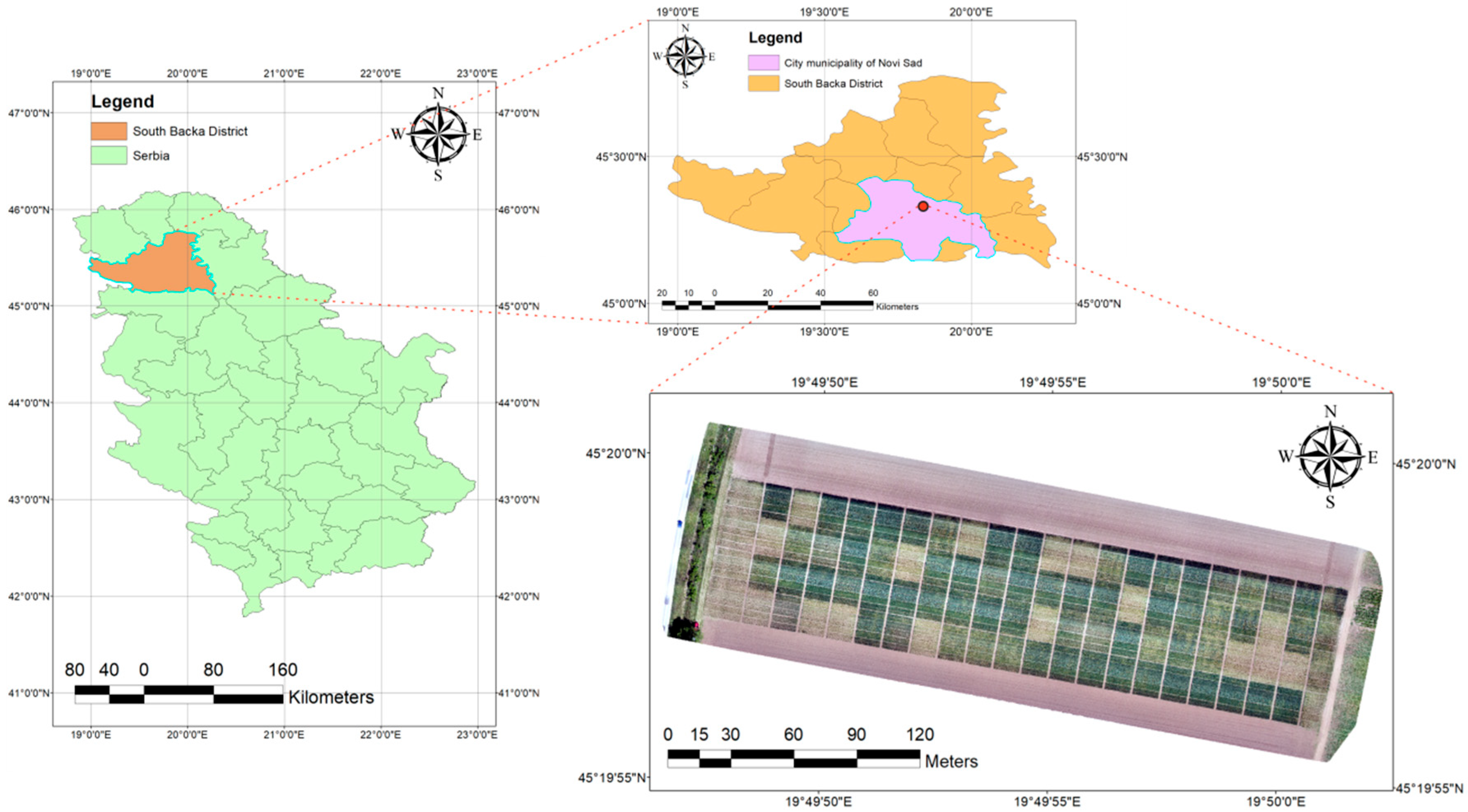
The study was part of a long-term experiment conducted by the Institute of Field and Vegetable Crops, Novi Sad, Vojvodina, Serbia. Its precise geographic coordinates are 45°19′58.0″ N, 19°49′53.6″ E, and it stands at an altitude of 82 m (Figure 1). The site was partitioned into 400 sub-plots, each spanning 5 × 10 m, methodically organized into a structured grid of 20 × 20. The soil at the site is the dominating soil type in the Vojvodina region, Haplic Chernozem Aric [15], and is characterized as highly fertile (approximately 43% of the total arable land).

Five distinct wheat cultivars were selected for the study: NS Igra, NS Rajna, NS Futura, NS Epoha, and NS Obala. The sowing density ranged between 200 and 230 kg/ha, contingent upon the specific cultivar. Critically, each cultivar was subjected to a diverse array of treatments, comprising twenty different NPK mineral fertilizer combinations. It is noteworthy that each of these treatments was replicated four times to ensure robustness in the findings.

The experiment aimed to create a diverse set of conditions, similar to the natural changes seen in farming fields. This matrix incorporated four hundred sub-plots, each interspersed with one of the five wheat cultivars, and was further nuanced by twenty distinct NPK treatment variations. This design allowed for variation changes in spectral channels, closely mimicking real-world farming events. This design not only accentuates the study’s precision but also enables the replication of naturally occurring agronomic phenomena in a controlled setting. For a detailed breakdown of NPK treatment combinations and the corresponding yields across each wheat cultivar, readers are directed to

Table 1. Comprehensive overview of NPK treatment combinations and corresponding yields for each wheat cultivar.

	Mineral Fertilization			Yield Intervals/Average Yield (t/ha)
Variant	N (kg/ha)	P (kg/ha)	K (kg/ha)	NS Igra	NS Rajna	NS Futura	NS Epoha	NS Obala
1	0	0	0	1.63–2.93 (2.3)	1.41–2.85 (2.26)	1.93–2.76 (2.29)	1.90–2.63 (2.33)	2.02–4.51 (2.97)
2	100	0	0	3.53–5.46 (4.73)	3.11–5.19 (4.53)	3.27–5.00 (4.32)	3.67–5.20 (4.59)	4.34–5.67 (5.15)
3	0	100	0	1.92–3.25 (2.53)	1.82–2.88 (2.46)	2.25–2.97 (2.60)	2.71–3.15 (2.96)	3.04–4.42 (3.63)
4	0	0	100	1.62–2.74 (2.21)	1.96–2.57 (2.16)	1.72–5.34 (2.97)	1.93–2.38 (2.22)	1.94–3.91 (2.66)
5	100	100	0	4.85–5.86 (5.38)	5.06–5.53 (5.34)	5.07–5.42 (5.25)	5.37–5.62 (5.48)	5.07–5.44 (5.29)
6	100	0	100	4.24–5.54 (4.82)	4.15–5.18 (4.72)	4.27–4.81 (4.49)	4.29–5.11 (4.73)	4.83–5.68 (5.16)
7	0	100	100	2.19–3.19 (2.72)	1.99–3.34 (2.69)	1.43–3.26 (2.47)	2.20–3.25 (2.81)	2.16–5.37 (3.70)
8	50	50	50	4.36–5.18 (4.83)	4.31–5.07 (4.64)	4.39–4.96 (4.67)	4.48–4.93 (4.66)	4.59–6.32 (5.23)
9	50	100	50	4.63–5.26 (5.03)	4.44–5.25 (4.91)	4.77–5.38 (5.06)	4.75–5.01 (4.88)	5.22–6.28 (5.54)
10	50	100	100	4.54–5.34 (4.91)	4.56–5.26 (4.94)	4.88–5.30 (5.13)	4.50–5.48 (4.97)	5.06–5.95 (5.42)
11	100	50	50	5.28–5.72 (5.46)	5.35–5.90 (5.62)	4.88–5.64 (5.35)	5.34–5.62 (5.48)	5.30–6.16 (5.62)
12	100	100	50	5.46–5.88 (5.65)	5.21–5.80 (5.53)	5.27–5.77 (5.61)	5.64–5.68 (5.66)	5.18–6.19 (5.64)
13	100	100	100	5.50–6.12 (5.73)	5.45–6.00 (5.82)	5.41–5.82 (5.66)	5.38–5.75 (5.52)	5.24–6.22 (5.67)
14	100	150	50	5.29–6.05 (5.70)	5.36–6.19 (5.79)	5.39–6.20 (5.78)	5.40–6.09 (5.73)	5.16–6.03 (5.50)
15	100	150	150	5.65–6.14 (5.89)	5.43–6.14 (5.86)	5.55–6.04 (5.81)	5.46–5.82 (5.68)	5.18–6.17 (5.62)
16	150	50	50	5.20–5.78 (5.38)	5.08–6.05 (5.63)	5.18–5.80 (5.47)	4.65–5.65 (5.12)	5.03–6.33 (5.46)
17	150	100	50	5.06–6.14 (5.64)	4.73–6.20 (5.48)	4.97–5.96 (5.49)	5.49–6.03 (5.74)	5.19–5.95 (5.52)
18	150	100	100	5.17–5.75 (5.50)	4.30–5.81 (5.34)	4.64–5.62 (5.36)	5.26–6.01 (5.67)	5.39–5.76 (5.51)
19	150	150	100	5.38–5.83 (5.64)	4.57–5.66 (5.19)	5.27–5.70 (5.50)	5.49–5.72 (5.65)	5.12–6.24 (5.65)
20	150	150	150	5.22–5.97 (5.46)	4.28–5.68 (4.92)	5.18–5.53 (5.28)	5.46–5.83 (5.69)	5.22–6.42 (5.65)

.

2.2. Unmanned Aerial Vehicle (UAV) Data Acquisition

For the purposes of data acquisition, high-resolution photographic images were captured on the following dates: 9 May 2022, during the Heading phase, 20 May 2022, during the Flowering phase, and 6 June 2022, during the Grainfilling phase. The DJI P4 Multispectral UAV, equipped with an MS camera, was utilized for this purpose. To ensure optimal lighting conditions and minimize potential sensor discrepancies, the aerial surveys were conducted under clear sky conditions, specifically between 12:00 and 13:00 h, corresponding to the local solar noon.

To ensure data consistency and flight stability, all UAV missions were conducted under wind speeds below 3 m/s, and identical flight parameters were maintained across all sessions, including altitude (30 m AGL), speed (3 m/s), and image overlap (75% both longitudinally and laterally). An autonomous waypoint-based flight plan was used in each session, allowing for precise replication of flight paths. Prior to every mission, the UAV system underwent a pre-flight checklist to ensure proper sensor calibration, battery condition, and GPS connectivity. Additionally, the same pilot operated all missions to reduce variability in execution.

The DJI P4 Multispectral, a quadrotor UAV (DJI, Shenzhen, China), was equipped with an integrated RGB camera and five distinct monochromatic sensors. These sensors encompass blue (B), green (G), red (R), red edge (RE), and near-infrared (NIR) bands, each tailored to specific spectral regions. Leveraging the data from the collected MS and RGB images, the study derived a set of 65 indices. This encompassed 40 MS and 25 RGB indices, offering a holistic perspective on the health and growth dynamics of the crop. A comprehensive specification of these monochromatic sensors can be found in

Table 2. Parameters of the monochromatic sensors of the multispectral camera.

Band	Center Wavelength/nm	Bandwidth/nm
Blue (B)	450	16
Green (G)	560	16
Red (R)	650	16
Red Edge (RE)	730	16
Near-infrared (NIR)	840	26

.

All flights were planned and executed using the DJI GS Pro software (Version: V2.0 2018.11, DJI, Shenzhen, China), ensuring consistent navigation and image capture parameters. The calibration of the sensors was verified prior to takeoff using the integrated sunlight sensor to normalize light intensity, ensuring reliable spectral readings across different times and dates.

When deployed at an operational altitude of 30 m, the UAV achieved a spatial resolution of 1.6 cm per pixel. To ascertain the drone’s geospatial accuracy during its flight, we employed the D-RTK 2 high-precision mobile station (DJI, Shenzhen, China). The camera’s exposure setting was calibrated to 2 s with specified flight margins set at 5 m. The imagery was systematically captured, with each mission covering an area of 2.7 hectares.

During our study, high-resolution imaging generated a substantial volume of data, culminating in a total digital footprint of 36.484 GB of raw data across three separate imaging sessions covering a combined area of 8.1 hectares. This yielded a digitization footprint of approximately 4.504 GB/ha per session. Each session entailed the acquisition of multispectral data across five spectral channels: blue, red, green, red-edge, and near-infrared, each contributing an equal partition of the overall data volume. Consequently, the digitization footprint for each spectral channel amounted to roughly 0.901 GB/ha per session.

Furthermore, orthomosaic images were created for each spectral channel in each of the three sessions, contributing an additional 7.898 GB in total to the digital footprint. When this is normalized across the total surveyed area, it results in an added digital footprint of approximately 0.975 GB/ha for the orthomosaic images.

Upon summing up the total data volume for all imaging sessions (36.484 GB) and the orthomosaic images (7.898 GB), a cumulative digital footprint of 44.382 GB was calculated. When this total digital footprint is normalized over the surveyed area of 8.1 hectares, an overall digitization footprint of approximately 5.479 GB per hectare was obtained.

In total, there were 9375 raw images captured across all sessions, with an even distribution across the five spectral channels, and the overall digitization footprint per session and per channel encompasses data from these individual images as well as from the compiled orthomosaic images.

The UAV’s flight plan was algorithmically generated using the DJI GS Pro software suite (DJI, Shenzhen, China). To ensure the UAV’s optimal navigational trajectory, a solar radiation spectral sensor was used. This facilitated adaptive adjustments of photographic parameters such as ISO, white balance, and shutter speed based on real-time solar irradiance data, eliminating the nuances of manual calibrations. The drone could maintain flight for 25 to 30 min on a single battery cycle.

2.3. Data Processing

Upon successful data retrieval using the DJI P4 Multispectral drone, Pix4D (Pix4Dmapper Enterprise 4.5.6, 2020, Pix4D, Prilly, Switzerland) software for a processing methodology was used, as delineated by [16]. This multifaceted workflow entailed the construction of an orthomosaic representation, aligning and amalgamating individual frames to architect a unified, geometrically congruent depiction of the experimental tract. Orthomosaic mappings for the entire RGB and MS bandwidths were subsequently synthesized, culminating in an ensemble of GeoTiff files. These georeferenced constructs not only summarized the raw image data but also provided rich metadata detailing the spatial orientation and geolocation of each constituent pixel.

The preprocessing steps included radiometric correction based on real-time sunlight intensity measurements from the onboard sunlight sensor, ensuring reflectance normalization across all spectral bands. Geometric correction was achieved using the D-RTK 2 high-precision GNSS base station, enabling accurate alignment of image coordinates. Furthermore, noise filtering and shadow reduction were automatically performed within the Pix4D pipeline, based on point cloud quality and texture variation.

In the subsequent phase, the synthesized GeoTiff datasets were integrated into the ArcGIS (ArcGIS-ArcMap 10.8.2, 2021, Esri Inc., 380 New York St, Redlands, CA, USA) platform for a granular analytical exercise, inspired by methodologies presented by [17]. A salient feature of this exploration was the derivation of numerical metrics for the RGB and MS spectra across each delineated plot. Additionally, the extraction of statistical descriptors for each demarcated polygonal segment within the experimental expanse was conducted.

2.4. Development of RGB and MS Indices Leveraging Extracted Spectral Data

This study dissected and analyzed the numerical representations associated with the intensities observed within the red, blue, and green spectral sections, supplemented by data from the red-edge domain and the near-infrared region. After extracting these spectral data, equations for RGB and MS indices were derived, as specifically outlined in

Table A1. Vegetation indices, accompanied by their computational equations, derived from the numerical intensities of RGB bands [3].

Index Type	Formula
Red (R), Green (G), Blue (B)	Numerical values
Normalized Red	$r={\displaystyle \frac{Red}{Red+Green+Blue}}$
Normalized Green	$g={\displaystyle \frac{Green}{Red+Green+Blue}}$
Normalized Blue	$b={\displaystyle \frac{Blue}{Red+Green+Blue}}$
Green–Red Ratio Index	$GRRI={\displaystyle \frac{Green}{Red}}$
Green–Blue Ratio Index	$GBRI={\displaystyle \frac{Green}{Blue}}$
Red–Blue Ratio Index	$RBRI={\displaystyle \frac{Red}{Blue}}$
Excess Red Vegetation Index	$ExR=1.4·r-g$
Excess Green Vegetation Index	$ExG=2·g-r-b$
Excess Blue Vegetation Index	$ExB=1.4·b-g$
Excess Green Minus Excess Red Index	$ExGR=ExG-ExR$
Woebbecke Index	$WI={\displaystyle \frac{Green-Blue}{Green+Red}}$
Normalized Difference Index	$NDI={\displaystyle \frac{r-g}{r+g+0.01}}$
Color Intensity	$INT={\displaystyle \frac{Red+Blue+Green}{3}}$
Green Leaf Index 1	$GLI1={\displaystyle \frac{2·Green-Red-Blue}{2·Green+Red+Blue}}$
Green Leaf Index 2	$GLI2={\displaystyle \frac{2·Green-Red+Blue}{2·Green+Red+Blue}}$
Vegetative Index	$VEG={\displaystyle \frac{{Red}^{\left(2/3\right)}·b^{\left(1/3\right)}}{Red}}$
Color Index of Vegetation	$CIVE=0.441·r-0.811·g+0.3856·b+18.79$
Combination	$COM=0.25·ExG+0.3·ExGR+0.33·CIVE+0.12·VEG$
Normalized Green–Red Vegetation Index	$NGRVI={\displaystyle \frac{Green-Red}{Green+Red}}$
Kawashima Index	$IKAW={\displaystyle \frac{Red-Blue}{Red+Blue}}$
Visible-band difference vegetation Index	$VDVI={\displaystyle \frac{2·g-r-b}{2·g+r+b}}$
Visible Atmospherically Resistance Index	$VARI={\displaystyle \frac{g-r}{g+r-b}}$
Principal Component Analysis Index	$IPCA=0.994·\left|Red-Blue\right|+0.961·\left|Green-Blue\right|+0.914·\left|Green-Red\right|$
Modified Green–Red Vegetation Index	$MGRVI={\displaystyle \frac{{Green}^2-{Red}^2}{{Green}^2+{Red}^2}}$
Red–Green–Blue Vegetation Index	$RGBVI={\displaystyle \frac{{Green}^2-Blue·Red}{{Green}^2+Blue·Red}}$

and

Table A2. Vegetation indices, along with their associated equations, found on the numerical intensities of MS bands.

Index Type	Formula	Reference
Normalized Difference Vegetation Index	$NDVI={\displaystyle \frac{NIR-Red}{NIR+Red}}$	[6]
Renormalized Difference Vegetation Index	$RDVI={\displaystyle \frac{NIR-Red}{{\left(NIR+Red\right)}^{1/2}}}$	[7]
Difference vegetation index	$DVI=NIR-Red$	[4]
Blue normalized difference vegetation index	$BNDVI={\displaystyle \frac{NIR-Blue}{NIR+Blue}}$	[6]
Green normalized difference vegetation index	$GNDVI={\displaystyle \frac{NIR-Green}{NIR+Green}}$	[37]
Modified Soil Adjusted Vegetation Index	$MSAVI={\displaystyle \frac{2NIR+1-\sqrt{{\left(2NIR+1\right)}^2-8\left(NIR-Red\right)}}{2}}$	[38]
Red-Edge Chlorophyll Vegetation Index	$ReCI={\displaystyle \frac{NIR}{Red-1}}$	[39]
Normalized Difference Red Edge Index	$NDRE={\displaystyle \frac{NIR-RedEdge}{NIR+RedEdge}}$	[37]
Normalized Difference Water Index	$NDWI={\displaystyle \frac{Green-NIR}{Green+NIR}}$	[40]
Optimized Soil-Adjusted Vegetation Index	$OSAVI=\left(1+0.16\right)·{\displaystyle \frac{\left(NIR-Red\right)}{\left(NIR+Red+0.16\right)}}$	[37]
The Simple Ratio	$SR={\displaystyle \frac{NIR}{Red}}$	[37]
Modified Simple Radio	$MSR={\displaystyle \frac{\frac{NIR}{Red}-1}{{\left(\frac{NIR}{Red}\right)}^{1/2}+1}}$	[41]
Infrared percentage vegetation index	$IPVI={\displaystyle \frac{NIR}{NIR+Red}}$	[38]
Enhanced Vegetation Index	$EVI={\displaystyle \frac{2.5·\left(NIR-Red\right)}{\left(NIR+6·Red-7.5·Blue+1\right)}}$	[42]
Green atmospherically resistant vegetation index	$GARI={\displaystyle \frac{\left(NIR-\left(Green-\left(Blue-Red\right)\right)\right)}{\left(NIR-\left(Green+\left(Blue-Red\right)\right)\right)}}$	[43]
Soil-Adjusted Vegetation Index	$SAVI={\displaystyle \frac{\left(NIR-Red\right)}{\left(NIR+Red+0.5\right)}}·(1+0.5)$	[38]
Green Soil Adjusted Vegetation Index	$GSAVI={\displaystyle \frac{\left(NIR-Green\right)}{\left(NIR+Green+0.5\right)}}·(1+0.5)$	[44]
Green Optimized Soil Adjusted Vegetation Index	$GOSAVI={\displaystyle \frac{NIR-Green}{NIR+Green+0.16}}$	[44]
Green Chlorophyll Vegetation Index	$GCI={\displaystyle \frac{NIR}{Green}}-1$	[45]
Plant Senescence Reflectance Index	$PSRI={\displaystyle \frac{Red-Green}{NIR}}$	[46]
Nonlinear vegetation index	$NLI={\displaystyle \frac{{NIR}^2-Red}{{NIR}^2+Red}}$	[47]
Transformed difference vegetation index	$TDVI=1.5·{\displaystyle \frac{\left(NIR-Red\right)}{\sqrt{\left({NIR}^2+Red+0.5\right)}}}$	[48]
Visible Atmospherically Resistant Index	$VARI={\displaystyle \frac{Green-Red}{Green+Red-Blue}}$	[49]
Wide Dynamic Range Vegetation Index	$WDRVI={\displaystyle \frac{0.1NIR-Red}{0.1NIR+Red}}$	[43]
Green-Red NDVI	$GRNDVI={\displaystyle \frac{NIR-\left(Green+Red\right)}{NIR+\left(Green+Red\right)}}$	[41]
Green-Blue NDVI	$GBNDVI={\displaystyle \frac{NIR-\left(Green+Blue\right)}{NIR+\left(Green+Blue\right)}}$	[50]
Red-Blue NDVI	$GRNDVI={\displaystyle \frac{NIR-\left(Red+Blue\right)}{NIR+\left(Red+Blue\right)}}$	[50]
Pan NDVI	$PNDVI={\displaystyle \frac{NIR-\left(Green+Red+Blue\right)}{NIR+\left(Green+Red+Blue\right)}}$	[50]
Simple Ratio Red/NIR Ratio Vegetation-Index	$ISR={\displaystyle \frac{Red}{NIR}}$	[51]
Leaf Chlorophyll Index	$LCI={\displaystyle \frac{NIR-RedEdge}{NIR+Red}}$	[4]
Ratio Between NIR and Green Bands	${VI}_{\left({\displaystyle \frac{NIR}{Green}}\right)}={\displaystyle \frac{NIR}{Green}}$	[52]
Ratio Between NIR and Red Edge Bands	${VI}_{\left({\displaystyle \frac{NIR}{RedEdge}}\right)}={\displaystyle \frac{NIR}{RedEdge}}$	[53]
Simplified Canopy Chlorophyll Content Index	$SCCCI={\displaystyle \frac{NDRE}{NDVI}}$	[3]
Modified Chlorophyll Absorption Reflectance Index	$MCARI=\left(RedEdge-Red-0.2·\left(RedEdge-Green\right)\right)·{\displaystyle \frac{RedEdge}{Red}}$	[4]
Transformed Chlorophyll Absorption Reflectance Index	$TCARI=3·\left((RedEdge-Red)-0.2·\left(RedEdge-Green\right)·{\displaystyle \frac{RedEdge}{Red}}\right)$	[37]
Structure Insensitive Pigment Index	$SIPI={\displaystyle \frac{NIR-Blue}{NIR-Red}}$	[41]
TCARI/OSAVI	${\displaystyle \frac{TCARI}{OSAVI}}$	[41]
MCARI/OSAVI	${\displaystyle \frac{MCARI}{OSAVI}}$	[41]
Red-Edge Chlorophyll Index 1	$CI1={\displaystyle \frac{NIR}{RedEdge}}-1$	[54]
Red-Edge Chlorophyll Index 2	$CI2={\displaystyle \frac{RedEdge}{Green}}-1$	[55]

, in the Appendix A, based on the methodologies presented in the scientific paper by [3]. The application of such indices provides a profound comprehension of the spectral characteristics of the analyzed terrain, elucidating details about their intrinsic physical and optical properties. At the specific stages of development and with the planting density employed, the canopy of the wheat plants is closed such that soil visibility through the canopy is almost nonexistent. Therefore, background noise such as soil and shadows was minimal and did not significantly impact the analysis. This dense canopy ensures that the measurements are primarily from the wheat plants themselves, providing accurate canopy information.

2.5. Applying the PyCaret Library for Yield Prediction

PyCaret is an open-source, high-level machine-learning library that offers efficient data preparation and modeling through a simple and user-friendly API [18]. The key step of this research is applying the PyCaret software on MS and RGB indices obtained by using UAVs for yield estimation. For that purpose, the correlation coefficient between the collected vegetation indices and the actual yield was examined. This step was necessary to statistically establish the relationship between the 65 calculated vegetation indices and the actual yield. After that, the normalization of 65 numerical features of the dataset was performed using the z-score method. This step is crucial for machine-learning algorithms sensitive to feature scales, as it transforms each feature to have a mean of zero and a standard deviation of one. Normalization of the features resulted in a quicker convergence of the algorithm, ultimately leading to more generalizable and robust predictions. These normalized indices were then matched with corresponding yield data collected manually from the field. This approach led to the establishment of a database containing 400 observations, each encompassing 66 feature variables, including 65 vegetation indices and wheat yield, which was employed in this research. Upon initialization, a unique session identifier (Session ID: 4797) was generated to facilitate the reproducibility of the experiment, in accordance with good scientific practice. Before training, the entire set of 65 vegetation indices was retained without applying automatic feature selection or dimensionality reduction techniques. This decision was made to preserve the full spectral information available in the dataset, allowing the machine-learning algorithms to independently evaluate the relevance of each index during model fitting. Since the PyCaret library internally handles algorithm-specific regularization and weight assignment, models such as Lasso, Ridge, and tree-based ensembles inherently perform implicit feature prioritization during training. The data was divided into a training set and a test set, with 280 and 120 samples (0.7/0.3 ratio), respectively. This partitioning was implemented to allow for robust training and evaluation of machine-learning models. The variable targeted for regression was denoted as ‘Yield’, which represents the wheat yield that the experiment aims to predict. Using machine-learning algorithms, the software learns how to recognize patterns and relationships between MS and RGB indices and yield data. Through an iterative process, the software is optimized to achieve as accurate a yield estimation as possible.

A 10-fold cross-validation approach was implemented to evaluate the models’ performance, using the KFold algorithm exclusively on the training set. In this process, each fold was used once as a validation set while the k-1 remaining folds were used for the training. This validation technique provides a robust way to assess the model’s performance within the training set, minimizing the bias and variance associated with a single random partition of this subset. The built-in ‘tune model’ function of PyCaret used in our study enables automated hyperparameter tuning on the training folds, reducing manual effort and expertise required to optimize model performance within the training data. This process ensures that the model is not only optimized but also validated in a rigorous manner before being finally evaluated on a separate test set, which is critical in scientific studies where optimum model settings are essential and need to be validated effectively [19].

The tuning process utilizes grid search and random search strategies internally, depending on the algorithm, and selects hyperparameters based on performance metrics such as R² and RMSE across the cross-validation folds. All optimization steps were automated and reproducible, contributing to model stability.

After completing the learning process, PyCaret software (Version: 3.0, Toronto, ON, Canada) can apply the learned models to new MS and RGB indices data to estimate crop yields on agricultural crop fields.

In this study, 25 regression algorithms available in PyCaret were employed to evaluate their performance on the task of wheat yield prediction. These include traditional linear models such as Linear Regression (lr), Lasso (lasso), and Ridge (ridge), as well as ensemble methods like Random Forest Regressor (rf), Gradient Boosting Regressor (gbr), Extra Trees Regressor (et), AdaBoost Regressor (ada), and advanced machine-learning models such as Support Vector Regression (svm), Multi-Layer Perceptron Regressor (mlp), and Extreme Gradient Boosting (xgboost). A complete list of the models and their abbreviations is provided in

Table A3. List of Regression Models with Corresponding Abbreviations.

Model Type	Model Abbreviation
Linear Regression	lr
Lasso Regression	lasso
Ridge Regression	ridge
Elastic Net	en
Least Angle Regression	lar
Lasso Least Angle Regression	llar
Orthogonal Matching Pursuit	omp
Bayesian Ridge	br
Automatic Relevance Determination	ard
Passive Aggressive Regressor	par
Random Sample Consensus	ransac
TheilSen Regressor	tr
Huber Regressor	huber
Kernel Ridge	kr
Support Vector Regression (SVR)	svm
K Neighbors Regressor	knn
Decision Tree Regressor	dt
Random Forest Regressor	rf
Extra Trees Regressor	et
AdaBoost Regressor	ada
Gradient Boosting Regressor	gbr
MLP Regressor	mlp
Extreme Gradient Boosting	xgboost
Light Gradient Boosting Machine	lightgbm
Dummy Regressor	dummy

in the Appendix A. This comprehensive comparison enabled the identification of models that best capture nonlinear and complex relationships between vegetation indices and yield.

2.6. Model Performance Metrics in Yield Prediction

Evaluating the performance of machine-learning models in the context of yield prediction is a crucial step to understanding the model’s efficacy and reliability. Several metrics are commonly employed to quantify various aspects of the model’s predictive ability. Below, we elucidate some of the following key performance indicators used in this study [3]:

• Mean Absolute Error (MAE)

The Mean Absolute Error (1) measures the average of the absolute differences between the predicted and observed values. It quantifies the accuracy of the model in predicting the yield by giving a straightforward interpretation of how far off the predictions are on average.

$$\mathrm{M}\mathrm{A}\mathrm{E}={\displaystyle \frac{1}{n}}{\sum }_{i=1}^n\left|y_i-{\widehat{y}}_i\right|$$

(1)

In the evaluation metrics, n denotes the total number of samples in the dataset, and i serves as the index for each sample during summation. The symbol y represents the observed (or actual) value of the target variable for the i-th sample, while ${\widehat{y}}_i$ stands for the model-predicted value for the same i-th sample.

• Mean Squared Error (MSE)

The Mean Squared Error (2) is an indicator of the quality of an estimator. It measures the average of the squares of the differences between observed and predicted values. The MSE is more sensitive to outliers compared to the MAE.

$$\mathrm{M}\mathrm{S}\mathrm{E}={\displaystyle \frac{1}{n}}{\sum }_{i=1}^n{\left(y_i-{\widehat{y}}_i\right)}^2$$

(2)

• Root Mean Squared Error (RMSE)

The Root Mean Squared Error (3) is the square root of the MSE. It provides a measure of the magnitude of error between the predicted and observed values, with higher emphasis on larger errors.

$$\mathrm{R}\mathrm{M}\mathrm{S}\mathrm{E}=\sqrt{{\displaystyle \frac{1}{n}}{\sum }_{i=1}^n{\left(y_i-{\widehat{y}}_i\right)}^2}$$

(3)

• Coefficient of Determination (R²)

The R-squared (4) metric provides a measure of how well the predicted outcomes explain the variance in the actual output values. It ranges from 0 to 1, with higher values indicating a better fit of the model to the observed data.

$${\mathrm{R}}^2=1-{\displaystyle \frac{SSR}{SST}}$$

(4)

where: The Sum of Squares of Residuals (SSR) (5) is a crucial metric that quantifies the sum of the squared differences between the actual (observed) and predicted values. Mathematically, it is defined as follows:

$$SSR={\sum }_{i=1}^n{\left(y_i-{\widehat{y}}_i\right)}^2$$

(5)

and the Total Sum of Squares (SST) (6), also known as the total sum of squares about the mean, quantifies the sum of squared differences between the actual (observed) values and the mean value of the target variable. It is mathematically expressed as follows:

$$SST={\sum }_{i=1}^n{\left(y_i-{\overline{y}}_i\right)}^2$$

(6)

The ${\overline{y}}_i$ symbol signifies the mean value of the target variable across all samples.

• Root Mean Square Logarithmic Error (RMSLE)

The RMSLE (7) is particularly useful when the errors have a wide range, and you wish to penalize underestimates more than overestimates. It is the square root of the average of the squared logarithmic differences between the predicted and observed values.

$$\mathrm{R}\mathrm{M}\mathrm{S}\mathrm{L}\mathrm{E}=\sqrt{{\displaystyle \frac{1}{n}}{\sum }_{i=1}^n{\left(\mathrm{l}\mathrm{o}\mathrm{g}\left(y_i+1\right)-\mathrm{l}\mathrm{o}\mathrm{g}\left({\widehat{y}}_i+1\right)\right)}^2}$$

(7)

• Mean Absolute Percentage Error (MAPE)

MAPE (8) is a measure of prediction accuracy expressed as a percentage. It is calculated as the average of the absolute percentage differences between the observed and predicted values.

$$\mathrm{M}\mathrm{A}\mathrm{P}\mathrm{E}={\displaystyle \frac{100}{n}}{\sum }_{i=1}^n\left|{\displaystyle \frac{y_i-{\widehat{y}}_i}{y_i}}\right|$$

(8)

• Time Taken (TT)

The Time Taken (TT) in seconds is an important metric in practical applications. It gives an idea of the computational efficiency of the algorithm, which is crucial when dealing with large-scale datasets or real-time predictions.

TT (Sec) = Total Time taken for model training and evaluation in seconds.

3. Results

3.1. Overview of Wheat Yield Variability Among Different Cultivars

In

Table 3. Descriptive analysis of wheat yields across selected cultivars.

Descriptive Statistics	Cultivars
	NS Igra	NS Rajna	NS Futura	NS Epoha	NS Obala
Avg yield (t/ha)	4.78	4.69	4.73	4.78	5.03
Max yield (t/ha)	6.14	6.20	6.20	6.09	6.42
Min yield (t/ha)	1.62	1.41	1.43	1.90	1.94
STDEV	1.28	1.29	1.24	1.20	1.09
CV (%)	26.74	27.55	26.18	25.19	21.63

, a comprehensive range of yields obtained from five different wheat varieties is showcased, serving as the foundational data for the development of our mathematical model. This wide spectrum of yield values is an integral part of the experimental setup and contributes to the versatile applicability of the resulting prediction models, which was the key objective of the experiment. Despite variations in yields among different wheat varieties, the results have facilitated the development of a reliable and flexible mathematical model for yield estimation.

To further clarify the observed variability, it is important to briefly outline the specific characteristics of the included cultivars. NS Obala achieved the highest average yield (5.03 t/ha) with the lowest coefficient of variation (21.63%), consistent with its description as a highly productive and robust cultivar with tall plants and excellent adaptability. NS Rajna recorded the lowest average yield (4.69 t/ha) and the highest variability (CV = 27.55%), which aligns with its medium-late maturity and slightly lower stress tolerance. NS Igra and NS Epoha, both with similar average yields (4.78 t/ha), are characterized by strong disease resistance and adaptability across soil types. NS Futura exhibited stable performance and favorable yield potential, supported by excellent cold tolerance, higher thousand-kernel weight, and responsiveness to nitrogen fertilization. These differences reflect the genetic and agronomic diversity of the cultivars and strengthen the foundation for robust model development.

3.2. Correlation Coefficients Between Indices and Wheat Yield

The examination of correlation coefficients between vegetation indices and wheat yield was conducted for all three distinct measurement dates based on MS and RGB indices.

For the MS indices collected on 9 May 2022, the absolute average correlation coefficient across the three dates stood at 0.92, with a standard deviation of 0.04. All correlation coefficients for this date are provided in Figure A2 in the Appendix A section. On 20 May 2022, the corresponding figures were 0.92 and 0.05, with all correlation coefficients for this date provided in Figure A3 in the Appendix A section. For the last measurement conducted on 6 June 2022, they were 0.82 and 0.17, with all correlation coefficients for this date available in Figure A4 in the Appendix A section.

Concerning the RGB index measurements on 9 May 2022, the absolute average correlation coefficient across the three dates was 0.83, with a standard deviation of 0.2. On 20 May 2022, these values were 0.78 and 0.18, while on 6 June 2022, they were 0.40 and 0.19.

A more in-depth analysis reveals a strong correlation between specific indices and wheat yield. It is noteworthy that the majority of MS indices displayed a robust correlation with wheat yield, with approximately 90% (36 out of 40) of MS indices for the measurement conducted on 9 May 2022, 85% (34 out of 40) for 20 May 2022, and 82.5% (33 out of 40) for 6 June 2022, exhibiting a correlation coefficient exceeding 0.8 or falling below −0.8, signifying a high correlation. In contrast, RGB indices exhibited a more diverse range of correlation strengths. For instance, on 9 May 2022, around 60% (15 out of 25) of RGB indices displayed such high correlation, while on 20 May 2022, this was the case for approximately 52% (13 out of 25), and on 6 June 2022, only 44% (11 out of 25). This observation implies that, in general, MS indices demonstrated a more consistent and stronger correlation with wheat yield in comparison to RGB indices.

The enhanced performance of MS indices can be explained by their incorporation of additional spectral bands, particularly the near-infrared (NIR) and red-edge (RE) wavelengths. These bands are highly sensitive to key physiological traits such as chlorophyll concentration, canopy structure, and water content—parameters directly associated with crop productivity. As wheat progresses through phenological stages like Heading, Flowering, and Grainfilling, variations in leaf area index, pigment composition, and biomass become more pronounced, and MS indices such as NDVI, SIPI, and RENDVI are particularly adept at capturing these dynamics. On the other hand, RGB indices—relying solely on visible spectrum data—lack the spectral depth to reflect internal physiological processes with comparable precision. Their greater sensitivity to ambient lighting and surface reflectance conditions also contributes to their lower and more variable correlation with yield. This spectral and physiological sensitivity inherent to MS indices underpins their stronger and more stable association with yield observed across all measurement dates.

These results underscore the justification for utilizing both MS and RGB indices for wheat yield prediction purposes. The statistical significance of the calculated correlation coefficients between the yield variable and the observed indices was assessed using a t-test. It was found that the relationship between the yield variable and the observed indices was highly statistically significant in all cases for measurements conducted on 9 May 2022. For measurements taken on 20 May 2022, all correlation coefficients were statistically significant at the alpha = 0.01 significance level, except for the correlation coefficient between yield and the WI index, which was significant at the alpha = 0.05 level. For measurements conducted on 6 June 2022, all correlation coefficients were statistically significant at the alpha = 0.01 significance level, except for the correlations between yield and the indices PSRI, VEG, IKAW, and IPCA, where no statistically significant correlation was recorded. The exclusion of indices with correlation levels less than 0.8 or greater than −0.8 may lead to a reduction in the accuracy and comprehensiveness of the selected models. Given that certain vegetation indices, while having a low correlation in one instance, may exhibit a high correlation in another, they indeed have a significant role in model creation. It is worth emphasizing that the PyCaret machine-learning system autonomously assigns importance to each vegetation index in the creation of specific prediction models, depending on their correlation with yield. This approach ensures high-precision outcomes while maintaining model comprehensiveness.

3.3. Analysis of Regression Model Performance

The subsequent evaluation provides an in-depth analysis of various regression models employed for predicting wheat yield. The results of the first five highly ranked yield prediction models, based on the test set data, are presented in

Table 4. Performance metrics of regression models for 9 May 2022.

Model	MAE	MSE	RMSE	R2	RMSLE	MAPE	TT (Sec)
Support Vector Regression	0.2065	0.0701	0.2592	0.9465	0.0454	0.0454	0.037
Ridge Regression	0.2114	0.0697	0.2601	0.9462	0.0450	0.0460	0.045
Huber Regressor	0.2117	0.0715	0.2617	0.9455	0.0463	0.047	0.114
Bayesian Ridge	0.2134	0.0712	0.2632	0.9451	0.0452	0.0462	0.070
Automatic Relevance Determination	0.2130	0.0711	0.2629	0.9449	0.0453	0.0461	0.209

,

Table 5. Performance metrics of regression models for 20 May 22022.

Model	MAE	MSE	RMSE	R2	RMSLE	MAPE	TT (Sec)
MLP Regressor	0.2173	0.0791	0.2778	0.9351	0.0500	0.0492	0.455
Extra Trees Regressor	0.2181	0.0783	0.2760	0.9326	0.0504	0.0496	0.512
Random Forest Regressor	0.2186	0.0784	0.2764	0.9326	0.0502	0.0494	0.792
Light Gradient Boosting Machine	0.2227	0.0827	0.2844	0.9311	0.0523	0.0506	1.481
Support Vector Regression	0.2286	0.0841	0.2882	0.9288	0.0524	0.0517	0.035

and

Table 6. Performance metrics of regression models for 6 June 2022.

Model	MAE	MSE	RMSE	R2	RMSLE	MAPE	TT (Sec)
Support Vector Regression	0.2573	0.1118	0.3288	0.9086	0.0652	0.0617	0.024
Light Gradient Boosting Machine	0.2710	0.1175	0.3384	0.9057	0.0650	0.0626	0.244
Random Forest Regressor	0.2641	0.1179	0.3404	0.9046	0.0664	0.0615	0.594
Extra Trees Regressor	0.2701	0.1183	0.3409	0.904	0.0663	0.0629	0.224
Ridge Regression	0.2821	0.1252	0.3499	0.8986	0.0705	0.0676	0.034

. Although only the top five performing models are presented for each measurement date to enhance clarity and avoid excessive tabular content, all 25 machine-learning regression models listed in Table A3 were consistently applied to each dataset, and their performance was evaluated accordingly.

The performance metrics displayed in Table 4, Table 5 and Table 6 offer valuable insights into the effectiveness of various regression models for predicting wheat yield across different measurement dates. The hyperparameters for the top models for each date, selected based on performance metrics, are detailed in

Table A4. Hyperparameters of the Support Vector Regression Model for 9 May 2022. and 6 June 2022.

Hyperparameter	Value	Hyperparameter	Value
kernel	rbf	degree	3
coef0	0	Tol	0.001
C	1	epsilon	0.1
shrinking	True	cache_size	200
max_iter	−1	gamma	scale

and

Table A5. Hyperparameters of the MLP Regressor Model for 20 May 2022.

Hyperparameter	Value	Hyperparameter	Value
hidden_layer_sizes	(100)	activation	relu
solver	adam	Alpha	0.0001
batch_size	auto	learning_rate	constant
learning_rate_init	0.001	power_t	0.5
max_iter	500	Shuffle	True
momentum	0.9	Tol	0.0001
beta_1	0.9	nesterovs_momentum	True
epsilon	1.00 × 10−8	validation_fraction	0.1
beta_2	0.999	n_iter_no_change	10

in the Appendix A.

Table 4 showcases the model performance for 9 May 2022. Notably, all five models show impressive results. These models consistently achieve similar metrics performance, and all of them indicate accurate predictions.

Moving to Table 5, which represents the performance on 20 May 2022, we observe similar accuracy of regression models. However, in this case, according to statistical indicators of model accuracy, the MLP Regressor is ranked highest, while the SVR is only in fifth place. There is a very small difference in the accuracy of these models. According to statistical indicators, the difference in the accuracy of wheat yield prediction is almost negligible.

In Table 6, corresponding to 6 June 2022, the models, particularly SVR, maintain a good level of accuracy.

When comparing performance across the three dates, it is evident that the prediction accuracy tends to slightly decrease over time. For instance, the best-performing model on 9 May (SVR) achieved an R² of 0.9465 and RMSE of 0.2592, while on 20 May, the best-performing model (MLP Regressor) recorded an R² of 0.9351 and RMSE of 0.2778. By 6 June, the top model (SVR) exhibited further reduced performance with an R² of 0.9086 and RMSE of 0.3288. This trend reflects a gradual decline in prediction accuracy as the wheat approaches later growth stages, possibly due to saturation in spectral data or increased variability in field conditions. Despite this, all models maintained a relatively high level of accuracy throughout the period.

The ranking of models also varies slightly with date, which may be attributed to differences in the nature and informativeness of the data collected at each phenological stage. For example, while SVR and Ridge Regression performed best early in the season (9 May), ensemble-based models like Random Forest Regressor and Extra Trees Regressor showed competitive performance on 20 May and 6 June. These fluctuations underscore the importance of measurement timing in yield prediction and suggest that mid-season data may offer more consistent prediction quality across model types.

These results collectively underscore the robust performance of the regression models in predicting wheat yield across multiple dates. The consistently good performance of metrics indicates their reliability in wheat yield estimation, making them valuable tools for agricultural decision-making and precision agriculture applications.

3.4. Detailed Performance Analysis of Top Regression Models for Each Date

In a more detailed assessment conducted on the entire dataset for each date, the best regression models for those dates exhibited distinct performance characteristics. In the forthcoming analysis, the diagrams presented in the subsequent Figure 2 provide a visual representation of these models’ performances on specific evaluation dates, elucidating their predictive capabilities in detail.

• 9 May 2022—SVR Model Analysis:

• Performance Metrics: The model achieved a training R² of 0.957 and a test R² of 0.947. In the context of predicting wheat yield, such high R² values signify an exceptional degree of accuracy.
• Residual Plot Analysis: The plot for this date shows that the residuals are tightly packed around the zero line, indicating a robust model performance. The minor spread of residuals in some regions indicates a few prediction inaccuracies, but overall, the model seems to have captured the major underlying patterns in the data.
• Distribution Analysis: The histogram on the right showcases a nearly normal distribution of residuals with a slight right skew, hinting towards minor prediction biases.

• 20 May 2022—MLP Regressor Model Analysis:

• Performance Metrics: The model achieved a training R² of 0.968 and a test R² of 0.938. An R² value nearing 0.97 for training data and 0.94 for test data highlights the model’s ability to capture the relationships within the data effectively.
• Residual Plot Analysis: The residuals, for the most part, cluster around the zero line, signifying accurate predictions. However, there is a noticeable spread in certain areas, especially around the middle predicted values, suggesting potential outliers or complex patterns that the model may not have entirely grasped.
• Distribution Analysis: The histogram portrays a slightly bimodal distribution, indicating two dominant types of prediction errors or two dominant groups in the data.

• 6 June 2022 SVR Model Analysis:

• Performance Metrics: For this date, the model produced a training R² of 0.937 and a test R² of 0.916. Although these numbers are somewhat lower than those from the previous dates, they still indicate strong predictive performance. With an explanation of over 93% of the data variance, the model remains valuable for agricultural planning and optimization based on its forecasts.
• Residual Plot Analysis: The residuals, although mostly surrounding the zero line, showcase a more dispersed pattern as compared to the SVR model evaluated on 9 May 2022. This indicates a slightly lesser prediction accuracy for this specific dataset.
• Distribution Analysis: The distribution of residuals on the right displays a near-normal pattern, albeit with a hint of right skewness, pointing towards minor prediction biases.

While individual model diagnostics for each date provide granular insight, comparing residual plots and distribution shapes reveals broader trends. For example, the increase in residual spread from 9 May to 6 June reflects growing prediction uncertainty as the wheat matures. This could be linked to increasing canopy closure and spectral saturation in later stages, reducing the distinctiveness of vegetation indices. Additionally, the shift from nearly normal residual distributions to slightly skewed or bimodal forms suggests more complex error structures in later measurements, possibly due to field heterogeneity or weather variability. These insights imply that while regression models perform well throughout the season, their precision may be highest during the heading to flowering phases, as captured in the earlier dates.

Considering the regression models’ performance on three distinct evaluation dates, the diagrams illustrating their capabilities are presented in Figure 3.

• 9 May 2022—SVR Model Analysis:

• Performance Metrics: The SVR model on this date achieved an R² value of 0.947. In the context of wheat yield predictions, this high R² shows the model’s accuracy. It indicates that the model can effectively capture most of the data variance, making it reliable for wheat yield predictions.
• Diagram Insight: The plot portrays predicted values against true values. A closer alignment of points with the identity line indicates better predictions. While most data points align with the “best fit” line, slight deviations highlight the model’s areas of potential improvement.

• 20 May 2022—MLP Regressor Model Analysis:

• Performance Metrics: The MLP Regressor on this date recorded an R² of 0.938. Even though marginally lower than the SVR model on 9 May 2022, it remains high in accuracy.
• Diagram Insight: The plotted data points largely follow the identity line, suggesting a good match between predicted and actual values. However, a few data points diverge, suggesting areas where the model might have faced challenges, possibly due to intricate patterns or outliers in the dataset.

• 6 June 2022—SVR Model Analysis:

• Performance Metrics: On this date, the SVR model reported an R² of 0.916. While slightly lower than previous results, an R² above 0.9 in agriculture still highlights a strong predictive capability.
• Diagram Insight: Most data points are near the identity line, showing the model’s consistency in predictions. The scatter, although slightly more pronounced compared to the evaluation of 9 May 2022, is still within acceptable bounds for wheat yield forecasting.

In summary, both the residual analysis and predicted-vs-actual plots confirm the stability of model performance across all dates, while also revealing subtle variations that are relevant for practical implementation. The slightly declining accuracy and increasing residual dispersion over time underscore the importance of early-season data collection for maximizing prediction precision. These findings support the integration of temporal optimization in UAV-based monitoring workflows.

Furthermore, the observed fluctuations in model rankings across dates can also be attributed to the intrinsic sensitivity of individual algorithms to the underlying data distribution and noise patterns. For instance, Support Vector Regression (SVR), which relies on optimal margin boundaries, may perform exceptionally well when the data exhibits linear or quasi-linear trends with minimal noise, as observed on 9 May and 6 June. However, on 20 May, where data characteristics may have been more nonlinear or affected by subtle outliers, the MLP Regressor, known for its capability to capture complex patterns through neural layers, outperformed SVR. These differences highlight the importance of aligning model selection with data-specific traits, ensuring the robustness of predictive analytics in agricultural scenarios.

The results from the specified evaluation dates provide a nuanced understanding of the different regression models’ capabilities. While each model showed high predictive power, subtle differences in performance metrics and visual insights underline the importance of continuous evaluation. It is evident that, while all models offer high value in predicting wheat yield, their effectiveness can vary depending on the data’s characteristics and complexities. This rigorous assessment underscores the significance of selecting the right model for specific datasets and the need for ongoing validation to ensure optimal performance in the field of wheat yield prediction.

4. Discussion

The findings from this study can offer novel insights into the application of machine learning for predicting wheat yields [19]. The following sections break down the discussions based on the derived results.

4.1. The Potential of Spectral Indices for Yield Prediction

The results of the correlation coefficient unveil the relationship between various indices and wheat yield. The focus here is not only on the strength of the correlation but also on the type (positive or negative) and the consistency over time.

The MS indices show a consistently high correlation with wheat yield across the three dates. NDVI, a widely recognized index for vegetation vigor, shows consistently high correlation, underscoring its reliability in predicting wheat yields [20]. Blue Normalized Difference Vegetation Index (BNDVI) and Structure Insensitive Pigment Index (SIPI), particularly for the 9 May 2022 measurement, display strikingly high positive correlations, suggesting their potential utility in predicting wheat yields. The almost identical correlation coefficient of these indices suggests they capture similar variability in the data, which might be indicative of chlorophyll content or general plant health [21]. However, it is crucial to note the changing nature of these correlations over different dates. The indices showed the highest average correlation on 9 May 2022 and 20 May 2022, indicating a possible relationship with a specific growth stage of wheat. These high correlations might correspond to periods when the wheat plants are at their heading vegetative stage, or when the grain-filling is taking place, emphasizing the significance of the timing in utilizing these indices for yield prediction [22,23].

On the other hand, the correlation coefficients for the RGB indices seem to be more varied and generally weaker compared to the MS indices. Modified Green–Red Vegetation Index (MGRVI) on 9 May 2022 and Color Intensity (INT) on 20 May 2022 stood out with their strong positive and negative correlations, respectively. Intriguingly, there was a marked decrease in the absolute average value of the correlation coefficient from 0.83 to 0.78 during the initial two dates, culminating in a mere 0.40 by 6 June 2022 [24]. This decline can potentially be ascribed to the physiological shifts in pigment composition as the wheat undergoes maturation processes [25]. The dynamism of these pigment alterations throughout the developmental stages is likely instrumental in the observed diminishment of RGB index values by 6 June 2022 [26].

Drawing from these results, the selection of features for machine-learning models dedicated to wheat yield prediction becomes paramount. Indices with consistently high correlation coefficients, such as BNDVI, SIPI, and Simple Ratio Red/NIR Ratio Vegetation-Index (ISR) from the MS indices, should be prioritized in model training [27]. Their reliability suggests that they encapsulate vital information related to wheat growth and, by extension, yield [28]. Conversely, while RGB indices offer valuable insights, their inclusion should be approached with caution, especially considering their fluctuating correlations over time. Nonetheless, they should not be entirely dismissed as they might enhance the model’s predictive capability in conjunction with other indices.

4.2. Implications for Machine-Learning Models

The analysis using PyCaret stands out for its capability to automatically fine-tune hyperparameters for 25 different machine-learning models, simplifying the process of identifying the most suitable model for a given dataset, as stated by [3,19]. PyCaret highlighted that the SVR model was especially proficient in predicting wheat yield for 9 May 2022 and 6 June 2022, with notable R² values of 0.95 and 0.91, and RMSEs of 0.26 and 0.33 t/ha, respectively. This high coefficient of determination suggests that the SVR model can explain a significant proportion of the variability in the wheat yield for these specific dates. Meanwhile, for 20 May 2022, the MLP Regressor (Neural Network) stood out with an R² of 0.94 and an RMSE of 0.28 t/ha, indicating its capability to model the dataset effectively for that date.

The results of this study, with significantly higher precision, likely stem from the comprehensive nature of the experimental setup. A diverse dataset comprising 400 distinct experimental plots was utilized, providing broad variation and richness of data. This extensive dataset facilitated the effective application of machine-learning models, ensuring a high degree of accuracy in yield predictions. The use of a large number of vegetation indices and the application of 25 different machine-learning models helped in precisely classifying mathematical models by accuracy criteria.

The study [28] also focused on predicting wheat yield using UAV imagery during the same vegetative period as this research. They reported that, like these findings, the SVR model and the Deep Neural Network (DNN) model were among the most effective for yield prediction. However, their approach utilized a smaller set of vegetative indices (10 RGB and 16 MS indices) compared to this study. This limitation in the range of indices may contribute to the generally lower precision of their models, with the SVR model achieving an R² ranging from 0.502 to 0.666, and the DNN model ranging from 0.489 to 0.670 in terms of R². Importantly, ref. [2] emphasized that the variation in R² values within their models is directly linked to the incorporation of a more extensive array of vegetative indices, suggesting that a combination of both RGB and MS indices yields a more accurate model compared to using either RGB or MS indices in isolation. Ref. [29] noted a significant correlation between NDVI and early yield prediction for winter wheat, with R² ranging from 0.69 to 0.90 for different varieties, reinforcing the importance of vegetation indices in yield prediction. Ref. [2] combined the Agricultural Production Systems Simulator (APSIM)—simulated biomass with extreme climatic conditions and vegetation indices like NDVI and Standardized Precipitation Evapotranspiration Index (SPEI) in a hybrid approach using Random Forest (RF) and regression models. Their findings underline the critical role of adapting models to different environmental conditions, particularly highlighting drought as a significant disruptor of yield predictions. Ref. [30] demonstrated that deep-learning models like Convolutional Neural Network (CNN) and Long Short-Term Memory (LSTM) are highly effective in predicting crop yields, suggesting the potential for the methodology applied in this study to incorporate these models for more robust predictions. Comparatively, ref. [31] showed that machine-learning methods, particularly when integrating climatic and satellite data, outperform traditional regression techniques in wheat yield prediction. Their use of Enhanced Vegetation Index (EVI) provided better results compared to Sun-Induced Fluorescence (SIF) due to lower inherent noise, with optimal predictive capability achieved approximately two months before wheat maturity. This aligns with the approach used in this study of leveraging a wide range of indices, including BNDVI, SIPI, and ISR, which have demonstrated strong correlations with yield and contributed to the high accuracy of the models. Furthermore, ref. [1] indicated that Partial-Least-Squares Regression (PLSR) achieved the most precise results using both spectral indices and plant height data, highlighting the advantage of PLSR in interpreting hyperspectral data for yield estimation. This insight suggests that incorporating plant structural information alongside spectral data could enhance model accuracy. Ref. [32], who employed UAVs equipped with MS and thermal infrared cameras in a study on winter wheat, achieved the best results using a combination of LSTM neural networks and RF with an R² of 0.78 and RMSE of 0.68 t/ha. Ref. [33] demonstrated that machine-learning models like Support Vector Machine (SVM), RF, AdaBoost, and DNN outperformed linear regression techniques for wheat yield prediction in the United States. Particularly, AdaBoost achieved an R² of 0.86 and RMSE of 0.51 t/ha, showcasing the effectiveness of combining various data sources for yield forecasting up to 2.5 months before harvest. Finally, ref. [34] highlighted the efficiency of CNNs in predicting wheat yield in Germany with an R² of 0.78, underscoring the applicability of deep-learning models in diverse geographic contexts. While their findings reflect the potential of advanced machine-learning models in yield prediction, the lower R² values compared to the results of this study highlight the effectiveness of using an extensive dataset and a broad range of indices, as well as a comprehensive experimental design.

Furthermore, when compared to previous studies in the domain of UAV-based yield prediction, the models developed in this research demonstrate notably superior predictive performance, particularly in terms of R² and RMSE values. Prior research typically reported R² values ranging from 0.50 to 0.90, depending on factors such as crop type, phenological stage, and the spectral data sources utilized.

The exceptionally high accuracy achieved in this study—exceeding an R² of 0.94 and RMSE below 0.30 t/ha—can be primarily attributed to several key methodological strengths. First, the use of a large and diverse dataset encompassing 400 experimental plots enabled a broad representation of yield variability. Second, the integration of a comprehensive set of vegetation indices, including both RGB and multispectral (MS) indices, allowed for a more detailed and nuanced modeling of crop biophysical characteristics. Third, the consistent application of 25 different machine-learning algorithms, followed by performance-based model selection, ensured both robust optimization and fair comparative evaluation.

Unlike many earlier studies that focused on a narrow temporal window or specific phenological phases, this research assessed model performance across multiple key growth stages. These methodological advantages collectively provided a strong framework for minimizing bias and overfitting, thereby resulting in more generalizable and reliable models.

This study clearly demonstrates that precision and reproducibility in yield prediction can be significantly enhanced when spectral diversity, timely measurements, and automated modeling frameworks are systematically integrated. The broader temporal assessment further contributes to the robustness of the results, reinforcing this research’s contribution to the expanding field of UAV-based yield prediction.

4.3. Limitations and Future Scope

This study accentuates the importance of understanding wheat yield variability and harnessing the power of spectral indices for its prediction. By leveraging the insights derived, machine-learning models can be optimized for predicting wheat yields with enhanced precision [27]. While certain indices prove more consistent and reliable, a holistic approach that considers both the strengths and limitations of each index is pivotal for advancing the agricultural domain through technology. Such insights not only propel the scientific understanding forward but also promise tangible benefits for the agricultural community, ensuring food security and sustainability in the long term [33].

While this study achieved high accuracy in wheat yield prediction using MS UAV data, there is still a need for further research to enhance the robustness and generalizability of these models. Refs. [9,10] demonstrated in their works the effectiveness of combining a successive projections algorithm (SPA) with an LSTM for improving the precision of above-ground biomass estimation. This approach not only helped in identifying the most relevant spectral features but also in capturing the temporal dynamics of crop growth across different phenological stages. By integrating these advanced methodologies, future studies could address current limitations and improve the adaptability of wheat yield prediction models to varying environmental conditions and crop management practices. Incorporating SPA and LSTM techniques with hyperspectral data, as exemplified by Liu et al., could potentially lead to even more accurate and reliable predictions, ensuring better resource allocation and management in agricultural systems [35,36]. Another limitation of this study is its reliance solely on spectral variables, which, while valuable, may not capture the full complexity of factors affecting wheat yield. Future research should consider integrating additional data types, such as environmental and agronomic variables, including precipitation levels, cumulative temperature sums, and soil composition, to improve the robustness of yield predictions. Additionally, this study focuses on European wheat varieties, limiting the generalizability of findings to other regions with different wheat cultivars and environmental conditions. To push the boundaries of current methodologies, future research could explore the integration of real-time UAV data streams with edge-computing systems for in-field yield forecasting. The incorporation of federated learning approaches may also enable collaborative model training across geographically distributed farms without compromising data privacy. Furthermore, the fusion of spectral data with emerging technologies such as soil health sensors, autonomous ground robots, and high-resolution satellite constellations could unlock new frontiers in precision agriculture. Adopting such forward-looking, multidisciplinary strategies would align future research with global trends in smart farming and agricultural digitalization. Incorporating diverse wheat varieties, along with climate and soil data, would help create a more adaptable model suited to a broader range of conditions and management practices, thereby enhancing the applicability and precision of yield predictions across varied agricultural settings.

Furthermore, certain limitations stem from potential inconsistencies in UAV image quality due to varying light conditions, atmospheric interference, or flight path variations, which could introduce noise into the data and affect index accuracy. Although care was taken to conduct flights during consistent midday conditions, slight variabilities remain a possible source of error.

In terms of model selection, despite the use of 25 machine-learning algorithms, the study did not incorporate deep-learning architectures such as CNNs or hybrid models, which have shown promise in related studies. The omission of these models might have limited the full exploration of performance boundaries.

Additionally, due to the high dimensionality of the dataset, there is a risk of overfitting, especially when using complex algorithms on relatively small samples from specific measurement dates. Although cross-validation and tuning were performed to mitigate this, future studies should validate model performance with external datasets to confirm generalizability.

5. Conclusions

This study evaluated 25 regression models for estimating wheat yield using multispectral (MS) and RGB vegetation indices derived from UAV imagery, tested across three different measurement dates. Among these, Support Vector Regression (SVR) and Multi-Layer Perceptron (MLP) Regressor consistently delivered the highest predictive performance, with SVR achieving R² values of 0.95 and 0.91 and RMSE values of 0.26 and 0.33 t/ha, while MLP Regressor achieved R² = 0.94 and RMSE = 0.28 t/ha. These models were capable of explaining up to 95% of the variation in wheat yield.

The study also revealed important differences among five European wheat cultivars. NS Obala recorded the highest average yield (5.03 t/ha) and lowest variability (CV = 21.63%), while NS Rajna had the lowest average yield (4.69 t/ha) and the highest variability (CV = 27.55%). These results underscore the robustness of the models when applied to genetically diverse material.

Key MS indices such as BNDVI and SIPI exhibited strong and consistent correlations with yield, while RGB indices were more variable. These insights suggest the need for caution when using RGB indices for yield prediction.

Overall, the findings advance our understanding of integrating UAV-derived data with machine-learning models for crop yield prediction. This work contributes to filling the knowledge gap in temporal model performance, cultivar-specific variability, and the effectiveness of MS vs. RGB indices. The practical implications support the development of adaptable tools for precision agriculture and informed decision-making in wheat production.