Article

Mapping Soil Available Nitrogen Using Crop-Specific Growth Information and Remote Sensing

1
College of Information Technology, Jilin Agricultural University, Changchun 130118, China
2
State Key Laboratory of Black Soils Conservation and Utilization, Northeast Institute of Geography and Agroecology, Chinese Academy of Sciences, Changchun 130102, China
*
Author to whom correspondence should be addressed.
Agriculture 2025, 15(14), 1531; https://doi.org/10.3390/agriculture15141531
Submission received: 10 June 2025 / Revised: 9 July 2025 / Accepted: 12 July 2025 / Published: 15 July 2025

Abstract

Soil available nitrogen (AN) is a critical nutrient for plant absorption and utilization. Accurately mapping its spatial distribution is essential for improving crop yields and advancing precision agriculture. In this study, 188 AN soil samples (0–20 cm) were collected at Heshan Farm, Nenjiang County, Heihe City, Heilongjiang Province, in 2023. The soil available nitrogen content ranged from 65.81 to 387.10 mg kg−1, with a mean value of 213.85 ± 61.16 mg kg−1. Sentinel-2 images and normalized vegetation index (NDVI) and enhanced vegetation index (EVI) time series data were acquired on the Google Earth Engine (GEE) platform in the study area during the bare soil period (April, May, and October) and the growth period (June–September). These remote sensing variables were combined with soil sample data, crop type information, and crop growth period data as predictive factors and input into a Random Forest (RF) model optimized using the Optuna hyperparameter tuning algorithm. The accuracy of different strategies was evaluated using 5-fold cross-validation. The research results indicate that (1) the introduction of growth information at different growth periods of soybean and maize has different effects on the accuracy of soil AN mapping. In soybean plantations, the introduction of EVI data during the pod setting period increased the mapping accuracy R2 by 0.024–0.088 compared to other growth periods. In maize plantations, the introduction of EVI data during the grouting period increased R2 by 0.004–0.033 compared to other growth periods, which is closely related to the nitrogen absorption intensity and spectral response characteristics during the reproductive growth period of crops. (2) Combining the crop types and their optimal period growth information could improve the mapping accuracy, compared with only using the bare soil period image (R2 = 0.597)—the R2 increased by 0.035, the root mean square error (RMSE) decreased by 0.504%, and the mapping accuracy of R2 could be up to 0.632. (3) The mapping accuracy of the bare soil period image differed significantly among different months, with a higher mapping accuracy for the spring data than the fall, the R2 value improved by 0.106 and 0.100 compared with that of the fall, and the month of April was the optimal window period of the bare soil period in the present study area. The study shows that when mapping the soil AN content in arable land, different crop types, data collection time, and crop growth differences should be considered comprehensively, and the combination of specific crop types and their optimal period growth information has a greater potential to improve the accuracy of mapping soil AN content. This method not only opens up a new technological path to improve the accuracy of remote sensing mapping of soil attributes but also lays a solid foundation for the research and development of precision agriculture and sustainability.

1. Introduction

With the development of precision agriculture technology, soil nutrient management has become a core element for enhancing crop yields and environmental sustainability. Soil nitrogen exists in various forms such as nitrate nitrogen (NO3), ammonium nitrogen (NH4+), and organic nitrogen, maintaining a dynamic balance through the mineralization–immobilization cycle. Among them, available nitrogen (AN), which plants can directly absorb and utilize, is an important indicator of soil nitrogen supply capacity, typically accounting for 1% to 10% of the total soil nitrogen content [1]. During the seedling period and root growth period of crops, it plays a crucial role in physiological processes such as chlorophyll synthesis, protein metabolism, and enzyme activity regulation, directly influencing biomass accumulation and quality formation of crops [2,3]. The Northeast Black Soil Region of China, as a significant national grain production base, has fertile soil and rich nutrient content. However, due to obvious seasonal fluctuations and significant regional differences, nutrient contents vary significantly across different regions. Therefore, constructing an accurate spatial distribution map of soil available nitrogen content is of great theoretical significance and practical value for formulating scientific nitrogen management strategies, ensuring national food security and promoting the green development of agriculture [4].
With the rapid development of remote sensing technology, geographic information systems, and computer technology, digital soil mapping (DSM) has gradually evolved into a more accurate and reliable mapping method [5,6]. DSM integrates environmental variables, statistical models, and spatial analysis methods to predict soil properties at different spatiotemporal scales by establishing soil–environment relationship models. Compared with traditional field investigation methods, DSM has significant economic and timeliness advantages, providing important technical support for the dynamic monitoring of soil information in modern precision agriculture [7]. Satellite remote sensing, as an important part of DSM, provides important data support for soil mapping through comprehensive monitoring and time series data advantages. Remote sensing of the bare soil period offers valuable information about the state of the soil surface, which, when combined with field-measured soil attribute data, helps to build more accurate predictive models [8,9,10]. For example, Wang et al. [11] demonstrated the potential of remote sensing data during the bare soil period for mapping fast-acting soil nutrients, further confirming the great potential of such remote sensing data in the field of DSM. However, the acquisition of remote sensing data is still unstable due to factors such as cloud cover, atmospheric interference, and period limitations. Therefore, it is of great significance to explore the introduction of remote sensing data at different time points to enhance the effectiveness of DSM.
In recent years, more and more studies have begun to utilize information on crop growth periods for mapping soil properties, especially the spectral reflectance and multiple spectral indices during the growth period. Among them, the Normalized Difference Vegetation Index (NDVI) is often used to evaluate the health status and cover density of surface vegetation [12]. For example, Yang et al. [13] extracted crop phenology parameters from HJ-1 A/B NDVI time-series images to analyze the effects of agricultural activities on cropland, and Wu et al. [14] used NDVI time-series data from HJ-1A/1B satellite images to obtain spatial patterns of different crops to study the differences in SOCD under different cropping systems. The long time series of NDVI provides valuable information on vegetation growth and has spatial synergy with soil properties, which can be effectively used for mapping the spatial distribution of soil properties [15]. However, although the growth information of NDVI has been widely used in the prediction of soil attribute content, it is mainly applicable to the monitoring of the early growth period of crops. NDVI may experience saturation in high biomass and different vegetation types, leading to a decrease in its sensitivity to the growth status of crops [16]. In contrast, the Enhanced Vegetation Index (EVI) has higher sensitivity under high biomass conditions and can better capture the growth status and changes of vegetation, reflecting the growth differences of crops [17,18,19]. Lobell et al. [20] used multi-year MODIS EVI and NDVI to assess soil salinity on a regional scale and found that the correlation between EVI and soil salinity was more significant than that of NDVI. Hamzehpour et al. [21] used Landsat EVI and other covariates to map soil organic carbon, and the results showed that EVI was superior to NDVI in revealing differences in soil organic carbon. Nowadays, most studies only introduce NDVI time series data for digital mapping of soil properties, and few studies use EVI data. Therefore, it is necessary to introduce EVI time series data to study the effect of growth differences on AN mapping under different crop types.
When mapping the spatial distribution of AN content in agricultural soils, the significant impact of human farm activities on soil AN cannot be ignored [22,23], especially in the tillage layer, where differences in crop types directly affect the choice of field management practices, which further leads to differences in the distribution of AN content in the soil [24,25]. Different crop types have different demands and utilization efficiencies for soil nutrients, and these characteristics not only determine their AN uptake capacity but also indirectly affect the dynamics of AN content in the soil. For example, the demand and utilization efficiency of AN for maize and soybean during their growth process are significantly different, resulting in notable variations in their vegetation indices over time [14]. In addition, there are significant differences between maize and soybean in terms of planting systems, phenological characteristics, and growth cycles. Maize is mostly planted in a single season and has a relatively long growth period. Its main growth periods include the jointing period, tasseling period, grouting period, and harvest period. Soybeans have a relatively short growth cycle, with the main growth periods including the flowering period, pod setting period, filling period, and harvest period. This difference in agronomic characteristics limits the optimal time window for remote sensing data collection [13,14]. Therefore, choosing the appropriate growth period for remote sensing monitoring of the two crop types, soybean and maize, is crucial for mapping the accurate distribution of soil AN content.
Machine learning algorithms are widely used to process and analyze complex soil data in the process of soil AN mapping [26]. Soil attribute mapping methods are broadly categorized into parametric and non-parametric types [27,28]. Non-parametric algorithms such as Gradient Boosting Trees (GBTs) [29], Support Vector Machines (SVMs) [30], and Random Forests (RFs) are often used for soil attribute mapping. RF is usually used for the prediction of soil properties, and it has a robust fitting effect compared with other methods [31,32,33], but the algorithm is more complicated for adjusting parameters, and finding the optimal parameter combinations may require a large amount of time and computational resources. Traditional grid search and random search methods have limitations in computational efficiency and parameter optimization accuracy. Optuna, an automated hyper-parameter optimization framework, can improve the performance of regression models by dynamically adjusting the search space, especially when dealing with complex remote sensing data. The application of Optuna can effectively improve the generalization ability of RF models and enhance the accuracy of mapping [34,35].
Based on remote sensing images of the bare soil period, this study innovatively introduced multi-period crop growth information. By analyzing the spectral difference characteristics during the growth process of soybean and maize, a new method for spatial mapping of available nitrogen in soil was constructed. This method effectively makes up for the deficiency of existing studies in revealing the spatial variation law of AN under different crop planting patterns. The core hypothesis of this study is that, compared with the traditional method that does not distinguish crop types, using the Optuna-RF model combined with the optimal period growth information of specific crops (soybean, maize) can significantly improve the accuracy and reliability of AN spatial distribution mapping. The main objectives of this study are (1) to explore the potential of soil AN mapping based on bare soil information combined with crop growth information; (2) compare the performance of introducing the optimal growth period information in soybean and maize plantations in AN mapping; (3) construct a high-precision spatial distribution map of soil AN content in the study area.

2. Materials and Methods

2.1. Study Areas and Cropping Systems

The study area is located in Heshan Farm, Nenjiang County, Heihe City, Heilongjiang Province, China (N 48°43′–49°03′, E 124°56′–126°21′, as shown in Figure 1), which is situated in the southern foothills of the Da Hinggan Ling Mountains and on the banks of the Nenjiang River. It is in the shape of a narrow strip from north to south and from east to west, encompassing a total area of 854,000 acres, of which approximately 462,000 acres are cultivated, and the main geomorphological type is rolling hills and ridges, with an altitude of 267–300 m. Heshan Farm is a typical black soil area in Northeast China and has a planting history of 60 years [36]. The region has a cold-temperate continental climate, characterized by a dry and windy spring, hot summers with heavy rainfall, early frosts, rapid cooling in autumn, and long, cold winters. The seasons are distinctly marked. The average annual cumulative temperature of ≥10 °C is between 2000 and 2300 °C, and the frost-free period is short. Precipitation is concentrated in summer, and annual rainfall typically ranges from 500 to 600 mm.
Due to its favorable soil, climate, and topography conditions, the region is dominated by agricultural land (dry fields), with some construction land (mainly rural settlements and factories) and a small portion of forested land. The distribution of arable land is concentrated, and food production is abundant, with crops such as maize and soybean being grown mainly annually. Among them, the main growth cycle of soybean is usually 133–148 days, and the main growth cycle of maize is 143–158 days. The fertility periods of the main crops are shown in Figure 2.

2.2. Data Acquisition and Treatment

2.2.1. Remote Sensing Image Data Acquisition

Sentinel-2 satellite remote sensing images of the study area were acquired from the Google Earth Engine (GEE, https://earthengine.google.com/; accessed on 5 October 2024) platform for the period from April to October 2023 (Table 1), and all selected images had less than 10% cloud cover and no snow accumulation. The European Space Agency (ESA) uses the built-in plugin Sen2cor to generate and perform atmospheric correction on all image data, enabling the conversion between atmospheric reflectance and surface reflectance [37]. Geometric accuracy correction and orthorectification were carried out on all image data. Among them, B1 represents the aerosol band, B9 represents the water vapor band, and B10 represents the atmospheric reaction band. Therefore, these bands were not used to map the soil AN content in this study. A total of 10 bands of Sentinel-2 images were used in this study, namely B2, B3, B4, B5, B6, B7, B8, B8a, B11, and B12. Among them, B2, B3, B4, and B8 have a spatial resolution of 10 m, while B8a, B11, and B12 have a spatial resolution of 20 m. Therefore, in this paper, the resampling tool in ArcGIS 10.8.1 (Geographic Information System 10.8.1 by Esri, Redlands, CA, USA) was used to stitch and crop the images at a resolution of 10 m to obtain the final image covering the entire study area and extract the corresponding sampling point reflectance

2.2.2. Soil Sample Data Collection

The surface layer (0–20 cm) of the arable land at Heshan Farm was sampled during the bare soil period from 10 April to 15 April 2023, resulting in the collection of 188 valid sample points (Table 2). To ensure the representativeness of the soil sampling, a stratified sampling method was employed to design the sampling sites, covering the major soil and landform types in the study area. During the sampling process, sampling points were positioned at least 50 m away from roads, forest belts, ditches, and other features to minimize interference from mixed pixels. In each 10 m × 10 m square sampling area, five soil samples were collected and mixed to reduce the influence of random variability. Sampling locations were recorded using a portable GPS and other relevant information, including latitude, longitude, and crop type, was recorded. Finally, the collected soil samples were spread uniformly into a thin layer of 2 to 3 cm thick in an air-drying tray, impurities were removed, larger soil clumps were crushed with a mortar, and the samples were meticulously milled and passed through a 0.25 mm aperture sieve. The soil AN content was then precisely determined using the alkaline hydrolysis distillation method [38].

2.3. Multi-Period Crop Growth Information Data Construction

NDVI and EVI are widely used remotely sensed vegetation indices for monitoring and assessing the status and health of surface vegetation [39,40]. However, NDVI tends to saturate in areas with dense vegetation cover, particularly in intensively cultivated crops such as maize and soybean, which can compromise the accuracy of crop growth monitoring [41]. In contrast, EVI effectively corrects atmospheric disturbances, avoids the saturation problem of NDVI, and reduces the influence of aerosol and soil background [42]. Therefore, NDVI and EVI time series constructed in Sentinel-2 B2, B4, and B8 bands were employed to monitor crop growth in the study area and evaluate their respective impacts on soil AN mapping under different crop types.
Online programming based on the GEE platform using the JavaScript API to collect Sentinel-2 satellite remote sensing image data during the growth period (June–September) in 2023 and construct time series data with 10 m spatial resolution. The NDVI and EVI time series spectral indices of the study area were obtained by calculation. However, raw NDVI and EVI time-series images often suffer from noise due to unfavorable atmospheric conditions, cloud contamination, and seasonal variations in solar zenith angle [43,44], reducing the data’s quality and usability. Therefore, it is imperative to implement an effective noise reduction process before subsequent analysis. The Savitzky–Golay (S-G) filter was used to preprocess the NDVI and EVI time series data, and this process was implemented in the Python environment (Python 3.9, Python Software Foundation, Wilmington, DE, USA) using the SciPy library. The S-G filter is a local polynomial regression filter, which is particularly suitable for smoothing processing data sequences with irregular time intervals [45,46,47]. The polynomial coefficients were estimated using the least squares method, and a weighted average was applied within a moving window to achieve a pixel-by-pixel smoothing and fitting reconstruction of the time series data. This method can effectively reduce noise interference while retaining the main features of the data, thus significantly improving the quality of NDVI and EVI time series data. The reconstructed high-quality NDVI and EVI time series data can monitor the key phenological periods of various crops during the growth period well. The index calculation formula is as follows:
N D V I = B 8 B 4 B 8 + B 4
E V I = G × B 8 B 4 B 8 + C 1 × B 4 C 2 × B 2 + L
Note: L is an adjustment factor for vegetation background, and C1 and C2 represent aerosol drag coefficients, respectively. In most EVI applications, the following parameter values are typically used in the calculation of this index, L = 1, C1 = 6, C2 = 7.5, and G is the gain factor, which is usually set to 2.5.

2.4. Modeling and Optimization

2.4.1. Random Forest

Random Forest (RF) is a machine learning algorithm based on ensemble learning, introduced by Leo Breiman in 2001. The method enhances model accuracy and stability by constructing multiple decision trees and aggregating their predictions. Each decision tree is independently built using a random subset of the data, and the final prediction is obtained by averaging the outputs of all trees [48]. Random forests can utilize randomness and diversity to enhance the model’s ability to learn complex nonlinear relationships [49]. By introducing randomness, RF not only effectively mitigates the overfitting issues often encountered in single decision trees but also reduces the model’s sensitivity to specific parameter settings. Additionally, RF is robust to outliers and noisy data, further enhancing its stability.
To prevent overfitting, we use the bootstrapping sampling technique to randomly select samples from the original dataset to form the new training set. The RF model was implemented in the Python 3.9 programming environment using the ‘scikit-learn’ library. Two key hyperparameters must be specified by the user: (i) the total number of decision trees in the forest (n_estimators) and (ii) the number of features randomly selected for splitting nodes during tree construction (max_features) [50].

2.4.2. Optuna Hyperparameter Optimization Framework

Optuna is an open-source hyperparameter optimization framework introduced by Takuya Akiba et al. in 2016. It is specifically designed to automate the hyperparameter search process and can seamlessly integrate with a variety of mainstream machine learning libraries. Optuna helps users automatically fine-tune the hyperparameters of their machine learning models to enhance model performance. The framework provides an intuitive and powerful API, enabling users to easily define the hyperparameter search space and explore it using efficient algorithms to identify the optimal combination of parameters. Users can specify either a search range or a probability distribution for each hyperparameter, and Optuna leverages this information to conduct intelligent searches, significantly improving model performance while simplifying the tuning process.
The core of the Optuna framework is based on the Bayesian optimization algorithm [51], which guides the selection of subsequent hyperparameter combinations by using data accumulated from previous iterations. This strategy not only improves search efficiency but also aids in identifying the optimal parameter values [35]. In the Optuna framework, each search dynamically adjusts the search space according to existing historical data, ensuring that each iteration progresses towards a better solution. For the Random Forest model, the proper selection of hyperparameters is particularly important for enhancing model accuracy. Thus, the Optuna framework was chosen to optimize the performance of the RF model (Figure 3). Optuna not only automates hyperparameter adjustment but also effectively balances the model’s complexity and generalization ability, thus improving the accuracy and efficiency of the prediction and achieving a better quality of mapping results [52]. The hyperparameter optimization process using Optuna is as follows:
(1) Define the objective function and set the search space for each hyperparameter;
(2) Create the research object and specify both the objective function and the search algorithm;
(3) Perform optimization to find the combination of hyperparameters that makes the objective function reach the optimal value;
(4) Output the optimal hyperparameter and objective function values when the set maximum number of iterations is reached.

2.5. Model Evaluation and Validation

To assess the accuracy of different periods in model construction with different datasets, we employed 5-fold cross-validation to evaluate the performance of the cartographic model. The data were divided into 5 subsets, with 4 used as the training dataset and 1 as the validation dataset. The model evaluation was completed by iterating 5 times, and the mean accuracy from these 5 iterations was taken as the final result. After the model was constructed, the coefficient of determination (R2) and the root mean square error (RMSE) were selected as the evaluation metrics for mapping accuracy. R2 is a value between 0 and 1, indicating the proportion of variability in the dependent variable explained by the model. The larger the R2 value, the better the model fit, meaning the closer the measured values are to the predicted values. RMSE is used to quantify the model’s prediction error, with smaller RMSE values indicating a better prediction performance, meaning the measured values are closer to the predicted values. The evaluation metrics are calculated using the following formulas:
R 2 = 1 i = 1 n ( o i p i ) 2 i = 1 n ( o i o ) 2
R M S E = 1 n i = 1 n ( p i o i ) 2 1 2
where n is the total number of samples, Pi is the predicted value, oi is the observed value, and o is the corresponding mean of the observations.

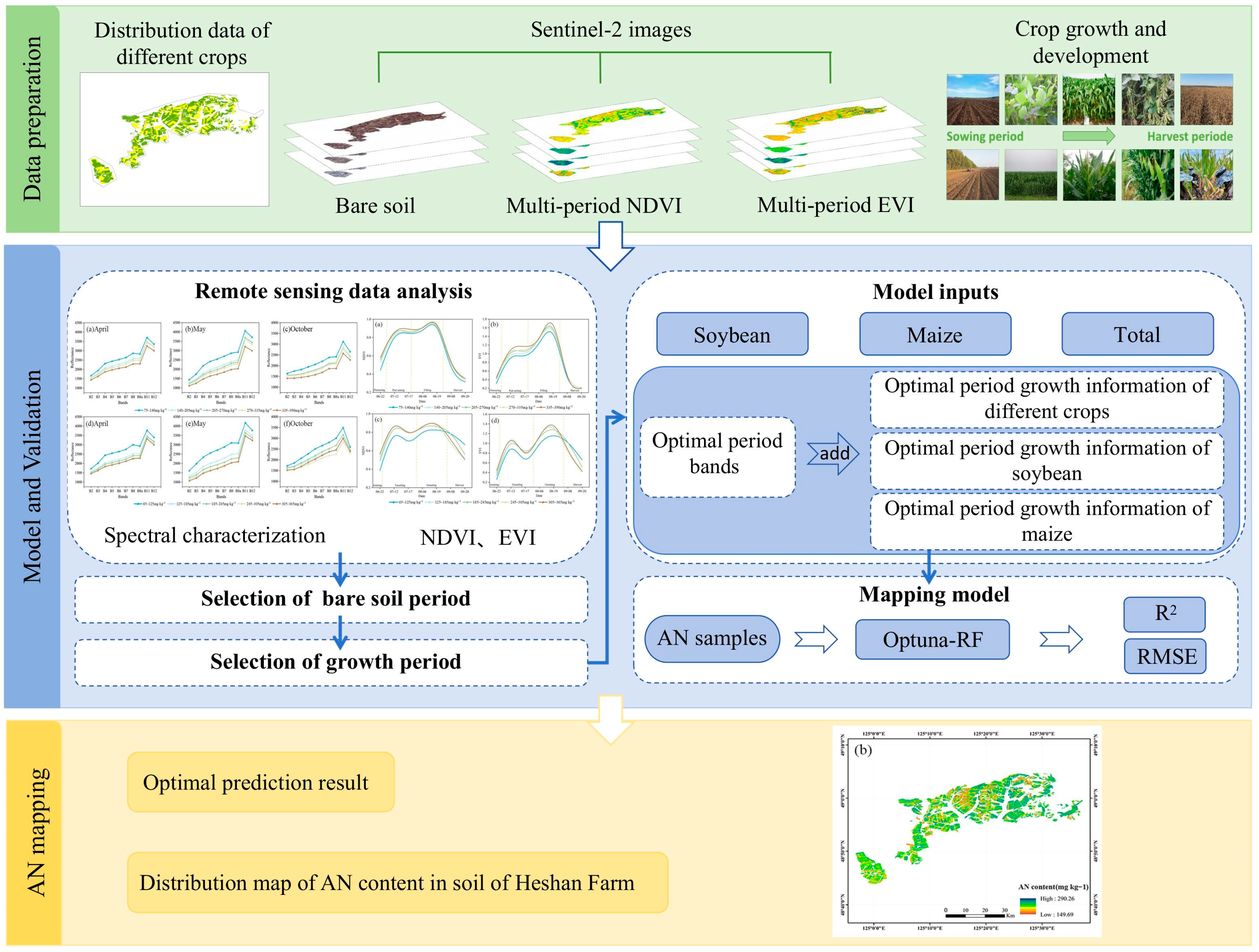
2.6. Technology Roadmap

This study is organized into three main parts: (1) Data Acquisition and Preprocessing: this section covers the acquisition and preprocessing of remote sensing images (April–October), as well as the extraction of multi-period crop growth information using NDVI and EVI time series data. (2) Analysis and Mapping: this section focuses on the selection and comparison of spectral features from soybean and maize plantations during different periods and the use of multi-period growth information to determine the optimal window period. Based on the comparison results, the optimal period growth information for soybean and maize plantations, as well as the combination of this information, was used to map the spatial distribution of soil AN content. (3) Evaluation of Mapping Accuracy: this section involves the mapping of soil AN distribution within the study area and the analysis of spatial variations in AN content. The specific technical workflow is illustrated in Figure 4.

3. Results

3.1. Remote Sensing Data with Different AN Contents

3.1.1. Spectral Character of Different AN Contents During the Bare Soil Period

The spectral reflectance of soils in Sentinel-2 satellite images exhibited significant differences across different time window periods and different soil AN content levels (Figure 5). The research has found that the spectral reflectance curves of soils with different AN contents in both soybean and maize plantations showed similar trends during the same time periods (April, May, and October). Specifically, the curves displayed a gradual increase in reflectance from B2 to B8, followed by a decline at B8a, peaking at B11. The higher the soil AN content, the lower the spectral reflectance; the spectral reflectance curves for different periods within the same plantation followed similar trends, though there were differences in specific values, particularly between the B4 and B8 bands. Notably, the spectral reflectance in areas with the lowest soil AN content was 18–67% higher than in areas with the highest AN content, especially in the B8 band, where the difference in reflectance between the two types of areas was most pronounced, ranging from 22% to 62%.

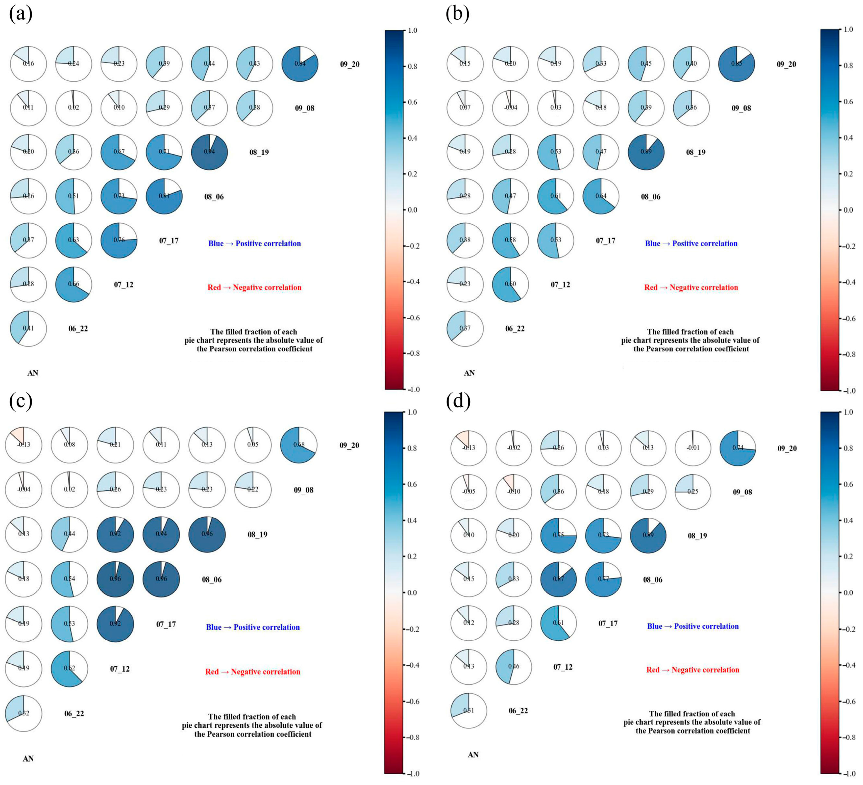
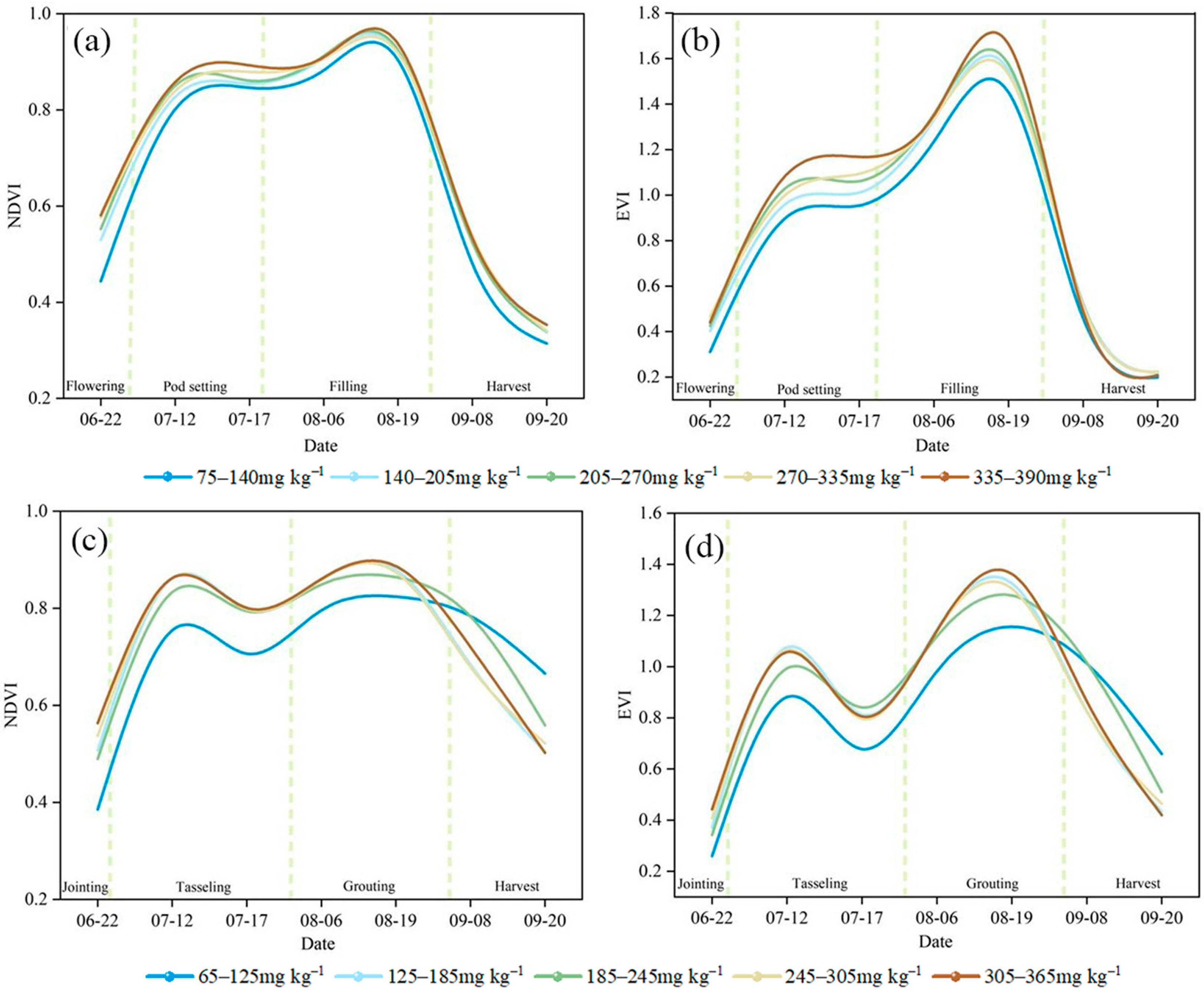
3.1.2. Differences in Growth of Different Crops

Based on the variability in the growth cycles of soybean and maize, their NDVI and EVI vegetation indices exhibited distinct trends throughout their growth periods (Figure 6). The NDVI and EVI values of soybean plantations showed a steadily increasing trend throughout the growth period (June, July, August, and September), whereas the NDVI and EVI values of maize plantations exhibited a fluctuating trend characterized by periods of “increase, then decrease, then increase.” This reflected the characteristics of different periods within the crop growth cycle: (i) in soybean plantations, NDVI and EVI values gradually increased during the flowering period from June to early July, slowed during the pod setting period in mid-July, peaked after the filling period in mid-August, and then rapidly declined as the harvest period approached in September; and (ii) in maize plantations, NDVI and EVI values gradually increased during the jointing period from June to early July, declined during the tasseling period in mid-July, peaked during the grouting period in mid-August, and then gradually declined in September as the harvest period approached.
This research found a significant correlation between crop growth status and ammonium nitrate content in soil. Specifically, areas with high AN content generally showed higher NDVI and EVI values than areas with low AN content, with the vegetation index values of areas with high AN content being 9–47% higher than those in areas with low AN content. This underscores the important role of AN supply in promoting healthy crop growth. This research has found that EVI is more effective than NDVI in reflecting differences in crop growth at different periods (Figure A1 in Appendix A). Specifically, the EVI of soybean varied from 37.989% to 42.502% between the pod setting and filling periods, while NDVI varied only from 5.045% to 10.112% during the same period. Similarly, the EVI of maize varied from 28.977% to 44.904% between the tasseling and grouting periods, compared to the NDVI’s range of 2.784% to 12.606%. Therefore, by monitoring crop growth conditions, soil status can be indirectly assessed. This approach mitigates the effect of instability in remote sensing data during the bare soil period. Effectively combining remote sensing data from both the bare soil and growth periods can significantly enhance the accuracy and reliability of soil AN content mapping.

3.2. AN Mapping Accuracy for Different Bare Soil Periods

Remote sensing images taken during different bare soil periods exhibited significant differences in accuracy when applied to soil AN mapping (Table 3). The research has found that the mapping accuracy in spring (April and May) was significantly better than that in fall (October) for both soybean and maize plantations; specifically, the average R2 values for spring mappings were 0.106 and 0.100 higher compared to fall, while the RMSE was reduced by 0.929% and 0.506%, respectively. These results indicate that spring image data offer higher accuracy and reliability for soil AN mapping; further analysis of the April and May data revealed that the difference in mapping accuracy between these two months was minimal, with the R2 difference ranging from 0.032 to 0.035, and the RMSE difference ranging from 0.159% to 0.461%. This suggests that mapping accuracy remained relatively stable between the two months, with April image data slightly outperforming May, as shown in the soybean plantations (R2 = 0.557, RMSE = 2.466%) and the maize plantations (R2 = 0.491, RMSE = 7.251%). Given the excellent performance of the April image data in soil AN mapping, this study used April image data as the base for subsequent soil AN mapping.

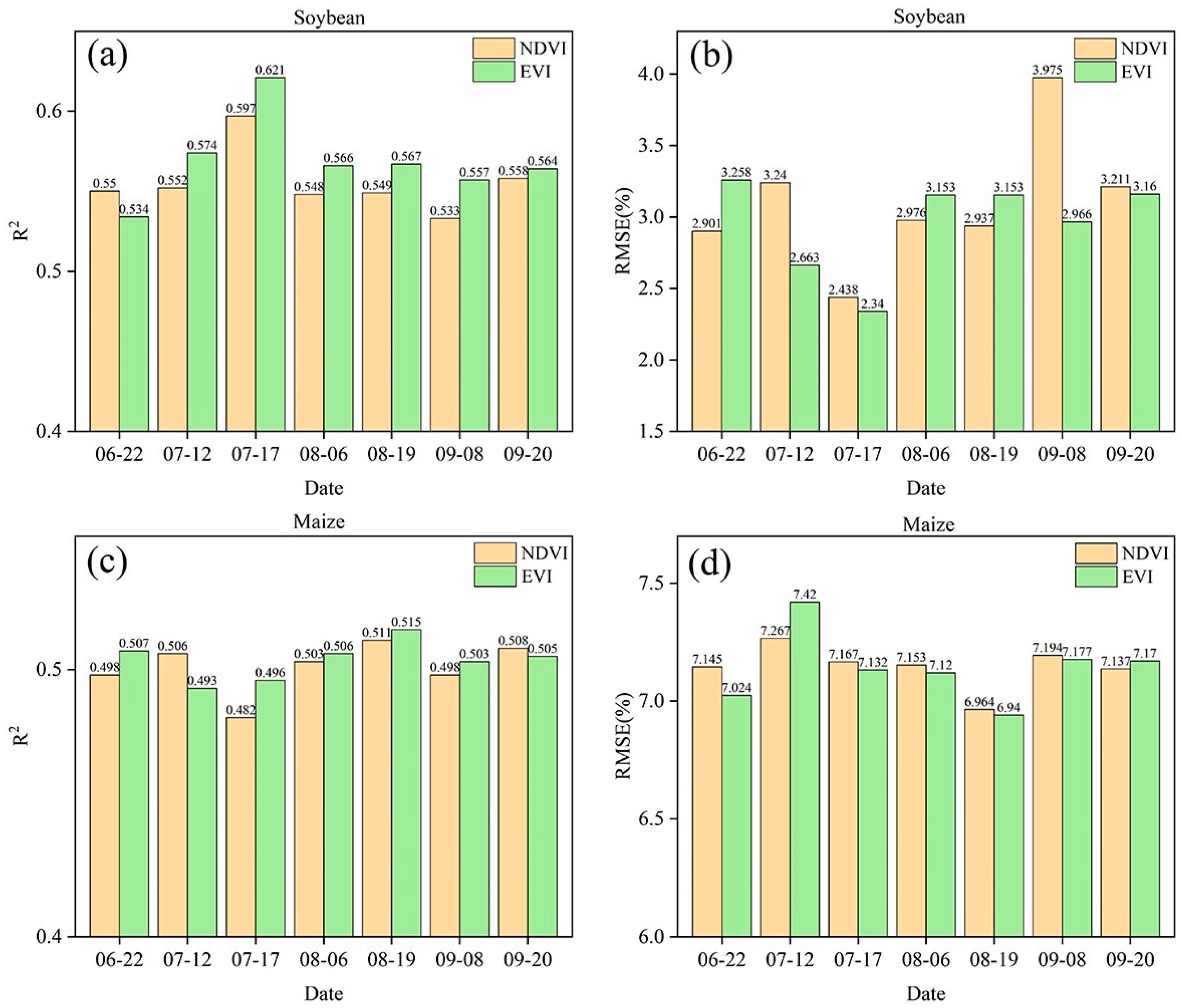
3.3. AN Mapping Accuracy by Introducing Information About Different Growth Periods

In this study, the effect of introducing crop-specific growth period information into soil AN mapping, based on the use of bare soil period images, was further investigated. The results demonstrated that integrating crop growth information can enhance the accuracy of soil AN mapping, although the impact of growth information varies across different crop types and growth periods (Figure 7). When different vegetation index data were introduced, it was found that crop-specific growth period EVI data were more beneficial for soil AN mapping compared to NDVI data. The R2 improved by 0.004–0.024 when EVI data were used, compared to NDVI data; when growth information of different growth periods was introduced, differences between soybean and maize plantations were observed. Specifically, for soybean plantations, the introduction of EVI data from the pod setting period resulted in the highest mapping accuracy, with an R2 of 0.621 and RMSE of 2.340%, which was a 0.064 improvement in R2 and a 0.126% reduction in RMSE compared to using bare soil period image data, and R2 increased by 0.024–0.088 compared with the introduction of growth information from other periods. For maize plantations, the introduction of EVI growth information at grouting period had the best effect, with an R2 of 0.515 and RMSE of 6.940%, in which R2 was 0.024 higher than that of using bare soil period image data, and increased by 0.004–0.033 compared with the introduction of growth information from other periods.
Although the EVI data at the pod setting and grouting periods were the most outstanding in improving the accuracy of soil AN mapping in soybean and maize plantations, the growth data at other growth periods also had a certain effect on the mapping accuracy, with R2 values ranging from 0.482 to 0.597. While these data effects were relatively stable, they still hold significant value in constructing a comprehensive and accurate soil AN mapping model. In summary, through categorical regression analysis for soybean and maize and their specific periods in the growth cycle, crop growth information can be more deeply understood and effectively utilized to optimize the mapping accuracy of soil AN.

3.4. Accuracy of Soil AN Mapping Based on Different Crop Types

This study aimed to evaluate the effectiveness of combining crop type and optimal growth period information in improving soil AN mapping accuracy, based on the significant differences in mapping accuracy between soybean and maize plantations and months (Table 4). The results showed that combining crop type and optimal growth period information effectively enhanced the accuracy of soil AN mapping. When only the bare soil period image was used for soil AN mapping, the R2 increased by 0.040 and 0.106, and the RMSE decreased by 0.222% and 5.007%. When crop growth information from these two periods and the optimal growth period information for soybean and maize plantations were introduced separately, the mapping method combining information of bare soil and optimal growth periods of specific crop types was the most effective. This method was significantly better than the method that introduced the optimal growth period information for both crop types as a whole. Specifically, compared to using only the bare soil image data, this method improved the R2 by 0.035 and reduced the RMSE by 0.504%; compared to the overall method of introducing the optimal period growth information of the two crop types, R2 increased by 0.047 and 0.101 and RMSE decreased by 0.929% and 1.759%. In conclusion, by combining the optimal period growth information of specific crop types, the influence of differences in crop growth cycles on mapping accuracy can be effectively reduced, leading to better mapping results.

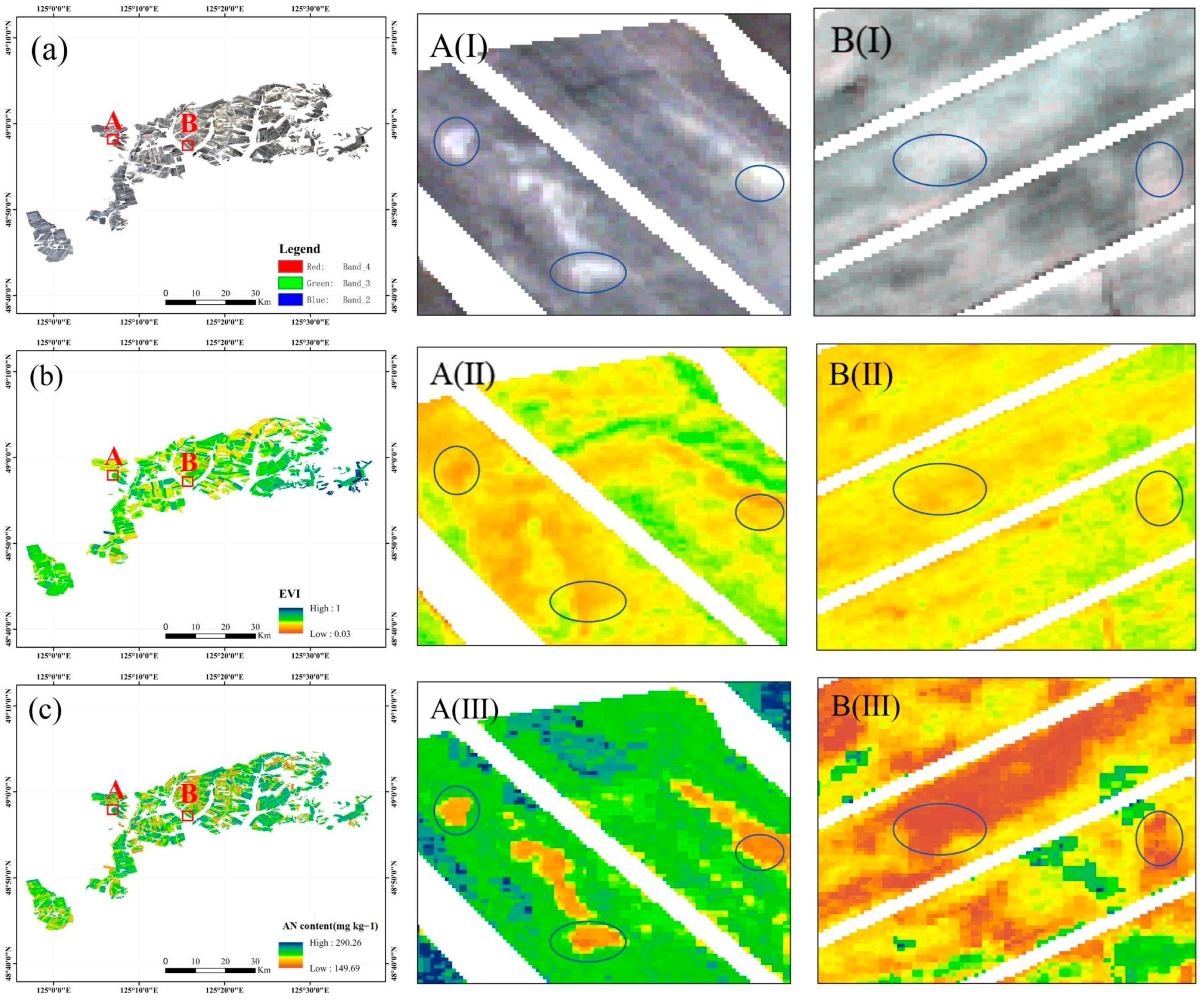
3.5. Spatial Distribution of Soil AN Content

The findings revealed that the spatial distribution of AN content in topsoil mapped based on the bare soil period image and the introduction of crop growth information exhibited similar patterns (Figure 8). High AN content values were predominantly concentrated in the northeast and southwest of the study area, while low values were mostly distributed in the central part of the study area, and a small amount of them were distributed in the mountainous cultivated areas in the west and east of the study area.
Among the different mapping approaches, the method incorporating the optimal growth period information for soybean and maize plantations performed slightly better than those based solely on the bare soil period image or those using growth information from 17 July and 19 August. These results showed accuracy improvements ranging from 5.863% to 19.021% compared to the other three methods. Although all four maps displayed similar general distribution patterns of soil AN content, differences were observed in local details. Compared to the mapping results based on bare soil period image data, the spatial variability of the mapping was more obvious with the introduction of the optimal period growth information of soybean and maize plantations, which improved the prediction of maximum and minimum values by 6.05 to 6.71 mg kg−1.
Furthermore, when compared with the results with the introduction of information on the growth of 17 July and 19 August, the method more effectively highlighted differences in soil AN content between cropping systems and provided a more detailed and accurate depiction of the soil AN content patterns. In this way, the mean soil AN content for soybean and maize plantations was 224.206 mg kg−1 and 234.558 mg kg−1, respectively, while for the two periods, the mean soil AN content for soybean and maize plantations was 225.383 mg kg−1, 231.176 mg kg−1, and 224.936 mg kg−1, 233.811 mg kg−1, respectively. The mapping method proposed in this paper is based on images of the bare soil period and introduces information on the optimal growth period of soybean and maize plantations; it not only provides strong support for the in-depth understanding of the characteristics of soil resources but also offers a scientific basis for precision agriculture practices.

4. Discussion

4.1. Impact of Introducing Growth Information on AN Content Mapping

Traditional methods of soil AN mapping primarily rely on randomly selected bare soil period images as the main data source. However, the mapping accuracy of these bare soil period images varied significantly between different months [53]. Specifically, the mapping accuracy of image data from the bare soil period in spring was notably higher than in the fall, with the highest single-cycle mapping accuracy observed for April images (Table 3). This finding contrasts with the results of Luo et al. [54], which may be attributed to differences in the sowing times of crops in various regions, leading to mismatches between image acquisition and the timing of soil sample collection in the field. However, relying solely on bare soil period images cannot fully capture the dynamic interaction between crops and soil. The growth status of crops can, to some extent, reflect the fertility level of the soil. Therefore, the introduction of crop growth information provides dynamic features for soil AN mapping. By introducing vegetation index information of soybean and maize plantations at different growth periods, the cumulative effect of crops on soil nutrient absorption can be more effectively captured, thus providing a more comprehensive feature description for spatial distribution modeling of soil AN [55]. NDVI and EVI, as commonly used vegetation indices, can not only effectively reflect the growth status of crops, but also indirectly reveal the supply capacity of soil AN, providing an important temporal remote sensing basis for soil attribute modeling [56].
In this study, by analyzing the effects of different crop types and growth periods on the accuracy of AN mapping with images of the bare soil period combined with the growth information of crop growth periods, it was found that this information had different effects on the accuracy of soil AN mapping. The highest mapping accuracy was found in soybean and maize plantations when EVI data were introduced at the pod setting and grouting periods, respectively, and the effect of growth data at other periods was relatively stable although it had a certain effect on the accuracy of soil AN mapping, which may be attributed to the fact that canopy structural features and spectral features of crops at specific growth periods are more similar. The growth information of the two periods can effectively characterize the differences in crop growth under different AN contents [57,58].

4.2. Combining the Advantages of Different Crop Types

In this study, considering the significant differences in planting systems, tillage methods, and growth cycles between soybean and maize, as well as their different impacts on the accuracy of soil AN mapping, we divided the study area into two parts, soybean and maize, and compared and analyzed the differences in changes in soil AN content between these two crops after introducing growth information at different growth periods. The results revealed significant variability in the mapping accuracy of soil AN content across plantations of soybean and maize when growth information was introduced. Specifically, the overall regression method, which combined crop types with their optimal growth period information, demonstrated better mapping accuracy compared to the method of classifying regression for each crop type individually, with an increase in R2 of 0.011 and 0.117, respectively. Compared with the method of integrating the introduction of the optimal period growth information of the two crop types, R2 improved by 0.047 and 0.101, respectively (Table 4).
This phenomenon may be closely related to the diversity of crop types and significant differences in the growth cycles of different crops in the study area [59,60] (Figure 2). The classifying regression analysis of soybean and maize plantations can more effectively capture the regional characteristics of different crop types, make up for the shortcomings of a single model in dealing with multiple types of crops, and further explore the impact of growth information on soil AN mapping. On this basis, combining the growth information of two crop types and their optimal growth periods can effectively reduce the interference of different crop growth information on soil AN mapping (Figure 9), thereby improving the mapping accuracy of soil AN content and reducing errors.
The soil AN mapping method proposed in this article, which combines the growth information of two crop types, soybean and maize, provides a new perspective and technical path for future soil attribute mapping research. This method can not only reveal the dynamic relationship between crops and soil but also effectively reduce the impact of regional differences and improve the accuracy of soil attribute mapping. This modeling strategy, which comprehensively considers crop types and their growth dynamics, provides a solid scientific basis and technical support for optimizing fertilization management, efficient resource utilization, and sustainable environmental development in precision agriculture.

4.3. Limitations and Perspectives

In this study, we evaluated the reflectance of different AN contents in images from different bare soil periods, analyzed the relationship between AN contents and vegetation productivity across soybean and maize plantations, and compared the differences in the accuracy of soil AN mapping before and after the introduction of crop growth information in different periods, which provided a new idea for the mapping of soil AN. However, this study also has some limitations. Firstly, this study only utilized bare soil period images combined with crop growth information to estimate the spatial distribution of AN in the study area. However, the distribution of AN content is also influenced by various factors, including geographical location, environmental factors, and changes in management practices. For example, different tillage methods in various regions may lead to significant differences in soil nutrient content [61]. Therefore, future research will introduce multi-source data to more comprehensively estimate AN content and improve the accuracy of the model [53].
Secondly, this study utilized only the decision tree-based Random Forest (RF) algorithm to map the spatial distribution of soil AN. In recent years, more and more studies have begun to explore the application of other machine learning and deep learning methods (e.g., convolutional neural networks, CNN) to realize the soil digital mapping work [26,62], but this often requires more soil sample sizes and explanatory variables to obtain better training results. Given this, existing machine learning algorithms will be utilized in future research to systematically compare emerging AI techniques and explore efficient algorithms that are best suited for diverse application scenarios.

5. Conclusions

This study comprehensively considers the differences in crop types, remote sensing data acquisition time, and crop growth status. Based on bare soil images, combined with soybean and maize plantations and their optimal period growth information, an effective new method for spatial mapping of soil available nitrogen was constructed. The research results indicate that (1) the introduction of crop growth information can improve the accuracy of AN mapping, especially when referring to EVI growth information of the soybean pod setting period and maize growing period. The mapping accuracy of AN can reach 0.621 and 0.515, which is 0.024–0.064 higher than the R2 when using bare soil image data. (2) Combining the optimal period growth information of two crop types, soybean and maize, not only improves the accuracy of soil AN mapping, but also effectively reduces the impact of crop differences. The method improves the mapping accuracy by 0.047–0.101 compared with the overall introduction of the optimal period growth information of the two crop types. (3) Although bare soil images can directly describe the surface state of soil, there are differences in the accuracy of using band information from different periods for soil AN mapping. The mapping accuracy of bare soil image data in spring is significantly better than that in autumn, with April being the best time window for bare soil in the study area. This study not only deepens our understanding of the spatial distribution of soil AN but also provides a scientific basis for the research and development of precision agriculture. In future research, it is necessary to explore in depth how to more effectively utilize crop growth information from different periods and regions to optimize agricultural management and resource allocation, thereby promoting sustainable agricultural development.

Author Contributions

Conceptualization, X.Z. (Xinle Zhang) and H.L.; data curation, Y.M. and Y.W.; formal analysis, Y.M., S.M. and Y.W.; methodology, X.Z. (Xinle Zhang), Y.W. and Y.M.; project administration, X.Z. (Xinle Zhang) and H.L.; software, C.Q., L.C. and X.Z. (Xiaomeng Zhu); writing—original draft, X.Z. (Xinle Zhang) and Y.M.; writing—review and editing, X.Z. (Xinle Zhang) and Y.W. All authors have read and agreed to the published version of the manuscript.

Funding

This research was supported by the National Key R&D Program of China (2024YFD1501100), the National Key R&D Program of China (2021YFD1500100), the Science and Technology Development Plan Project of Jilin Province, China (20240101043JC), and the Jilin Agricultural University Introduction of Talents Project (No. 202020010).

Data Availability Statement

Data are not available due to privacy restrictions; please contact the corresponding author.

Acknowledgments

We thank the National Earth System Science Data Center for providing geographic information data.

Conflicts of Interest

The authors declare no conflicts of interest.

Appendix A

Figure A1. The correlation between variables. Soybean Plantations: (a) NDVI; (b) EVI. Maize Plantations: (c) NDVI; (d) EVI.
Agriculture 15 01531 g0a1

References

  1. Bao, S.D. Soil Agrochemical Analysis; China Agriculture Press: Beijing, China, 2005. [Google Scholar]
  2. Vitousek, P.M.; Howarth, R.W. Nitrogen Limitation on Land and in the Sea: How Can It Occur? Biogeochemistry 1991, 13, 87–115. [Google Scholar] [CrossRef]
  3. Leghari, S.J.; Wahocho, N.A.; Laghari, G.M.; Laghari, A.H.; Bhabhan, G.M.; Talpur, K.H. Role of nitrogen for plant growth and development: A review. Adv. Environ. Biol. 2016, 10, 209–219. [Google Scholar]
  4. Pramanick, B.; Choudhary, S.; Kumar, M.; Singh, S.K.; Jha, R.K.; Singh, S.K. Can site-specific nutrient management improve the productivity and resource use efficiency of climate-resilient finger millet in calcareous soils in India? Heliyon 2024, 10, e32774. [Google Scholar] [CrossRef] [PubMed]
  5. Zhou, T.; Geng, Y.; Chen, J.; Pan, J.; Haase, D.; Lausch, A. High-Resolution Digital Mapping of Soil Organic Carbon and Soil Total Nitrogen Using DEM Derivatives, Sentinel-1 and Sentinel-2 Data Based on Machine Learning Algorithms. Sci. Total Environ. 2020, 729, 138244. [Google Scholar] [CrossRef] [PubMed]
  6. Lamichhane, S.; Kumar, L.; Wilson, B. Digital Soil Mapping Algorithms and Covariates for Soil Organic Carbon Mapping and Their Implications: A Review. Geoderma 2019, 352, 395–413. [Google Scholar] [CrossRef]
  7. Loiseau, T.; Chen, S.; Mulder, V.L.; Dobarco, M.R.; Richer-de-Forges, A.C.; Lehmann, S.; Arrouays, D. Satellite Data Integration for Soil Clay Content Modelling at a National Scale. Int. J. Appl. Earth Obs. Geoinf. 2019, 82, 101905. [Google Scholar] [CrossRef]
  8. Cai, W.; He, N.; Li, M.; Xu, L.; Wang, L.; Zhu, J.; Sun, O.J. Carbon Sequestration of Chinese Forests from 2010 to 2060: Spatiotemporal Dynamics and Its Regulatory Strategies. Sci. Bull. 2022, 67, 836–843. [Google Scholar] [CrossRef] [PubMed]
  9. Li, Y.; Ma, J.; Li, Y.; Jia, Q.; Shen, X.; Xia, X. Spatiotemporal Variations in the Soil Quality of Agricultural Land and Its Drivers in China from 1980 to 2018. Sci. Total Environ. 2023, 892, 164649. [Google Scholar] [CrossRef] [PubMed]
  10. Meng, X.; Bao, Y.; Luo, C.; Zhang, X.; Liu, H. SOC Content of Global Mollisols at a 30 m Spatial Resolution from 1984 to 2021 Generated by the Novel ML-CNN Prediction Model. Remote Sens. Environ. 2024, 300, 113911. [Google Scholar] [CrossRef]
  11. Wang, H.; Wang, J.; Ma, R.; Zhou, W. Soil nutrients inversion in open-pit coal mine reclamation area of Loess Plateau, China: A study based on ZhuHai-1 hyperspectral remote sensing. Land Degrad. Dev. 2024, 35, 5210–5223. [Google Scholar] [CrossRef]
  12. Lachgar, A.; Mulla, D.J.; Adamchuk, V. Implementation of Proximal and Remote Soil Sensing, Data Fusion and Machine Learning to Improve Phosphorus Spatial Prediction for Farms in Ontario, Canada. Agronomy 2024, 14, 693. [Google Scholar] [CrossRef]
  13. Yang, L.; He, X.; Shen, F.; Zhou, C.; Zhu, A.X.; Gao, B.; Li, M. Improving Prediction of Soil Organic Carbon Content in Croplands Using Phenological Parameters Extracted from NDVI Time Series Data. Soil Tillage Res. 2020, 196, 104465. [Google Scholar] [CrossRef]
  14. Wu, Z.; Liu, Y.; Han, Y.; Zhou, J.; Liu, J.; Wu, J. Mapping Farmland Soil Organic Carbon Density in Plains with Combined Cropping System Extracted from NDVI Time-Series Data. Sci. Total Environ. 2021, 754, 142120. [Google Scholar] [CrossRef] [PubMed]
  15. Yang, C.; Yang, L.; Zhang, L.; Zhou, C. Soil Organic Matter Mapping Using INLA-SPDE with Remote Sensing Based Soil Moisture Indices and Fourier Transforms Decomposed Variables. Geoderma 2023, 437, 116571. [Google Scholar] [CrossRef]
  16. Mutanga, O.; Masenyama, A.; Sibanda, M. Spectral Saturation in the Remote Sensing of High-Density Vegetation Traits: A Systematic Review of Progress, Challenges, and Prospects. ISPRS J. Photogramm. Remote Sens. 2023, 198, 297–309. [Google Scholar] [CrossRef]
  17. Kowalski, K.; Senf, C.; Hostert, P.; Pflugmacher, D. Characterizing Spring Phenology of Temperate Broadleaf Forests Using Landsat and Sentinel-2 Time Series. Int. J. Appl. Earth Obs. Geoinf. 2020, 92, 102172. [Google Scholar] [CrossRef]
  18. Liu, L.; Xiao, X.; Qin, Y.; Wang, J.; Xu, X.; Hu, Y.; Qiao, Z. Mapping Cropping Intensity in China Using Time Series Landsat and Sentinel-2 Images and Google Earth Engine. Remote Sens. Environ. 2020, 239, 111624. [Google Scholar] [CrossRef]
  19. Pan, L.; Xia, H.; Zhao, X.; Guo, Y.; Qin, Y. Mapping Winter Crops Using a Phenology Algorithm, Time-Series Sentinel-2 and Landsat-7/8 Images, and Google Earth Engine. Remote Sens. 2021, 13, 2510. [Google Scholar] [CrossRef]
  20. Lobell, D.B.; Lesch, S.M.; Corwin, D.L.; Ulmer, M.G.; Anderson, K.A.; Potts, D.J.; Baltes, M.J. Regional-Scale Assessment of Soil Salinity in the Red River Valley Using Multi-Year MODIS EVI and NDVI. J. Environ. Qual. 2010, 39, 35–41. [Google Scholar] [CrossRef] [PubMed]
  21. Hamzehpour, N.; Shafizadeh-Moghadam, H.; Valavi, R. Exploring the Driving Forces and Digital Mapping of Soil Organic Carbon Using Remote Sensing and Soil Texture. Catena 2019, 182, 104141. [Google Scholar] [CrossRef]
  22. Yang, L.; Song, M.; Zhu, A.X.; Qin, C.; Zhou, C.; Qi, F.; Gao, B. Predicting Soil Organic Carbon Content in Croplands Using Crop Rotation and Fourier Transform Decomposed Variables. Geoderma 2019, 340, 289–302. [Google Scholar] [CrossRef]
  23. Reddy, P.P. Sustainable Intensification of Crop Production. In Sustainable Intensification of Crop Production; Springer: Singapore, 2016; pp. 143–154. [Google Scholar]
  24. Chen, S.; Yao, H.; Zhang, X. Nitrous Oxide Emission from Cropland and Its Driving Factors under Different Crop Rotations. Sci. Agric. Sin. 2005, 38, 2053–2060. [Google Scholar]
  25. You, L.; Ros, G.H.; Chen, Y.; Shao, Q.; Young, M.D.; Zhang, F.; De Vries, W. Global Mean Nitrogen Recovery Efficiency in Croplands Can Be Enhanced by Optimal Nutrient, Crop and Soil Management Practices. Nat. Commun. 2023, 14, 5747. [Google Scholar] [CrossRef] [PubMed]
  26. Li, H.; Ju, W.; Song, Y.; Cao, Y.; Yang, W.; Li, M. Soil organic matter content prediction based on two-branch convolutional neural network combining image and spectral features. Comput. Electron. Agric. 2024, 217, 108561. [Google Scholar]
  27. Lu, D.; Chen, Q.; Wang, G.; Moran, E.; Batistella, M.; Zhang, M.; Saah, D. Aboveground Forest Biomass Estimation with Landsat and LiDAR Data and Uncertainty Analysis of the Estimates. Int. J. For. Res. 2012, 2012, 436537. [Google Scholar] [CrossRef]
  28. Gregoire, T.G.; Næsset, E.; McRoberts, R.E.; Ståhl, G.; Andersen, H.E.; Gobakken, T.; Nelson, R. Statistical Rigor in LiDAR-Assisted Estimation of Aboveground Forest Biomass. Remote Sens. Environ. 2016, 173, 98–108. [Google Scholar] [CrossRef]
  29. Geng, J.; Tan, Q.; Lv, J.; Fang, H. Assessing spatial variations in soil organic carbon and C:N ratio in Northeast China’s black soil region: Insights from Landsat-9 satellite and crop growth information. Soil Tillage Res. 2024, 235, 105897. [Google Scholar] [CrossRef]
  30. Deiss, L.; Margenot, A.J.; Culman, S.W.; Demyan, M.S. Tuning Support Vector Machines Regression Models Improves Prediction Accuracy of Soil Properties in MIR Spectroscopy. Geoderma 2020, 365, 114227. [Google Scholar] [CrossRef]
  31. Jia, Y.; Jin, S.; Savi, P.; Yan, Q.; Li, W. Modeling and Theoretical Analysis of GNSS-R Soil Moisture Retrieval Based on the Random Forest and Support Vector Machine Learning Approach. Remote Sens. 2020, 12, 3679. [Google Scholar] [CrossRef]
  32. Mondal, B.P.; Sahoo, R.N.; Ahmed, N.; Singh, R.K.; Das, B.; Mridha, N.; Gakhar, S. Rapid prediction of soil available sulphur using visible near-infrared reflectance spectroscopy. Indian J. Agric. Sci. 2021, 91, 1328–1332. [Google Scholar] [CrossRef]
  33. Camargo, L.A.; do Amaral, L.R.; dos Reis, A.A.; Brasco, T.L.; Magalhães, P.S.G. Improving Soil Organic Carbon Mapping with a Field-Specific Calibration Approach through Diffuse Reflectance Spectroscopy and Machine Learning Algorithms. Soil Use Manag. 2022, 38, 292–303. [Google Scholar] [CrossRef]
  34. Akiba, T.; Sano, S.; Yanase, T.; Ohta, T.; Koyama, M. Optuna: A Next-Generation Hyperparameter Optimization Framework. In Proceedings of the 25th ACM SIGKDD International Conference on Knowledge Discovery & Data Mining, Anchorage, AK, USA, 4–8 July 2019; pp. 2623–2631. [Google Scholar]
  35. Almarzooq, H.; bin Waheed, U. Automating Hyperparameter Optimization in Geophysics with Optuna: A Comparative Study. Geophys. Prospect. 2024, 72, 1778–1788. [Google Scholar] [CrossRef]
  36. Yu, Y.; Zhang, K.; Liu, L.; Ma, Q.; Luo, J. Estimating Long-Term Erosion and Sedimentation Rate on Farmland Using Magnetic Susceptibility in Northeast China. Soil Till. Res. 2019, 187, 41–49. [Google Scholar] [CrossRef]
  37. Claverie, M.; Ju, J.; Masek, J.G.; Dungan, J.L.; Vermote, E.F.; Roger, J.C.; Justice, C. The Harmonized Landsat and Sentinel-2 Surface Reflectance Data Set. Remote Sens. Environ. 2018, 219, 145–161. [Google Scholar] [CrossRef]
  38. Wu, B.; Sun, Y.; Wang, G.; Wang, J. Spatial Variability of Available Nitrogen in Soil and Its Response to Sampling Intervals in the Southern Breeding Base of Maize. Guangdong Agric. Sci. 2023, 50, 66–74. [Google Scholar]
  39. Peng, D.; Wu, C.; Li, C.; Zhang, X.; Liu, Z.; Ye, H.; Fang, B. Spring Green-Up Phenology Products Derived from MODIS NDVI and EVI: Intercomparison, Interpretation and Validation Using National Phenology Network and AmeriFlux Observations. Ecol. Indic. 2017, 77, 323–336. [Google Scholar] [CrossRef]
  40. Testa, S.; Soudani, K.; Boschetti, L.; Mondino, E.B. MODIS-Derived EVI, NDVI and WDRVI Time Series to Estimate Phenological Metrics in French Deciduous Forests. Int. J. Appl. Earth Obs. Geoinf. 2018, 64, 132–144. [Google Scholar] [CrossRef]
  41. Gu, Y.; Wylie, B.K.; Howard, D.M.; Phuyal, K.P.; Ji, L. NDVI Saturation Adjustment: A New Approach for Improving Cropland Performance Estimates in the Greater Platte River Basin, USA. Ecol. Indic. 2013, 30, 1–6. [Google Scholar] [CrossRef]
  42. Gao, S.; Zhong, R.; Yan, K.; Ma, X.; Chen, X.; Pu, J.; Myneni, R.B. Evaluating the Saturation Effect of Vegetation Indices in Forests Using 3D Radiative Transfer Simulations and Satellite Observations. Remote Sens. Environ. 2023, 295, 113665. [Google Scholar] [CrossRef]
  43. Cao, R.; Chen, Y.; Shen, M.; Chen, J.; Zhou, J.; Wang, C.; Yang, W. A Simple Method to Improve the Quality of NDVI Time-Series Data by Integrating Spatiotemporal Information with the Savitzky-Golay Filter. Remote Sens. Environ. 2018, 217, 244–257. [Google Scholar] [CrossRef]
  44. Cao, R.; Chen, J.; Shen, M.; Tang, Y. An Improved Logistic Method for Detecting Spring Vegetation Phenology in Grasslands from MODIS EVI Time-Series Data. Agric. For. Meteorol. 2015, 200, 9–20. [Google Scholar] [CrossRef]
  45. Sen, Z.; Xia, L.; Ge-Ge, N.; Yu-Rong, L.; Ya-Ting, S.; Yan-Qin, T.; Yu-Juan, Z. Estimation of soil organic matter in coastal wetlands by SVM and BP based on hyperspectral remote sensing. Spectrosc. Spectr. Anal. 2020, 40, 556–561. [Google Scholar]
  46. Lu, B.; Liu, N.; Li, H.; Yang, K.; Hu, C.; Wang, X.; Tang, X. Quantitative determination and characteristic wavelength selection of available nitrogen in coco-peat by NIR spectroscopy. Soil Tillage Res. 2019, 191, 266–274. [Google Scholar] [CrossRef]
  47. Wang, Y.; Xue, Z.; Chen, J.; Chen, G. Spatio-Temporal Analysis of Phenology in Yangtze River Delta Based on MODIS NDVI Time Series from 2001 to 2015. Front. Earth Sci. 2019, 13, 92–110. [Google Scholar] [CrossRef]
  48. Genuer, R.; Poggi, J.M. Random Forests. In Random Forests with R; Springer International Publishing: Cham, Switzerland, 2020; pp. 33–55. [Google Scholar]
  49. Hengl, T.; Nussbaum, M.; Wright, M.N.; Heuvelink, G.B.M.; Gräler, B. Random Forest as a Generic Framework for Predictive Modeling of Spatial and Spatio-Temporal Variables. PeerJ 2018, 6, e5518. [Google Scholar] [CrossRef] [PubMed]
  50. Hu, B.; Xie, M.; Zhou, Y.; Chen, S.; Zhou, Y.; Ni, H.; Shi, Z. A High-Resolution Map of Soil Organic Carbon in Cropland of Southern China. Catena 2024, 237, 107813. [Google Scholar] [CrossRef]
  51. Krivorotko, O.; Sosnovskaia, M.; Vashchenko, I.; Kerr, C.; Lesnic, D. Agent-based modeling of COVID-19 outbreaks for New York state and UK: Parameter identification algorithm. Infect. Dis. Model. 2022, 7, 30–44. [Google Scholar] [CrossRef] [PubMed]
  52. Suryadi, M.K.; Herteno, R.; Saputro, S.W.; Faisal, M.R.; Nugroho, R.A. Comparative Study of Various Hyperparameter Tuning on Random Forest Classification with SMOTE and Feature Selection Using Genetic Algorithm in Software Defect Prediction. J. Electron. Electromed. Eng. Med. Inform. 2024, 6, 137–147. [Google Scholar] [CrossRef]
  53. Zhang, Y.; Luo, C.; Zhang, W.; Wu, Z.; Zang, D. Mapping Soil Organic Matter in Black Soil Cropland Areas Using Remote Sensing and Environmental Covariates. Agriculture 2025, 15, 339. [Google Scholar] [CrossRef]
  54. Luo, C.; Zhang, X.; Wang, Y.; Men, Z.; Liu, H. Regional Soil Organic Matter Mapping Models Based on the Optimal Time Window, Feature Selection Algorithm and Google Earth Engine. Soil Tillage Res. 2022, 219, 105325. [Google Scholar] [CrossRef]
  55. Wolkowski, R.P. Relationship Between Wheel-Traffic-Induced Soil Compaction, Nutrient Availability, and Crop Growth: A Review. J. Prod. Agric. 1990, 3, 460–469. [Google Scholar] [CrossRef]
  56. Abishek, R.; Santhi, R.; Maragatham, S.; Venkatachalam, S.R.; Uma, D.; Lakshmanan, A. Response of Hybrid Castor under Different Fertility Gradient: Correlation Between Castor Yield and Normalized Difference Vegetation Index (NDVI) under Inductive Cum Targeted Yield Model on an Alfisol. Commun. Soil Sci. Plant Anal. 2023, 54, 1816–1831. [Google Scholar] [CrossRef]
  57. Fu, Z.; Ciais, P.; Wigneron, J.P.; Gentine, P.; Feldman, A.F.; Makowski, D.; Smith, W.K. Global Critical Soil Moisture Thresholds of Plant Water Stress. Nat. Commun. 2024, 15, 4826. [Google Scholar] [CrossRef] [PubMed]
  58. Kern, J.S. Geographic Patterns of Soil Water-Holding Capacity in the Contiguous United States. Soil Sci. Soc. Am. J. 1995, 59, 1126–1133. [Google Scholar] [CrossRef]
  59. Minoli, S.; Egli, D.B.; Rolinski, S.; Müller, C. Modelling Cropping Periods of Grain Crops at the Global Scale. Glob. Planet. Change 2019, 174, 35–46. [Google Scholar] [CrossRef]
  60. Minoli, S.; Jägermeyr, J.; Asseng, S.; Urfels, A.; Müller, C. Global Crop Yields Can Be Lifted by Timely Adaptation of Growing Periods to Climate Change. Nat. Commun. 2022, 13, 7079. [Google Scholar] [CrossRef] [PubMed]
  61. Ren, X.X.; Cai, T.J.; Wang, X.F. Effects of Vegetation Restoration Models on Soil Nutrients in an Abandoned Quarry. J. Beijing For. Univ. 2010, 32, 151–154. [Google Scholar]
  62. Zhong, L.; Guo, X.; Ding, M.; Ye, Y.; Zhu, Q.; Guo, J.; Zeng, X. Spatial Mapping of Topsoil Total Nitrogen in Mountainous and Hilly Areas of Southern China Using a Continuous Convolution Neural Network. Catena 2023, 229, 107228. [Google Scholar] [CrossRef]
Figure 1. Overview of the study area. (a) Location map of the study area, (b) Sentinel-2 multispectral image and location of sampling points in the study area, and (c) distribution of planting structures in the study area.
Agriculture 15 01531 g001
Figure 2. Fertility period of major crops in the study area.
Agriculture 15 01531 g002
Figure 3. Working diagram of Optuna algorithm.
Agriculture 15 01531 g003
Figure 4. Technology roadmap for mapping soil AN content.
Agriculture 15 01531 g004
Figure 5. Soil spectral reflectance of Sentinel-2 satellite for different crop bare soil periods ((ac) for soybean plantations and (df) for maize plantations).
Agriculture 15 01531 g005
Figure 6. (a,b) NDVI and EVI time series curves for soybean plantations; (c,d) NDVI and EVI time series curves for maize plantations.
Agriculture 15 01531 g006
Figure 7. AN mapping accuracy of soybean and maize plantations based on remote sensing imagery, introducing growth information at different growth periods. (a,b) Soybean plantations, (c,d) maize plantations.
Agriculture 15 01531 g007
Figure 8. Soil AN content mapping results based on the Optuna-RF model. (a) Spatial distribution of soil AN content based on bare soil period images, (b) spatial distribution of soil AN content introducing optimal period growth information of soybean and maize plantations, (c) spatial distribution of soil AN content introducing information on the growth of 17 July, and (d) spatial distribution of soil AN content introducing information on the growth of 19 August.
Agriculture 15 01531 g008
Figure 9. Detailed comparative results of synthetic images of bare soil period and growth information. (a) A single image on 11 April 2023, (b) combining EVI imagery of the crop’s optimal growth period, and (c) spatial distribution of AN in 2023. (A(I),B(I)) Local zoom images of a single image on 11 April 2023. (A(II),B(II)) Local zoom images of EVI images combined with the optimal growth period of crops. (A(III),B(III)) Local zoom images of spatial distribution of AN in 2023.
Agriculture 15 01531 g009
Table 1. Sensor parameters.
BandCentral Wavelength (nm)Bandwidth
(nm)
Spatial Resolution
(m)
B24906510
B35603510
B46653010
B57051520
B67401520
B77832020
B884211510
B8a8652020
B1116109020
B12219018020
Table 2. Statistical description of AN content (0–20 cm).
ZoneNMin
(mg kg−1)
Max
(mg kg−1)
Mean
(mg kg−1)
SDCV (%)
Total18865.81387.10213.8561.1628.60
Soybean12976.65387.10211.1760.4728.64
Maize5965.81357.68219.7662.8428.60
Note: Total represents the total data; Depth represents the depth of soil sampling; N represents the number of sampling points; Min represents the minimum value; Max represents the maximum value; SD represents the standard deviation; CV represents the coefficient of variation.
Table 3. Soil AN mapping accuracy for different crop types based on different months of Sentinel-2 imagery.
ZoneMonthR2RMSE (%)
SoybeanApril0.5572.466
May0.5222.927
October0.4343.625
MaizeApril0.4917.251
May0.4597.410
October0.3757.836
Table 4. Soil AN mapping accuracy combining crop type and growth information.
ZoneInput VariableR2RMSE (%)
SoybeanBands0.5572.466
Bands + EVI7170.6212.340
MaizeBands0.4917.251
Bands + EVI8190.5156.940
TotalBands0.5972.244
Bands + EVI7170.5852.669
Bands + EVI8190.5313.499
Bands + EVIc0.6321.740
Note: Bands: April remote sensing imagery during bare soil period; EVIc: 17 July 2023 soybean crop growth information combined with 19 August 2023 maize crop growth information.
Disclaimer/Publisher’s Note: The statements, opinions and data contained in all publications are solely those of the individual author(s) and contributor(s) and not of MDPI and/or the editor(s). MDPI and/or the editor(s) disclaim responsibility for any injury to people or property resulting from any ideas, methods, instructions or products referred to in the content.

