

Growth Stages Discrimination of Multi-Cultivar Navel Oranges Using the Fusion of Near-Infrared Hyperspectral Imaging and Machine Vision with Deep Learning


Abstract
1. Introduction
2. Materials and Methods
2.1. Samples
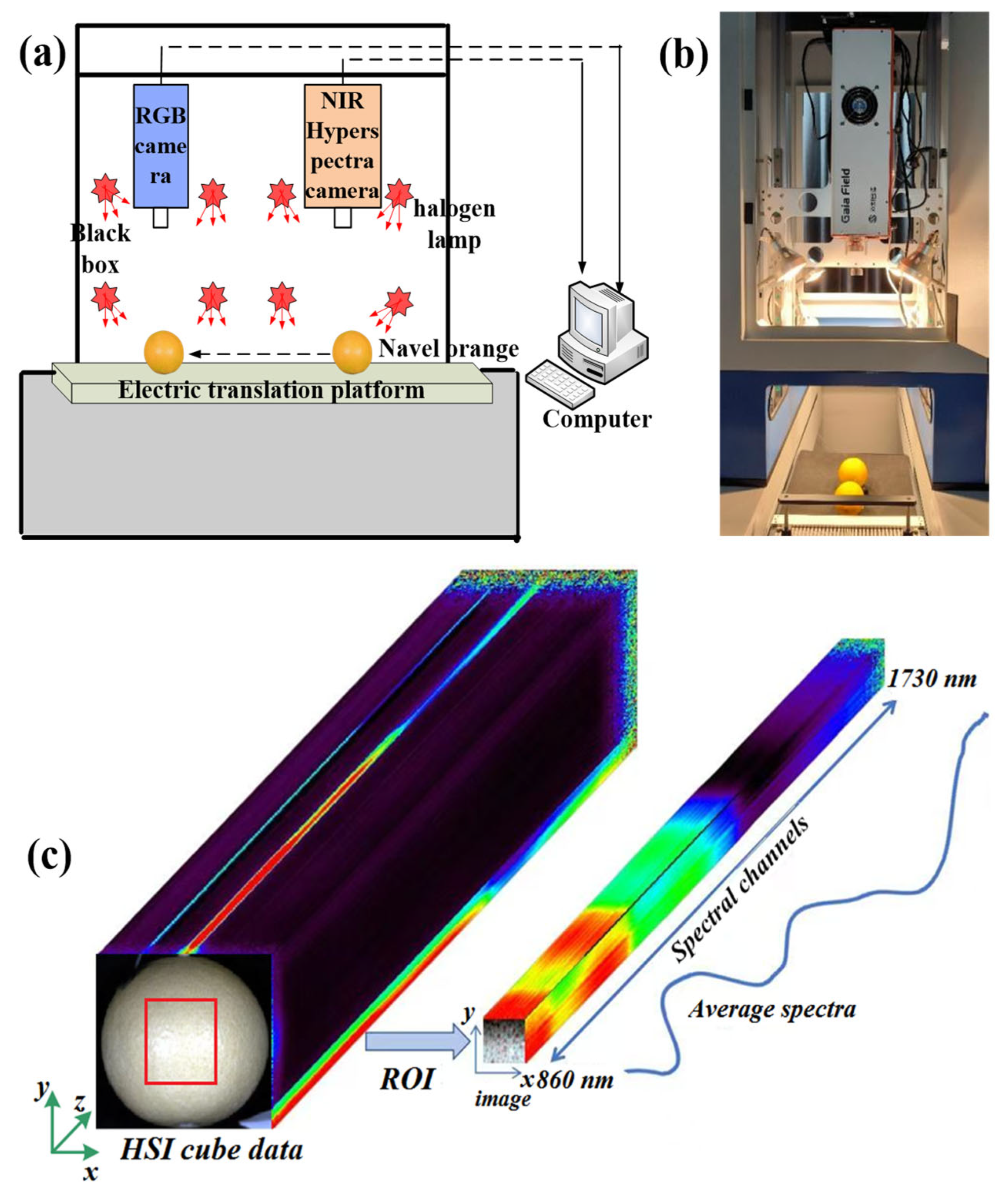
2.2. Devices
2.3. Hyperspectral Data Correction
2.4. ROI Extraction and Sample Partitioning
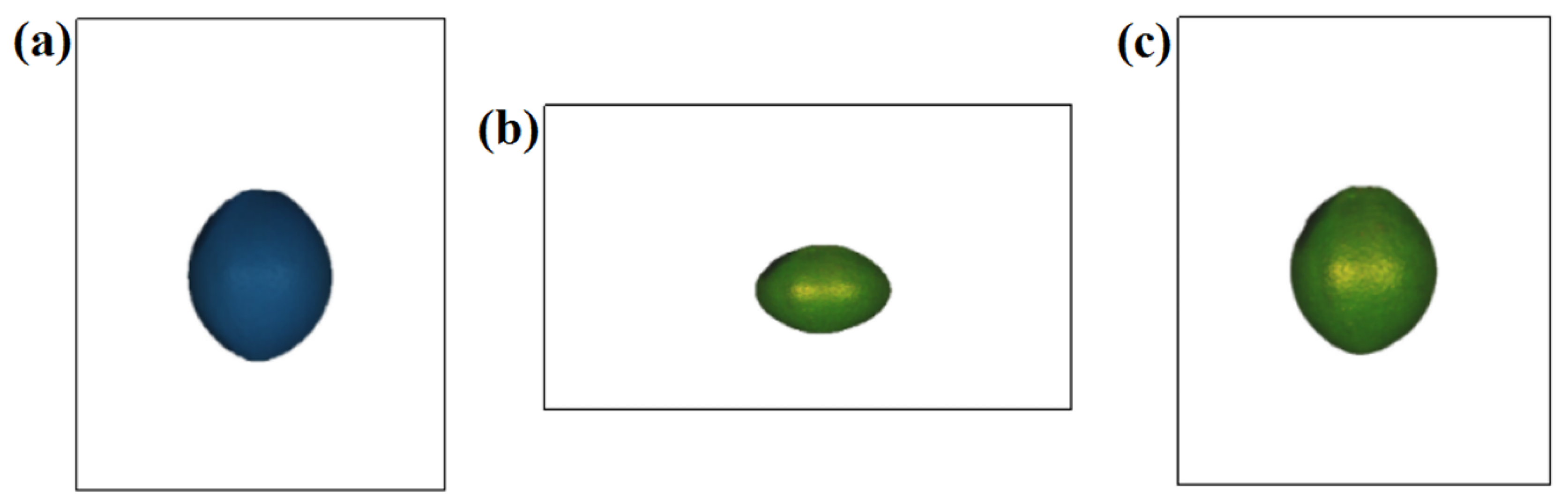
2.5. Image Registration
2.6. Data Processing
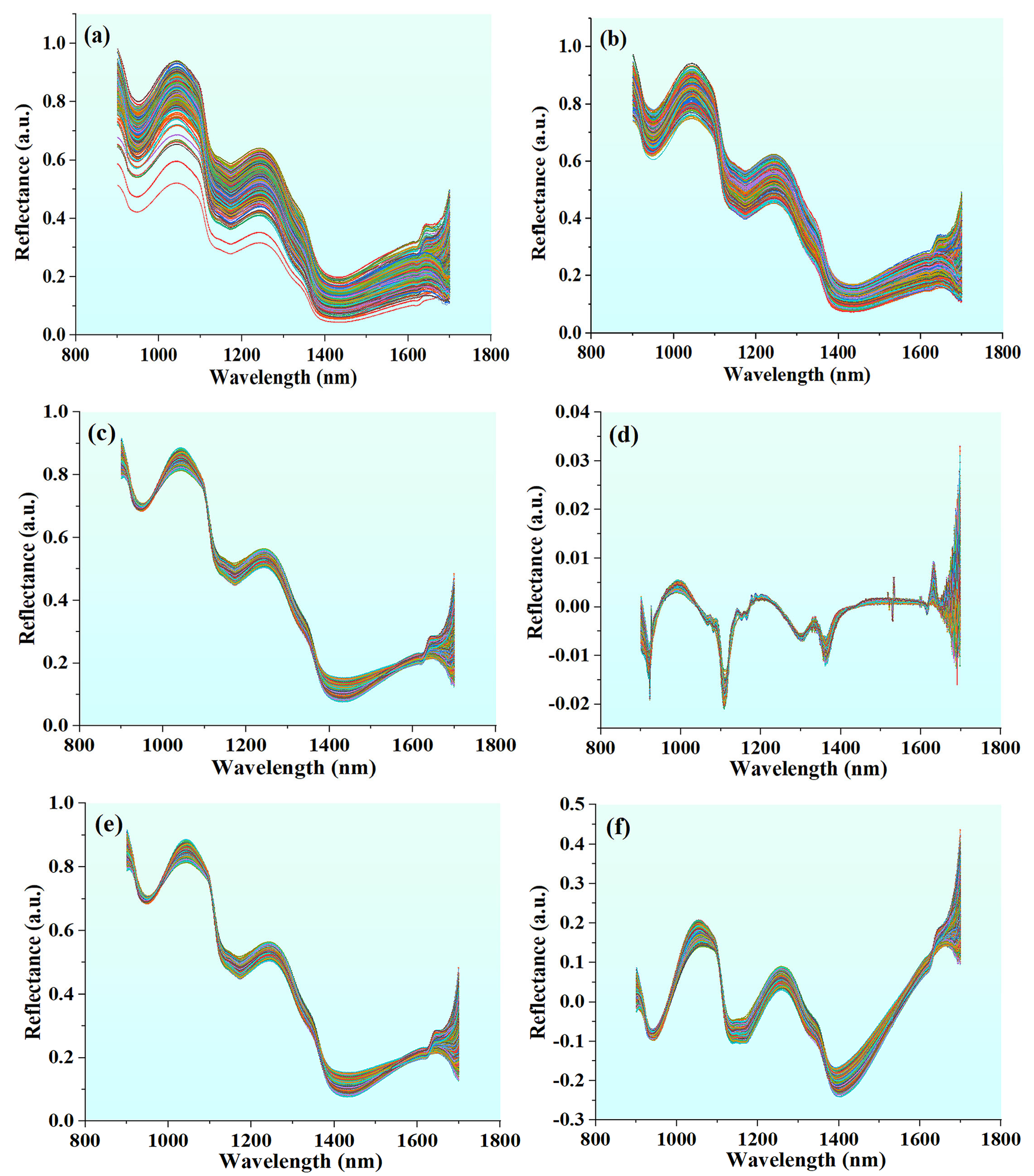
2.6.1. Spectral Preprocessing
2.6.2. Dimensionality Reduction of Hyperspectral Images
2.7. Discrimination Modeling
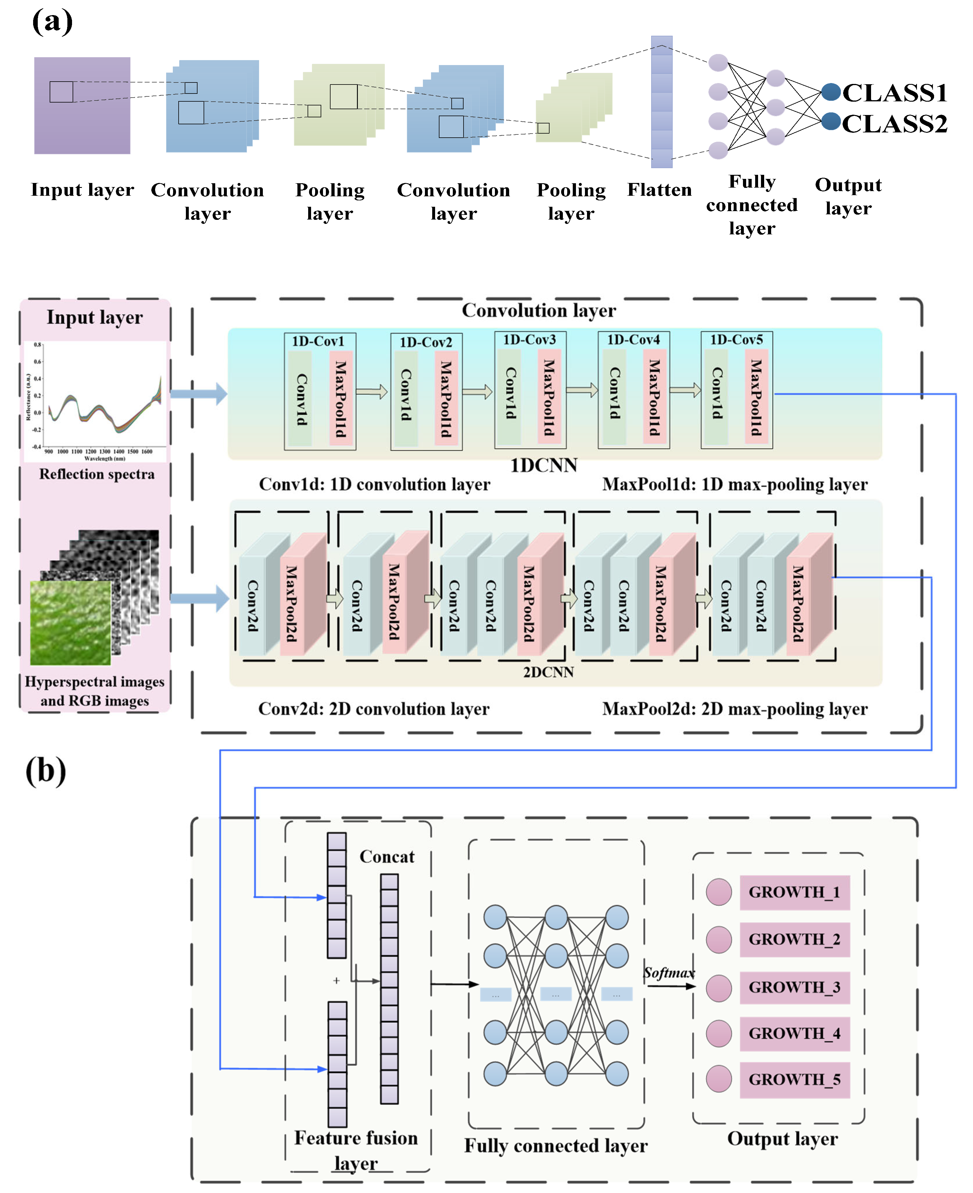
2.7.1. CNN
2.7.2. Proposed Novel Deep-Learning Model
2.7.3. Model Evaluation
3. Results and Analysis
3.1. Results of Abnormal Sample Elimination
3.2. Results of Spectral Preprocessing
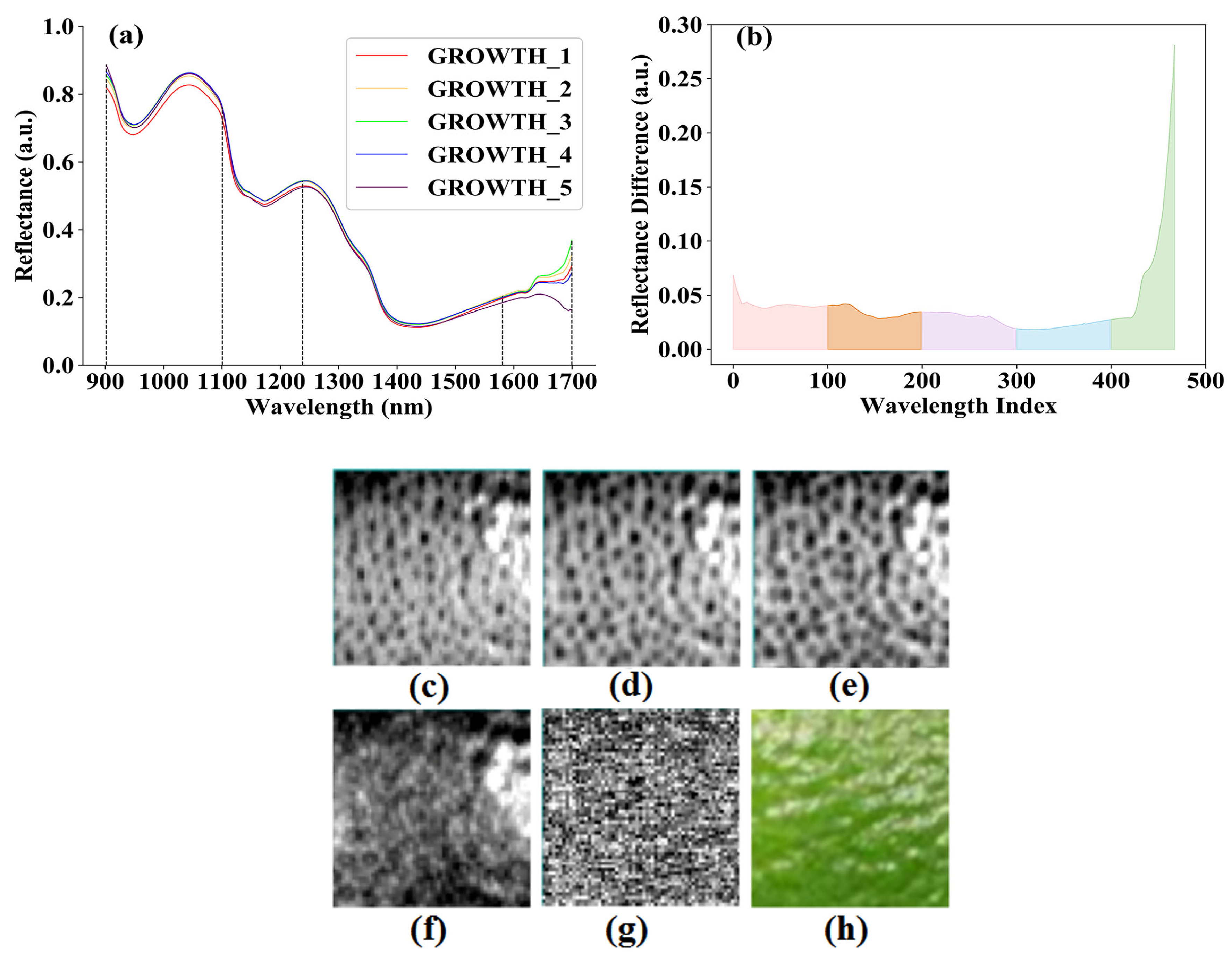
3.3. Results of Feature Wavelength Selection for Spectral Data
3.4. Results of Image Registration
3.5. Result of Optimal Selection of Feature Wavelengths for Hyperspectral Images
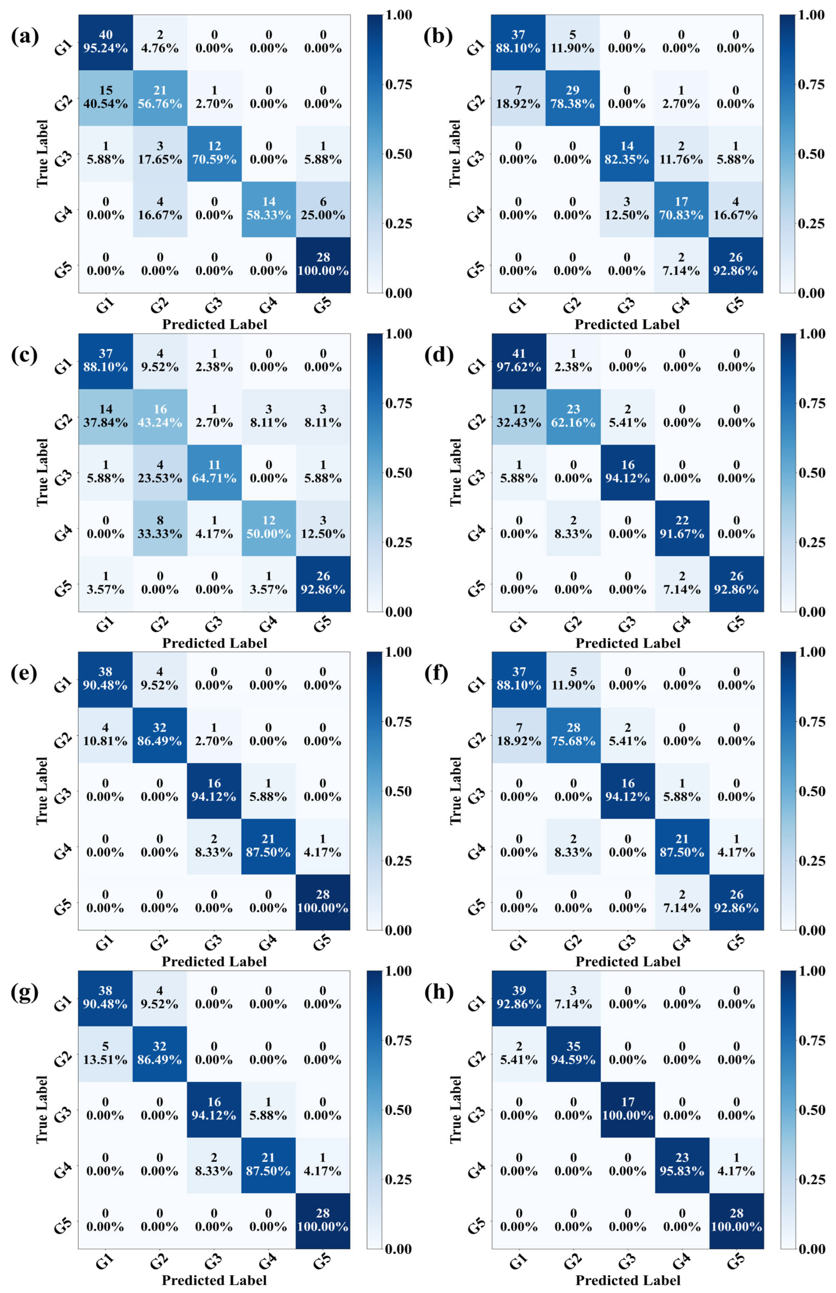
3.6. Results of Modeling Analysis
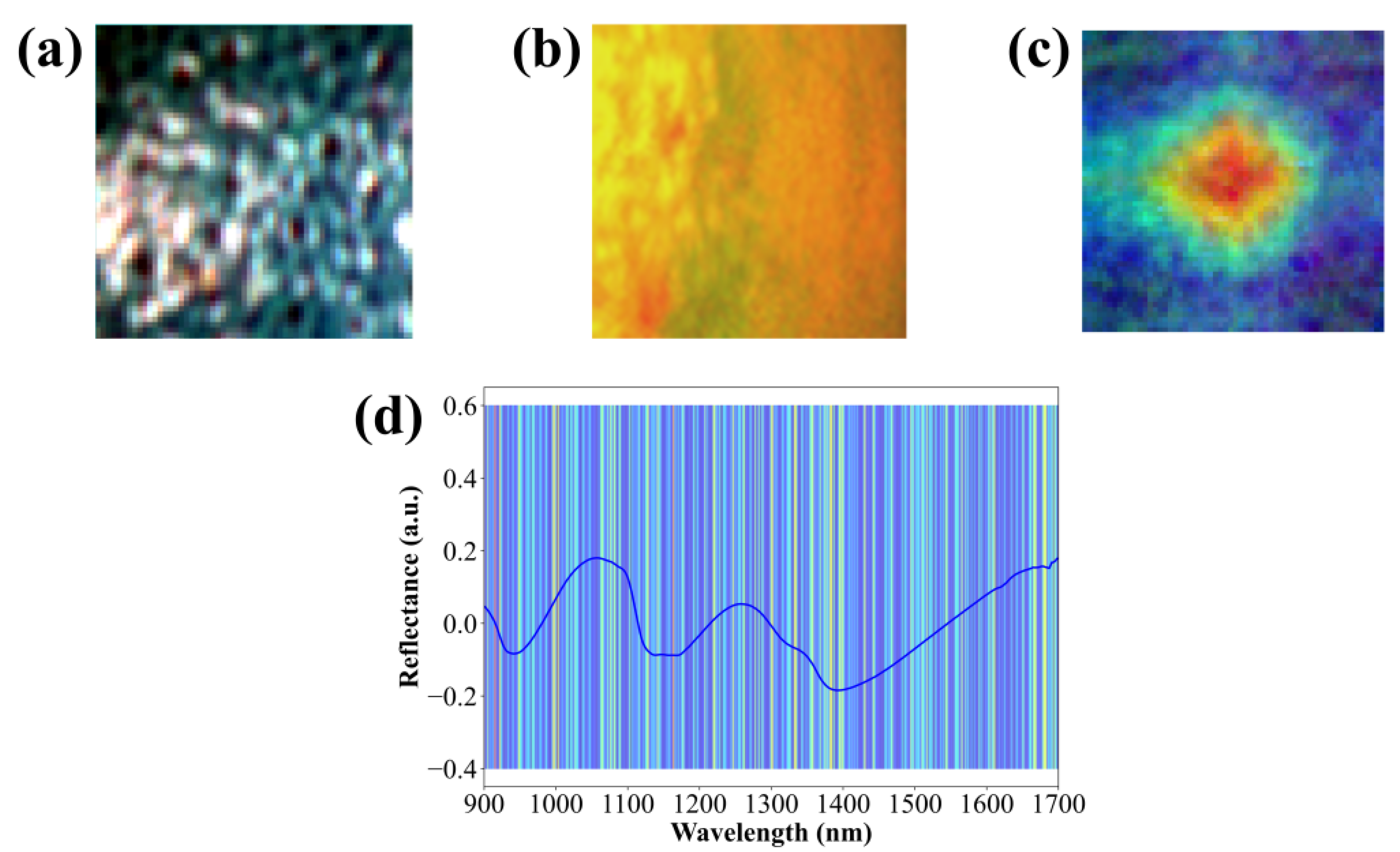
3.7. Interpretability Analysis of Growth Stage Discrimination Based on 1DCNN-VGG11 Model
4. Discussion
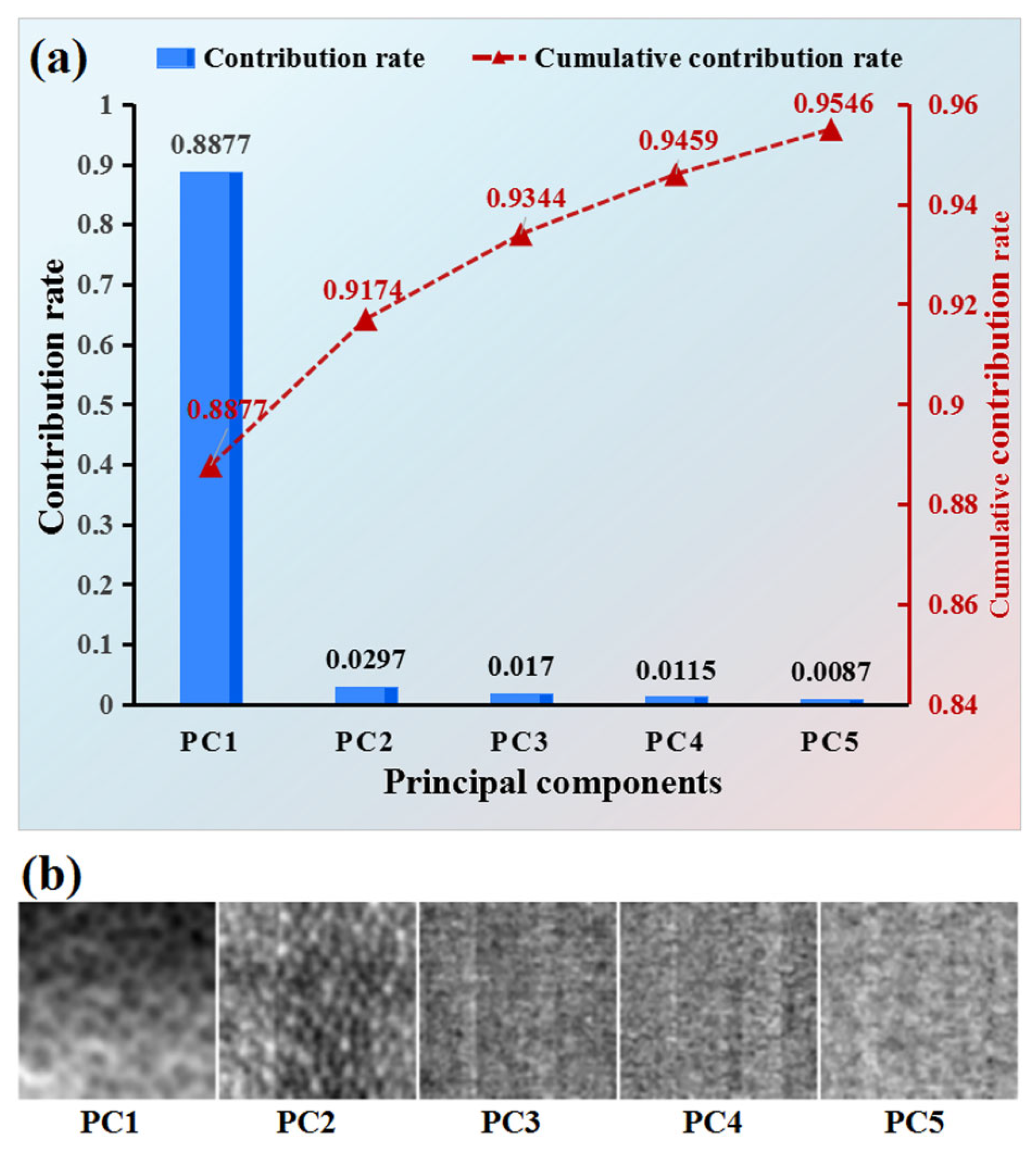
4.1. Comparison Between Hyperspectral Images Selected via Proposed Feature Selection and PCA
4.2. Comparison of Hyperspectral Images with Different Optimal Feature Wavelengths
4.3. Comparison with Previous Studies
5. Conclusions
Supplementary Materials
Author Contributions
Funding
Institutional Review Board Statement
Data Availability Statement
Conflicts of Interest
References
- Wan, C.; Kahramanoğlu, İ.; Chen, J.; Gan, Z.; Chen, C. Effects of Hot Air Treatments on Postharvest Storage of Newhall Navel Orange. Plants 2020, 9, 170. [Google Scholar] [CrossRef] [PubMed]
- Sun, Y.; Li, Y.; Xu, Y.; Sang, Y.; Mei, S.; Xu, C.; Yu, X.; Pan, T.; Cheng, C.; Zhang, J.; et al. The Effects of Storage Temperature, Light Illumination, and Low-Temperature Plasma on Fruit Rot and Change in Quality of Postharvest Gannan Navel Oranges. Foods 2022, 11, 3707. [Google Scholar] [CrossRef] [PubMed]
- Wang, F.; Zhao, C.; Yang, H.; Jiang, H.; Li, L.; Yang, G. Non-Destructive and in-Site Estimation of Apple Quality and Ma-turity by Hyperspectral Imaging. Comput. Electron. Agric. 2022, 195, 106843. [Google Scholar] [CrossRef]
- Khodabakhshian, R.; Emadi, B. Application of Vis/SNIR Hyperspectral Imaging in Ripeness Classification of Pear. Int. J. Food Prop. 2017, 20, S3149–S3163. [Google Scholar] [CrossRef]
- Beć, K.B.; Grabska, J.; Huck, C.W. Principles and Applications of Miniaturized Near-Infrared (NIR) Spectrometers. Chem.—A Eur. J. 2021, 27, 1514–1532. [Google Scholar] [CrossRef] [PubMed]
- Chu, X.; Miao, P.; Zhang, K.; Wei, H.; Fu, H.; Liu, H.; Jiang, H.; Ma, Z. Green Banana Maturity Classification and Quality Evaluation Using Hyperspectral Imaging. Agriculture 2022, 12, 530. [Google Scholar] [CrossRef]
- Ye, W.; Xu, W.; Yan, T.; Yan, J.; Gao, P.; Zhang, C. Application of Near-Infrared Spectroscopy and Hyperspectral Imaging Combined with Machine Learning Algorithms for Quality Inspection of Grape: A Review. Foods 2022, 12, 132. [Google Scholar] [CrossRef] [PubMed]
- Ozdemir, A.; Polat, K. Deep Learning Applications for Hyperspectral Imaging: A Systematic Review. J. Inst. Electron. Comput. 2020, 2, 39–56. [Google Scholar] [CrossRef]
- Benelli, A.; Cevoli, C.; Ragni, L.; Fabbri, A. In-Field and Non-Destructive Monitoring of Grapes Maturity by Hyperspectral Imaging. Biosyst. Eng. 2021, 207, 59–67. [Google Scholar] [CrossRef]
- Zhao, M.; Cang, H.; Chen, H.; Zhang, C.; Yan, T.; Zhang, Y.; Gao, P.; Xu, W. Determination of Quality and Maturity of Pro-cessing Tomatoes Using Near-Infrared Hyperspectral Imaging with Interpretable Machine Learning Methods. LWT 2023, 183, 114861. [Google Scholar] [CrossRef]
- Shao, Y.; Ji, S.; Shi, Y.; Xuan, G.; Jia, H.; Guan, X.; Chen, L. Growth Period Determination and Color Coordinates Visual Analysis of Tomato Using Hyperspectral Imaging Technology. Spectrochim. Acta A Mol. Biomol. Spectrosc. 2024, 319, 124538. [Google Scholar] [CrossRef] [PubMed]
- Shang, M.; Xue, L.; Zhang, Y.; Liu, M.; Li, J. Full-surface Defect Detection of Navel Orange Based on Hyperspectral Online Sorting Technology. J. Food Sci. 2023, 88, 2488–2495. [Google Scholar] [CrossRef] [PubMed]
- Ye, W.; Yan, T.; Zhang, C.; Duan, L.; Chen, W.; Song, H.; Zhang, Y.; Xu, W.; Gao, P. Detection of Pesticide Residue Level in Grape Using Hyperspectral Imaging with Machine Learning. Foods 2022, 11, 1609. [Google Scholar] [CrossRef] [PubMed]
- Wei, X.; He, J.-C.; Ye, D.-P.; Jie, D.-F. Navel Orange Maturity Classification by Multispectral Indexes Based on Hyperspec-tral Diffuse Transmittance Imaging. J. Food Qual. 2017, 2017, 1–7. [Google Scholar] [CrossRef]
- Luo, W.; Zhang, J.; Huang, H.; Peng, W.; Gao, Y.; Zhan, B.; Zhang, H. Prediction of Fat Content in Salmon Fillets Based on Hyperspectral Imaging and Residual Attention Convolution Neural Network. LWT 2023, 184, 115018. [Google Scholar] [CrossRef]
- Jia, S.; Jiang, S.; Lin, Z.; Li, N.; Xu, M.; Yu, S. A Survey: Deep Learning for Hyperspectral Image Classification with Few Labeled Samples. Neurocomputing 2021, 448, 179–204. [Google Scholar] [CrossRef]
- Varga, L.A.; Makowski, J.; Zell, A. Measuring the Ripeness of Fruit with Hyperspectral Imaging and Deep Learning. In Proceedings of the 2021 International Joint Conference on Neural Networks (IJCNN), Shenzhen, China, 18–22 July 2021; IEEE: New York, NY, USA, 2021; pp. 1–8. [Google Scholar]
- Benmouna, B.; García-Mateos, G.; Sabzi, S.; Fernandez-Beltran, R.; Parras-Burgos, D.; Molina-Martínez, J.M. Convolutional Neural Networks for Estimating the Ripening State of Fuji Apples Using Visible and Near-Infrared Spectroscopy. Food Bioproc. Tech. 2022, 15, 2226–2236. [Google Scholar] [CrossRef]
- Zhou, X.; Liu, W.; Li, K.; Lu, D.; Su, Y.; Ju, Y.; Fang, Y.; Yang, J. Discrimination of Maturity Stages of Cabernet Sauvignon Wine Grapes Using Visible–Near-Infrared Spectroscopy. Foods 2023, 12, 4371. [Google Scholar] [CrossRef] [PubMed]
- Han, Y.; Bai, S.H.; Trueman, S.J.; Khoshelham, K.; Kämper, W. Predicting the Ripening Time of ‘Hass’ and ‘Shepard’ Avo-cado Fruit by Hyperspectral Imaging. Precis. Agric. 2023, 24, 1889–1905. [Google Scholar] [CrossRef]
- Tao, Z.; Li, K.; Rao, Y.; Li, W.; Zhu, J. Strawberry Maturity Recognition Based on Improved YOLOv5. Agronomy 2024, 14, 460. [Google Scholar] [CrossRef]
- Su, Z.; Zhang, C.; Yan, T.; Zhu, J.; Zeng, Y.; Lu, X.; Gao, P.; Feng, L.; He, L.; Fan, L. Application of Hyperspectral Imaging for Maturity and Soluble Solids Content Determination of Strawberry With Deep Learning Approaches. Front. Plant Sci. 2021, 12, 736334. [Google Scholar] [CrossRef] [PubMed]
- Zhang, L.; Guan, Y.; Wang, N.; Ge, F.; Zhang, Y.; Zhao, Y. Identification of Growth Years for Puerariae Thomsonii Radix Based on Hyperspectral Imaging Technology and Deep Learning Algorithm. Sci. Rep. 2023, 13, 14286. [Google Scholar] [CrossRef] [PubMed]
- Han, L.; Tian, J.; Huang, Y.; He, K.; Liang, Y.; Hu, X.; Xie, L.; Yang, H.; Huang, D. Hyperspectral Imaging Combined with Dual-Channel Deep Learning Feature Fusion Model for Fast and Non-Destructive Recognition of Brew Wheat Varieties. J. Food Compos. Anal. 2024, 125, 105785. [Google Scholar] [CrossRef]
- An, D.; Zhang, L.; Liu, Z.; Liu, J.; Wei, Y. Advances in Infrared Spectroscopy and Hyperspectral Imaging Combined with Artificial Intelligence for the Detection of Cereals Quality. Crit. Rev. Food Sci. Nutr. 2023, 63, 9766–9796. [Google Scholar] [CrossRef] [PubMed]
- Garillos-Manliguez, C.A.; Chiang, J.Y. Multimodal Deep Learning and Visible-Light and Hyperspectral Imaging for Fruit Maturity Estimation. Sensors 2021, 21, 1288. [Google Scholar] [CrossRef] [PubMed]
- Whitfield, R.G.; Gerger, M.E.; Sharp, R.L. Near-Infrared Spectrum Qualification via Mahalanobis Distance Determination. Appl. Spectrosc. 1987, 41, 1204–1213. [Google Scholar] [CrossRef]
- Wang, Z.; Bovik, A.C.; Sheikh, H.R.; Simoncelli, E.P. Image Quality Assessment: From Error Visibility to Structural Similarity. IEEE Trans. Image Process. 2004, 13, 600–612. [Google Scholar] [CrossRef] [PubMed]
- Rinnan, Å.; Berg, F.v.d.; Engelsen, S.B. Review of the Most Common Pre-Processing Techniques for near-Infrared Spectra. TrAC Trends Anal. Chem. 2009, 28, 1201–1222. [Google Scholar] [CrossRef]
- Dhanoa, M.S.; Lister, S.J.; Sanderson, R.; Barnes, R.J. The Link between Multiplicative Scatter Correction (MSC) and Stand-ard Normal Variate (SNV) Transformations of NIR Spectra. J. Near Infrared Spectrosc. 1994, 2, 43–47. [Google Scholar] [CrossRef]
- Savitzky, A.; Golay, M.J.E. Smoothing and Differentiation of Data by Simplified Least Squares Procedures. Anal. Chem. 1964, 36, 1627–1639. [Google Scholar] [CrossRef]
- Barnes, R.J.; Dhanoa, M.S.; Lister, S.J. Standard Normal Variate Transformation and De-Trending of Near-Infrared Diffuse Reflectance Spectra. Appl. Spectrosc. 1989, 43, 772–777. [Google Scholar] [CrossRef]
- Rodarmel, C.; Shan, J. Principal Component Analysis for Hyperspectral Image Classification; Semantic Scholar: Seattle, WA, USA, 2002; Volume 62. [Google Scholar]
- Li, Z.; Liu, F.; Yang, W.; Peng, S.; Zhou, J. A Survey of Convolutional Neural Networks: Analysis, Applications, and Prospects. IEEE Trans. Neural Netw. Learn. Syst. 2022, 33, 6999–7019. [Google Scholar] [CrossRef] [PubMed]
- Lasalvia, M.; Capozzi, V.; Perna, G. A Comparison of PCA-LDA and PLS-DA Techniques for Classification of Vibrational Spectra. Appl. Sci. 2022, 12, 5345. [Google Scholar] [CrossRef]
- Zhang, S.; Li, X.; Zong, M.; Zhu, X.; Wang, R. Efficient KNN Classification With Different Numbers of Nearest Neighbors. IEEE Trans. Neural Netw. Learn. Syst. 2018, 29, 1774–1785. [Google Scholar] [CrossRef] [PubMed]
- Jiang, T.; Zuo, W.; Ding, J.; Yuan, S.; Qian, H.; Cheng, Y.; Guo, Y.; Yu, H.; Yao, W. Machine Learning Driven Benchtop Vis/NIR Spectroscopy for Online Detection of Hybrid Citrus Quality. Food Res. Int. 2025, 201, 115617. [Google Scholar] [CrossRef] [PubMed]
- de Santana, F.B.; Borges Neto, W.; Poppi, R.J. Random Forest as One-Class Classifier and Infrared Spectroscopy for Food Adulteration Detection. Food Chem. 2019, 293, 323–332. [Google Scholar] [CrossRef] [PubMed]
- Hecht-Nielsen, R. Theory of the Backpropagation Neural Network. In Proceedings of the International Joint Conference on Neural Networks, Washington, DC, USA, 18–22 June 1989; Elsevier: Amsterdam, The Netherlands, 1992; pp. 65–93. [Google Scholar]
- Ahmed, S.; Hasan, M.B.; Ahmed, T.; Sony, M.R.K.; Kabir, M.H. Less Is More: Lighter and Faster Deep Neural Architec-ture for Tomato Leaf Disease Classification. IEEE Access 2022, 10, 68868–68884. [Google Scholar] [CrossRef]
- McHugh, M.L. Interrater Reliability: The Kappa Statistic. Biochem. Med. 2012, 22, 276–282. [Google Scholar] [CrossRef]
- Li, H.; Liang, Y.; Xu, Q.; Cao, D. Key Wavelengths Screening Using Competitive Adaptive Reweighted Sampling Method for Multivariate Calibration. Anal. Chim. Acta 2009, 648, 77–84. [Google Scholar] [CrossRef] [PubMed]
- Efron, B.; Hastie, T.; Johnstone, I.; Tibshirani, R. Least Angle Regression. Ann. Stat. 2004, 32, 407–499. [Google Scholar] [CrossRef]
- Centner, V.; Massart, D.-L.; de Noord, O.E.; de Jong, S.; Vandeginste, B.M.; Sterna, C. Elimination of Uninformative Varia-bles for Multivariate Calibration. Anal. Chem. 1996, 68, 3851–3858. [Google Scholar] [CrossRef] [PubMed]
- Fan, F.; Changwei, Z.; Xiaojun, Z.; Di, W.; Zhi, T.; Yishen, X. Feature Wavelength Selection in Near-Infrared Spectroscopy Based on Genetic Algorithm. In Proceedings of the 2021 International Conference on Sensing, Measurement & Data Analytics in the Era of Artificial Intelligence (ICSMD), Nanjing, China, 21–23 October 2021; IEEE: New York, NY, USA, 2021; pp. 1–5. [Google Scholar]
- Li, L.; Doroslovacki, M.; Loew, M.H. Approximating the Gradient of Cross-Entropy Loss Function. IEEE Access 2020, 8, 111626–111635. [Google Scholar] [CrossRef]
- Salehin, I.; Kang, D.-K. A Review on Dropout Regularization Approaches for Deep Neural Networks within the Scholarly Domain. Electronics 2023, 12, 3106. [Google Scholar] [CrossRef]
- Frazier, P.I. Bayesian Optimization. In Recent Advances in Optimization and Modeling of Contemporary Problems; INFORMS: Catonsville, MD, USA, 2018; pp. 255–278. [Google Scholar]
- Al-Kababji, A.; Bensaali, F.; Dakua, S.P. Scheduling Techniques for Liver Segmentation: ReduceLRonPlateau vs. OneCy-cleLR; Springer: Berlin/Heidelberg, Germany, 2022; pp. 204–212. [Google Scholar]
- Selvaraju, R.R.; Cogswell, M.; Das, A.; Vedantam, R.; Parikh, D.; Batra, D. Grad-CAM: Visual Explanations from Deep Net-works via Gradient-Based Localization. Int. J. Comput. Vis. 2020, 128, 336–359. [Google Scholar] [CrossRef]
- Liu, J.; Meng, H. Research on the Maturity Detection Method of Korla Pears Based on Hyperspectral Technology. Agriculture 2024, 14, 1257. [Google Scholar] [CrossRef]
- Qiu, G.; Lu, H.; Wang, X.; Wang, C.; Xu, S.; Liang, X.; Fan, C. Nondestructive Detecting Maturity of Pineapples Based on Visible and Near-Infrared Transmittance Spectroscopy Coupled with Machine Learning Methodologies. Horticulturae 2023, 9, 889. [Google Scholar] [CrossRef]
- Zheng, L.; Zhao, M.; Zhu, J.; Huang, L.; Zhao, J.; Liang, D.; Zhang, D. Fusion of Hyperspectral Imaging (HSI) and RGB for Identification of Soybean Kernel Damages Using ShuffleNet with Convolutional Optimization and Cross Stage Partial Architec-ture. Front. Plant Sci. 2023, 13, 1098864. [Google Scholar] [CrossRef] [PubMed]
- Zhang, H.; Jiang, X.; Liu, L.; Wang, H.; Wang, Y. S2F2AN: Spatial–Spectral Fusion Frequency Attention Network for Chi-nese Herbal Medicines Hyperspectral Image Segmentation. IEEE Trans. Instrum. Meas. 2025, 74, 1–13. [Google Scholar] [CrossRef]


| Cultivar | Growth_1 | Growth_2 | Growth_3 | Growth_4 | Growth_5 | Numbers |
|---|---|---|---|---|---|---|
| Newhall |  23 August– 5 October |  6 October– 7 November |  8 November– 18 November |  19 November– 29 November |  30 November– 10 December | 159 |
| Navelina |  23 August– 16 October |  17 October– 27 October |  28 October– 8 November |  9 November– 19 November |  20 November– 10 December | 159 |
| CaraCara |  23 August– 16 October |  17 October– 7 November |  8 November– 18 November |  19 November– 29 November |  30 November– 10 December | 159 |
| Gannan No.1 |  23 August– 13 September |  14 September– 16 October |  17 October– 27 October |  28 October– 19 November |  20 November– 10 December | 159 |
| Gannan No.5 |  23 August– 13 September |  14 September– 16 October |  17 October– 27 October |  28 October– 19 November |  20 November– 10 December | 159 |
| Growth Period | Raw Samples | Before Removal for Valid Samples | After Removal for Valid Samples | ||
|---|---|---|---|---|---|
| Training Set | Testing Set | Total Number | |||
| Growth_1 | 270 | 255 | 205 | 42 | 247 |
| Growth_2 | 180 | 178 | 131 | 37 | 168 |
| Growth_3 | 81 | 79 | 57 | 17 | 74 |
| Growth_4 | 120 | 119 | 91 | 24 | 115 |
| Growth_5 | 144 | 144 | 108 | 28 | 136 |
| Total number | 795 | 775 | 592 | 148 | 740 |
| Preprocessing Method | PCs 1 | Training Set | Testing Set | 10-Fold CV | |||
|---|---|---|---|---|---|---|---|
| AC (%) | AC (%) | RC (%) | PC (%) | F1 (%) | AC (%) | ||
| RAW | 20 | 81.59 | 79.73 | 73.47 | 83.83 | 73.26 | 76.04 |
| FD | 19 | 91.55 | 78.38 | 77.06 | 78.66 | 77.58 | 79.06 |
| DT | 18 | 79.05 | 77.03 | 72.36 | 81.8 | 72.47 | 75.53 |
| MSC | 19 | 79.9 | 77.7 | 72.77 | 82.73 | 72.83 | 75.68 |
| SG | 19 | 79.39 | 77.7 | 72.2 | 82.75 | 71.94 | 75.53 |
| FD + DT | 20 | 90.2 | 79.73 | 77.59 | 80.93 | 78.41 | 78.21 |
| FD + SG | 19 | 82.94 | 78.38 | 73.79 | 82.85 | 74.45 | 76.69 |
| DT + SG | 16 | 77.87 | 75 | 70.51 | 80.68 | 70.9 | 75.19 |
| MSC + FD | 14 | 86.99 | 79.05 | 76.64 | 80.87 | 77.89 | 76.01 |
| MSC + SG | 17 | 78.55 | 78.38 | 73.67 | 82.81 | 73.66 | 74.68 |
| MSC + DT | 20 | 82.43 | 80.41 | 75.34 | 83.9 | 75.86 | 78.05 |
| Feature Wavelength Selection Method | PCs | Training Set | Testing Set | 10-Fold CV | |||
|---|---|---|---|---|---|---|---|
| AC (%) | AC (%) | RC (%) | PC (%) | F1 (%) | AC (%) | ||
| None | 20 | 82.43 | 80.41 | 75.34 | 83.90 | 75.86 | 78.05 |
| CARS | 16 | 77.53 | 75.68 | 70.70 | 80.18 | 70.69 | 74.34 |
| LAR | 18 | 80.41 | 76.35 | 71.06 | 81.42 | 70.30 | 75.68 |
| UVE | 19 | 78.89 | 79.73 | 73.76 | 84.43 | 73.54 | 76.53 |
| GA | 17 | 79.90 | 79.05 | 73.51 | 83.81 | 72.80 | 76.71 |
| Data Modal | Model | Training Set | Testing Set | ||||
|---|---|---|---|---|---|---|---|
| AC (%) | AC (%) | RC (%) | PC (%) | F1 (%) | Kappa | ||
| Spectra | PLS-DA | 82.43 | 80.41 | 75.34 | 83.9 | 75.86 | 0.7459 |
| SVM | 97.97 | 87.16 | 88.49 | 89.27 | 88.82 | 0.8356 | |
| RF | 99.16 | 76.35 | 76.64 | 77.47 | 76.37 | 0.6963 | |
| KNN | 100 | 70.27 | 68.29 | 69.03 | 68.09 | 0.6175 | |
| BPNN | 77.42 | 76.35 | 79.72 | 78.9 | 78.31 | 0.6995 | |
| 1DCNN | 83.33 | 77.7 | 76.18 | 82.75 | 77.38 | 0.7111 | |
| Hyperspectral images | ResNet18 | 99.33 | 68.24 | 64.91 | 75.96 | 66.49 | 0.5849 |
| AlexNet | 77.37 | 60.81 | 61.09 | 61.25 | 60.45 | 0.4953 | |
| VGG11 | 100 | 68.92 | 67.78 | 70.43 | 68.1 | 0.5983 | |
| RGB images | ResNet18 | 97.54 | 83.78 | 83.97 | 85.82 | 84.35 | 0.7916 |
| AlexNet | 85.27 | 87.16 | 87.83 | 88.44 | 87.99 | 0.8355 | |
| VGG11 | 86.85 | 83.11 | 82.5 | 82.58 | 82.43 | 0.7838 | |
| Hyperspectral images + RGB images | ResNet18 | 99.03 | 91.22 | 91.78 | 91.6 | 91.63 | 0.8877 |
| AlexNet | 89.08 | 89.86 | 89.72 | 90.77 | 90.17 | 0.8701 | |
| VGG11 | 91.88 | 91.22 | 91.72 | 91.12 | 91.32 | 0.8878 | |
| Spectra + Hyperspectral images | 1DCNN-ResNet18 | 100 | 85.14 | 85.86 | 86.59 | 85.9 | 0.8095 |
| 1DCNN-AlexNet | 99.83 | 87.84 | 88.89 | 90.25 | 89.38 | 0.8438 | |
| 1DCNN-VGG11 | 100 | 86.49 | 87.68 | 88.99 | 87.56 | 0.8265 | |
| Spectra + Hyperspectral images + RGB images | LSTM-LSTM | 84.81 | 86.49 | 87.53 | 88.21 | 87.54 | 0.8269 |
| LSTM-VGG11 | 95.96 | 91.22 | 91.72 | 91.63 | 91.61 | 0.8876 | |
| LSTM-ResNet18 | 97.24 | 90.54 | 91.47 | 91.8 | 91.57 | 0.8789 | |
| LSTM-AlexNet | 92.6 | 86.49 | 86.04 | 89.09 | 86.97 | 0.8263 | |
| 1DCNN-LSTM | 100 | 86.49 | 87.65 | 87.36 | 87.46 | 0.8271 | |
| 1DCNN-ResNet18 | 100 | 91.22 | 91.76 | 92.12 | 91.72 | 0.8875 | |
| 1DCNN-AlexNet | 99.84 | 91.22 | 92.18 | 91.48 | 91.73 | 0.8878 | |
| 1DCNN-VGG11 | 100 | 95.95 | 96.66 | 96.76 | 96.69 | 0.9481 | |
| Data Features | Model | Training Set | Testing Set | ||||
|---|---|---|---|---|---|---|---|
| AC (%) | AC (%) | RC (%) | PC (%) | F1 (%) | Kappa | ||
| Spectra + RGB images + Hyperspectral images with proposed method | 1DCNN-VGG11 | 100 | 95.95 | 96.66 | 96.76 | 96.69 | 0.9481 |
| Spectra + RGB images + Hyperspectral images with PCA | 1DCNN-VGG11 | 100 | 93.92 | 94.93 | 94.88 | 94.9 | 0.9222 |
| Data Features | Model | Training Set | Testing Set | ||||
|---|---|---|---|---|---|---|---|
| AC (%) | AC (%) | RC (%) | PC (%) | F1 (%) | Kappa | ||
| Spectra + RGB images + Hyperspectral images with 3 bands | 1DCNN-VGG11 | 100 | 93.92 | 94.81 | 94.63 | 94.65 | 0.9222 |
| Spectra + RGB images + Hyperspectral images with 5 bands | 1DCNN-VGG11 | 100 | 95.95 | 96.66 | 96.76 | 96.69 | 0.9481 |
| Spectra + RGB images + Hyperspectral images with 7 bands | 1DCNN-VGG11 | 100 | 95.27 | 96.25 | 96.35 | 96.19 | 0.9395 |
| Spectra + RGB images + Hyperspectral images with 9 bands | 1DCNN-VGG11 | 100 | 94.59 | 95.35 | 95.15 | 95.17 | 0.9309 |
| Fruit | Number of Cultivars | Objective | Method | Model | AC (%) | Ref. |
|---|---|---|---|---|---|---|
| Grape | one | Maturity | HSI | PLS-DA | 91 | [9] |
| Tomato | one | Growth stage | HSI | Linear DA (LDA) | 93.1 | [11] |
| Avocado/Kiwi | one | Ripeness | HSI | CNN | 93.3/66.7 | [17] |
| Grape | one | Maturity | Vis-NIR spectroscopy | Stacked autoencoders (SAE) | 94 | [19] |
| Strawberry | one | Maturity | HSI | 1D ResNet | 86.03 | [22] |
| Papaya | one | Maturity | Vis imaging and HSI | Multi-modal VGG16 | 88.64 | [26] |
| Korla Pear | one | Maturity | HSI | BPNN | 93.5 | [51] |
| Pineapple | one | Maturity | Vis/NIR transmittance spectroscopy | PLS-DA | 90.8 | [52] |
| Navel orange | five | Growth stage | NIR spectroscopy, HSI, and RGB imaging | Multi-modal dual-branch model (1DCNN-VGG11) | 95.95 | ours |
Disclaimer/Publisher’s Note: The statements, opinions and data contained in all publications are solely those of the individual author(s) and contributor(s) and not of MDPI and/or the editor(s). MDPI and/or the editor(s) disclaim responsibility for any injury to people or property resulting from any ideas, methods, instructions or products referred to in the content. |
© 2025 by the authors. Licensee MDPI, Basel, Switzerland. This article is an open access article distributed under the terms and conditions of the Creative Commons Attribution (CC BY) license (https://creativecommons.org/licenses/by/4.0/).
Share and Cite
Zhao, C.; Ren, Z.; Li, Y.; Zhang, J.; Shi, W. Growth Stages Discrimination of Multi-Cultivar Navel Oranges Using the Fusion of Near-Infrared Hyperspectral Imaging and Machine Vision with Deep Learning. Agriculture 2025, 15, 1530. https://doi.org/10.3390/agriculture15141530
Zhao C, Ren Z, Li Y, Zhang J, Shi W. Growth Stages Discrimination of Multi-Cultivar Navel Oranges Using the Fusion of Near-Infrared Hyperspectral Imaging and Machine Vision with Deep Learning. Agriculture. 2025; 15(14):1530. https://doi.org/10.3390/agriculture15141530
Chicago/Turabian StyleZhao, Chunyan, Zhong Ren, Yue Li, Jia Zhang, and Weinan Shi. 2025. "Growth Stages Discrimination of Multi-Cultivar Navel Oranges Using the Fusion of Near-Infrared Hyperspectral Imaging and Machine Vision with Deep Learning" Agriculture 15, no. 14: 1530. https://doi.org/10.3390/agriculture15141530
APA StyleZhao, C., Ren, Z., Li, Y., Zhang, J., & Shi, W. (2025). Growth Stages Discrimination of Multi-Cultivar Navel Oranges Using the Fusion of Near-Infrared Hyperspectral Imaging and Machine Vision with Deep Learning. Agriculture, 15(14), 1530. https://doi.org/10.3390/agriculture15141530