Coverage Path Planning Based on Region Segmentation and Path Orientation Optimization

Abstract

To address the operational demands of irregular farmland with fixed obstacles, this study proposes a full-coverage path planning framework that integrates UAV-based 3D perception and angle-adaptive optimization. First, digital orthophoto maps (DOMs) and digital elevation models (DEMs) were reconstructed from low-altitude aerial imagery. The feasible working region was constructed by shrinking field boundaries inward and dilating obstacle boundaries outward. This ensured sufficient safety margins for machinery operation. Next, segmentation angles were scanned from 0° to 180° to minimize the number and irregularity of sub-regions; then a two-level simulation search was performed over 0° to 360° to optimize the working direction for each sub-region. For each sub-region, the optimal working direction was selected based on four criteria: the number of turns, travel distance, coverage redundancy, and planning time. Between sub-regions, a closed-loop interconnection path was generated using eight-directional A* search combined with polyline simplification, arc fitting, Chaikin subdivision, and B-spline smoothing. Simulation results showed that a 78° segmentation yielded four regular sub-regions, achieving 99.97% coverage while reducing the number of turns, travel distance, and planning time by up to 70.42%, 23.17%, and 85.6%. This framework accounts for field heterogeneity and turning radius constraints, effectively mitigating path redundancy in conventional fixed-angle methods. This framework enables general deployment in agricultural field operations and facilitates extensions toward collaborative and energy-optimized task planning.

1. Introduction

With the continuous advancement of precision agriculture, intelligent agricultural machinery has been increasingly deployed in field operations. However, the complex field shapes, scattered obstacles, and terrain variability impose higher requirements on the adaptability and intelligence of path planning techniques [1,2,3]. Beyond ensuring complete area coverage, key challenges now include minimizing redundant travel and path overlap while optimizing path structure to enhance the automation level of agricultural operations [4,5].

Path planning approaches are generally classified into point-to-point path planning and complete coverage path planning (CCPP) [6,7,8]. The former focuses on optimizing routes between specific start and end points and is widely used in urban traffic and autonomous driving scenarios, with typical algorithms including A*, Artificial Potential Field (APF), and Rapidly-exploring Random Tree (RRT). While effective for obstacle avoidance and path length minimization, such methods are not suited to coverage-oriented agricultural tasks [9]. In contrast, CCPP better meets the needs of agricultural operations, emphasizing full area coverage while reducing turning frequency and redundant travel. Mainstream CCPP methods include evolutionary algorithm optimization, neural network-based path generation, and boustrophedon-based partitioning [10,11,12]. Among them, boustrophedon methods are widely adopted due to their simplicity and ease of implementation. These techniques decompose complex fields into regular sub-regions to simplify path generation [13,14,15]. However, most existing studies adopt fixed segmentation angles, often neglecting the impact of angle selection on planning effectiveness—leading to excessive path overlap and increased turning maneuvers in practice [16,17]. An unmanned aerial vehicle (UAV) is a remotely or autonomously operated aircraft platform capable of rapidly generating centimeter-level 3-D field maps from onboard RGB or LiDAR sensors. In practice, Zoto et al. used UAV orthomosaics to extract vine rows for UGV spraying [18]. Zhang et al. (2023) used five-band multispectral images captured by a UAV to map cotton verticillium-wilt severity with a random-forest model; the resulting prescription map guided a DJI T30 drone for variable-rate fungicide spraying [19].

In recent years, various optimization strategies have been proposed. For instance, Liu et al. developed a random-walk-based coverage strategy [20], which is easy to implement but lacks global efficiency. Schirmer et al. proposed a belief-space-based CCPP method that can ensure complete coverage under localization uncertainty [21]. Lu et al. introduced a bidirectional spiral path planning strategy to improve path smoothness and multi-robot task allocation [22]. While these methods perform well under specific conditions, they remain limited in fields with irregular shapes or dense obstacles [23]. Kharel et al. observed that even with GNSS-assisted guidance, the path redundancy rate in irregular fields ranged from 6% to 11%, leading to over-fertilization, chemical overdosing, and increased soil compaction [24]. On the software side, Mier et al. developed the Fields2Cover framework based on the ROS platform, focusing on path generation in regular fields. In simulations on the Nilsson benchmark field, the turning distance accounted for 0.5–50% of total path length [25]. In efforts to improve path coherence, Yang et al. applied an improved ant colony optimization (IACO) algorithm to tillage operations, reducing the objective function value by 47% compared with traditional ACO. However, the resulting paths still contained excessive zigzag segments, failing to fundamentally reduce non-operational distances [26]. Regarding UAV-based mapping, some studies rely solely on 2D orthomosaics: Mansur et al. convert UAV orthomosaics into crop-row centerlines to guide simple back-and-forth traversal, relying on naïve U-turns between rows [27]. By contrast, commercial tools such as DJI Terra can produce centimeter-level 3D point-cloud maps, offering richer spatial detail for more advanced path planning. In the Chinese context, Gao Chunlin used set covering and minimum Steiner tree principles for field connectivity optimization [28], while Liu Hui enhanced robustness in complex terrain path planning using an improved Whale Optimization Algorithm [29]. Wang Meng applied an ant colony algorithm for multi-machine cooperative scheduling [1], and Yang Lili achieved effective path smoothing using quadratic programming techniques [30].

Given the limitations in current research regarding path flexibility, segmentation angle diversity, and spatial modeling accuracy, this paper proposes a more practical CCPP framework integrating UAV photogrammetry-based 3D reconstruction and angular optimization. First, UAV photogrammetry is used to generate high-resolution digital orthophoto maps (DOMs) and digital elevation models (DEMs), from which precise field contours and obstacle locations are extracted via geometric preprocessing. Taking into account the machine turning radius and working width, a polygonal buffer-based shrinkage technique is applied to shrink field boundaries and expand obstacle margins to ensure safety and feasibility; this process is implemented using the Clipper2 geometry library [31]. Furthermore, an angle-adaptive boustrophedon segmentation strategy is introduced, optimizing within a 0–180° range. An eight-directional A* search combined with path smoothing techniques is then used to ensure efficient sub-region connectivity and continuity of the overall path. This framework aims to address key issues such as path redundancy, overlapping, and low spatial precision, ultimately enhancing operational efficiency and coverage quality in complex farmland environments [32].

2. Materials and Methods

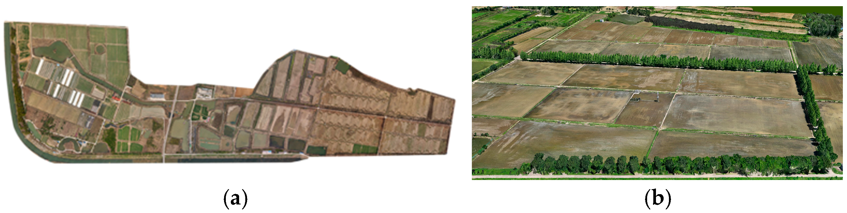
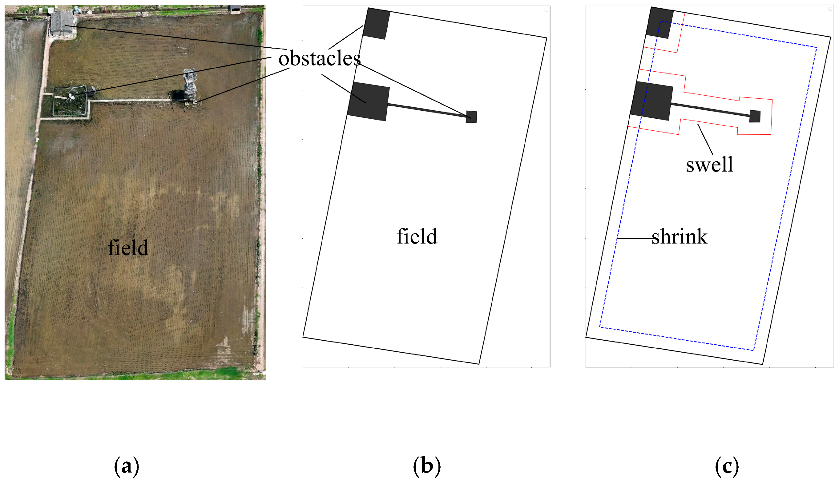
2.1. Three-Dimensional Field Reconstruction and Boundary Buffering

A DJI UAV equipped with an onboard RGB camera was deployed to acquire low-altitude imagery for 3D field reconstruction. The selected study area was the Houbaix Farm, located at a longitude of 119.21° and a latitude of 31.81°. After acquisition, the imagery was processed via the DJI Terra platform(DJI Terra platform, version 4.5.0; DJI, Shenzhen, China). The full workflow included feature point extraction, image alignment, point cloud reconstruction, surface modeling, and texture mapping. A high-resolution 3D model was eventually generated, as illustrated in Figure 1. The derived digital elevation model (DEM) and digital orthophoto map (DOM) provided accurate geospatial references for field boundary delineation, obstacle identification, and coverage path planning.

After completing the 3D reconstruction, the Tuxin Earth platform (v4.0; SinoGNSS (Suzhou) Technology Co., Ltd., Suzhou, China) was used to extract field boundaries and obstacle distribution information. Special attention was given to identifying key geographic features such as field corner points and obstacle edges, which provided essential input for subsequent path planning. The initially extracted spatial data were represented in the WGS-84 coordinate system. However, since WGS-84 is a geodetic (spherical) coordinate system and cannot be directly used for accurate distance and angle calculations, a coordinate transformation was required. The data were first converted to the Earth-centered, Earth-fixed (ECEF) coordinate system and then further transformed into the local east–north–up (ENU) coordinate frame [33], which was more suitable for local planar computations in path planning tasks.

Given a point with geodetic coordinates $(\varphi ,\lambda ,h)$, where $\varphi$ is latitude, $\lambda$ is longitude, and $h$ is ellipsoidal height, its corresponding Earth-centered, Earth-fixed (ECEF) coordinates can be expressed as

$$\left\{\begin{array}{c}X=\left(N+h\right)·\cos \left(\varphi \right)·\cos \left(\lambda \right)\\ Y=\left(N+h\right)·\cos \left(\varphi \right)·\sin \left(\lambda \right)\\ Z=\left(N·\left(1-e^2\right)+h\right)·\sin \left(\varphi \right)\end{array}\right.$$

(1)

Here, $N$ is the prime vertical radius of curvature, calculated by:

$$N={\displaystyle \frac{\sigma }{\sqrt{1-e^2{\sin }^2(\varphi )}}}$$

(2)

where $e^2$ is the first eccentricity squared of the reference ellipsoid, $\sigma$ is the semi-major axis of the reference ellipsoid.

For local path-planning, the target point must be expressed in a topocentric frame that is centered on a chosen reference location. The ECEF coordinates $\left(X,Y,Z\right)$ obtained from Equation (1) are therefore translated and rotated with respect to the reference point $(X_0,Y_0,Z_0)$. The resulting east–north–up (ENU) coordinates $(E,N,U)$ are given by

$$\left[\begin{array}{c}E\\ N\\ U\end{array}\right]=\left[\begin{array}{ccc}-\sin \left({\lambda }_0\right)& \cos \left({\lambda }_0\right)& 0\\ -\sin \left({\varphi }_0\right)·\cos \left({\lambda }_0\right)& -\sin \left({\varphi }_0\right)·\sin \left({\lambda }_0\right)& \cos \left({\varphi }_0\right)\\ \cos \left({\varphi }_0\right)·\cos \left({\lambda }_0\right)& \cos \left({\varphi }_0\right)·\sin \left({\lambda }_0\right)& \sin \left({\varphi }_0\right)\end{array}\right]\left[\begin{array}{c}X-X_0\\ Y-Y_0\\ Z-Z_0\end{array}\right]$$

(3)

Let $({\varphi }_0,{\lambda }_0)$ denote the latitude and longitude of the reference point, and $(X_0,Y_0,Z_0)$ be its ECEF coordinates. The final local displacements $(E,N,U)$, obtained using Equations 1–3, represent the offsets from the reference origin in the east, north, and up directions, respectively.

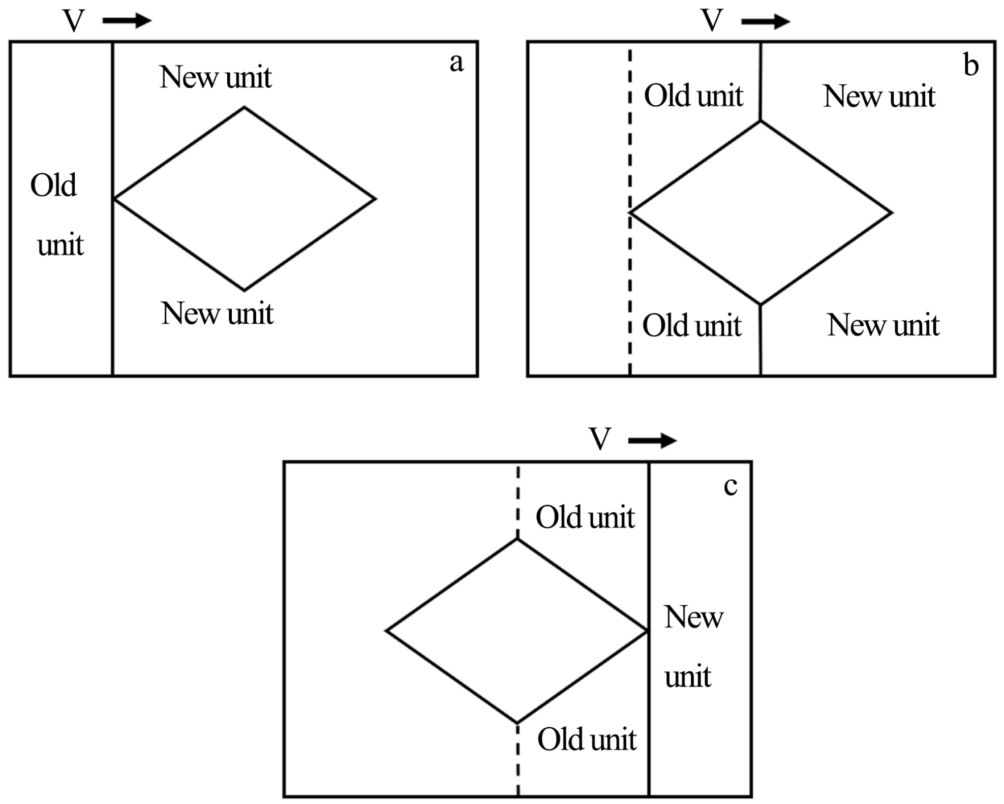
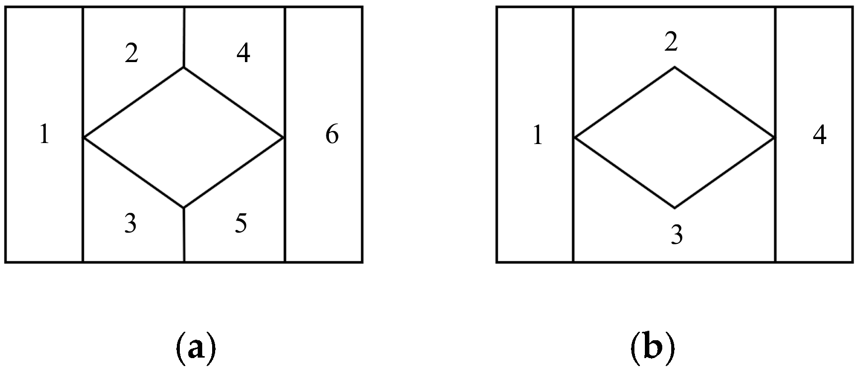
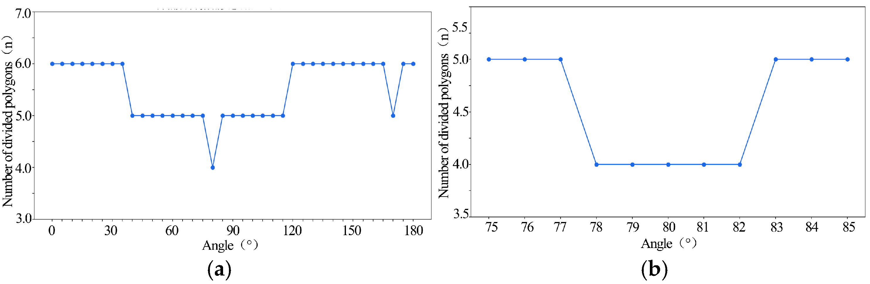
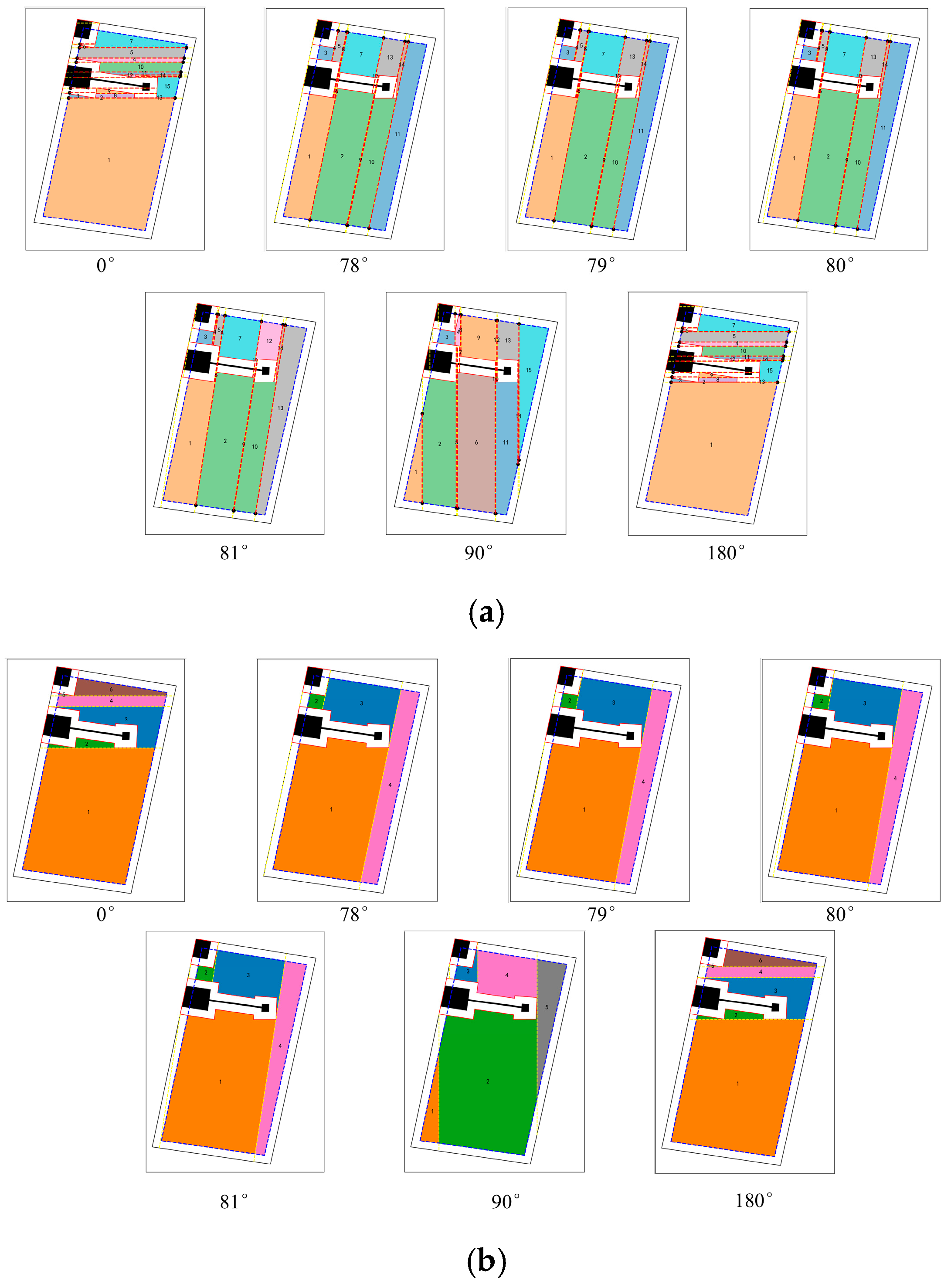
2.2. Target Area Segmentation

Prior to path planning, the field boundaries are contracted inward, and obstacle boundaries are expanded outward using a polygon-offsetting method (Clipper2 library [31]). This operation leaves a buffer zone that prevents collisions and coverage gaps. In this study the offset distance is calculated as

$$d_{\mathrm{buf}}=\max (R_{\min },0.5d)+m_{gnss}$$

(4)

This rule follows headland-width recommendations in curvature-constrained CPP studies [34]: the buffer must be at least the larger of the turning radius or half the implement width. Because Equation (4) involves only three platform-specific parameters, it can be re-parameterized rapidly for different vehicles, thereby enhancing path continuity and operational safety.

Subsequently, appropriate area segmentation is applied to further improve operational efficiency. By optimizing both the partition angle and spatial layout, the method minimizes the number of sub-regions while maintaining regularity in shape. This contributes to simplifying the subsequent path planning, reducing travel distances, and lowering the number of turns, thereby laying a solid data foundation for path generation and task scheduling.

Among field partitioning methods, the trapezoidal decomposition approach is commonly adopted, as illustrated in Figure 2. Its core idea is to use a vertically moving sweep line from left to right, triggering three types of events upon intersecting obstacle vertices: an IN event indicates entry into an obstacle and splits the area into two sub-regions, a MIDDLE event indicates crossing the middle of an obstacle and generates one sub-region, and an OUT event indicates leaving the obstacle and reduces the number of active regions. By continuously handling these events, the original region can be decomposed into multiple regular and obstacle-free trapezoidal cells [35], which facilitates the subsequent path planning.

An enhanced version of this method, known as the boustrophedon decomposition, further optimizes the process. It also employs vertical sweep lines but only triggers segmentation when intersecting with obstacle edge vertices, omitting unnecessary intermediate cuts [36]. This strategy significantly reduces the number of decomposition units, as shown in Figure 3b.

To standardize calculations, the parameters defined in

Table 1. Definitions of key geometric and planning parameters used in field segmentation and path generation.

Parameter Name	Symbol	Unit
Sub-region width (long side)	$w$	m
Working width	$d$	m
Safety allowance accounting for GNSS error	$m_{gnss}$	m
Minimum turning radius of agricultural machine	$R_{\min }$	m
The offset distance	$d_{\mathrm{buf}}$	m
Angle between path and field boundary	$\alpha$	°
Segmentation angle	$\theta$	°
Path planning angle	${\theta }_c$	°

were used. Within each sub-region, the boustrophedon decomposition method generated parallel back-and-forth working paths, commonly referred to as boustrophedon trajectories in agricultural operations. Given a path interval (working width) $d$ and a sub-region width $w$, the machine proceeded back and forth at regular intervals of $d$ until the entire region was covered. The coverage trajectory can be expressed as

$$y_i=y_0+i\cdot d,i\in \{0,1,\dots ,[w/d]\}$$

(5)

where $y_0$ is the initial position, and $y_i$ is the position of the $i$ path line.

To overcome the limitation of conventional boustrophedon-based path segmentation methods that only support fixed orientations (such as vertical or horizontal), a user-controllable segmentation angle configuration is introduced. The working direction can be flexibly defined within the range of 0° to 180°, rather than being restricted to a single fixed direction. By adaptively adjusting the segmentation angle, the path planning process can dynamically align with the shape of field boundaries, terrain features, and the operational orientation of the agricultural machinery. This significantly enhances the flexibility of path generation and improves overall coverage efficiency. The improvement is particularly beneficial in complex fields with irregular boundaries or fixed internal obstacles, where it markedly strengthens the adaptability and effectiveness of autonomous agricultural operations.

To this end, the traditional sweeping model equation was modified. Assuming that the field was partitioned based on a specified orientation angle (see Figure 4), the corresponding coverage path can be described mathematically as follows:

$$i\cdot d=y_i-tan\left(\theta \right)\cdot x_i,i\in \left\{0,1,\dots ,\left[w/d\right]\right\}$$

(6)

where $\theta$ is the segmentation angle.

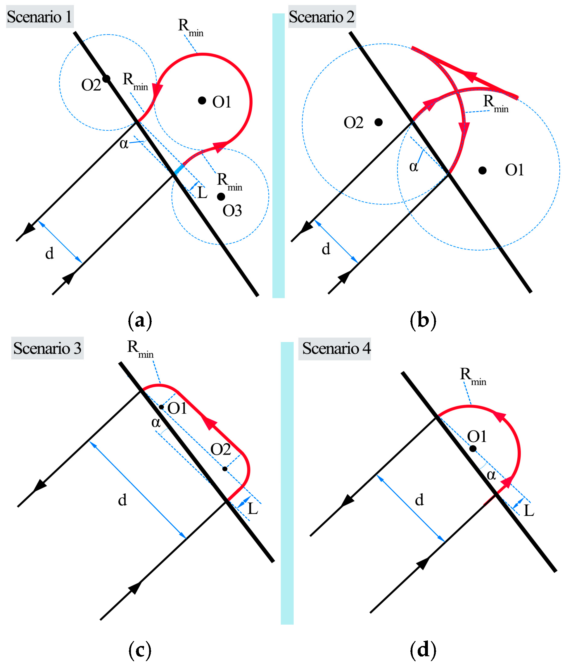
2.3. Sub-Region Coverage Path Planning

In field operations, agricultural machinery often requires prior knowledge of performance parameters and the geometric information of the working area. Based on field boundaries, the minimum turning radius, and the working width, a rational planning strategy can be developed to coordinate path generation and turning behaviors. Among various approaches, straight-line-based planning methods are widely applied due to their operational simplicity and high efficiency. This section focuses on the planning of straight working paths and explores strategies for further optimization.

The core objectives of path planning include reducing the number of turns to lower operational complexity, minimizing total path length to save time and energy, and improving overall task efficiency. Traditional methods typically adopt a fixed-direction strategy for partitioning, which performs well in regular fields. However, when dealing with irregular plots or fields with special operational requirements, such rigid planning may result in path overlaps, incomplete coverage, or excessive turning frequency [37]. To address these challenges, a rotation-based direction adjustment mechanism is introduced. This mechanism allows the path direction to be flexibly configured based on the field’s geometry and actual operational constraints. As a result, both path adaptability and quality are significantly improved. Let the boundary of the field be defined as $Q=\{(x_1,y_1),(x_2,y_2),...,(x_n,y_n)\}$. Given a sweeping distance $d$ and a specified planning direction ${\theta }_c$, the field boundary is first rotated by an angle ${\theta }_c$ (to align the path direction with the x-axis). The transformation is expressed as

$$\left[\begin{array}{c}{x}^{\prime }\\ y^{\prime }\end{array}\right]=\left[\begin{array}{cc}\cos \left(-{\theta }_c\right)& -\sin \left(-{\theta }_c\right)\\ \sin \left(-{\theta }_c\right)& \cos \left(-{\theta }_c\right)\end{array}\right]\left[\begin{array}{c}x-x_c\\ y-y_c\end{array}\right]+\left[\begin{array}{c}{x}_c\\ y_c\end{array}\right]$$

(7)

Here, $(x_c,y_c)$ is the rotation center (usually the centroid of the field polygon), ($x,y$) are the original coordinates, and ($x^{\prime },y^{\prime }$) are the rotated coordinates.

Next, the sweeping lines are generated according to the following equation:

$$y_u=y_{\mathrm{a}}+u\cdot d,u\in \{0,1,\dots ,w/d\}$$

(8)

where $y_{\mathrm{a}}$ is the starting coordinate, and $u$ denotes the index of the $u$-th sweeping line.

To ensure evenly spaced waypoints and improve trajectory smoothness, linear interpolation is performed at fixed intervals between adjacent points. Given a starting point and an endpoint, intermediate points are inserted along the straight line connecting them.

Given a starting point $p_{n0}(x_{n0},y_{n0})$ and an ending point $p_{n1}(x_{n1},y_{n1})$, the Euclidean distance between them is calculated as

$$d_n=\sqrt{{(x_{n1}-x_{n0})}^2+{(y_{n1}-y_{n0})}^2}$$

(9)

The interpolated point coordinates are then computed as

$$x_{li}=(1-t)x_{n0}+t{x}_{n1},y_{li}=(1-t)y_{n0}+t{y}_{n1}$$

(10)

To determine the coordinates of interpolated points along a segment, the interpolation factor $t$ is defined as

$$t={\displaystyle \frac{s\times \mathrm{interval}}{d_n}},s=1,2,...,\mathrm{steps}$$

(11)

where $\mathrm{interval}$ is the fixed step length, $d_n$ is the total distance between two endpoints, and $s$ is the index of the interpolated point. In addition to spacing control, it is also necessary to calculate turning directions between adjacent path segments. The turning direction is determined using the vector cross product method as follows:

Let the current path segment end at point $P_0(m_0,n_0)$, with a previous point $P_1(m_1,n_1)$, and the next path segment starting at point $P_2(m_2,n_2)$.

Then, the direction vector of the previous path is

$${\overrightarrow{v}}_1=\left(m_1-m_0,n_1-n_0\right)$$

(12)

The direction vector of the next path is

$$\overrightarrow{v_2}=\left(m_2-m_1,n_2-n_1\right)$$

(13)

The cross product of the direction vectors ${\overrightarrow{v}}_1\times {\overrightarrow{v}}_2$ is computed as

$${\overrightarrow{v}}_1\times {\overrightarrow{v}}_2=\left(m_1-m_0\right)\left(n_2-n_1\right)-\left(n_1-n_0\right)\left(m_2-m_1\right)$$

(14)

Using the sign of the two-dimensional cross product to distinguish left and right turns is a classical predicate in computational geometry [38]. The result of the cross product indicates the turning direction:

$$\left\{\begin{array}{ccc}\overrightarrow{v_1}\times \overrightarrow{v_2}>0& ,& turn-left\\ \overrightarrow{n_1}\times \overrightarrow{n_2}<0& ,& turn-right\\ \overrightarrow{n_1}\times \overrightarrow{n_2}=0& ,& go-straight\end{array}\right.$$

(15)

Once the turning direction at the end of each path segment is determined, the next step is to specify the corresponding turning strategy. Fish-tail turns, teardrop turns, semi-circular turns, and arc-shaped turns are among the most commonly used maneuvers in agricultural operations. Referring to the agricultural turning path planning method proposed by Wang Meng and considering the minimum turning radius of the machine $R_{\min }$, the angle $\alpha$ between the field boundary and the perpendicular to the working line at the headland, as well as the working width $d$, the characteristics of the four turning types are illustrated in Figure 5.

The pear-shaped turning path $S_p$ primarily consists of two clothoid segments with a minimum radius $R_{\min }$ and one semicircular arc also with radius $R_{\min }$. The clothoids connect the semicircle smoothly with the two straight working paths. Throughout the entire turning maneuver, the machine maintains forward motion without stopping or reversing. The total turning path length is given by

$$S_p=(\pi +4\arccos {\displaystyle \frac{d+2R_{\min }}{4R_{\min }}})R_{\min }+d\tan \alpha$$

(16)

The fish-tail turning path $S_f$ consists of two circular arcs with radius $R_{\min }$ and one straight-line segment. The arcs are tangent to the straight section, and the machine transitions smoothly from the turning path to the next working line. The total path length is calculated as

$$S_f=\pi R_{\min }+\sqrt{{(2R_{\min }-d)}^2+{(d\tan \alpha )}^2}$$

(17)

The arc-shaped turning path $S_g$ is composed of two circular arcs of radius $R_{\min }$ and one straight-line segment. The arcs are tangent to both the working paths and the straight-line connection. The machine moves forward throughout the maneuver. The total path length is given by

$$S_g=(\pi -2)R_{\min }+(1+\tan \alpha )d$$

(18)

The semi-circular turning path $S_h$ consists of a single semicircle with radius $R_{\min }$, tangent to both working lines. The machine moves forward during the entire turn. The path length is

$$S_h=\pi R_{\min }+d\tan \alpha$$

(19)

Taking a rectangular field as an example, different turning strategies are evaluated. When the minimum turning radius $R_{\min }⩽{\displaystyle \frac{d}{2}}$, neither fish-tail nor pear-shaped turning methods can be applied due to geometric constraints, and semi-circular turns are typically adopted. When $R_{\min }>{\displaystyle \frac{d}{2}}$, although fish-tail and pear-shaped turns become geometrically feasible, arc-based turning is often preferred due to its simplicity and avoidance of reversing maneuvers. Thus, arc-shaped turns are selected as the standard turning method for modeling and optimization in this study.

Assume the machine starts at point $(m_0,n_0)$, with an initial heading angle ${\theta }_0$. The goal is to execute a turn along a circular arc with minimum turning radius $R_{\min }$ and a central turning angle $\mathsf{\Delta }\theta$. When the machine transitions from a straight line into a circular arc, the arc’s center $(x_c,y_c)$ is determined by the initial point and turning direction:

$$\begin{array}{l}{x}_c=\left\{\begin{array}{c}{m}_0-R_{\min }\sin ({\theta }_0),leftturn\\ m_0+R_{\min }\sin ({\theta }_0),rightturn\end{array}\right.\\ y_c=\left\{\begin{array}{c}{n}_0+R_{\min }\cos ({\theta }_0),leftturn\\ n_0-R_{\min }\cos ({\theta }_0),rightturn\end{array}\right.\end{array}$$

(20)

To generate smooth arc trajectories, a sequence of interpolation points along the circular arc of radius $R_{\min }$ is computed as

$$\begin{array}{c}{x}_i=x_c+R_{min}\cos ({\theta }_0+i\cdot \mathsf{\Delta }\theta /N)\\ y_i=y_c+R_{min}\sin ({\theta }_0+i\cdot \mathsf{\Delta }\theta /N)\end{array}$$

(21)

where $i=0,1,...,N$ is the sampling index, and N is the number of interpolation points (the higher, the smoother the arc).

To systematically evaluate and compare different path planning strategies across multiple dimensions, a weighted comprehensive scoring method is adopted in this study. First, each performance indicator is directionally unified and normalized using the Min–Max method. Then, a weighted sum is calculated to obtain the overall score $S$, where a lower score indicates better overall performance. The calculation process is as follows:

$$m_i^{\mathrm{norm}}={\displaystyle \frac{m_i-m_{\min }}{m_{\max }-m_{\min }}},(m\in \{N_{\mathrm{turn}},L_{\mathrm{path}},R_{\mathrm{dup}},T_{\mathrm{plan}}\})$$

(22)

$$S=w_1{N}_{\mathrm{turn}}^{\mathrm{norm}}+w_2{L}_{\mathrm{path}}^{\mathrm{norm}}+w_3{R}_{\mathrm{dup}}^{\mathrm{norm}}+w_4{T}_{\mathrm{plan}}^{\mathrm{norm}}$$

(23)

Here, $m_i^{\mathit{norm}}$ denotes the normalized value of metric m. The evaluation indicators include the following: The assessment includes four key indicators: the number of turns $N_{\mathit{turn}}$, total path length $L_{\mathit{path}}$, coverage redundancy rate $R_{\mathit{dup}}$, and planning time $T_{\mathit{plan}}$. Each metric is assigned a weight $w_1,w_2,w_3,w_4$, based on its relative importance. The sum of all weights satisfies the condition $\sum w_j=1$.

2.4. Sub-Region Traversal Planning

This section introduces a multi-subregion traversability planning strategy for agricultural fields. The algorithm seeks to generate the shortest closed-loop path across all subregions, under the constraint of a minimum turning radius and a fixed safety distance from obstacles. It integrates 8-directional A* search, polyline simplification, circular arc smoothing, Chaikin subdivision, and cubic B-spline interpolation to generate continuous and efficient inter-subregion paths.

To accommodate GNSS positioning errors and ensure sufficient clearance for agricultural machinery, a fixed-width safety buffer $d_{\mathit{safe}}$ is applied around both field boundaries and obstacles. The entire working area is denoted as a polygon $P$, with obstacles represented by the set ${\left\{O_j\right\}}_{j=1}^m$ and the target subregions by ${\left\{F_i\right\}}_{i=1}^n$. Using morphological dilation, the expanded unsafe zone $\tilde{O}$ is constructed as

$$\tilde{O}={\displaystyle \underset{j=1}{\overset{m}{\cup }}(O_j\oplus B_{d_c})}\cup {\displaystyle \underset{i=1}{\overset{n}{\cup }}\left((P\backslash F_i)\oplus B_{d_c}\right)}$$

(24)

Here, $B_{d_{\mathrm{safe}}}=\{x\in {ℝ}^2\mid \parallel x\parallel \le d_{\mathrm{safe}}\}$ denotes a circular buffer of radius $d_{\mathit{safe}}$, and the symbol ⊕ represents the Minkowski sum, which is used to dilate obstacle boundaries outward by the specified safe margin. After computing the buffered region $\tilde{O}$, the valid traversable region $\mathsf{\Omega }$ is defined by subtracting it from the overall area:

$$\mathsf{\Omega }=P\backslash \tilde{O}$$

(25)

The traversable workspace is then discretized into a grid map with resolution $\mathsf{\Delta }r$, resulting in a binary traversability matrix $G(i,j)\in \{0,1\}$ of dimensions $N_r\times N_c$:

$$G(i,j)=\left\{\begin{array}{ll}0,& (x_{ij},y_{ij})\in \mathsf{\Omega },\\ 1,& \mathrm{otherwise},\end{array}\right.$$

(26)

The spatial coordinates $(x_{ij},y_{ij})$ remapped to grid indices $(i,j)$ as follows:

$$\begin{array}{l}i=\left({\displaystyle \frac{y_{ij}-y_{\min }}{\mathsf{\Delta }r}}\right),\\ j=\left({\displaystyle \frac{x_{ij}-x_{\min }}{\mathsf{\Delta }r}}\right)\end{array}$$

(27)

To determine the shortest traversable route from the current subregion $S_k$ of the entry point $E_{k+1}$ of the next subregion, an 8-directional A* search algorithm is applied over the grid matrix $G$. For each step, horizontal and vertical movements are assigned a cost of 1, while diagonal steps are assigned a cost of $\sqrt{2}$. The evaluation function for a node $p$ is defined as

$$\begin{array}{l}f(p)=g(p)+h(p),\\ h(p)=\max (\left|i_p-i_g\right|,\left|j_p-j_g\right|)\end{array}$$

(28)

Here, $g(p)$ denotes the actual cost from the start node to the current node $p$, while $h(p)$ is the heuristic cost estimating the remaining distance to the goal node. Indices $i_p$$j_p$ represent the corresponding indices of the goal node. The A* output is a grid-based polyline path, which typically exhibits a step-wise shape that is not ideal for machinery trajectory execution. To generate a smooth and feasible driving path, the polyline is post-processed using a multi-stage refinement pipeline consisting of simplification, arc-based corner smoothing, Chaikin subdivision, and B-spline interpolation.

As the first step, the raw path is simplified using the Douglas–Peucker algorithm with a tolerance parameter varepsilonε, which is generally set to match the GNSS resolution. The simplified polyline path $P^{\ast }$ is defined as

$$P^{\ast }=\mathrm{DP}(V,\epsilon )$$

(29)

where $V$ is the original point set output by A*, and $P^{\ast }$ is the reduced set of waypoints after simplification. For any three consecutive simplified points $(P_{k-1},P_k,P_{k+1})$, the turning angle ${\theta }_k$ between three consecutive simplified waypoints is calculated as

$${\theta }_k=\arccos {\displaystyle \frac{\left(P_{k-1}-P_k\right)\cdot \left(P_{k+1}-P_k\right)}{\parallel P_{k-1}-P_k\parallel \parallel P_{k+1}-P_k\parallel }}$$

(30)

If a circular arc of radius R is to be inserted at the turning corner, the arc length parameter $d_k$ is computed as

$$d_k={\displaystyle \frac{R}{\tan ({\theta }_k/2)}}\le \min \{\parallel P_{k-1}-P_k\parallel ,\parallel P_{k+1}-P_k\parallel \}$$

(31)

When this condition is satisfied, the corner is replaced with a smooth circular arc of length $d_k$. Next, the polyline is subjected to $s$ iterations of Chaikin subdivision, during which each segment $(P_k^{(t-1)},P_{k+1}^{(t-1)})$ is replaced by two new control points:

$$\begin{array}{c}{Q}_k^{(t)}={\displaystyle \frac{3}{4}}{P}_k^{(t-1)}+{\displaystyle \frac{1}{4}}{P}_{k+1}^{(t-1)},\\ R_k^{(t)}={\displaystyle \frac{1}{4}}{P}_k^{(t-1)}+{\displaystyle \frac{3}{4}}{P}_{k+1}^{(t-1)},t=1,\dots ,s,\end{array}$$

(32)

The resulting control point set is interpolated using cubic B-spline curves to yield a smooth and continuous trajectory:

$$B(u)=\sum _{i=0}^m{N}_{i,3}\left(u\right)P_i,0\le u\le 1$$

(33)

where $N_{i,3}\left(u\right)$ denotes the i-th cubic B-spline basis function.

To determine the optimal subregion traversal sequence, a traveling salesman problem (TSP) is solved based on A* distance estimates. Let each subregion ${\pi }_k$ have an endpoint $E_{{\pi }_k}$ and an entry point $S_{\pi k+1}$. For a candidate traversal sequence $\pi =({\pi }_1,{\pi }_2,...,{\pi }_n)$, the total loop cost is defined as

$$J(\pi )=\sum _{k=1}dist\left(E_{{\pi }_k},S_{{\pi }_{k+1}}\right),S_{{\pi }_{n+1}}=S_{{\pi }_1}$$

(34)

where $\mathrm{dist}(·,·)$ is the minimum feasible distance between subregion exit and entry points, estimated via the A* search algorithm defined in Equation (27). To ensure that the traversal path forms a closed loop, the start point of the first subregion is connected to the endpoint of the last one, enforcing $S_{{\pi }_{n+1}}=S_{{\pi }_1}$. All $n!$ permutations are exhaustively evaluated to determine the traversal order ${\pi }^{*}$ that minimizes the total loop cost:

$${\pi }^{*}=arg\underset{\pi }{min}J\left(\pi \right)$$

(35)

By applying Equations (23)–(34), the proposed framework ensures subregion coverage paths that are smooth, continuous, and globally optimized for both safety margins and minimal travel distance.

3. Results

3.1. Construction of 2D Field Map and Geometric Preprocessing

To evaluate the applicability and effectiveness of the proposed algorithm in real-world scenarios, a case study was conducted at Houbai Farm, located in Jurong, China (longitude 119.21°, latitude 31.81°). A high-resolution digital elevation model (DEM) of the area was obtained through UAV-based 3D reconstruction. Based on this, simulation experiments were conducted. Field boundary and obstacle data were manually annotated point by point using the Tuxin Earth platform, enabling accurate extraction of spatial geometry.

The field boundary was defined by the polygon with vertices at (0.0, 0.0), (38.494, −5.468), (53.313, 60.52), and (14.28, 66.615). As illustrated in Figure 6a, the selected field featured irregular boundaries and included four obstacles of varying shapes. The black rectangular outline delineates the outer boundary of the field, encompassing a total area of 2654.20 m². The solid black polygons denote the obstacles, with individual areas ranging from 5.30 m² (smallest) to 57.57 m² (largest). To reduce geometric complexity, three intersecting obstacles were merged into a single composite object, resulting in a combined area of 68.41 m². This simplification enhanced the efficiency of subsequent region partitioning and path planning.

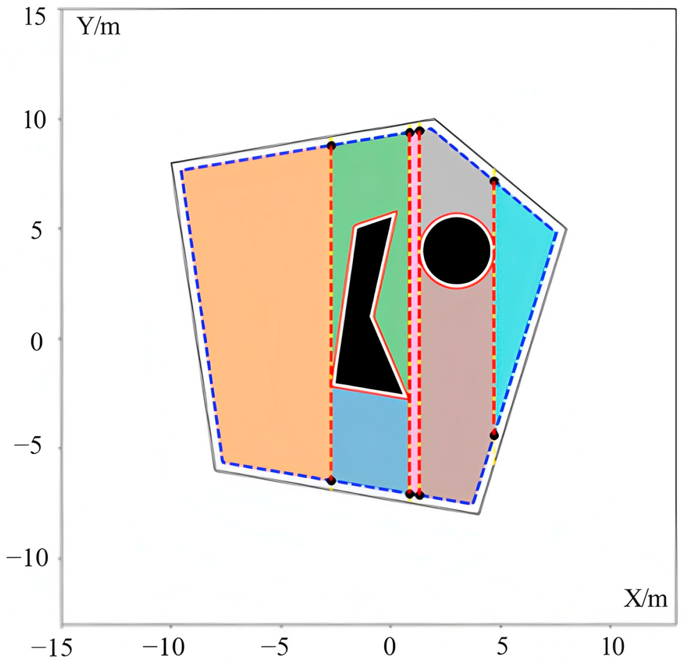
3.2. Field Partitioning

To ensure sufficient space for maneuvering and obstacle avoidance, a 3 m inward offset was applied to the field boundary based on the minimum turning radius of the agricultural machinery. Simultaneously, each obstacle boundary was expanded outward by 3 m to establish a safe operating buffer zone. These geometric modifications were implemented using the Clipper library. The processed results are illustrated in Figure 6c. The blue dashed lines represent the contracted field boundary, while the red solid lines denote the expanded obstacle boundaries.

To evaluate the effectiveness of boustrophedon partitioning under different angular configurations, a series of field segmentation experiments were conducted using various division angles. The segmentation results were subsequently compared with those generated using the conventional trapezoidal decomposition method.

In complete coverage path planning, the number of turns and the total path length directly affect operational efficiency. To investigate how the segmentation angle influences path layout, tests were performed at 5° intervals across the range of 0° to 180°. As shown in Figure 7a, the smallest number of subregions was obtained when the division angle approached 80°. This reduction in segmentation frequency was favorable as it lowered the number of inter-subregion transitions and thus reduced the overall turning costs.

Building on the preliminary findings, a finer analysis was conducted by narrowing the angle range to 75–85°, with a resolution of 1° (see Figure 7b). The results indicated that within the interval of 78° to 81°, the field could be consistently divided into four subregions, reflecting a more favorable segmentation outcome. Therefore, this angle range was selected for further investigation, focusing on coverage path performance to identify the optimal segmentation angle.

In addition to the four selected angles with superior performance, three conventional segmentation angles—0°and 90°—were included for comparison as baseline references. As shown in Figure 8b, the boustrophedon-based method produced significantly fewer subregions than the traditional trapezoidal decomposition (Figure 8a), highlighting its advantage in reducing segmentation complexity.

These results demonstrate that in complex environments with irregular field boundaries and internal obstacles, the boustrophedon-based segmentation method offers a more effective approach for optimizing regional partitioning. It significantly reduces path overlap and mitigates the problem of region fragmentation.

3.3. Coverage Path Planning Simulation

To evaluate the suitability of segmentation angles ranging from 78° to 81° for coverage path planning, a series of simulation experiments were conducted. For each subregion, the working direction $\theta$ was varied across the full 0–360° range in 5° increments. At each orientation, key path performance metrics were computed, including the number of turns, total path length, overlap rate, and planning time.

The weighting scheme for these metrics was determined based on their impact on fuel consumption and operation time. Specifically, the number of turns and total path length were each assigned a weight of 0.40. This decision was supported by the Fields2Cover benchmark dataset, which showed that 0.5% to 50% of the total travel distance was typically consumed by turning maneuvers and that redundant straight-line travel could increase task duration by 22% to 28% [25]. In addition, field tillage trials revealed that an additional 0.14 h·ha⁻¹ of non-operational travel could consume up to 0.85 kg·ha⁻¹ of fuel [39]. The overlap rate was assigned a weight of 0.10. Although its influence was secondary, GNSS-based field measurements suggested that even a 6–11% overlap could lead to more than 20% wastage of input resources [40]. Planning time was also weighted at 0.10 as it typically accounts for less than 1% of total operation time in modern CPP systems [41].

To ensure meaningful comparisons, all path planning outcomes were required to achieve a minimum coverage rate of 98%. Under the above constraints, a weighted composite scoring method was used to evaluate each solution. Notably, the weight vector $[w_1,w_2,w_3,w_4]$ in Equation (22) is not fixed. Users may redefine the weights according to specific priorities in different scenarios—such as spray uniformity, real-time navigation, or energy optimization. The proposed framework supports user-defined weighting through a flexible interface, following the same normalization and scoring process.

Figure 9a–d illustrate the relationship between the working direction and the composite score for the four selected fields under each segmentation angle. Based on the results, the 78° segmentation scheme was ultimately selected as the optimal planning strategy.

The simulation results indicated that among all candidate segmentation angles, the 78° configuration achieved the most favorable overall performance. This angle aligned more closely with the geometric contours of the field, resulting in subregion boundaries that were more regular and compact. Such geometric conformity effectively reduced unnecessary turns and redundant paths, thereby enhancing the overall efficiency of path planning.

For the buffered field polygon (see Figure 6c), when an infinitely long sweep line $L_{\theta }$ oriented at angle $\theta$ moved from left to right, each time $L_{\theta }$ crossed a boundary vertex it triggered an IN/OUT event (see Table 1 for definitions and Figure 2 for event types). Let each polygon edge have outward normal angle $L_i$. The number of subregion strips can be approximated as follows (derivation adapted from [1]):

$$E(\theta )={\displaystyle \frac{1}{2d}}\sum _{i=1}^n\left|\sin (\theta -{\phi }_i)\right|L_i$$

(36)

This expression implies that when $\theta$ is parallel to most edges (especially the longest ones), $\left|\sin (\theta -{\phi }_i)\right|$ approaches zero, minimizing $E(\theta )$ and thus yielding the fewest subregions. For the test field the longest edge lies at 77.9°. Hence, 78° simultaneously minimizes both the number of sub-regions and their shape irregularity, consistent with the empirical sweep in Figure 10.

Based on 78° segmentation, the initial working directions for the four subregions were set to 255°, 165°, 80°, and 260° (see Figure 9). To further optimize directional alignment, a refined search was conducted around these initial directions with a step size of 1°. The optimized working orientations were adjusted to 258°, 161°, 78°, and 260°. These improvements led to enhanced performance in coverage operations, with detailed results summarized in

Table 2. Performance metrics of three CPP methods.

Planner	Coverage Rate (%)	Number of Turns	Path Length (m)	Planning Time (s)	Overlap Rate (%)
Angle-adaptive (ours)	99.97	21	897.19	0.0225	0.00
Belief-space	99.24	32	1164.00	0.052	0.00
Bidirectional spiral	92.23	93	1044.00	0.043	1.11

.

Comparing the 78° segmentation in Table 2 with the conventional 0°/90° schemes in

Table 3. Simulation results under 0° and 90° segmentation angles with 0° and 90° heading angles.

Segmentation Angle (°)	Heading Angle (°)	Coverage Rate (%)	Number of Turns	Path Length (m)	Planning Time (s)	Overlap Rate (%)
90	0	99.14	71	1167.48	0.1561	2.21
	90	98.04	32	1056.17	0.0722	0
0	0	98.74	32	1069.17	0.0716	0.20
	90	99.41	81	1209.96	0.1496	8.25

confirms its benefits: coverage rose by 0.4–0.8 percentage points, turn count dropped by 55–70%, path length shortened by 8–23%, and planning time fell by 54–86%. Table 3 also shows that while the belief-space CPP attained similar coverage, it still required 32 turns, a 1164 m path, and 0.052 s of computation; the bidirectional spiral was faster but left 7.8% of the area uncovered, produces 1.11% overlap, and relies on 93 turns over 1044 m. These comparisons highlight the geometric and computational advantages of the proposed angle-adaptive planner.

After determining the optimal segmentation angle and working direction for each of the four subregions, an integrated coverage path planning simulation was performed. The resulting full-field coverage layout is illustrated in Figure 11a, where the planned paths reflect the optimal division and direction strategy for each individual field.

In addition, the operation paths across all subregions were seamlessly merged into a unified coverage plan. Through simulation-based extraction, the entry and exit coordinates for each subregion were identified. The results are presented in

Table 4. Entry and exit coordinates of field plots.

Plot ID	Entry Coordinates	Exit Coordinates
1	(3.796, 2.492)	(29.615, −1.09)
2	(18.771, 56.08)	(18.362, 54.106)
3	(43.323, 58.591)	(22.039, 50.847)
4	(34.147, −1.88)	(48.798, 58.171)

, serving as critical input for subsequent inter-field connection and global routing optimization.

In this experiment, four subfields (labeled 1–4) were selected, with the initial starting point set at field 1’s entrance located at coordinates (29.615, −1.09). Following the algorithmic workflow described in Section 2.4, the initial inter-field connection paths were generated using an eight-directional A* search on a 0.10 m resolution occupancy grid. This raw polyline output was then sequentially refined through a series of post-processing steps: polyline simplification using the Douglas–Peucker algorithm with tolerance ε = 1.5 m, arc-based corner smoothing with a minimum radius of 1.0 m, and Chaikin subdivision and cubic B-spline interpolation for final smoothing. The resulting transition paths are shown in Figure 11c.

Under constraints ensuring safe buffer margins and adherence to the machinery’s minimum turning radius, a brute-force TSP (travelling salesman problem) enumeration approach was employed to determine the optimal visiting sequence. The resulting order was 1 → 4 → 3 → 2. In Figure 11, green circles indicate subfield entry points, red circles denote exits, and colored solid lines represent the inter-field transition trajectories.

Table 5. Core parameter settings.

Parameter	Value	Parameter	Value
Clearance (m)	1.5	Turn threshold (°)	30
Grid resolution (m)	0.1	RDP Epsilon (ε)	1.5
Corner radius (m)	1.0	Tolerance (TOL)	0.9
Corner samples	3	Max radius filter	25
Chaikin iterations	1

summarizes the key planning parameters used in this simulation. Additionally, the transition performance between subfields is quantitatively evaluated across four metrics: distance, average curvature radius, number of sharp turns, and number of path steps, with detailed results presented in

Table 6. Path transition planning results.

Segment	Distance (m)	Avg Radius (m)	Turns	Steps
1 → 4	5.04	5.48	1	69
4 → 3	66.55	11.06	2	785
3 → 2	7.76	5.12	1	84
2 → 1	98.47	8.77	6	1126
Total	177.81	7.61	10	2064

.

4. Discussion

This study presents a novel path planning framework for agricultural fields with fixed obstacles, integrating 3D perception, angle-adaptive boustrophedon partitioning, and multi-segment closed-loop path generation [42]. Unlike conventional boustrophedon approaches with fixed 0° or 90° orientations, the proposed method employed a two-level angular search (5° coarse and 1° fine steps) over the 0–360° range. The results demonstrated that the 78–81° interval yielded the most stable and efficient partitioning, consistently dividing the target area into four regular subregions. Among these, the 78° segmentation strategy achieved superior results, increasing coverage to 99.97%, while reducing the number of turns by up to 70.42%, path length by 23.17%, and computation time by 85.6%. These improvements substantiated the hypothesis that adaptive segmentation angles significantly enhanced path efficiency. A multi-metric weighted evaluation scheme (weights 0.40, 0.40, 0.10, and 0.10) further confirmed the integrated benefits of the proposed segmentation–planning strategy in terms of energy saving and operational efficiency. The framework also supports user-defined weight customization, enabling flexible optimization based on scenario-specific priorities. Moreover, using eight-directional A* search combined with a polyline-arc-Chaikin-B-spline smoothing pipeline, the total transition distance between subregions was controlled within 177.81 m, with an average curvature radius of 7.61 m—ensuring both path continuity and maneuverability.

A major strength of this framework lies in its applicability to irregular fields without requiring idealized terrain assumptions. Nonetheless, two limitations remain: The framework relies heavily on high-precision GNSS data, limiting its adaptability in occluded or dynamic environments. Smoothness parameters and indicator weights require manual tuning based on specific machine models and task requirements, preventing full automation.

Future research will focus on the following directions: (1) Field validation across diverse conditions: Conduct multi-season and multi-soil-moisture field trials to evaluate fuel efficiency and productivity gains under different crop types and operational environments. (2) Scalable multi-machine coordination: Develop auction-based task allocation or reinforcement learning strategies to enable cooperative planning and load balancing for large-scale farms, further reducing total operation time. (3) Energy-aware path modeling: Incorporate slope and traction resistance models into the path evaluation process, advancing toward joint optimization of trajectory and energy consumption for more sustainable and low-carbon agricultural operations. (4) Adaptive planning in dynamic environments: Integrate real-time obstacle detection and SLAM techniques, introducing probabilistic maps and incremental replanning to improve adaptability in occluded or changing conditions. To operationalize this vision we will build an ROS 2 pipeline in which 3-D LiDAR clustering and CNN-based vision are fused into a real-time stream of tracked objects. The resulting velocity-labeled targets are injected, via a time-decaying dynamic-obstacle layer, into the Nav2 cost-map that underlies both global coverage planning and local D*-Lite replanning. When an inflated cost exceeds a safety threshold, the vehicle either generates a short detour inside the current lane or temporarily skips the blocked strip, while a bitmap merger ensures that unfinished areas are revisited once the obstruction disappears.

References

1. Wang, M. Research on Key Technologies of Task Allocation for Multi-Machine Cooperative Operation of Agricultural Machinery. Ph.D. Thesis, Chinese Academy of Agricultural Mechanization Sciences, Beijing, China, 2021. [Google Scholar]
2. Luo, R.; Gan, X.; Yang, G. A full-coverage path planning method for autonomous agricultural machinery with obstacle avoidance. J. Agric. Mech. Res. 2025, 47, 36–43. [Google Scholar] [CrossRef]
3. Zhu, S.; Wang, B.; Pan, S.; Ye, Y.; Wang, E.; Mao, H. Task allocation of multi-machine collaborative operation for agricultural machinery based on the improved fireworks algorithm. Agronomy 2024, 14, 710. [Google Scholar] [CrossRef]
4. Zeng, Y. Research on Full-Coverage Path Planning for Sugarcane Harvester in Irregular-Shaped Fields. Master’s Thesis, Guangxi University, Nanning, China, 2024. [Google Scholar]
5. Choset, H.; Pignon, P. Coverage path planning: The boustrophedon cellular decomposition. In Field and Service Robotics; Springer: London, UK, 1998; pp. 203–209. [Google Scholar]
6. Kuang, W.; Ho, H.W.; Zhou, Y. CPP-DIP: Multi-objective coverage path planning for MAVs in dispersed and irregular plantations. arXiv 2025, arXiv:2505.04989. [Google Scholar]
7. Liang, J.; Liu, L. Optimal path planning method for unmanned surface vehicles based on improved shark-inspired algorithm. J. Mar. Sci. Eng. 2023, 11, 1386. [Google Scholar] [CrossRef]
8. Han, J.; Li, W.; Xia, W.; Wang, F. Research on complete coverage path planning of agricultural robots based on Markov chain improved genetic algorithm. Appl. Sci. 2024, 14, 9868. [Google Scholar] [CrossRef]
9. Wang, X.; Nie, T.; Zhu, D. Indoor robot path planning assisted by wireless network. J. Wirel. Com. Netw. 2019, 2019, 123. [Google Scholar] [CrossRef]
10. Yang, L.; Li, P.; Wang, T.; Miao, J.; Tian, J.; Chen, C.; Tan, J.; Wang, Z. Multi-area collision-free path planning and efficient task scheduling optimization for autonomous agricultural robots. Sci. Rep. 2024, 14, 18347. [Google Scholar] [CrossRef]
11. Lu, E.; Xu, L.Z.; Li, Y.M.; Tang, Z.; Ma, Z. Modeling of working environment and coverage path planning method of combine harvesters. Int. J. Agric. Biol. Eng. 2020, 13, 132–137. [Google Scholar] [CrossRef]
12. Chen, T.; Xu, L.; Ahn, H.S.; Lu, E.; Liu, Y.; Xu, R. Evaluation of headland turning types of adjacent parallel paths for combine harvesters. Biosyst. Eng. 2023, 233, 93–113. [Google Scholar] [CrossRef]
13. Cui, B.; Cui, X.; Wei, X.; Zhu, Y.; Ma, Z.; Zhao, Y.; Liu, Y. Design and testing of a tractor automatic navigation system based on dynamic path search and a fuzzy Stanley model. Agriculture 2024, 14, 2136. [Google Scholar] [CrossRef]
14. Zhang, F.; Teng, S.; Wang, Y.F.; Guo, Z.J.; Wang, J.J.; Xu, R.L. Design of bionic goat quadruped robot mechanism and walking gait planning. Int. J. Agric. Biol. Eng. 2020, 13, 32–39. [Google Scholar] [CrossRef]
15. Zhu, X.Y.; Chikangaise, P.; Shi, W.D.; Chen, W.H.; Yuan, S.Q. Review of intelligent sprinkler irrigation technologies for remote autonomous system. Int. J. Agric. Biol. Eng. 2018, 11, 23–30. [Google Scholar] [CrossRef]
16. Kong, F.; Qiu, B.; Dong, X.; Yi, K.; Wang, Q.; Jiang, C.; Zhang, X.; Huang, X. Design and development of a side spray device for UAVs to improve spray coverage in obstacle neighborhoods. Agronomy 2024, 14, 2002. [Google Scholar] [CrossRef]
17. Shang, G.; Liu, G.; Han, J.; Zhu, P.; Chen, P. Research on full-coverage path planning algorithm for horticultural electric tractors. J. Agric. Mech. Res. 2022, 44, 35–40. [Google Scholar] [CrossRef]
18. Zoto, J.; Musci, M.A.; Khaliq, A.; Chiaberge, M.; Aicardi, I. Automatic Path Planning for Unmanned Ground Vehicle Using UAV Imagery. In Advances in Service and Industrial Robotics; Berns, K., Görges, D., Eds.; Advances in Intelligent Systems and Computing; Springer International Publishing: Cham, Switzerland, 2020; Volume 980, pp. 223–230. [Google Scholar] [CrossRef]
19. Zhang, H.; Li, Q.; Feng, L. Assessing the Severity of Verticillium Wilt in Cotton Fields and Constructing Pesticide Prescription Maps Using UAV Multispectral Images. Drones 2023, 8, 176. [Google Scholar] [CrossRef]
20. Liu, C.Q.; Zhao, X.Y.; Du, Y.F.; Cao, C.; Zhu, Z.; Mao, E. Research on static path planning method of small obstacles for automatic navigation of agricultural machinery. IFAC-Pap. Online 2018, 51, 748–753. [Google Scholar] [CrossRef]
21. Schirmer, R.; Biber, P.; Stachniss, C. Coverage path planning in belief space. In Proceedings of the 2019 IEEE International Conference on Robotics and Automation (ICRA), Montreal, QC, Canada, 20–24 May 2019; pp. 7604–7610. [Google Scholar]
22. Lu, Q.; Luna, R. Adaptive multiple distributed bidirectional spiral path planning for foraging robot swarms. In Proceedings of the 2023 20th Conference on Robots and Vision (CRV), Montreal, QC, Canada, 6–8 June 2023; pp. 225–232. [Google Scholar] [CrossRef]
23. Ahmed, S.; Qiu, B.; Ahmad, F.; Kong, C.-W.; Xin, H. A state-of-the-art analysis of obstacle avoidance methods from the perspective of an agricultural sprayer UAV’s operation scenario. Agronomy 2021, 11, 1069. [Google Scholar] [CrossRef]
24. Kharel, T.; Owens, P.; Ashworth, A. Tractor path overlap is influenced by field shape and terrain attributes. Agric. Environ. Lett. 2020, 5, e20027. [Google Scholar] [CrossRef]
25. Mier, G.; Valente, J.; de Bruin, S. Fields2Cover: An open-source coverage path planning library for unmanned agricultural vehicles. IEEE Robot. Autom. Lett. 2023, 8, 2436–2443. [Google Scholar] [CrossRef]
26. Chen, W.; Yang, J.; Zhang, S.; Wei, X.; Liu, C.; Zhou, X.; Sun, L.; Wang, F.; Wang, A. Variable scale operational path planning for land levelling based on the improved ant colony optimization algorithm. Sci. Rep. 2025, 15, 9854. [Google Scholar] [CrossRef]
27. Mansur, H.; Gadhwal, M.; Abon, J.E.; Flippo, D. Mapping for Autonomous Navigation of Agricultural Robots Through Crop Rows Using UAV. Agriculture 2025, 15, 882. [Google Scholar] [CrossRef]
28. Gao, C.; Wang, S.; Hu, J.; Liang, Y. Planning method of field road network reconstruction under mechanized farming mode. J. Xihua Univ. (Nat. Sci. Ed.) 2024, 43, 45–54. [Google Scholar]
29. Liu, H. Research on Development of Automatic Driving Equipment and Path Planning Algorithm for Agricultural Machinery. Master’s Thesis, North University of China, Taiyuan, China, 2023. [Google Scholar]
30. Yang, L.; Tang, X.; Wu, S.; Wen, L.; Yang, W.; Wu, C. Local path planning for autonomous agricultural machinery on field roads. Trans. Chin. Soc. Agric. Eng. 2024, 40, 27–36. [Google Scholar]
31. Höffmann, M.; Patel, S.; Büskens, C. Optimal coverage path planning for agricultural vehicles with curvature constraints. Agriculture 2023, 13, 2112. [Google Scholar] [CrossRef]
32. Li, J.; Shang, Z.; Li, R.; Cui, B. Adaptive sliding mode path tracking control of unmanned rice transplanter. Agriculture 2022, 12, 1225. [Google Scholar] [CrossRef]
33. Cui, Z.; Li, Y.; Zhang, C.; Liu, Y.; Ren, F. Coarse-to-fine 3D road model registration for traffic video augmentation. IET Image Process. 2020, 14, 2690–2700. [Google Scholar] [CrossRef]
34. Oksanen, T.; Visala, A. Coverage path planning algorithms for agricultural field machines. J. Field Robot. 2009, 26, 651–668. [Google Scholar] [CrossRef]
35. Kim, C.; Kim, Y.; Yi, H. Fuzzy analytic hierarchy process-based mobile robot path planning. Electronics 2020, 9, 290. [Google Scholar] [CrossRef]
36. Liu, Y.; Geng, D.; Lan, Y.; Tan, D.; Mou, X.; Sun, Y. Research progress on full-coverage path planning of agricultural equipment based on automatic navigation. Chin. J. Agric. Mech. 2020, 41, 185–192. [Google Scholar]
37. Nan, F.; Cao, G.; Li, Y.; Chen, C.; Liu, D. Research on scheduling optimization based on walking direction of wheat harvester operation routes. Chin. J. Agric. Mech. 2022, 43, 98–105. [Google Scholar]
38. de Berg, M.; van Kreveld, M.; Overmars, M.; Schwarzkopf, O. Computational Geometry: Algorithms and Applications, 3rd ed.; Springer: Berlin, Germany, 2008; pp. 5–8. [Google Scholar]
39. Damanauskas, V.; Janulevičius, A. Validation of criteria for predicting tractor fuel consumption and CO2 emissions when ploughing fields of different shapes and dimensions. AgriEngineering 2023, 5, 2408–2422. [Google Scholar] [CrossRef]
40. Kaivosoja, J.; Linkolehto, R. Spatial overlapping in crop farming works. Agron. Res. 2016, 14, 41–53. Available online: https://api.semanticscholar.org/CorpusID:54953705 (accessed on 10 March 2025).
41. Collins, L.; Ghassemi, P.; Esfahani, E.T.; Doermann, D.; Dantu, K.; Chowdhury, S. Scalable coverage path planning of multi-robot teams for monitoring non-convex areas. In Proceedings of the 2021 IEEE International Conference on Robotics and Automation (ICRA), Xi’an, China, 30 May–5 June 2021; pp. 7393–7399. [Google Scholar] [CrossRef]
42. Ahmed, S.; Qiu, B.; Kong, C.-W.; Xin, H.; Ahmad, F.; Lin, J. A data-driven dynamic obstacle avoidance method for liquid-carrying plant protection UAVs. Agronomy 2022, 12, 873. [Google Scholar] [CrossRef]
Figure 1. Three-dimensional field reconstruction results of the Houbaix Farm using DJI UAV imagery(DJI Mavic 3 Pro UAV; DJI, Shenzhen, China). (a) Overall 3D reconstruction. (b) Local detail showing terrain and field edge features.
Agriculture 15 01479 g001
Figure 2. Schematic diagram of obstacle event classification and handling in trapezoidal decomposition. (a) IN event: the sweep line enters an obstacle, resulting in the division of the region into two new sub-regions. (b) MIDDLE event: the sweep line crosses through the middle of an obstacle, generating one additional sub-region. (c) OUT event: the sweep line exits the obstacle, reducing the number of active sub-regions.
Agriculture 15 01479 g002
Figure 3. Comparison of unit partitioning strategies: (a) Trapezoidal decomposition (units numbered 1–6 in generation order). (b) Boustrophedon-based decomposition (units numbered 1–4 in generation order).
Agriculture 15 01479 g003
Figure 4. Schematic diagram of buffer zone incorporation and path division. Blue dashed line: inner-offset boundary (buffer zone); red solid line: obstacle inflation boundary; red dashed lines: segmentation lines.
Agriculture 15 01479 g004
Figure 5. Illustration of four typical turning maneuvers commonly adopted in agricultural path planning. (a) Pear-shaped turn. (b) Fish-tail turn. (c) Bow-shaped turn. (d) Half-circle turn.
Agriculture 15 01479 g005
Figure 6. Field boundary extraction and obstacle buffering results. (a) Real-world UAV image of the study area. (a) Real-world UAV image of the study area. (b) Initial boundary and obstacle annotation. (c) Visualization of the 3 m inward contraction and outward expansion buffer zones.
Agriculture 15 01479 g006
Figure 7. Influence of segmentation angle on the number of divided sub-regions. (a) Sub-region count variation with 5° segmentation angle intervals from 0° to 180°. (b) Refined analysis using 1° intervals from 75° to 85°.
Agriculture 15 01479 g007
Figure 8. Effects of two decomposition strategies at different segmentation angles. (a) Trapezoidal decomposition results under various representative angles. (b) Boustrophedon-based decomposition results under the same angles. Color coding: White areas indicate navigable workspace, black polygons denote obstacles, the black solid outline shows the original field boundary, the blue dashed outline corresponds to the inward-buffered boundary, the red solid outline depicts the obstacle-expansion boundary, and red (or white) dashed lines mark segmentation lines between sub-regions. Colored fills (orange, green, blue, pink, grey, and teal) distinguish individual trapezoidal sub-regions Numbers label each sub-region in generation order (1 = first sub-region, 2 = second sub-region, etc.).
Agriculture 15 01479 g008
Figure 9. Composite evaluation scores for path planning under different heading angles across four test fields. Subplots show performance for (a) field 1, (b) field 2, (c) field 3, and (d) field 4.
Agriculture 15 01479 g009
Figure 10. Comparison of coverage results under 0° and 90° segmentation conditions with different path orientations. (a) Path planning result at 0° segmentation with 0° path orientation. (b) Path planning result at 0° segmentation with 90° path orientation. (c) Path planning result at 90° segmentation with 0° path orientation. (d) Path planning result at 90° segmentation with 90° path orientation. Red shaded areas indicate uncovered regions. Lines in different colors indicate the coverage trajectories for each sub-region.
Agriculture 15 01479 g010
Figure 11. Multi-field operation planning: simulation and sequence optimization results. (a) Complete coverage path layout for individual sub-fields. (b) Unsmoothed coverage paths in each sub-field. (c) Optimized inter-field routing and traversal order. Thick red lines indicate the traversal route for each sub-region.
Agriculture 15 01479 g011