Tracking Accuracy Evaluation of Autonomous Agricultural Tractors via Rear Three-Point Hitch Estimation Using a Hybrid Model of EKF Transformer

Abstract

The objective of this study was to improve measurement accuracy in the evaluation of autonomous agricultural tractor performance by addressing external disturbances, such as sensor installation errors, vibrations, and heading-induced bias that occur during the measurement of the conventional rear three-point hitch (Rear 3-Point) system. To mitigate these disturbances, the measurement point was relocated to the cab, where external interference is comparatively minimal. However, in compliance with the ISO 12188 standard, the Rear 3-Point system must be used as the reference measurement point. Therefore, its coordinates were indirectly estimated using an extended Kalman filter (EKF) and artificial intelligence (AI)-based techniques. A hybrid model was developed in which a transformer-based AI model was trained using the Rear 3-Point coordinates predicted by EKF as the ground truth. While traditional time-series models, such as LSTM and GRU, show limitations in predicting nonlinear data, the application of an attention mechanism was found to enhance prediction performance by effectively learning temporal dependencies and vibration patterns. The experimental results show that the EKF-based estimation achieved a precision of RMSE 1.6 mm, a maximum error of 12.6 mm, and a maximum standard deviation of 3.9 mm compared to actual measurements. From the perspective of experimental design, the proposed hybrid model was able to predict the trajectory of the autonomous agricultural tractor with significantly reduced external disturbances when compared to the actual measured Rear 3-Point coordinates, while also complying with the ISO 12188 standard. These findings suggest that the proposed approach provides an effective and integrated solution for developing high-precision autonomous agricultural systems.

1. Introduction

In recent years, the agricultural sector has been making various efforts to address issues such as population growth, climate change, and labor shortages. In the study conducted by [1] the potential of autonomous agricultural machinery as a means to achieve objectives pertaining to the enhancement of productivity and the sustainability of agricultural operations was analyzed. The study emphasized the need to integrate robots and autonomous agricultural machinery, a necessity arising from the diminishing workforce of skilled agricultural laborers in aging societies. Ref. [2] emphasized that robotics and autonomous machinery technology are core solutions to structural issues, such as the aging of the agricultural population and labor shortages. The authors also introduced recent cases of the application of these technologies to various agricultural tasks (e.g., sowing, harvesting, and pest management).

“Asia’s agricultural sector: A comprehensive analysis”, found that although the continent accounts for approximately 67% of the world’s farms, the average farm size in Asia is only 1.2 to 2.8 hectares [3]. In the context of a diminutive farmstead, the inability of autonomous agricultural machinery to accurately estimate its position has the potential to result in a number of issues, including boundary violations, duplicate work, and edge omissions. It is evident that ensuring the procurement of high-precision autonomous driving technology for small farm units is a fundamental prerequisite for the successful implementation of automation processes.

Presently, research is being conducted on the development of high-precision autonomous agricultural machinery. An analysis revealed the potential of these technologies to enhance work efficiency and safety [4]. This enhancement is achieved through the utilization of technologies such as precise location recognition, path planning and tracking, and motion control. A low-cost autonomous driving system equipped with GNSS and inertial sensors was developed [5]. This system was then demonstrated to achieve high driving precision with a path-following error of 0.10 m in an actual orchard environment. An intelligent unmanned agricultural machinery system integrating location recognition, path planning, and driving control technologies was developed [6]. This system was then demonstrated to have precise driving control and high work efficiency through actual vehicle experiments. A vehicle positioning method that applies ultra-wideband (UWB)-based cooperative positioning technology and a Bayesian integration algorithm to overcome the limitations of global navigation satellite systems (GNSS) was proposed [7]. The validity of this method was demonstrated through experiments that yielded centimeter-level accuracy.

In accordance with Korean certification standards for autonomous tractors, it is necessary to ensure that the cumulative 95% value of path-following error falls within 7 cm, in accordance with the relevant Korean regulations [8]. The evaluation of this parameter is achieved by measuring the error between the actual driving path and the planned path, whilst the tractor follows the planned path. At the Korean Agricultural Machinery Testing Institute [9], a planned path (A-B line) is set, and the target agricultural machinery is driven along the path. The positions of the Rear 3-Points are measured using a total station prism system to obtain coordinates. The sensors installed on Rear 3-Points are subject to various disturbances, including vibration, installation position, and steering-induced skewing, which is problematic. Various disturbance factors, such as tractor vibration, inclination, and sensor noise, can degrade measurement accuracy, and active research is being conducted to suppress these effects [10]. In their study, IMU-based filtering and correction algorithms were employed to minimize the influence of such disturbances, thereby improving the reliability of measurements through experimental validation. Due to traceability limitations inherent in standardized measurement procedures, the use of GNSS- or IMU-based sensors was restricted. To compensate for this constraint and minimize the effects of disturbances, such as vibration and installation errors, the measurement coordinates were relocated to the cab point, which is relatively less affected by such factors, in order to ensure measurement accuracy.

The objectives of this study are as follows:

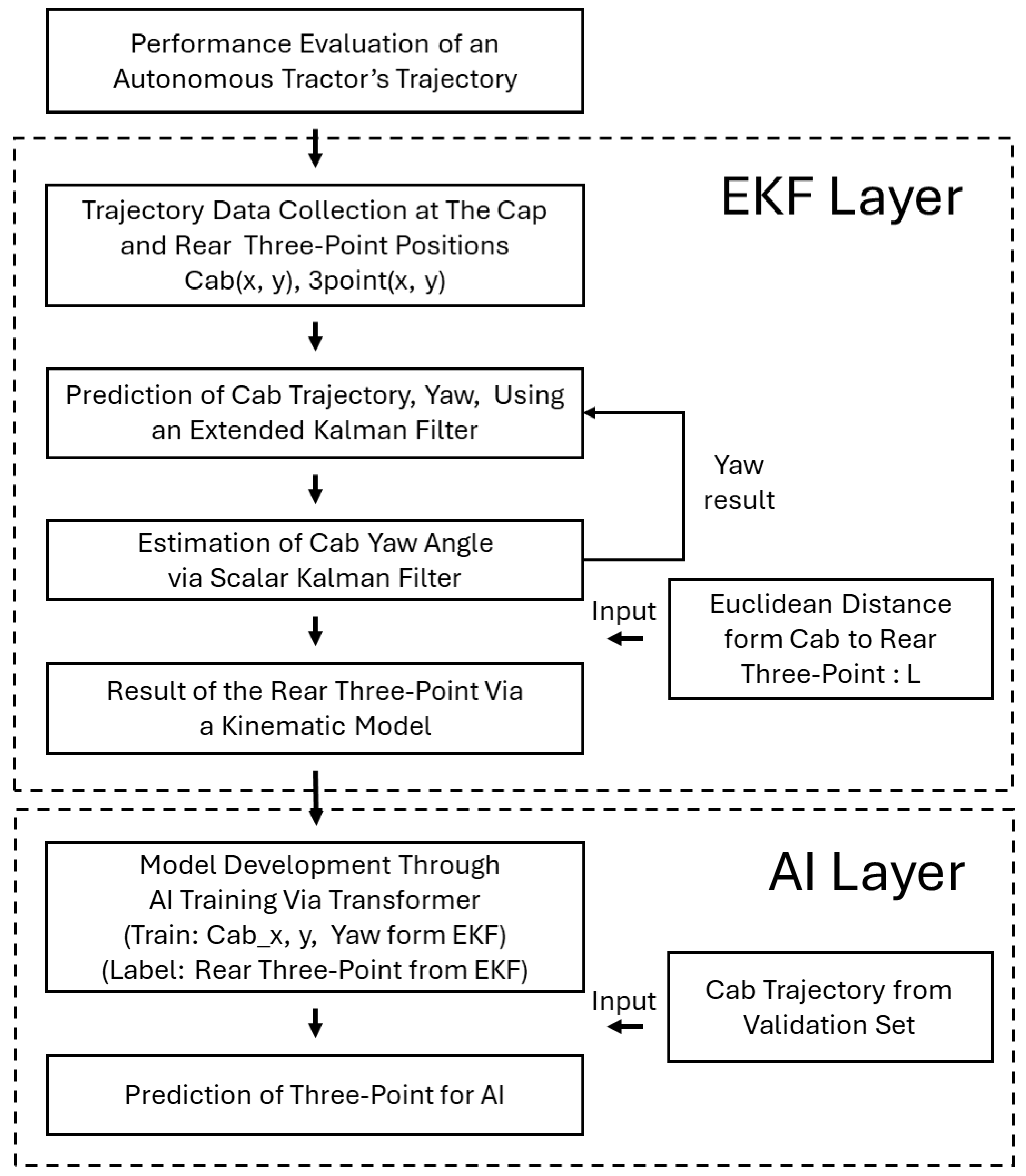
• The development of a hybrid model combining an extended Kalman filter (EKF) and an artificial intelligence-based transformer for the purpose of tracking the Rear 3-Point device of a tractor is presented in this study.
• A demonstration test was conducted, and a comparative analysis of the hybrid model was undertaken to enhance the autonomous driving path-following capability.

2. Materials and Methods

2.1. Prediction Model Development Procedure

The experimental procedure for estimating the Rear 3-Point using a hybrid model of the extended Kalman filter and an AI-based attention transformer is shown in Figure 1. The coordinates of the Rear 3-Point and the yaw angle were estimated using the extended Kalman filter (EKF) based on the kinematic model. A two-layer modeling architecture was adopted, in which the extended Kalman filter (EKF) was first applied to generate pseudo-ground-truth trajectories under noisy conditions. Subsequently, an attention-based transformer model was trained on these estimates to learn the temporal relationships between cab sensor inputs and the Rear 3-Point trajectories, effectively capturing long-range and nonlinear dynamics within the time-series data. The measurement coordinates of the cab point were used to mitigate observation noise. The yaw predicted by the EKF was corrected using a scalar Kalman filter to compensate for yaw drift. The objective of this procedure was to estimate the coordinates of the Rear 3-Point support points reliably, based on cab position information, with disturbances removed. Subsequently, the cab coordinate values, the yaw predicted by the EKF, and the relative distance information between the cab sensor position and the Rear 3-Points were used as input values. The continuously estimated coordinates of the Rear 3-Point were utilized as label values in the training of an attention-based transformer model. In conclusion, the system was configured to predict the position of Rear 3-Point solely using the continuously measured cab position values. In their 2020 paper, A hybrid AI model that integrates vehicle lane change intention classification and trajectory prediction [11]. The study employed an artificial neural network (ANN) to categories vehicle steering intentions and utilized an LSTM-based time-series model to predict future positions. This approach yielded an RMS lateral error of approximately 0.30 m in real-road scenarios. The present study finds itself in alignment with extant research insofar as it also adopted AI for the purpose of trajectory analysis. However, it should be noted that there are two key differences between this approach and the others discussed. Firstly, the study is conducted in a simulation environment, which is subject to inherent limitations. Secondly, and more fundamentally, it adopted a different approach to implementing AI during algorithm design. Transformer-based models exhibit performance that is comparable to or better than recurrent models, such as LSTM and GRU, particularly under conditions involving irregular noise and alignment uncertainty [12,13]. In this context, the present study adopted a transformer architecture to model the temporal characteristics of Rear 3-Point trajectories, rather than relying on conventional RNN-based approaches. The selection was made in consideration of the transformer’s ability to process long-range dependencies and handle nonlinear vibration patterns in time-series data. Furthermore, its parallel processing capability offered practical advantages in terms of learning efficiency and model scalability. Accordingly, the transformer model was trained using the cab position, EKF-estimated yaw angle, and relative distance vectors as inputs, with the estimated Rear 3-Point positions serving as output labels.

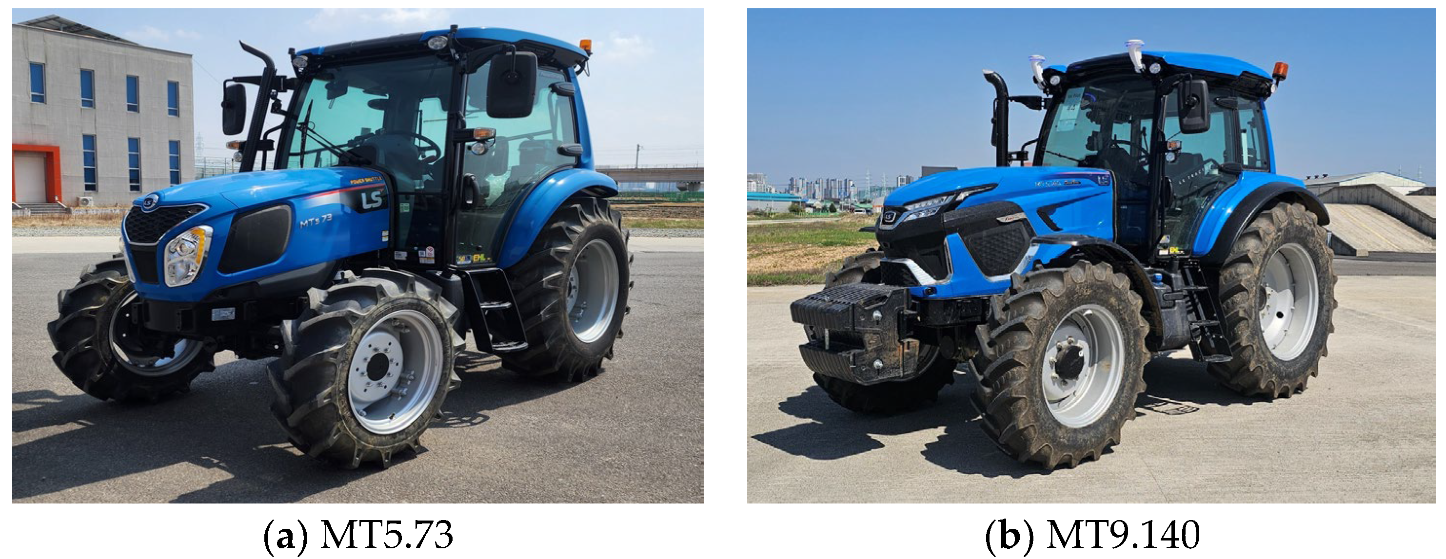
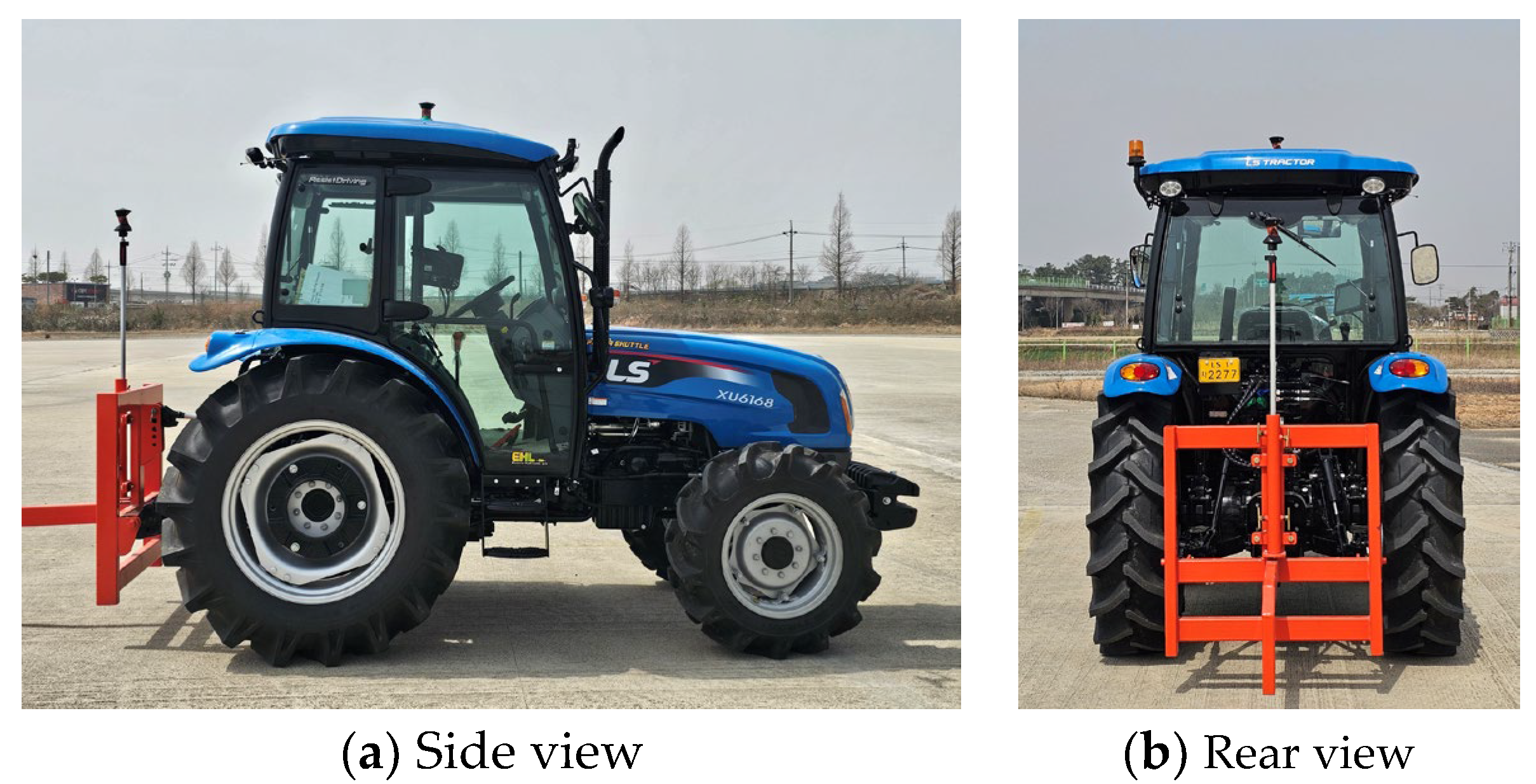
2.2. Agricultural Tractor and Autonomous Driving System

In this study, the autonomous tractors employed were models with specifications of 47 kW (2300 rpm) (MT5.73, LSMtron Co., Ltd., Wanju, Republic of Korea) and 89 kW (2300 rpm) (MT9.140, LSMtron Co., Ltd., Wanju, Republic of Korea) (Figure 2). The tractor specifications are outlined in

Table 1. Specifications of the autonomous agricultural tractors.

Item		Specifications
		MT5.73	MT9.140
Length × Width × Height (mm)		3900 × 1900 × 2780	4600 × 2300 × 2930
Weight (kg)		3065	5330
Steering System Type		Fully Hydraulic	Fully Hydraulic
Wheelbase (mm)		2150	2600
Track Width (mm)	Front Wheel	1590	1890
	Rear Wheel	1435	1800
Tire Specifications	Front Wheel	11.2–24 8PR	380/85 R28
	Rear Wheel	16.9–30 8PR	460/85 R38
Autonomous Control System	Input Steering Interval (Hz)	100	5
	Max. Steering Angle (Degree)	45	37
GNSS	Sampling Frequency (Hz)	10	50
	RTK-GPS Accuracy (mm)	15	20

. It is evident that both tractors successfully completed the requisite tests for power take-off (PTO) output, traction force, and lifting force, with the exception of autonomous driving. It is worth noting that both tractors have been approved under the OECD Tractor Code.

The autonomous steering of the MT5.73 and MT9.140 agricultural tractor models uses an RTK-GPS (GPS receiver, Ascen, Geumcheongu, Republic of Korea) with a precision of 20 mm. The MT5.73 model uses a 100 Hz specification actuator motor (Jinan Keya Electron Science Technology Co., Ltd., Jinan, People’s Republic of China), while the MT9.140 uses a 5 Hz model (Block-STR_V/V, Limsco Co., Ltd., Goyang, Republic of Korea). Each model also employs different autonomous driving system modules. The wheelbase, track width, and other specifications also differ between the two models.

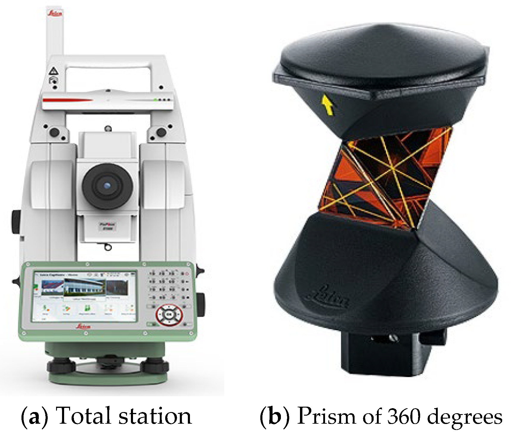
2.3. Total Station and Prism

In this study, the trajectory measurement instrument utilized a total station with a precision of 2 mm and a continuous measurement cycle of 10 Hz (TS13, Leica Geosystems AG, Heerbrugg, Switzerland), as specified in

Table 2. Specification of total station in this study.

Item	Specification
Measurement range (mm)	0.9 m to 3500 m
Accuracy (mm)	1 mm (1.5 PPM)
Measurement interval (hz)	10
Working temperature range (°C)	−20 to +50

and Figure 3. The adopted coordinate system follows the azimuth-of-a-line convention. Two reflective prisms were installed in parallel, at arbitrary points, as shown in Figure 3, with the direction of the autonomous driving path designated as the x-axis.

In this study, the driving trajectory of an autonomous agricultural tractor was tracked with great precision. To this end, 360-degree reflective prisms were affixed to the cabin and the Rear 3-Point, as shown in Figure 4. The prisms were then aligned with the vertical centerline of the agricultural tractor, as shown in Figure 3. In the case of the Rear 3-Point support prism installation, visual inspection of minor installation errors in the left–right direction from the vertical centerline was challenging due to the link structure. In the event of the center alignment of the test device being inaccurate, an increase in measurement deviations may be observed. the position deviation of the implement is significantly influenced by the rotation of the tractor and terranin roughness as confirmed in [14]. This finding indicates that the initial position uncertainty of the agricultural tractor results in substantial lateral deviations throughout the experiment.

2.4. Testing Field and Planned Trajectory

The field experiment was carried out at the agriculture machinery driving test facility in May 2025. The test site for the autonomous agricultural tractor under investigation was located at the driving test site in Iksan, Republic of Korea, as shown in Figure 5a. The test site comprised a flat concrete surface with an average slope of 1 cm or less, as shown in Figure 5b. The experiment was conducted under clear weather conditions on a dry surface. The C-type work pattern was identified as the most representative work pattern, with reference to its extensive utilization in practical applications [15]. In this study, the continuous trajectory of the cab and three-point support points was measured by driving along the C-type work pattern path shown in Figure 5c. Furthermore, the K-type work pattern was utilized to augment the heterogeneity of the experiment. This method has been adopted by previous studies as a representative tilling technique and can be utilized in experimental scenario design that reflects actual working conditions. The autonomous driving speed was set to 0.3 m/s for MT5.3 (low speed 1st gear) and 0.2 m/s for MT9.140 (ultra-low speed 1st gear) with the throttle fully open. According to ISO 12188-1, 2, evaluations must be conducted at low, medium, and high speeds, with the low-speed condition defined as 0.1 ± 0.05 m/s or the lowest speed supported by the system [16,17]. Therefore, the test speeds applied in this study were in compliance with the ISO low-speed criteria. Furthermore, based on the performance test results provided by the Korea Agricultural Technology Promotion Agency, these speeds correspond to conditions under which the largest path-following errors were observed. Therefore, the selected test speeds reflect the worst-case scenario in terms of trajectory accuracy.

2.5. EKF and Transformer Model Development Methods

2.5.1. Data Preprocessing and Independent Variable Analysis

In this study, we collected continuous coordinates (trajectories) of two different models of agricultural tractors (MT5.73 and MT9.140) as they traveled along a planned route. In order to evaluate straightness in accordance with the international standard ISO 12188 and the Korean agricultural machinery evaluation method, it was necessary to exclude the 10-m sections before and after turns. Furthermore, in order to facilitate data comparison, the driving direction was not corrected, and solely the coordinate origin (0, 0) was adjusted as the reference point. The data obtained for each model are presented in

Table 3. Data classification according to agriculture tractor model.

Model	1st Line	2nd Line	3rd Line	4th Line
MT5.73	EKF-AI train	EKF-AI train	Validation (Using raw data)	EKF-AI train
MT9.140	EKF-AI train	Validation (Using raw data)	EKF-AI train	EKF-AI train

, where the third straight-line run of MT5.73 and the second run of MT9.140 were utilized for validation.

2.5.2. Correction of Time-Series Misalignment and Coordinate Normalization

It is evident that minor discrepancies in the time series of measurement data are occasioned by the utilization of independent measurement systems (total stations). Consequently, the measured data must undergo preprocessing. Furthermore, the measured data contains numerous missing values, thus necessitating the implementation of cubic spline interpolation to normalize the data, and thereby ensuring its suitability for the subsequent normalization of the coordinate system of consecutive vehicles. In a similar study [18], adopted cubic spline to seamlessly integrate trajectories and execute optimal path planning that accommodates dynamic constraints during path generation for autonomous vehicles. The application of coordinate normalization was a deliberate strategy to enhance the accuracy of predictions, a need arising from the observation of an excessive distance between the azimuth of a line and that of the autonomous driving system during the configuration process. In the field of cubic spline interpolation, a cubic polynomial is constructed between each segment. This is carried out with the intention of maintaining the continuity of first and second derivatives across the entire segment. In order to prevent abrupt changes in curvature at the extremities of the curve, the not-a-knot condition was utilized. Despite the computational simplicity and ease of implementation offered by linear interpolation, it inherently introduces discontinuities in the first derivative at the boundaries of adjacent segments, leading to abrupt variations in slope. Such irregularities can compromise the smoothness and physical realism of reconstructed trajectories—attributes that are particularly critical in domains such as autonomous vehicle path planning and coordinate system normalization. In contrast, cubic spline interpolation maintains continuity not only in the function values but also in their first and second derivatives across segments, thereby enabling smooth transitions in curvature. This property facilitates a more coherent and stable trajectory reconstruction, especially under conditions where geometric consistency and differentiability are essential. Consequently, cubic spline interpolation was adopted in this study over linear interpolation to enhance the geometric fidelity, stability, and robustness of the normalized coordinate data. Each polynomial is defined as shown in Equation (1), and each polynomial satisfies the continuity constraint in Equation (2).

$$S_i=a_i+b_i(x-x_i)+c_i{(x-x_i)}^2+d_i{(x-x_i)}^3$$

(1)

$$S_i\left(x_{i+1}\right)=S_{i+1}\left(x_{i+1}\right), S\prime i\left(x_{i+1}\right)=S_{i+1}\left(x_{i+1}\right), S_i\left(x_{i+1}\right)=S_{i+1}\left(x_{i+1}\right)$$

(2)

where $x$ is the independent variable, $x_i$ is the $i$-th data point (node) along the x-axis, $a_i$ is the function value at the start of the interval, $b_i$ is the coefficient related to the first derivative, $c_i$ is the coefficient related to the second derivative, and $d_i$ is the coefficient related to the third derivative.

2.5.3. Kinematic Model

The distance l from the cab to Rear 3-Point is a fixed geometric distance, as shown in Figure 6 for each tractor model, representing the straight-line distance from the cab to Rear 3-Point. Its relation to the yaw, as expressed in Equation (3), is a key parameter in the kinematic model for Rear 3-Point trajectory calculations.

$$x_{rear}=x_{cab}-l\cdot cos\left(\theta \right),\hspace{1em}{y}_{rear}=y_{cab}-l\cdot sin\left(\theta \right)$$

(3)

where $x_{rear} \mathrm{a}\mathrm{n}\mathrm{d} y_{rear}$ are $the cab coordinates estimated via EKF$, $\theta$ is the $yaw of the cab,$ and $l$ is the Euclidean distance between the cab and the rear measured points.

2.5.4. EKF for Prediction Rear 3-Point

In this study, the SKF (scalar Kalman filter) was applied to preprocess the yaw value in order to solve the noise problem of the estimated yaw value. Initially, the yaw values were estimated based on coordinates (x, y) collected from the cap sensor, and an extended Kalman filter (EKF) based on a kinematic model was applied to estimate the positions of the Rear 3-Point. However, the presence of noise resulted in the observation of an external disturbance phenomenon, characterized by the apparent retrograde movement of the x-axis coordinates against the flow of time. The primary causative factors pertain to the presence of noise in the yaw measurement values, a condition that induces distortion in the rotation direction and the subsequent reversal of the coordinate system during the process of kinematic transformation. In order to resolve this issue, a one-dimensional SKF was applied to the yaw values in order to obtain smooth estimates. Subsequently, the EKF was reconstructed using the SKF-based yaw values as input, and the cap’s position and orientation were re-estimated. The two-stage filter structure effectively removed the coordinate disturbance phenomenon that appeared along the time axis. This resulted in improved estimation of the Rear 3-Point coordinates, which were more continuous and physically consistent. This structure also contributes to the generation of stable labels for AI learning and plays a crucial role in enhancing the overall reliability of the coordinate estimation pipeline. A robust hybrid filtering structure was proposed, whereby the transformer was enabled to directly learn the Kalman gain, a core component of the Kalman filter, through KalmanFormer [19]. This approach was developed as a solution to system model uncertainty and nonlinearity. The present study estimated the Kalman gain itself based on various sensor information (IMU, RTK-GPS, etc.) and integrated it into the filter, thereby improving the overall filter performance in a data-driven manner. The present study determined that internal parameter learning is difficult due to the limited information provided by two factors: the x and y positions of the cab and the Rear 3-Point Kalman gain position. In this study, the EKF model was employed to estimate the Rear 3-Point coordinates of an autonomous tractor. The EKF was designed based on the kinematic model of the tractor, and the yaw angle was re-estimated through a separate scalar process using the EKF framework.

State Vector and System Mode

The state vector is defined by Equation (4).

$${\widehat{x}}_k={\left[\begin{array}{c}{x}_k\\ y_k\\ {\psi }_k\\ v_k\end{array}\right]}^{⊺}$$

(4)

where $x_k,y_k$ are $the cab coordinates$, ${\psi }_k$ is the heading angle (yaw), and $v_k$ is the tractor’s velocity.

The discrete time-based kinematic model for predicting tractor movement is defined by Equation (5). In this study, the sampling interval was set to 0.1 s.

$$x_k=x_k-v_k\cos \left({\psi }_k\right)∆t, y_k=y_k-v_k\cos \left({\psi }_k\right)∆t, {\psi }_{k+1}={\psi }_k, v_{k+1}=v_k$$

(5)

where $\mathsf{\Delta }t$ is the sampling interval.

Prediction Step

In the prediction step, the state and the covariance are updated in accordance with Equations (6) and (7), accordingly.

$${\widehat{x}}_{k+1\left|k\right.}=f\left({\widehat{x}}_{k\left|k\right.}, u_k\right)$$

(6)

$${\widehat{p}}_{k+1\left|k\right.}=F_k{P}_k{F_k}^{⊺}+Q$$

(7)

where $f\left(·\right)$ is the nonlinear system model in Equation (4).

The Jacobian matrix reflecting the kinematic model was defined by Equation (8), and the process noise covariance matrix $Q$ was set as shown in Equation (9).

$$F_k=\left[\begin{array}{cccc}1& 0& { v}_k=\sin \left({\psi }_k\right)∆t& \cos \left({\psi }_k\right)∆t\\ 0& 1& v_k=\cos \left({\psi }_k\right)∆t& \sin \left({\psi }_k\right)∆t\\ 0& 0& 1& 0\\ 0& 0& 0& 0\end{array}\right]$$

(8)

$$Q=diag\left({20}^2,{20}^2,{0.1}^2{100}^2\right)$$

(9)

The observation model under consideration consists of a simple linear model that measures only the cap coordinates x and y. The observation vector is the same as that defined in Equation (10), and the observation model is expressed as Equation (11).

$$Z_k=\left[\begin{array}{c}{x}_k\\ y_k\end{array}\right]$$

(10)

$$Z_k=H{\widehat{x}}_{k\left|k-1\right.}+v_k,Where, H=\left[\begin{array}{ccc}1& 0& 0\\ 0& 1& 0\end{array}\right]$$

(11)

Update Step

During the update step, the residuals were calculated using Equation (12), the residual covariance was calculated using Equation (13), the Kalman gain was calculated using Equation (14), the state update was calculated using Equation (15), and the covariance update was calculated using Equation (16), in that order. The observation noise covariance R was assigned a setting of $\mathrm{d}\mathrm{i}\mathrm{a}\mathrm{g}({0.1}^2,{0.1}^2)$.

$$y_k=z_k-H{\widehat{x}}_k$$

(12)

$$S_k=H{\widehat{P}}_k{H}^{⊺}+R$$

(13)

$$H_k={\widehat{P}}_k{H}^{⊺}{S}_k^{-1}$$

(14)

$$x_k={\widehat{x}}_k-K_k{y}_k$$

(15)

$$P_k=(I-K_{k}H){\widehat{P}}_k$$

(16)

Scalar Kalman Filter for Yaw Stabilization

In view of the fact that the yaw angle is susceptible to the accumulation of noise, a Kalman filter of the scalar type was employed in addition to the estimation by the EKF. The yaw angle is sensitive to cumulative errors; therefore, a separate scalar Kalman filter was applied after EKF estimation to stabilize it. Furthermore, a Savitzky–Golay filter was employed to attenuate minor vibrations and ensure the integrity of the yaw signal. This enhancement resulted in an improvement in the precision of the yaw signal and ensured overall estimation stability. The calculation process of the yaw scalar Kalman filter is as follows: the prediction step is given by Equation (17), the update step by Equation (18), the Kalman gain calculation by Equation (19), and the yaw update by Equation (20). In order to ensure the continuity of the heading angle, it was necessary to normalize the yaw error $y_k$ within the range of $\left[-\pi ,\pi \right]$.

$${\widehat{\psi }}_1≔{\widehat{\psi }}_{k-1}, P\overline{k}=p_{k-1}+Q$$

(17)

$$y_k={\psi }_k^{meaS}-{\widehat{\psi }}_k^{-}$$

(18)

$$K_k={\displaystyle \frac{P_k^{-}}{P_k^{-}+R}}$$

(19)

$${\widehat{\psi }}_k={\widehat{\psi }}_k^{-}+K_{kyk}, P_k=\left(1-k_k\right)P_{1}i$$

(20)

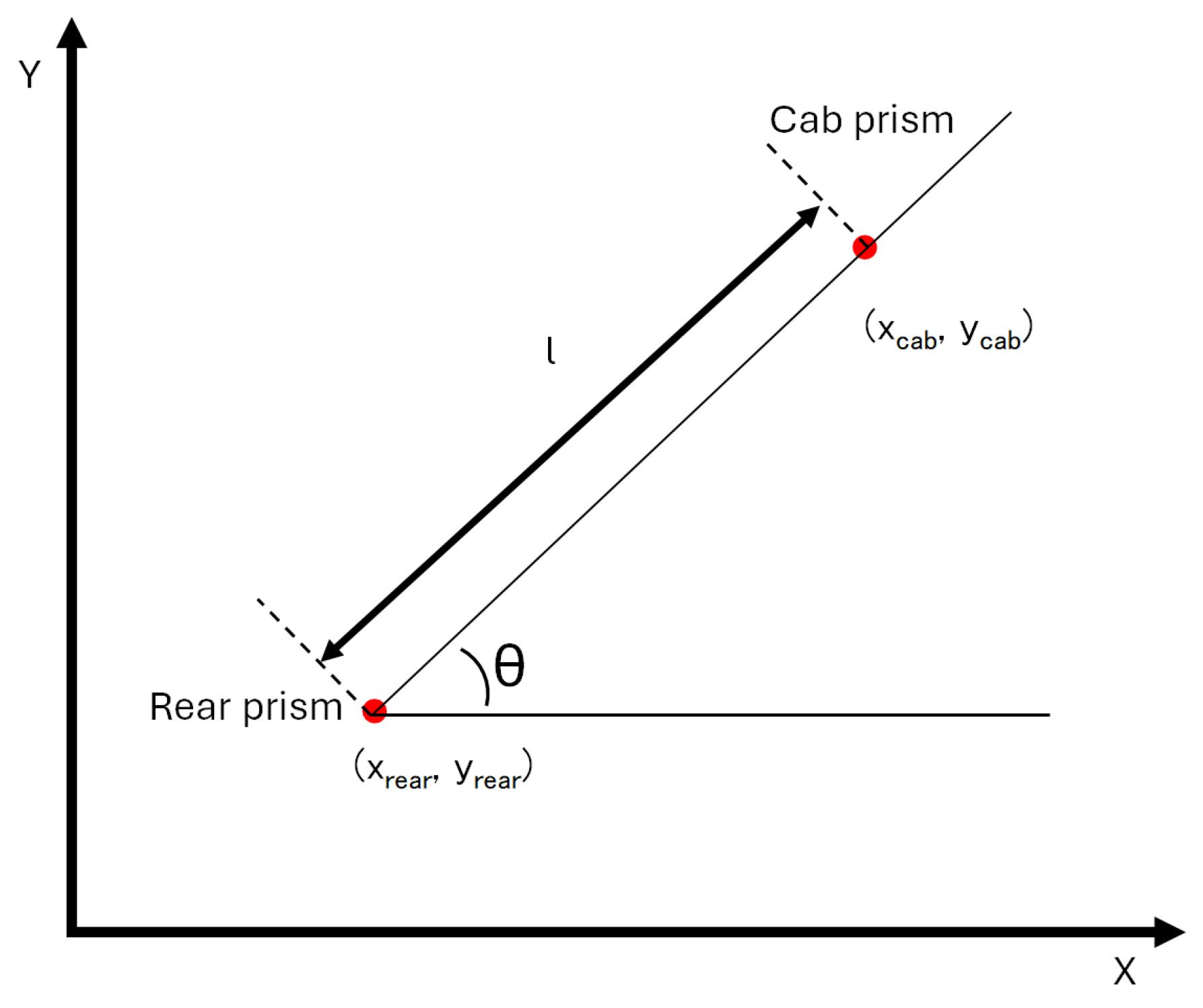
Estimation of Rear 3-Point Coordinates

The coordinates of the Rear 3-Point at a distance of L behind the agricultural tractor were calculated using Equation (21). These coordinates are based on the center coordinates $\left(x_k{,y}_k\right)$ of the tractor obtained through the EKF and the yaw angle ${\psi }_k$.

$$x_k^{rear}=x_k-Lcos\left({\psi }_k\right),\hspace{1em}{y}_k^{rear}=y_k-Lsin\left({\psi }_k\right)$$

(21)

2.5.5. Encoder-Only Attention Mechanism

The transformer architecture has the capacity to learn global dependencies across entire sequences without recursive sequential operations [20]. This architecture exhibits outstanding performance in terms of computational parallelism and learning speed. The structure of this study can be interpreted in a manner consistent with the encoder–decoder-based attention architecture utilized in translation models. A-KIT (adaptive Kalman-informed transformer), which employs an attention-based set transformer structure to estimate the process noise covariance matrix (Q) of an EKF in an adaptive manner, was proposed in 2025 [21]. The present study is fundamentally distinct from A-KIT with regard to both the application method and the objectives pursued. The primary distinction is that the present study focuses on high-precision disturbance suppression regression based on the cab location coordinates. The input sequence encompasses past cab location and yaw information, which is then summarized into patterns across the entire time series through the utilization of a transformer encoder. As illustrated in Figure 7, the AI learning flow of this study incorporates a time series of cab coordinates and yaw changes, derived from a sliding window, which are input into a transformer encoder-only structure. This structure is utilized to predict Rear 3-Point coordinates through the implementation of a regression method. Each input at each time point undergoes high-dimensional embedding, which reflects inter-temporal correlations through the multi-head self-attention mechanism. This is followed by a feed-forward network to enhance nonlinear expressiveness. The final encoder output (context vector) derived from this process is considered a state vector, which summarizes the entire time-series information. This state vector is then passed to a linear layer to predict the final coordinates. In the absence of a decoder or sequence output structure, this model, composed exclusively of an encoder, provides a straightforward and efficient structure that is well suited to single regression output problems. It also establishes a learning structure that dynamically emphasizes temporal information, which is crucial for Rear 3-Point coordinate estimation using attention mechanisms. Consequently, this configuration attains a resilient Rear 3-Point coordinate estimation performance, demonstrating immunity to non-stationary disturbances and temporal irregularities.

Input Configuration and Preprocessing

The transformer model of artificial intelligence utilized in this study initially passes the input sequence through an embedding layer. The length of the input sequence is 21, and the input vector at each point is composed of six dimensions, including $x_{cab}$, $y_{cab}$, $Sin\left(\theta \right)$, Cos$\left(\theta \right)$, $d_x$, and $d_y$, as shown in Equation (22).

$$X=[x\_1, x\_2, x\_3···,x\_t ],x\_t\in R^6$$

(22)

where $x_{cab},y_{cab}$ are $the cab coordinates$, $\theta$ is the $yaw of \mathrm{t}\mathrm{h}\mathrm{e} radian,$ and $d_x,d_y$ are the predicted displacements of the Rear 3-Point system.

Input Embedding Layer

As shown in Equation (23), each input point is converted into an $d_{model}=64$ dimensional embedding vector through a linear transformation. The final embedded input sequence is of size $R^{21\times 64}$.

$$E_t=W_{emb}{x}_t+b_{emb},E_t\in R^{64}$$

(23)

where $W_{embed}\in R^{64\times 6}$ and $b_{embed}\in R^{64\times 6}$ are trainable parameters. The sequence of embeddings $\left\{e_{t_0},e_{t_1},···,e_{t_{21}}\right\}$ is then fed into the encoder network.

Multi-Head Self-Attention Encoder

In this study, a multi-head self-attention (MHSA) structure was adopted, which implements multiple attention ‘heads’ in parallel. Each head learns different projection matrices (query, key, value) for the input sequence in order to identify correlations from various perspectives. The transformer encoder has been shown to effectively learn the semantic relationships and dependencies between each time point in the time-series data by applying the MHSA, as demonstrated in Equation (24). This mechanism learns the embeddings of each time point in the form of weights that represent the associations between the embeddings of different time points within the sequence.

$$Attention(Q, K, V)=softmax\left({\displaystyle \frac{Q_i{K}_i^T}{\sqrt{d_k}}}\right)V_i,i=1, ···, 4$$

(24)

The projection matrices for query, key, and value are defined in Equation (25).

$$Q_i=E·W_i^Q,K_i=E·W_i^K,V_i=E·W_i^V,d_k=16$$

(25)

where $Q,K,\mathrm{a}\mathrm{n}\mathrm{d}V$ are the query, key, and value, respectively; $E$ is the input embedding array; $W_i^q,W_i^q,{\mathrm{a}\mathrm{n}\mathrm{d} W}_i^q\in R^{64\times 16}$ are the projection matrices; and $d_k=16$ is the head dimension of the head.

The final attention output is generated by adjusting the output results of multiple heads into a single, consistent 64-dimensional representation within the model, as shown in Equation (26). This process prevents overfitting and the unnecessary diffusion of information.

$$Z=Concat({head}_1, {head}_2{head}_3,{head}_4)\times W^o$$

(26)

where ${\mathrm{W}}^{\mathrm{o}}\in {\mathrm{R}}^{64\times 64}$ is the output projection matrix.

It is imperative to direct attention to the residual connection between output Z and input E, as illustrated in Equation (27). Subsequently, layer normalization is applied.

$$Output=LayerNorm(Z+E)$$

(27)

where $Z$ is the attention output, and E is the input-embedding output.

Feedforward Neural Network (FFN)

The output of each time step, which has undergone a multi-head self-attention process, is processed through an FFN that is applied independently for each position to enhance the model’s nonlinear representation ability. The FFN under consideration consists of two fully connected layers, as illustrated in Equations (28) and (29), and performs the same operation for each time step. The calculation process is outlined as follows.

First hidden layer:

$$h_1=ReLu(z\times W_1+b_1),W_1\in R^{64\times 128},{ b}_1\in R^{128}$$

(28)

Second hidden layer:

$$h_2=ReLu(z\times W_2+b_2),W_1\in R^{128\times 64},{ b}_1\in R^{64}$$

(29)

where $z$ is the input vector from the previous add and norm layers (dimension 64), $W_1$ and $W_2$ are the weight matrices for the hidden and output layers, $b_1$ and $b_2$ are bias vectors, and $ReLu$ denotes the rectified linear unit activation function applied after the first linear transformation.

Final Output Projection and Loss Function

The expression vector obtained from the final hidden layer of the FFN is predicted through a linear transformation of Equation (30) using the two-dimensional coordinates of the Rear 3-Points. The model was trained in a direction that minimizes the mean squared error (MSE) between the predicted coordinates of Equation (31) and the actual answer coordinates based on EKF.

$$\widehat{y}=h_2\times W_3\times b_3,W_3\in R^{64\times 2}$$

(30)

$$L(\widehat{y},y)={\displaystyle \frac{1}{N}}\sum _{i=1}^N{‖{\widehat{y}}_i-y_i‖}^2$$

(31)

where $h_2$ is the second hidden layer, $W_3$ is the weight matrices for the hidden and output layers, $b_3$ is the bias vector, and $\widehat{y}$ is the predicted Rear 3-Point coordinate $\left[\widehat{x},\widehat{y}\right]$.

3. Results and Discussion

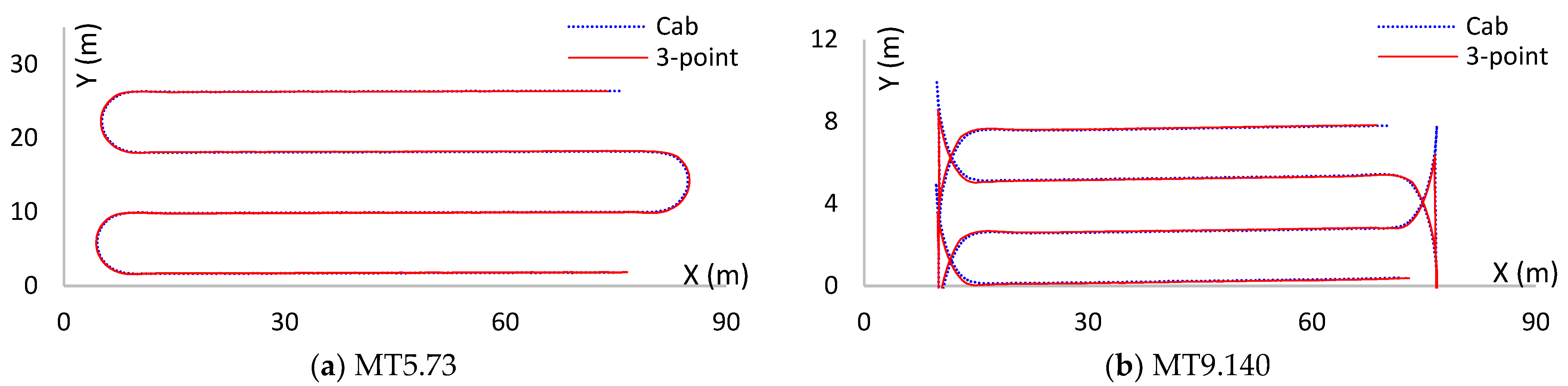
3.1. Experimental Measurement Results of Autonomous Driving Trajectories

In this study, the autonomous agricultural tractor trajectories that were utilized as fundamental data were obtained from two distinct models of agricultural tractors. The driving speed was recorded at 0.3 m/s, and trajectory data was measured at 10 Hz intervals using a total station. However, a loss of data was experienced, resulting in an actual collection cycle of approximately 8 Hz on average. The capture points and three support points were measured simultaneously, and during this process, minor temporal discrepancies of 10 Hz or less were observed. The results obtained from the autonomous agricultural tractor’s operation along the pre-planned autonomous driving path are presented in Figure 8.

The turning sections were excluded from the evaluation of autonomous path-following capability, as they were sections where the agricultural tractor did not perform actual agricultural work. Therefore, the data from the turning sections were excluded from this study.

The driving results were evaluated based on the difference between the planned and actual routes. This evaluation was conducted in accordance with the autonomous driving system test method of the Korea Agriculture Technology Promotion Agency. The following path error calculations were performed: 95th percentile cumulative error (95% CE), 50th percentile cumulative error (50% CE), standard deviation (SD), mean error (ME), and maximum error (MaxE). The results are shown in

Table 4. Evaluation results of trajectory errors based on 95% CE, 50% CE, SD, ME, and MaxE of autonomous tractors.

	1st (0 h)		2nd (+5 h)		3rd (+25 h)
Parameters	(a)	(d)	(a)	(d)	(a)	(d)
95% CE (mm)	32.9	30.7	52.3	23.0	35.5	13.5
50% CE (mm)	21.3	19.9	44.4	16.2	27.5	6.3
MaxE (mm)	39.5	39.0	63.2	28.0	42.4	18.0
ME (mm)	21.3	20.0	43.8	16.1	27.6	6.7
SD (mm)	6.6	5.9	5.4	4.3	4.8	4.0

.

3.2. Experimental Results on Installation Error Deviations of the Rear 3-Point Sensor

Furthermore, observations made according to the standard testing procedure of the Korea Agriculture Technology Promotion Agency (KOAT), which involves direct measurement of the Rear 3-Point, revealed that its installation position at the rear of the agricultural tractor tended to induce deviations from the intended driving trajectory. The root cause of this phenomenon was ascertained to be the installation and fixation conditions of the equipment, with the influence of the Rear 3-Point installation being partially reflected in the path error measurement results. The lateral deviation caused by Rear 3-Point was observed in the C-turn pattern of agricultural work during round-trip driving, as shown in Figure 9. Specifically, the driving paths of the first and third runs, and the second and fourth runs, exhibited deviations of approximately 10 cm.

Accordingly, additional tests were conducted to attach observation sensors to the Rear 3-Point system, and tests were performed to install sensors and jigs on an agricultural tractor in a stationary state. The results of the study are presented in

Table 5. Mean values and standard deviations for each installation.

Installation Position	Grouped Mean (3 Repeats × 4 Sets)				Total Mean (mm)	Std. Dev. (mm)
	Trial 1 (mm)	Trial 2 (mm)	Trial 3 (mm)	Trial 4 (mm)
Cab	145	146	146	145	145	0.6
Rear 3-Point	170	158	163	129	155	18.0

. If sensor position errors and measurement biases are not corrected simultaneously, the overall position estimation accuracy of the system can be significantly degraded, as demonstrated theoretically and through simulations [22]. In this study, it is posited that tilting the Rear 3-Point support system to one side during installation may result in the overlapping or missing of work areas during actual agricultural operations. Furthermore, during the process of autonomous driving precision evaluation, the initial sensor position selection may result in a lower precision evaluation in comparison to the actual autonomous driving performance of the agricultural tractor.

In this study, correlation analysis between installation error and trajectory error was considered. However, due to limitations in the experimental data, this analysis was not included in the final paper.

This issue will be addressed in future experiments. As shown in Figure 10, the predicted coordinates of the cab were estimated based on the EKF and the predicted coordinates of the Rear 3-Point. The cab sensor data, Rear 3-Point sensor values, and the trajectory of the Rear 3-Point, corrected using the Kalman filter, were then compared collectively. In the context of cab prediction, the yaw value was utilized to estimate the Rear 3-Point, which was located a specific distance l behind the center of the agricultural tractor. This estimation was achieved by removing noise using SKF.

Table 6. Euclidean distance-based analysis of cab and Rear 3-Point estimation performance.

Comparison (Measurement vs. EKF Results)			MAE (mm)	RMSE (mm)	Max Error (mm)	STD (mm)
MT5.73	Cab	Trial 1	0.0039	0.0037	0.0425	0.0046
		Trial 2	0.0035	0.0034	0.0254	0.0044
		Trial 3	0.0046	0.0044	0.0330	0.0055
	Rear 3-Point	Trial 1	49	42	276	50
		Trial 2	39	35	325	45
		Trial 3	47	42	305	52
MT9.140	Cab	Trial 1	0.0047	0.0037	0.0216	0.0039
		Trial 2	0.0045	0.0037	0.0276	0.0040
		Trial 3	0.0038	0.0034	0.0282	0.0041
	Rear 3-Point	Trial 1	195	122	411	65
		Trial 2	209	131	462	68
		Trial 3	188	133	422	111

presents the results of a quantitative analysis of the accuracy of predictions for the cab position and Rear 3-Point based on the Euclidean distance. Each item was compared in three repeated experiments using the mean absolute error (MAE), root mean square error (RMSE), maximum error (Max Error), and standard deviation (STD) to analyze the error characteristics. For cab position prediction, the average MAE was as low as 0.0047 mm, indicating a high level of agreement with actual cab position values. This is because the EKF-based estimation calculates the path based on measured cab position values. The RMSE and STD also remained low overall, supporting the reliability of cab path prediction. Conversely, for the Rear 3-Point, the average MAE was found to range from 49 to 209 mm, with a maximum error of 462 mm. This is attributed to the kinematic-based estimation model requiring the yaw value during Rear 3-Point estimation. However, the yaw value depends on the EKF-based predicted value rather than the actual measured value, leading to a slight decrease in accuracy. This is a major factor in errors in predicting Rear 3-Point position. Additionally, the EKF-based Rear 3-Point estimation method is considered to perform ‘ideal estimation’ based on a physics-based model. However, the actual measured Rear 3-Point position values included external factors, such as sensor installation errors, tire condition, engine vibration, uneven road surfaces, and wind. Therefore, the errors observed in this experiment are considered to be caused by these complex factors. In a previous experiment (Section 3.2), it was confirmed that left–right asymmetry in Rear 3-Point position installation significantly affected the driving path of an agricultural tractor and can result in overlap or omission of the work area during actual agricultural operations. This indicates that sensor installation deviations are not merely hardware errors, but rather factors that can distort the results of autonomous driving precision measurements. While the EKF’s prediction accuracy may appear lower in this context, the measured values themselves cannot be considered ‘true values’ due to uncertainties such as vibration, drift, and sensor installation errors. The EKF is an algorithm that theoretically performs ideal estimation under constant input conditions. It was also reported that, even under static conditions, the measured GNSS altitude values showed an average error of 6.34 m. It was only after applying the EKF and correction algorithms that a precision of 0.063 m was achieved [7]. Therefore, while the EKF-based Rear 3-Point prediction values in this study may differ from the measured values, it is difficult to attribute these differences solely to the prediction system.

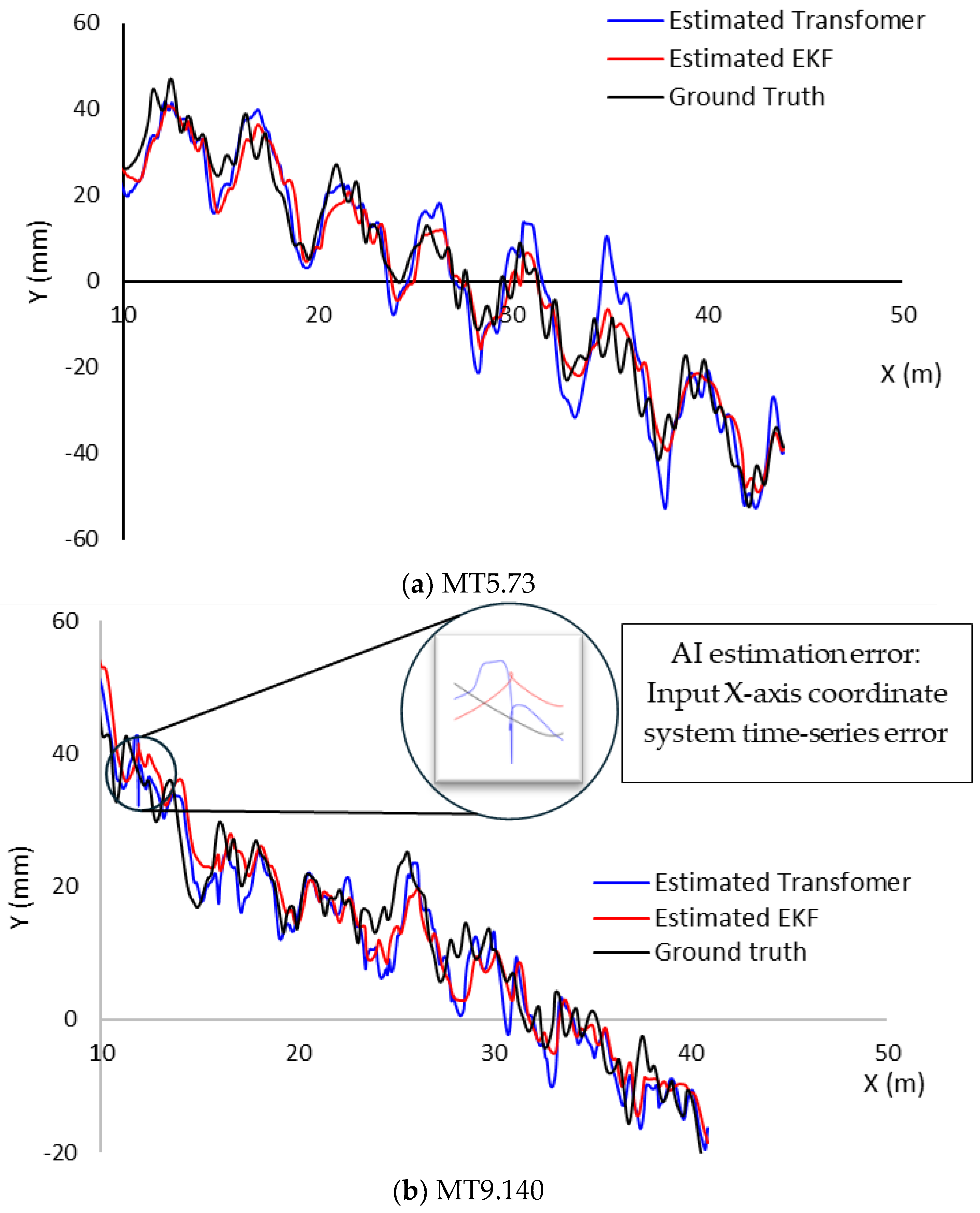
3.3. Comparison of Prediction Accuracy Between EKF Model and AI Model

The results of estimating the position of Rear 3-Point using an AI-based prediction model are presented in Figure 11. When evaluated in comparison with the cab sensor and the actual Rear 3-Point ground truth, the AI prediction generally exhibited a trajectory that was analogous, though cases of instability or sudden errors were observed in the initial section. In this study, input sequences for the AI prediction model were generated using a fixed-length sliding window of 100 time steps. Such sliding window structures are known to cause edge effects, where prediction accuracy is reduced at the beginning of the time series due to the lack of historical context [23]. The predicted trajectories were found to be relatively stable and exhibited a comparable flow to the actual measured paths, thereby confirming the learning and generalization capabilities of the AI model. This finding aligns with the results obtained using the TA-AEKF (transformer-aided adaptive extended Kalman filter) method [24]. Their research indicated that the combination of filter-based models surpassed the efficacy of utilizing a solitary AI model in ensuring the stability of time series.

The results of analyzing the Y-axis error, which is used as a measure of precision for autonomous agricultural tractors, are shown in

Table 7. Results of analyzed the Y-axis error of autonomous agricultural tractors.

Comparison (Predicted vs. Measured)		MAE (mm)	RMSE (mm)	Max Error (mm)	STD (mm)	R2
(a)	Measure vs. EKF	2.6	1.6	12.6	3.9	0.97
	Measure vs. AI	3.5	1.9	24.1	5.4	0.94
	EKF vs. AI	2.6	1.6	17.3	4.1	0.97
(b)	Measure vs. EKF	1.9	1.4	10.1	3.0	0.96
	Measure vs. AI	2.0	1.4	10.4	2.9	0.96
	EKF vs. AI	1.6	1.2	9.4	2.2	0.98

. This phenomenon can be attributed to the fact that the direction of travel for agricultural tractors is typically maintained with a high degree of consistency relative to the X-axis. In contrast, deviations in driving behaviors are more evident in the Y-axis (amplitude). Consequently, when evaluating the prediction performance of the AI model, a comparison of the predicted Y-axis values of Rear 3-Point with the original Y-coordinates of the cab is appropriate for evaluation purposes and effective for analyzing actual path-following precision. For the estimation of the EKF, the values were 0.97 and 0.96 for MT5.73 and MT9.140, respectively, with Rear 3-Point. The AI model demonstrated a high linear correlation between measured and predicted values at 0.94 and 0.96. For MT5.73, the maximum error recorded was 12.6 mm for the EKF and 24.1 mm for AI, suggesting that the EKF estimation model exhibited superior performance. This is likely attributable to the limited availability of training data, which has resulted in estimation errors in specific sections.

4. Conclusions

In this study, we sought to address the external disturbance problem that occurs during the measurement of the existing Rear 3-Point system. This study was conducted with the objective of analyzing the driving accuracy of autonomous agricultural tractors. Following the modification of the measurement points to the cab location, where external disturbances are comparatively minimal, a methodology was put forward for the indirect estimation of the trajectories of the Rear 3-Point system, which necessitate actual measurement, utilizing EKF and AI techniques. In addition, a statistical correlation between sensor installation error and trajectory deviation was analyzed in this study. As shown in Section 3.2 and Table 5, significantly larger deviations were observed when the sensor was installed at the Rear 3-Point (mean: 155 mm; standard deviation: 18.0 mm), compared to the cab installation (mean: 145 mm; standard deviation: 0.6 mm). These findings suggest that trajectory estimation accuracy can be critically affected by improper sensor alignment or tilting. Therefore, it is considered effective to use measurement data obtained from positions with minimal installation errors such as the cab to indirectly estimate the Rear 3-Point trajectory. Through this approach, bias caused by sensor installation can be minimized, thereby allowing for a more reliable and accurate assessment of driving trajectories. The experimental results demonstrate that the EKF-based prediction attained a maximum RMSE of 1.6 mm, a maximum error of 12.6 mm, and a maximum standard deviation of 3.9 mm in comparison to the actual measured values. The AI-based estimation also achieved a maximum root mean square error (RMSE) of 1.9 mm, a maximum error of 24.1 mm, and a maximum standard deviation of 5.4 mm, with both methods achieving prediction accuracy within 3.5 mm. This is a notable achievement, as it was accomplished utilizing solely cab coordinates, without the incorporation of supplementary sensors, such as IMU and steering sensors. The limitations of this study are twofold. Firstly, the removal of disturbances from the measured coordinates was not complete. Therefore, it is necessary to carry out additional verification under various disturbance conditions in the future. Nevertheless, the present study concentrated on the capacity of the attention mechanism to learn nonlinear patterns within time series and applied it to autonomous tractor path prediction, effectively suppressing complex external disturbance factors, such as vibration, skew, and sensor installation errors that occur during the measurement stage. In particular, the attention-based prediction results show a high degree of similarity to the actual measured values, demonstrating not only its applicability to autonomous agricultural tractors but also its practical scalability to other types of autonomous agricultural machinery, such as autonomous rice transplanters and combine harvesters, which are subject to significant vibration and oscillation at the implement section. Secondly, the computational complexity of the proposed model, along with the requirement for real-time disturbance suppression during the prediction phase, presents practical limitations for direct integration into commercial agricultural tractors that are not equipped with dedicated processing hardware. Nevertheless, recent advancements in autonomous agricultural machinery, such as the incorporation of onboard GPU modules and the ability to offload computational tasks to remote data centers via wireless communication, indicate promising potential for the practical deployment of the proposed approach in future agricultural systems.

References

1. Kim, Y.-T.; Kim, Y.-H.; Baek, S.-M.; Kim, Y.-J. Technology Trend on Autonomous Agricultural Machinery. J. Drive Control 2022, 95, 95–99. [Google Scholar]
2. Yuan, J.; Ji, W.; Feng, Q. Robots and Autonomous Machines for Sustainable Agriculture Production. Agriculture 2023, 13, 1340. [Google Scholar] [CrossRef]
3. Erenstein, O.; Chamberlin, J.; Sonder, K. Farms worldwide: 2020 and 2030 outlook. Outlook Agric. 2021, 50, 221–229. [Google Scholar] [CrossRef]
4. Qu, J.; Zhang, Z.; Qin, Z.; Guo, K.; Li, D. Applications of Autonomous Navigation Technologies for Unmanned Agricultural Tractors: A Review. Machines 2024, 12, 218. [Google Scholar] [CrossRef]
5. Han, J.-H.; Park, C.-H.; Jang, Y.Y.; Gu, J.D.; Kim, C.Y. Performance Evaluation of an Autonomously Driven Agricultural Vehicle in an Orchard Environment. Sensors 2022, 22, 114. [Google Scholar] [CrossRef]
6. Ren, H.; Wu, J.; Lin, T.; Yao, Y.; Liu, C. Research on an Intelligent Agricultural Machinery Unmanned Driving System. Agriculture 2023, 13, 1907. [Google Scholar] [CrossRef]
7. Xie, K.; Zhang, Z.; Zhu, S. Enhanced Agricultural Vehicle Positioning through Ultra-Wideband-Assisted Global Navigation Satellite Systems and Bayesian Integration Techniques. Agriculture 2024, 14, 1396. [Google Scholar] [CrossRef]
8. MAFRA Notification, No.2023-1; Standards for the Testing of Agricultural Machinery. Ministry of Agriculture, Food and Rural Affairs: Sejong, Repubic of Korea, 2023.
9. Korea Agriculture Technology Promotion Agency. Detailed implementation guidelines for testing and safety management of agricultural machinery. KOAT 2025. Available online: https://lab.koat.or.kr/front/analysis/AgriMachStruRsearchMethodAction.do?method=list&bbId=10 (accessed on 2 July 2025).
10. Antoshchenkov, R.; Antoshchenkova, V.; Kis, V.; Smitskov, D. Increasing accuracy of measuring functioning parameters of agricultural units. Eng. Rural Dev. 2023, 22, 210–215. [Google Scholar] [CrossRef]
11. Benterki, A.; Boukhnifer, M.; Judalet, V.; Maaoui, C. Artificial intelligence for vehicle behavior anticipation: Hybrid approach based on maneuver classification and trajectory prediction. IEEE Access 2020, 8, 56992–57002. [Google Scholar] [CrossRef]
12. Zhou, H.; Zhang, S.; Peng, J.; Zhang, S.; Li, J.; Xiong, H.; Zhang, W. Informer: Beyond Efficient Transformer for Long Sequence Time-Series Forecasting. Proc. AAAI 2021, 35, 11106–11115. [Google Scholar] [CrossRef]
13. Wen, Q.; Zhou, T.; Zhang, C.; Chen, W.; Ma, Z.; Yan, Z.; Yan, J.; Sun, L. Transformers in Time Series: A Survey. In Proceedings of the Thirty-Second International Joint Conference on Artificial Intelligence, Macao, China, 19–25 August 2023; Volume 23, pp. 6778–6786. [Google Scholar] [CrossRef]
14. Gan-Mor, S.; Clark, R.L.; Upchurch, B.L. Implement lateral position accuracy under RTK-GPS tractor guidance. Comput. Electron. Agric. 2007, 59, 31–38. [Google Scholar] [CrossRef]
15. Lim, R.-G.; Kim, T.-B.; Kim, W.-S.; Baek, S.-Y.; Jeon, H.-H.; Ham, J.-Y.; Yoo, C.; Kim, Y.-J. Development and validation of prediction model for exhaust emissions during tractor plow tillage. Agriculture 2024, 14, 2334. [Google Scholar] [CrossRef]
16. ISO 12188-1:2012; Tractors and Machinery for Agriculture and Forestry—Test Procedures for Positioning and Guidance Systems—Part 1: General Principles. International Organization for Standardization: Geneva, Switzerland, 2012.
17. ISO 12188-2:2012; International Organization for Standardization. Tractors and Machinery for Agriculture and Forestry—Test Procedures for Positioning and Guidance Systems—Part 2: Testing of Satellite-Based Auto-Guidance Systems During Straight and Level Travel. International Organization for Standardization: Geneva, Switzerland, 2012.
18. Hegedüs, F.; Bécsi, T.; Aradi, S.; Szalay, Z.; Gáspár, P. Real-time optimal motion planning for automated road vehicles. IFAC-Pap. 2020, 53, 15647–15652. [Google Scholar] [CrossRef]
19. Shen, S.; Chen, J.; Yu, G.; Zhai, Z.; Han, P. KalmanFormer: Using transformer to model the Kalman Gain in Kalman Filters. Front. Neurorobot. 2025, 18, 1460255. [Google Scholar] [CrossRef]
20. Vaswani, A.; Shazeer, N.; Parmar, N.; Uszkoreit, J.; Jones, L.; Gomez, A.N.; Kaiser, Ł.; Polosukhin, I. Attention is all you need. arXiv 2017. [Google Scholar] [CrossRef]
21. Cohen, N.; Klein, I. Adaptive Kalman-Informed Transformer. Eng. Appl. Artif. Intell. 2025, 146, 110221. [Google Scholar] [CrossRef]
22. Jia, T.; Liu, H.; Wang, P.; Wang, R.; Gao, C. Sensor Error Calibration and Optimal Geometry Analysis of Calibrators. Signal Process. 2024, 214, 109249. [Google Scholar] [CrossRef]
23. Willette, J.; Lee, H.; Lee, Y.; Jeon, M.; Hwang, S.J. Training-Free Exponential Extension of Sliding Window Context with Cascading KV Cache. arXiv 2024, arXiv:2406.17808. [Google Scholar] [CrossRef]
24. Zhang, H.; Yang, Z.; Xiong, H.; Zhu, T.; Long, Z.; Wu, W. Transformer aided adaptive extended Kalman filter for autonomous vehicle mass estimation. Processes 2023, 11, 887. [Google Scholar] [CrossRef]
25. Agricultural Machinery Information Platform. Official Data Verification Platform for Agricultural Machinery. rom. Available online: https://aminfo.or.kr/ (accessed on 2 July 2025).
Figure 1. Procedure for model development based on an autonomous agricultural tractor’s trajectory.
Agriculture 15 01475 g001
Figure 2. Autonomous agricultural tractors.
Agriculture 15 01475 g002
Figure 3. Total station and 360-degree prism.
Agriculture 15 01475 g003
Figure 4. Mounted prisms at the cab and rear 3-point positions.
Agriculture 15 01475 g004
Figure 5. Testing field, ground condition, and autonomous driving planned trajectory.
Agriculture 15 01475 g005
Figure 6. Kinematic model of autonomous agriculture tractor.
Agriculture 15 01475 g006
Figure 7. Encoder-only transformer model for Rear 3-Point coordinate prediction.
Agriculture 15 01475 g007
Figure 8. Trajectory measurement results of autonomous tractors under identical test conditions: (a) MT5.73 tractor; (b) MT9.140 tractor.
Agriculture 15 01475 g008
Figure 9. Rear 3-Point trajectory deviation from sensor installation error.
Agriculture 15 01475 g009
Figure 10. EKF-based estimation of cab and Rear 3-Point with yaw Kalman filtering. (a) MT5.73 tractor; (b) MT9.140 tractor.
Agriculture 15 01475 g010
Figure 11. EKF-based estimation of cab and Rear 3-Point positions with yaw Kalman filtering. (a) MT5.73 tractor; (b) MT9.140 tractor.
Agriculture 15 01475 g011