Article

An Optimized Multi-Stage Framework for Soil Organic Carbon Estimation in Citrus Orchards Based on FTIR Spectroscopy and Hybrid Machine Learning Integration

1
Guangxi Academy of Agricultural Sciences, Nanning 530007, China
2
Guangxi Vocational & Technical Institute of Industry, Nanning 530001, China
*
Author to whom correspondence should be addressed.
Agriculture 2025, 15(13), 1417; https://doi.org/10.3390/agriculture15131417
Submission received: 8 May 2025 / Revised: 24 June 2025 / Accepted: 26 June 2025 / Published: 30 June 2025
(This article belongs to the Section Agricultural Technology)

Abstract

Soil organic carbon (SOC) is a critical indicator of soil health and carbon sequestration potential. Accurate, efficient, and scalable SOC estimation is essential for sustainable orchard management and climate-resilient agriculture. However, traditional visible–near-infrared (Vis–NIR) spectroscopy often suffers from limited chemical specificity and weak adaptability in heterogeneous soil environments. To overcome these limitations, this study develops a five-stage modeling framework that systematically integrates Fourier Transform Infrared (FTIR) spectroscopy with hybrid machine learning techniques for non-destructive SOC prediction in citrus orchard soils. The proposed framework includes (1) FTIR spectral acquisition; (2) a comparative evaluation of nine spectral preprocessing techniques; (3) dimensionality reduction via three representative feature selection algorithms, namely the Successive Projections Algorithm (SPA), Competitive Adaptive Reweighted Sampling (CARS), and Principal Component Analysis (PCA); (4) regression modeling using six machine learning algorithms, namely the Random Forest (RF), Support Vector Regression (SVR), Gray Wolf Optimized SVR (SVR-GWO), Partial Least Squares Regression (PLSR), Principal Component Regression (PCR), and the Back-propagation Neural Network (BPNN); and (5) comprehensive performance assessments and the identification of the optimal modeling pathway. The results showed that second-derivative (SD) preprocessing significantly enhanced the spectral signal-to-noise ratio. Among feature selection methods, the SPA reduced over 300 spectral bands to 10 informative wavelengths, enabling efficient modeling with minimal information loss. The SD + SPA + RF pipeline achieved the highest prediction performance (R2 = 0.84, RMSE = 4.67 g/kg, and RPD = 2.51), outperforming the PLSR and BPNN models. This study presents a reproducible and scalable FTIR-based modeling strategy for SOC estimation in orchard soils. Its adaptive preprocessing, effective variable selection, and ensemble learning integration offer a robust solution for real-time, cost-effective, and transferable carbon monitoring, advancing precision soil sensing in orchard ecosystems.

1. Introduction

Soil organic carbon (SOC) is one of the most essential carbon storage forms in terrestrial ecosystems, playing a crucial role in regulating climate and maintaining ecological balance. SOC directly influences greenhouse gas emissions through the processes of mineralization and decomposition, thereby impacting the progression of global climate change [1,2]. Through photosynthesis, plants convert atmospheric CO2 into organic compounds, which microorganisms further transform into soil organic matter, ultimately achieving carbon sequestration [3]. SOC is a complex organic compound formed by humifying plant residues and microbial metabolites. SOC is a key indicator for evaluating soil carbon storage and plays an irreplaceable role in maintaining soil fertility and regulating ecosystem functions [4]. The precise quantification of SOC has become a vital basis for soil health assessments, carbon sink evaluations, and precision agricultural decision-making. Moreover, enhancing SOC monitoring has become increasingly strategic for national carbon neutrality goals, orchard ecosystem sustainability, and the development of intelligent agricultural systems.
Citrus is one of China’s most widely cultivated, highest-yielding, and most consumed fruit crops, with a total planting area reaching 44.9372 million mu [5]. In tandem with the intensification of citrus production, the demand for precise orchard management has grown significantly. Rapid, accurate, and scalable SOC assessments are crucial for optimizing fertilization strategies and maintaining long-term soil productivity. However, conventional wet chemical techniques (e.g., potassium dichromate oxidation with external heating) remain constrained by low sampling density, high costs, and time-consuming workflows, thereby limiting their applicability in real-time decision-making contexts.
Fourier Transform Infrared spectroscopy (FTIR) has attracted considerable attention in agronomy in recent years due to its advantages of being non-destructive, fast, easy to operate, and environmentally friendly [6]. FTIR measures changes in the vibrational frequencies of functional groups in samples, revealing their organic composition and structural characteristics [7]. It has been widely applied in the early diagnosis of crop pests and diseases, monitoring nutrient stress responses, and quantitative analysis of organic components [8,9]. Studies have shown that under nutrient deficiency or disease stress conditions, crop organs undergo chemical composition changes that alter their FTIR spectral characteristics, indicating FTIR’s potential to detect variations in soil and plant organic components [10]. Compared to traditional hyperspectral or visible–near-infrared (Vis-NIR) techniques, FTIR in the mid-infrared range more accurately identifies functional groups such as C=O, C-H, and O-H in organic compounds. This sensitivity to different carbon components in SOC provides a theoretical advantage for its quantitative inversion [11]. However, current studies on FTIR’s application to orchard soils, especially in estimating SOC content in citrus orchards, remain limited, and its modeling methods, variable extraction strategies, and applicability under heterogeneous soil conditions require further exploration.
Existing research indicates that regression models play a significant role in SOC spectral inversion. Linear modeling methods, such as Principal Component Regression (PCR) [12], Multiple Stepwise Regression (MSR) [13], and Partial Least Squares Regression (PLSR) [14], can effectively predict SOC content to a certain extent. However, nonlinear relationships typically exist between SOC and spectral data, making nonlinear algorithms such as Random Forest (RF), Support Vector Machine Regression (SVMR), and Back-propagation Neural Networks (BPNNs) perform better in SOC prediction [15,16,17]. Nevertheless, most existing studies focus on single-step algorithmic optimization and lack an integrated approach that jointly addresses spectral preprocessing, variable selection, and model architecture, limiting the reproducibility, generalizability, and practical scalability of SOC inversion pipelines in heterogeneous soil environments.
In conclusion, Fourier Transform Infrared (FTIR) spectroscopy offers substantial promise for the rapid and non-destructive estimation of soil organic carbon (SOC) content in citrus orchards, particularly under spatially heterogeneous field conditions. To fully leverage the chemical specificity of FTIR and address the limitations of traditional modeling approaches, this study establishes a structured five-stage modeling framework designed to optimize prediction accuracy and generalizability across diverse soil environments. The proposed workflow consists of the following components: (1) Spectral Acquisition: Collection of mid-infrared FTIR spectra within the 400–4000 cm−1 range, capturing key vibrational signals associated with SOC-related functional groups; (2) Preprocessing Evaluation: Comparative analysis of nine widely adopted spectral preprocessing techniques to enhance signal clarity and spectral stability; (3) Feature Selection and Dimensionality Reduction: Application of three representative variable selection algorithms—the Successive Projections Algorithm (SPA), Competitive Adaptive Reweighted Sampling (CARS), and Principal Component Analysis (PCA)—to isolate informative spectral bands while minimizing redundancy in high-dimensional data; (4) regression modeling using six machine learning algorithms, namely the Random Forest (RF), Support Vector Regression (SVR), Gray Wolf Optimized SVR (SVR-GWO), Partial Least Squares Regression (PLSR), Principal Component Regression (PCR), and the Back-propagation Neural Network (BPNN); and (5) comprehensive performance assessments and the identification of the optimal modeling pathway. This study is guided by three core hypotheses: (1) Nonlinear models such as the Random Forest (RF) and Back-propagation Neural Networks (BPNNs) can better capture the nonlinear and spatially variable relationships between FTIR spectral features and SOC content. (2) Variable selection methods (SPA, CARS, and PCA) significantly improve modeling efficiency and accuracy by identifying chemically relevant spectral bands associated with organic carbon. (3) A unified modeling pipeline that integrates spectral preprocessing, feature selection, and model training provides synergistic benefits, improving robustness and predictive performance for SOC estimation in complex agroecosystems.

2. Materials and Methods

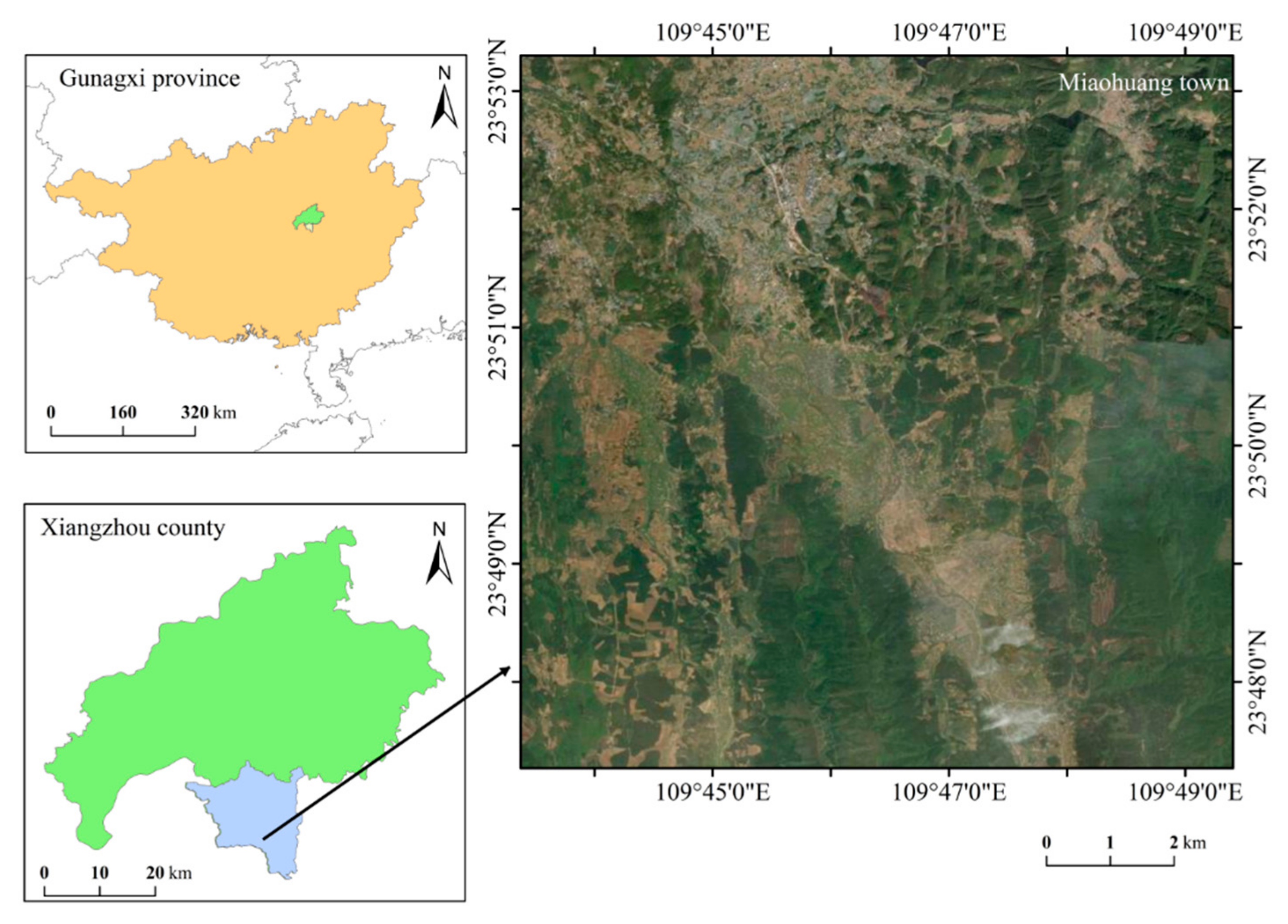
2.1. Overview of the Study Area

The study area is in Xiangzhou County, which is under the jurisdiction of Laibin City in Guangxi. It is situated in central Guangxi, on the western slope of the Dayao Mountains, between 109°25′ and 110°06′ east longitude and 23°44′ and 24°18′ north latitude (Figure 1). Xiangzhou County is located in the monsoon transition zone from the northern edge of the southern subtropics to the central subtropics, characterized by distinct monsoon features. Light, heat, and water are generally synchronized in the same season. With over 1700 h of annual sunshine, conditions favor citrus coloring. During the autumn and winter seasons, as citrus fruits enlarge and ripen, the significant day–night temperature differences promote the accumulation of organic matter and sugar conversion in citrus. Xiangzhou’s Shatang mandarins and other products have received national geographic indication agricultural product certification [18]. A total of 149 soil samples were collected from multiple citrus orchards within an approximately 10 km2 area in Miaohuang Township. The orchards were located in close proximity, with partially overlapping boundaries, and sampling points were evenly distributed at intervals of approximately 80 m. Due to the small size of the orchards and the limited spatial resolution of the background imagery, individual sampling points could not be clearly represented on the map. Nevertheless, all sampled orchards were managed under consistent agricultural practices, including seasonal pruning, biannual fertilization, and the absence of ground cover, thereby ensuring comparability among sites.

2.2. Soil Sample Collection

Soil samples were collected from Miaohuang Township, Xiangzhou County, Guangxi Zhuang Autonomous Region. Sampling was conducted in November 2024 using a grid-based method to ensure uniform coverage. Soil samples were collected from a depth of 0 to 60 cm, with approximately 80 m between sampling points, Each sampling point was located 30 cm inward from the edge of the citrus tree canopy projection, using a soil auger with a 7 cm diameter and a 20 cm drill length for collection. After mixing soil from different layers, the quartering method was used to discard excess materials, and approximately 0.5 kg of soil was retained for laboratory spectral and property measurements. The geographic coordinates of each sampling point were recorded in detail. The 149 collected soil samples were air-dried in the laboratory after removing debris, passed through a 2 mm sieve, and divided into two portions: One portion was used for the laboratory’s Fourier Transform Infrared (FTIR) spectroscopy analysis. The remaining portion of each soil sample was analyzed for soil organic carbon (SOC) content using an elemental analyzer (Vario EL III, Elementar Analysensysteme GmbH, Langenselbold, Germany). All soil samples were air-dried at room temperature (~25 °C) for seven days, ground with a mechanical grinder, and sieved through a 2 mm mesh. For FTIR analysis, a portion of each sample was further milled to pass through a 0.15 mm sieve to ensure uniform particle size and maximize spectral consistency.

2.3. Division of Calibration and Prediction Datasets

To construct hyperspectral inversion models for soil organic carbon (SOC) content under different sample set conditions, this study employed the Kennard–Stone (KS) algorithm to partition the dataset, ensuring that the modeling set is representative and captures the main spectral variability. This algorithm is based on the Euclidean distance between samples in the feature space, and it prioritizes the selection of the most widely distributed and representative samples for inclusion in the modeling set. The steps are as follows: First, we compute the Euclidean distances among all samples in the dataset and select the two samples with the most significant distance as the initial modeling samples. Subsequently, in each iteration, the sample with the maximum minimum Euclidean distance from the existing modeling samples is selected from the remaining dataset and added to the modeling set. This process is repeated until the desired number of modeling samples is reached, achieving uniform selection and ensuring representativeness. The Euclidean distance is calculated using the following formula:
d x p , q = j = 1 N [ x p j x q j ] 2 ,   p , q [ 1 , N ]
Here, xp and xq represent two different samples, and N denotes the number of spectral bands in the samples.

2.4. Soil Spectral Data Preprocessing

The infrared spectra of the soil samples were collected using the Diffuse Reflectance Infrared Fourier Transform (DRIFT) spectrometer (Nicolet iS5, Thermo Fisher Scientific Inc., Waltham, MA, USA) with a spectral range of 400–4000 cm−1 and a resolution of 4 cm−1. Each sample was scanned 32 times to enhance the stability of the spectral signals. The raw spectral data were preprocessed to minimize environmental noise interference, improve the signal-to-noise ratio (SNR), and enhance hyperspectral inversion models’ stability and generalization capability. In this study, nine commonly used and effective preprocessing methods were applied to the raw spectra using Python 3.7: the First Derivative (FD), the Second Derivative (SD), Multiplicative Scatter Correction (MSC), Standard Normal Variate (SNV), De-trending, Normalization, Zero-centering, Savitzky–Golay Smoothing (SG Smoothing), and Moving Average Smoothing. Each preprocessing method was applied separately and independently to the raw spectral dataset to ensure a fair comparative evaluation of its effect on model performance. No preprocessing methods were applied sequentially or in combination during the initial evaluation phase. These techniques help reduce baseline drift, scattering effects, and systematic errors, thereby enhancing the extraction of spectral features and providing more reliable input variables for subsequent modeling [19].

2.5. Feature Spectral Selection for Soil Organic Carbon Content

To improve the predictive accuracy and generalization capability of the model, three feature variable selection methods were employed to extract characteristic spectral information related to soil organic carbon (SOC) content: Competitive Adaptive Reweighted Sampling (CARS), the Successive Projections Algorithm (SPA), and Principal Component Analysis (PCA). These methods were applied to the preprocessed spectral data and the corresponding SOC content data for model construction. The CARS method iteratively updates weights to identify spectral features most strongly associated with the target variable from the full spectrum [20]. The SPA method selects highly representative and minimally redundant spectral bands by minimizing multicollinearity among variables [21]. The PCA method extracts principal components through linear dimensionality reduction to construct a principal component regression model, thereby reducing data dimensionality and mitigating noise interference [22]. All feature band selection procedures were conducted in the MATLAB 2012a environment, where feature compression and selection were performed based on the principles of each algorithm, providing essential variable support for subsequent hyperspectral inversion modeling.

2.6. Model Construction and Accuracy Validation

This study employed six representative machine learning methods to construct hyperspectral inversion models for soil organic carbon (SOC) content: Partial Least Squares Regression (PLSR), Support Vector Regression (SVR), the Random Forest (RF), Principal Component Regression (PCR), the Back-propagation Neural Network (BPNN), and Support Vector Regression optimized by the Gray Wolf Optimizer (SVR-GWO). Among these, the SVR-GWO model incorporated the Competitive Adaptive Reweighted Sampling (CARS) algorithm for spectral feature selection, further enhancing model performance. Model development and execution were conducted on different platforms: the PLSR, SVR, RF, PCR, and SVR-GWO models were implemented in the Python 3.7 environment, whereas the BPNN model was constructed and trained using MATLAB R2012a. To comprehensively evaluate the accuracy and robustness of each model in SOC prediction, three evaluation metrics were employed: the Coefficient of Determination (R2), Root Mean Square Error (RMSE), and Residual Prediction Deviation (RPD).
The formulas for these evaluation metrics are provided as follows [17,23,24]:
R 2 = 1 i = 1 n ( y ^ i y i ) 2 i = 1 n ( y i y - ) 2
R M S E = 1 n i = 1 n ( y ^ i y i ) 2
R P D = S D R M S E
where yi is the observed value, y ^ i is the predicted value, y - is the mean of the observed values, SD is the standard deviation of the observed values, and n is the number of samples.
Minor grammatical corrections were performed using Grammarly, an AI-based writing assistant, under full human oversight to ensure scientific accuracy.

3. Results

3.1. Descriptive Statistical Features of Soil Organic Carbon Content in Citrus Soil

According to the statistical results (Table 1), the soil organic carbon (SOC) content of the 149 collected citrus orchard soil samples ranged from 4.86 g/kg to 87.75 g/kg, with an average value of 24.91 g/kg and a coefficient of variation (CV) of 0.49, indicating moderate variability across the study area. The dataset was split using the Kennard–Stone (KS) algorithm into a calibration set (99 samples) and a validation set (50 samples). The calibration set retained a broad SOC range (5.38–87.75 g/kg), with a slightly higher mean (25.63 g/kg) and a similar CV (0.48), ensuring good representativeness for model training. The validation set exhibited a reduced upper SOC bound (max 49.29 g/kg), with a mean of 23.46 g/kg and a CV of 0.50, indicating consistent variability though with lower high-value coverage. This magnitude of variability (CV ≈ 0.48–0.50) is consistent with findings from similar subtropical soils in southern China, where grass-covered and citrus orchard soils exhibited moderate SOC fraction changes controlled by soil texture and age-related factors and where citrus orchard soil structure showed significant SOC differences under varied microtopography and erosion treatments [25]. Furthermore, studies in hilly red-soil regions of southern China reported CVs of 49.0–55.9% across 0–60 cm soil depths [26]. These parallels affirm the sampling representativeness and underscore the need for predictive models that can accommodate such moderate-to-high spatial heterogeneity.

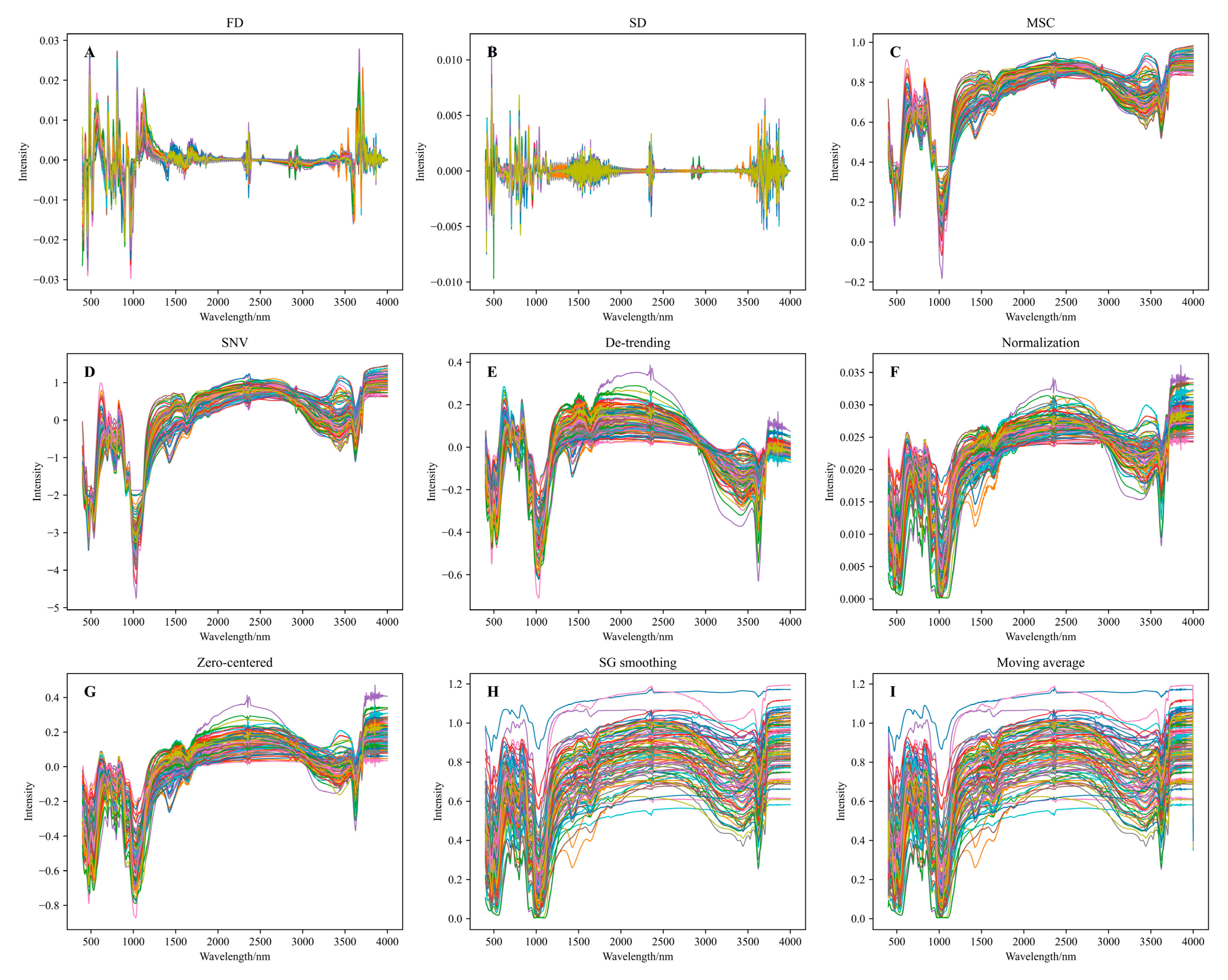
3.2. Soil Spectral Preprocessing and Method Selection for Citrus Soil

As shown in Figure 2, different spectral preprocessing methods significantly affected the shape and distribution characteristics of the soil spectral reflectance curves. Among them, the First-Derivative (FD) transformation compressed and smoothed the baseline drift of the original spectral curve, causing the fluctuation frequency of the processed curve to increase significantly, with multiple prominent peaks and valleys. The overall changes were concentrated near the X-axis, and the reflectance values included both positive and negative values, enhancing the expression of spectral detail features. On this basis, the Second-Derivative (SD) transformation further amplified the trends in the FD, making the spectral curve approximately symmetric with respect to the X-axis. The reflectance fluctuation at both ends of the curve became larger, highlighting subtle feature differences, but it may also introduce more high-frequency noise. Five methods, including Multiplicative Scatter Correction (MSC), Standard Normal Variate (SNV), Savitzky–Golay Smoothing (SG Smoothing), Normalization, and Moving Average Smoothing, effectively reduced spectral noise while retaining the overall trend of the original spectrum. Among them, the reflectance values after SG smoothing and Moving Average processing were positive, resulting in smoother curves. In contrast, the curves processed with the SNV, De-trending, Normalization, and Zero-centered methods exhibited positive and negative values, with the reflectance curves symmetrically distributed around the X-axis. In particular, De-trending and Zero-centered treatments enhanced the spectral reflectance differences between different samples, amplifying the feature contrasts among samples, which supports the model in capturing subtle variations between the data. In summary, different preprocessing methods have significantly different impacts on spectral shape. The appropriate preprocessing strategy should be selected based on the modeling requirements to retain valuable information while minimizing noise interference.
Different spectral preprocessing methods had significant effects on the inversion performance of the Partial Least Squares Regression (PLSR) model in predicting soil organic carbon (SOC) content in citrus soils (Table 2). The results indicated that the model built with spectral data preprocessed by the Second Derivative (SD) achieved the best performance, with an R2 of 0.886, an RMSE of 4.129, and an RPD of 2.973 on the calibration set, indicating high accuracy and stability in fitting. In contrast, the model based on First-Derivative (FD) preprocessing showed weaker performance, with an R2 of 0.770, an RMSE of 5.852, and an RPD of 2.098 on the calibration set, suggesting that although FD enhances spectral variability, it may also introduce substantial noise that hampers model fitting. Additionally, models built using the seven other preprocessing techniques—Multiplicative Scatter Correction (MSC), Standard Normal Variate (SNV), De-trending, Normalization, Zero-centering, Savitzky–Golay (SG) smoothing, and Moving Average—showed overall moderate performance in terms of accuracy and stability. Notably, the prediction results on the test set using SNV and Moving Average were relatively similar, with R2 values of 0.774 and 0.624, respectively, and no significant differences in RMSE and RPD values. It is worth mentioning that although the FD-based model performed better on the test set (R2 = 0.821, RMSE = 4.905, and RPD = 2.385) than on the calibration set, its overall stability was still inferior to the SD-based model. The SD-based model also exhibited good generalization ability on the test set, with an R2 of 0.765, an RMSE of 5.617, and an RPD of 2.082, confirming its robustness across different datasets. In conclusion, Second-Derivative (SD) preprocessing can significantly improve the predictive performance of the PLSR model for SOC. Based on the performance in both the calibration and test sets, the SD-based model can serve as a solid foundation for subsequent feature band selection and model optimization, potentially enhancing the accuracy and stability of SOC hyperspectral inversion.

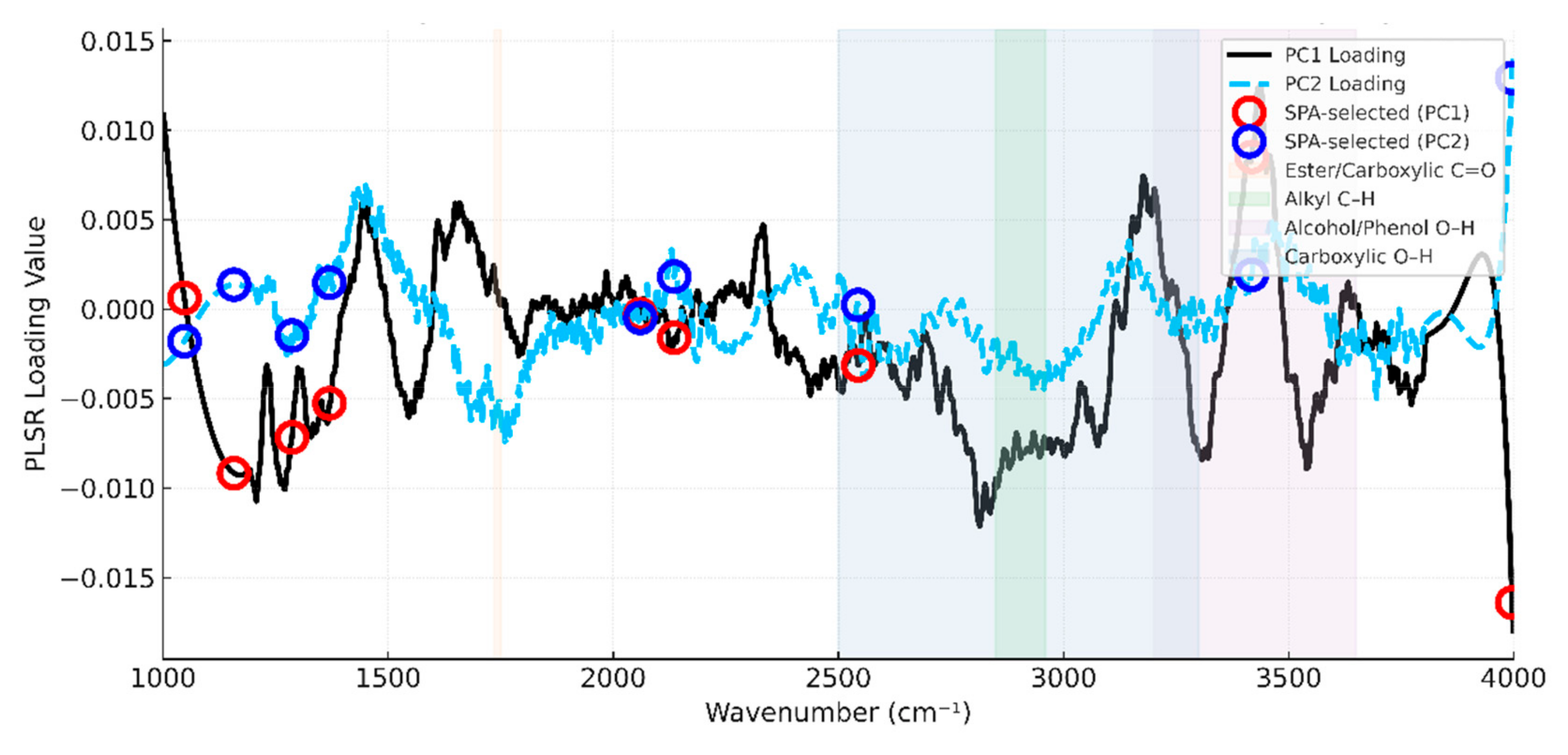
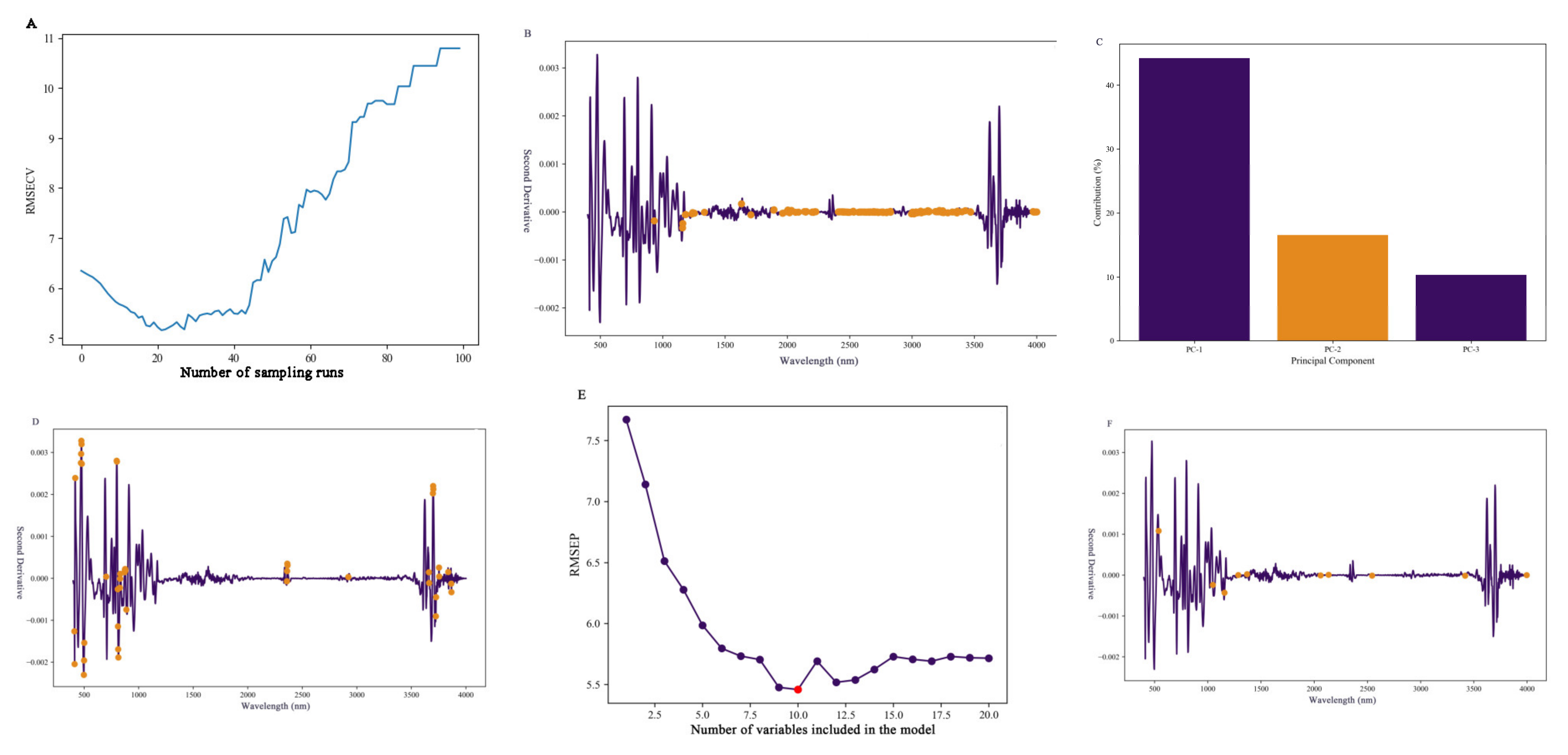
3.3. Selection of Spectral Feature Bands and Optimization of Methods for Citrus Soil

Figure 3 illustrates the operational procedures and selection outcomes of three spectral feature selection algorithms—CARS, PCA, and SPA—highlighting notable differences in their variable compression mechanisms and the number of selected features. In the Competitive Adaptive Reweighted Sampling (CARS) algorithm, the cross-validation Root Mean Square Error (RMSECV) exhibits a typical “decrease-then-increase” trend with the number of iterations (Figure 4A). In the initial phase (iterations 1–25), the RMSECV rapidly decreases, indicating that the selected variables gradually improve model fitting, reaching a minimum value of 5.155 g/kg at the 25th iteration. After that, the RMSECV enters a phase of slight fluctuation, rises markedly by the 50th iteration (6.318 g/kg), and increases sharply from the 51st iteration, eventually stabilizing at the maximum value (10.793 g/kg) at the 100th iteration. This indicates that variable redundancy rises as the number of iterations increases, weakening model performance. As shown in Figure 4B, when the RMSECV reaches its minimum, the CARS algorithm selects 152 practical spectral features. The dimensionality reduction results of the Principal Component Analysis (PCA) are shown in Figure 4C. The first principal component accounts for 44.19% of the variance. In comparison, the second and third components explain 16.56% and 10.35%, respectively, together explaining 71.7% of the total data variance, indicating that the first three principal components capture most of the vital information. The marginal contributions of subsequent components decrease significantly, and increasing the number of components further yields limited improvement in model performance. Figure 4D shows that 23 feature variables were identified based on the first three principal components. The Successive Projections Algorithm (SPA) shows a clear negative correlation between the number of selected spectral bands and the cross-validation error (Figure 4E). As the number of spectral features increases, the model’s RMSE generally decreases and reaches its lowest value (RMSEP = 5.46 g/kg) when ten variables are selected, indicating an optimal feature set. Figure 4F shows that the SPA ultimately selected 10 spectral features. In summary, CARS, PCA, and the SPA demonstrated different mechanisms and stabilities in spectral feature selection. CARS can identify spectral bands with strong relevance to the target variable within an ample variable space, though it tends to select more features. PCA compresses variables effectively through dimensionality reduction by extracting principal components but may miss some nonlinear information. The SPA excels at minimizing multicollinearity and selects the fewest variables, resulting in a more parsimonious model. These differences offer diverse input feature options for subsequent modeling.
To further investigate the influence of different spectral feature selection methods on the inversion accuracy of soil organic carbon (SOC) content, this study constructed Partial Least Squares Regression (PLSR) models using feature bands selected by three algorithms—CARS, PCA, and SPA—and evaluated their predictive performance on citrus soil samples. The comparative results of inversion accuracy among the models are presented in Figure 4.
As shown in Table 3, the Partial Least Squares Regression (PLSR) models constructed using the full spectrum and three feature selection methods (CARS, PCA, and SPA) were all capable of effectively predicting the soil organic carbon (SOC) content in citrus soils, with residual prediction deviation (RPD) values all greater than 1.50, indicating good predictive ability. Regarding the number of selected features, CARS, PCA, and SPA identified 152, 23, and 10 key spectral bands, significantly reducing the input dimensionality. Compared with full-spectrum modeling, this improved computational efficiency and reduced model complexity. The performance comparison on the calibration set showed that the model based on CARS had the best fitting results, with an R2 of 0.96, an RMSE of 3.36, and an RPD of 4.08, indicating excellent fitting capability on the training data. In contrast, PCA showed the weakest performance on the calibration set, with an R2 of only 0.78, an RMSE of 7.61, and an RPD of 1.61, suggesting that although PCA effectively compresses dimensions, it may omit some critical predictive information. The model constructed using SPA demonstrated intermediate performance, with an R2 of 0.81, an RMSE of 7.18, and an RPD of 1.70 on the calibration set, indicating moderate modeling capability. The differences in predictive performance on the test set were more pronounced. The CARS model achieved an R2 of 0.0.86, an RMSE of 6.12, and an RPD of 1.89 on the test set. Although it performed well in training, its generalization capability appeared slightly limited. The PCA model showed an R2 of only 0.66 on the test set, with the RMSE reaching 8.77 and the RPD dropping to 1.32, further confirming its limitations in extrapolation. In contrast, the SPA model demonstrated the best test set performance, with an R2 of 0.89, an RMSE of 5.46 g/kg, and an RPD of 2.12, achieving high predictive accuracy and strong stability and generalization capability. In summary, although the CARS model had the highest fitting accuracy on the calibration set, the SPA model achieved superior predictive performance and stability on the test set using only 10 key variables, demonstrating an excellent balance between feature compression and model performance. These results suggest that the SPA offers more significant application potential as an efficient and robust feature selection strategy in hyperspectral inversion soil organic carbon content modeling.
To further support the reliability of the SPA, we conducted a supplementary chemical interpretability analysis of the selected features. As detailed in Appendix A (Figure A1 and Figure A2 and Table A1), the SPA-selected wavenumbers were mainly located within key FTIR functional regions, especially those associated with C–O and O–H stretching vibrations—functional groups known to be indicative of organic matter. Furthermore, the PLSR loading profiles confirmed that these selected bands corresponded to regions of high model influence. This dual confirmation from the chemical and statistical perspectives reinforces the applicability and interpretability of SPA in modeling SOC content.

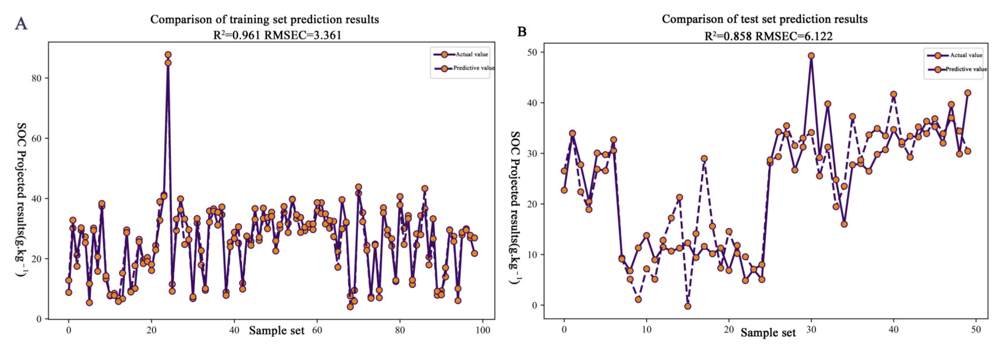
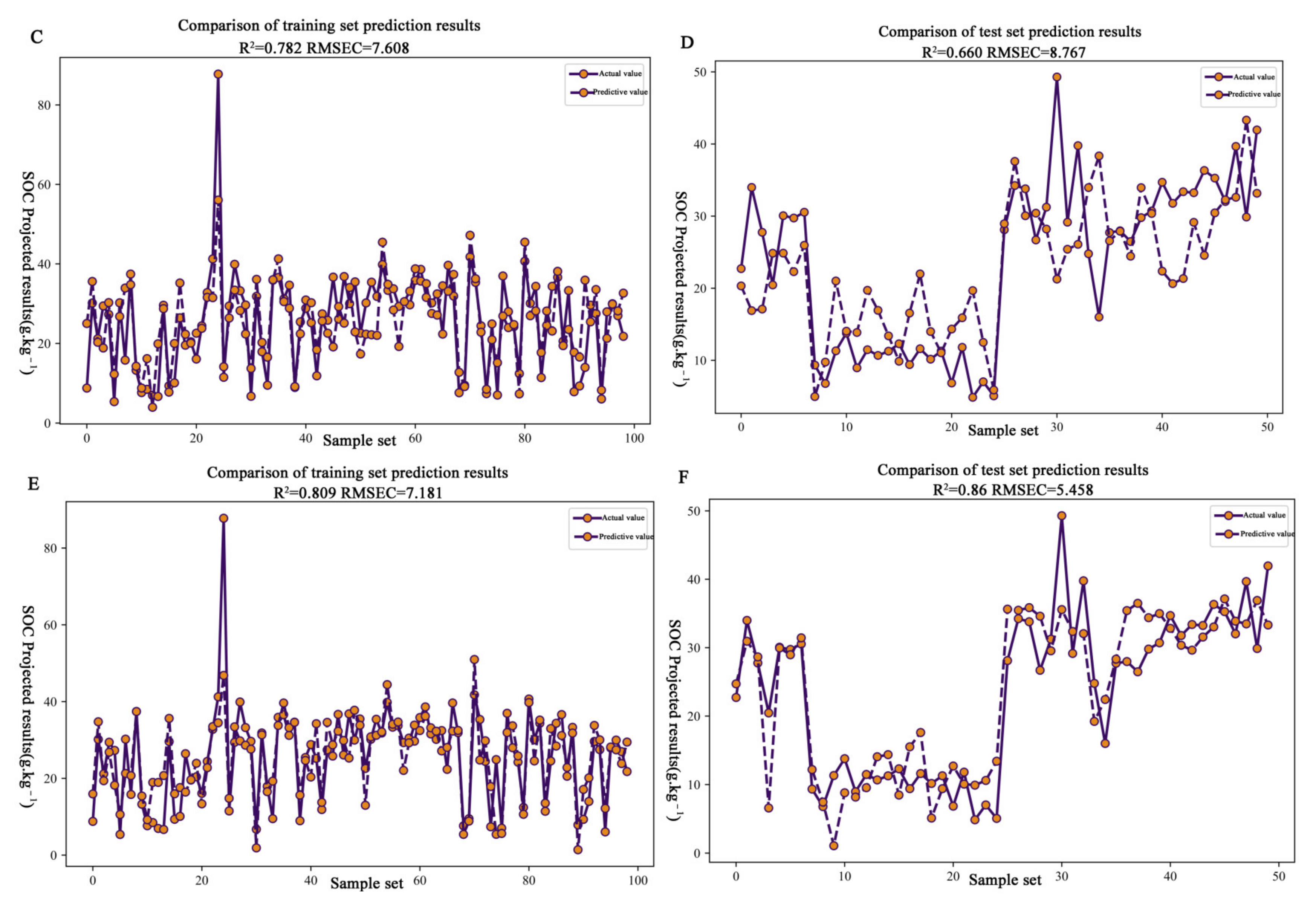
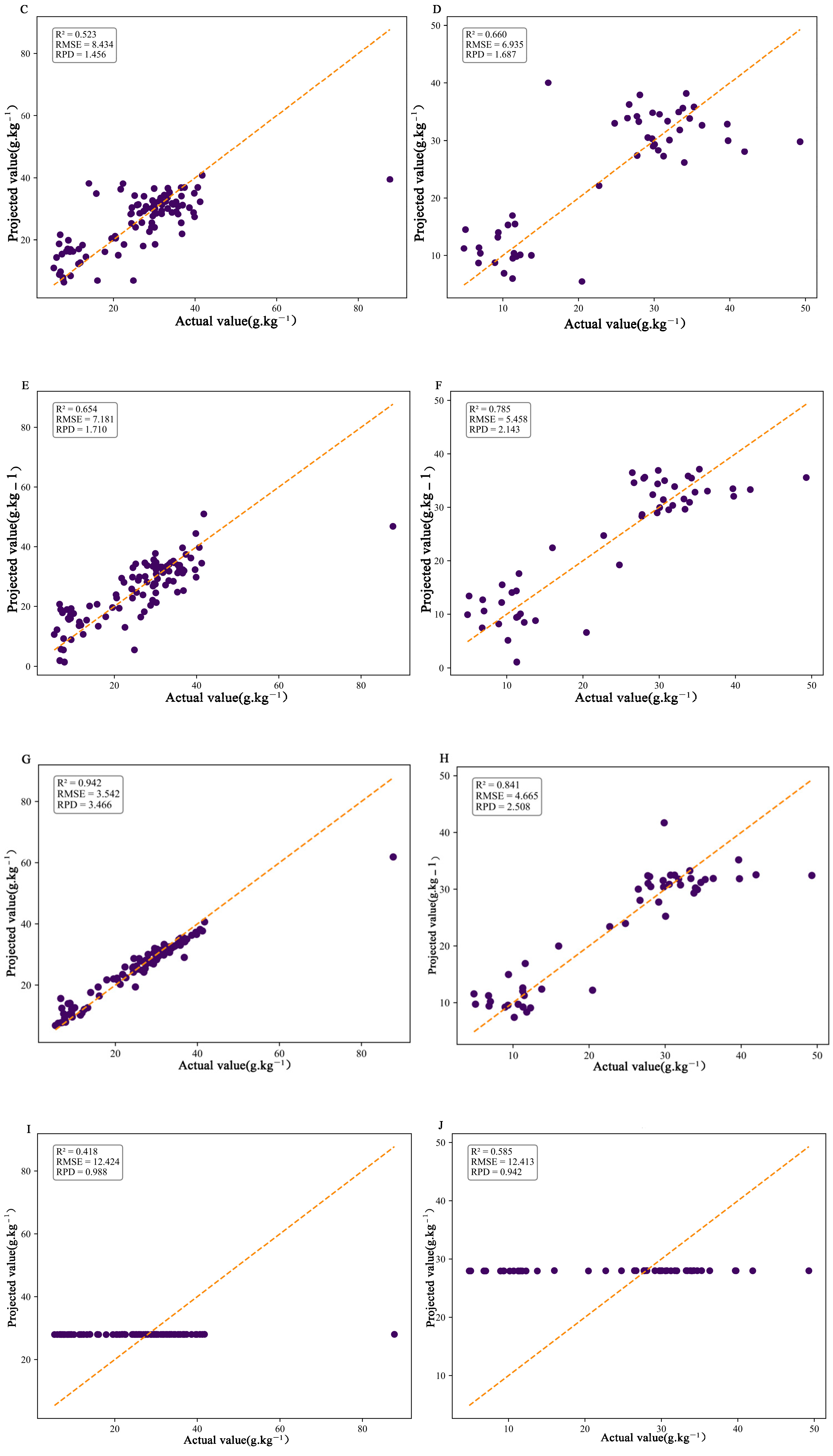
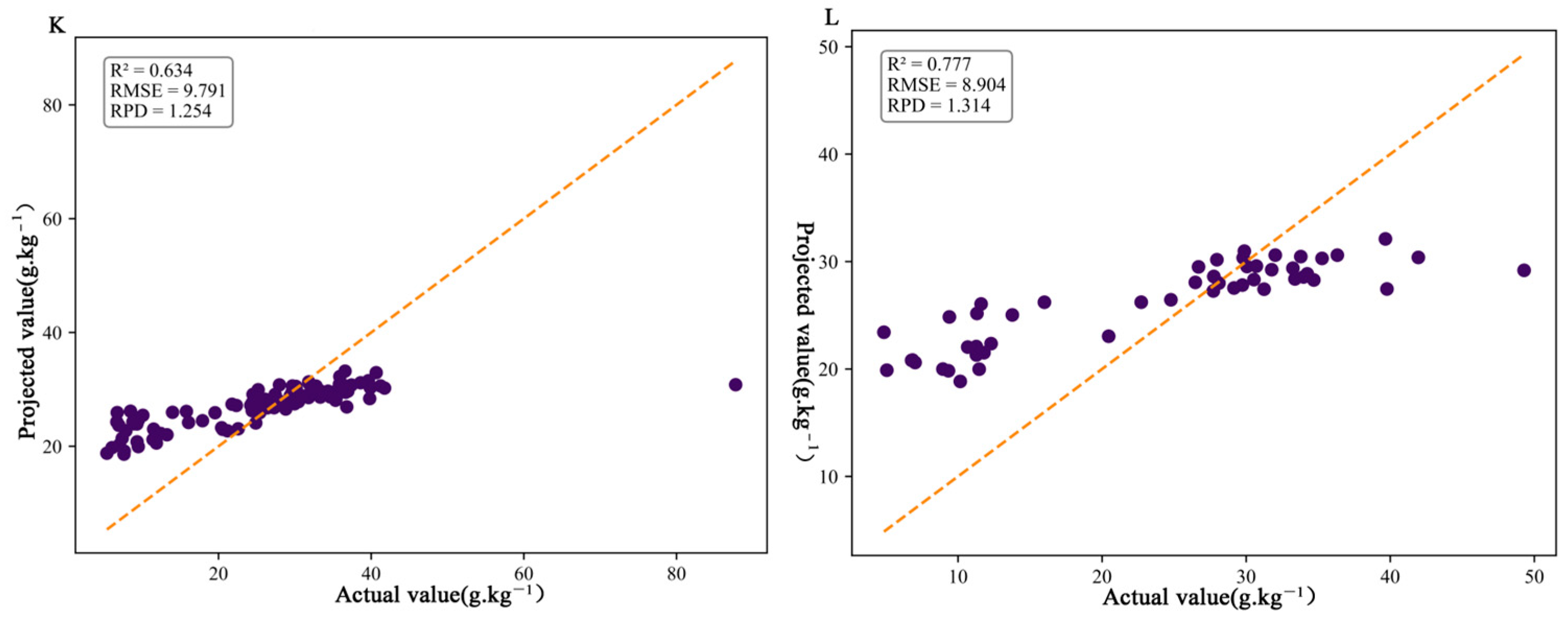
3.4. Establishment and Validation of the Estimation Model for Organic Matter Content in Citrus Soil

Based on the SPA-selected optimal feature set, six machine learning models were constructed to evaluate the predictive performance under a unified input condition. In the hyperspectral inversion of soil organic carbon (SOC) content, six different machine learning models were employed for modeling and prediction, including the Back-propagation Neural Network (BPNN), Principal Component Regression (PCR), Partial Least Squares Regression (PLSR), the Random Forest (RF), Support Vector Regression optimized by the Gray Wolf Optimizer (SVR-GWO), and Support Vector Regression (SVR). The performance of each model on the test set was evaluated using three metrics: the Coefficient of Determination (R2), Root Mean Square Error (RMSE), and Residual Prediction Deviation (RPD). The results are summarized as follows: BPNN (Figure 5A,B): R2 = 0.21, RMSE = 20.24, and RPD = 0.58; PCR (Figure 5C,D): R2 = 0.66, RMSE = 6.94, and RPD = 1.69; PLSR (Figure 5E,F): R2 = 0.79, RMSE = 5.46, and RPD = 2.14; RF (Figure 5G,H): R2 = 0.84, RMSE = 4.67, and RPD = 2.51; SVR-GWO (Figure 5I,J): R2 = 0.59, RMSE = 12.41, and RPD = 0.94; and SVR (Figure 5K,L): R2 = 0.78, RMSE = 8.90, and RPD = 1.31. The analysis results show that the RF model performed the best on the test set, with an R2 of 0.84, an RMSE of 4.67, and an RPD of 2.51, indicating high prediction accuracy and stability. According to the evaluation criteria, higher R2 and lower RMSE values indicate stronger prediction accuracy and stability; an RPD between 2.5 and 3.0 indicates good predictive capability, while an RPD below 2.0 suggests weak prediction performance [27]. Therefore, the RF model performed outstandingly on the test set and exhibited strong fitting ability on the calibration set, making it the best-performing method in SOC hyperspectral inversion. Further observation of the calibration set results shows that the RF model had an R2 of 0.94, an RMSE of 3.54, and an RPD of 3.47, indicating excellent fitting ability and stable prediction performance during the training phase. In contrast, the BPNN model performed poorly, with an R2 of only 0.20, an RMSE of 22.72, and an RPD of 0.54 on the calibration set, indicating low predictive capability in both the calibration and test sets. The PLSR model had an R2 of 0.65, an RMSE of 7.18, an RPD of 1.71 on the calibration set and an R2 of 0.79, an RMSE of 5.46, and an RPD of 2.14 on the test set. The predictive performance was moderate, consistent with research findings on PLSR application in SOC hyperspectral inversion. The PCR model had an R2 of 0.66, an RMSE of 6.94, and an RPD of 1.69 on the test set, slightly lower than PLSR. The unoptimized SVR model had an R2 of 0.63, an RMSE of 9.79, and an RPD of 1.25 on the calibration set and an R2 of 0.78, an RMSE of 8.90, and an RPD of 1.31 on the test set, showing fairly average performance. It is worth noting that although Gray Wolf Optimization (SVR-GWO) was applied to optimize the parameters of the SVR model, the calibration set’s R2 increased to 0.42. Still, the test set’s R2 was only 0.59, with a higher RMSE (12.41) and an RPD of 0.94, indicating that this optimization method did not significantly improve the prediction performance of the SVR model. Based on the modeling and prediction performance of the models, their inversion performance ranks as follows: RF > PLSR > SVR > PCR > SVR-GWO > BPNN. The results indicate that the RF model has a higher Coefficient of Determination and a lower prediction error on the test set. It demonstrates excellent fitting performance on the calibration set, making it the best and most stable method for current SOC hyperspectral inversion.

4. Discussion

4.1. Effects of Different Spectral Transformations on Modeling Accuracy

In this study, nine preprocessing methods were applied to the spectral data—including the First Derivative (FD), the Second Derivative (SD), Multiplicative Scatter Correction (MSC), Standard Normal Variate (SNV), De-trending, Normalization, Zero-centering, Savitzky–Golay smoothing (SG smoothing), and Moving Average smoothing—to construct Partial Least Squares Regression (PLSR) models. A comparative analysis of model performance under different preprocessing methods was subsequently conducted. According to the inversion results, the model constructed using the Second-Derivative (SD) method performed best on both the calibration and test sets, with an R2 of 0.886, an RMSE of 4.129, and an RPD of 2.973 on the calibration set and an R2 of 0.765, an RMSE of 5.617, and an RPD of 2.082 on the test set. Spectral preprocessing significantly improved the quality of the soil organic carbon (SOC) content prediction model. Different preprocessing methods can effectively remove noise, baseline drift, and scattering effects from the spectral data, enhancing the absorption peaks of organic carbon features, thereby improving the model’s predictive performance [28]. Commonly used preprocessing methods include the First Derivative (FD), the Second Derivative (SD), Standard Normal Variate (SNV), Multiplicative Scatter Correction (MSC), De-trending, and Normalization [29,30]. Among these, derivative transformations are particularly suitable for soil spectral analysis: The First Derivative removes baseline shifts, and the Second Derivative further eliminates linear trends while highlighting absorption peaks, generally resulting in better prediction performance [31]. Additionally, scattering correction methods (such as SNV and MSC) correct path length variations caused by particle size and moisture changes, further enhancing the correlation between spectral data and carbon content and thus improving the model’s robustness [32]. Brunet suggests that using FD for spectral transformation can effectively improve the estimation accuracy of organic carbon and nitrogen [33]. Heil et al. (2021) evaluated 55 preprocessing combinations. They found that the SOC model based on the Second Derivative combined with Savitzky–Golay smoothing achieved the highest validation accuracy (R2 = 0.94), even without additional scattering correction (such as SNV or MSC) [34], which is consistent with the results of this study. However, not all preprocessing methods improve model performance, and excessive or improper preprocessing may remove valuable information. Therefore, careful selection and optimization are necessary [35]. Overall, Second-Derivative transformations typically perform the best in SOC prediction as they effectively enhance the characteristic absorption information of organic carbon while controlling baseline interference, thereby improving modeling accuracy. Although the FD-preprocessed model showed slightly higher R2 and lower RMSE on the validation set (R2 = 0.821 and RMSE = 4.905) compared to SD (R2 = 0.765 and RMSE = 5.617), the SD model demonstrated more stable and consistent performance across both calibration and validation sets. This suggests that SD preprocessing offers better generalization capacity and reduces model overfitting, which supports its selection as the preferred method in this study.

4.2. Influence of Spectral Feature Band Selection on Modeling Accuracy

Selecting feature band extraction methods significantly affects model performance, and selecting an appropriate method can effectively enhance model accuracy. In this study, three methods—Competitive Adaptive Reweighted Sampling (CARS), Principal Component Analysis (PCA), and the Successive Projections Algorithm (SPA)—were employed to select 152, 23, and 10 feature bands, respectively, for the hyperspectral inversion of soil organic carbon (SOC) content. A comparative analysis was conducted by constructing Partial Least Squares Regression (PLSR) models, and the results indicated that the model built using the feature bands selected by the SPA method exhibited the best performance. The soil spectrum typically contains hundreds or thousands of strongly correlated wavelengths, many of which carry redundant information or noise. Therefore, reducing spectral dimensionality (whether through feature selection or transformation) is crucial for improving the performance and stability of SOC estimation models [36]. Traditional Principal Component Analysis (PCA) compresses the data into a few unrelated components (PCs), capturing most of the variability, thereby reducing multicollinearity and mitigating overfitting, typically resulting in a more streamlined model without losing excessive information [37]. For example, Jinbao Liu et al. demonstrated the feasibility of the PCR method in soil near-infrared spectroscopy and achieved good calibration accuracy for SOC by reducing the PC factor set [38]. However, the limitation of PCA is that it retains overall variability rather than targeting variables most related to SOC. As a result, some principal components extracted by PCA may be related to soil properties (such as texture, moisture, etc.) that are not directly related to organic carbon [39]. This limitation has prompted the use of supervised band selection algorithms that are specifically designed to select wavelengths most associated with SOC. Competitive Adaptive Reweighted Sampling (CARS) and the Successive Projections Algorithm (SPA) are two commonly used feature band selection methods [40]. CARS is an iterative algorithm based on the Monte Carlo method that selects wavelengths based on regression coefficients (usually in PLSR), gradually retaining or weighting those bands that contribute the most to the prediction [41]. The SPA is a forward selection method that selects wavelengths to maximize information content while minimizing multicollinearity [42]. Both methods can significantly reduce the number of input bands, removing irrelevant information and noise. Previous studies have shown that models constructed based on these selected bands usually outperform models using full-spectrum data [43,44,45]. Issam Barra compared models using the full spectrum with feature bands selected by CARS, Particle Swarm Optimization (PSO), and Ant Colony Optimization (ACO) and found that all feature band selection methods significantly reduced model complexity and improved prediction accuracy in many cases [46]. Haihui Cai’s study also showed that the three dimensionality reduction algorithms CARS, SPA, and PSO could compress spectral data to less than 10% of its original size, with selected wavelengths of 98, 156, and 102, respectively. The RPD of the validation set was greater than 1.50 for all, effectively achieving the inversion of SOC content in jujube orchards. Compared with the R combined model, the dimensionality-reduced combined model saved at least 30% in time cost [47]. These results emphasize that targeted band selection simplifies the model and filters out spectral variability unrelated to SOC, thereby improving the model’s predictive performance. In conclusion, the PCA method provides broad noise removal effects, while advanced band selection algorithms such as CARS and SPA specifically enhance information related to SOC. These two strategies have been quantitatively proven to improve the robustness and accuracy of soil carbon spectral models.

4.3. Comparison of Modeling Methods for SOC Estimation (PLSR, PCR, RF, SVR, SVR-GWO, and BPNN)

In the hyperspectral inversion of soil organic carbon (SOC) content, this study used six machine learning models for modeling and prediction, including the Back-propagation Neural Network (BPNN), Principal Component Regression (PCR), Partial Least Squares Regression (PLSR), the Random Forest (RF), Gray Wolf Optimizer–Support Vector Regression (SVR-GWO), and Support Vector Regression (SVR). A comprehensive comparison of the modeling and prediction performance of each model shows that the inversion performance ranks as follows: RF > PLSR > SVR > PCR > SVR-GWO > BPNN. The results show that the RF model not only exhibits a higher Coefficient of Determination (R2) and a lower prediction error (RMSE) on the test set but also demonstrates excellent fitting performance on the training set, making it the most effective and stable method for the hyperspectral inversion of SOC content in citrus soils. Numerous regression and machine learning methods have been applied in SOC prediction, with Partial Least Squares Regression (PLSR) being the most widely used method in soil spectroscopy [14]. Previous studies have shown that PLSR achieves good accuracy in SOC prediction. For example, Nuwan K modeled predicted organic and total carbon (TC) in the continental United States using VisNIR spectroscopy, with local PLSR models performing best in horizon and texture aspects [48]. Typically, PLSR outperforms PCR because PLSR maximizes the covariance with the target variable, rather than just the spectral variance. However, both PLSR and PCR are linear methods and may face challenges when complex nonlinear relationships exist between the data [49]. To capture the more complicated relationships between spectra and SOC, nonlinear machine learning models such as Support Vector Regression (SVR), the Random Forest (RF), and Artificial Neural Networks (ANNs) have been widely explored. Studies show that SVR with the Radial Basis Function (RBF) kernel often performs better or even more accurately than PLSR models in soil studies. For example, Kennedy and Were found that the Support Vector Regression model performed best in the spatial prediction of SOC stocks, with the Artificial Neural Network model following closely behind [50]. Emna Karray found that SVR outperformed PLSR in both C1 (0% IS, 100% LS) and C5 (100% IS, 0% LS) cases, with R2 values of 0.79 and 0.76 and RMSE values of 1.42 and 1.3, respectively [51]. Furthermore, the model combining Gray Wolf Optimization (GWO) with SVR (SVR-GWO) further improves model performance by optimizing the hyperparameters of SVR or selecting features. For example, in some applications, the SVR-GWO-optimized model achieved a higher Coefficient of Determination and a smaller prediction error than the baseline SVR, RF, or PLSR models when predicting soil heavy metal content [52]. The Random Forest (RF) has shown superior performance as an ensemble tree method because it can model interactions and nonlinear effects between variables and is less sensitive to high-dimensional data [53]. Said Nawar compared the RF, ANN, and Gradient Boosting Machine (GBM) in the online prediction of total nitrogen (TN) and total carbon (TC) in soil, showing that the RF model generally outperforms the GBM and ANN in cross-validation, laboratory, and online predictions, particularly when using a broader European dataset [54]. Luthfan Nur Habibi’s research also shows that RF regression outperforms PLS regression in all predictor variable combinations, especially in training and testing datasets. Artificial neural networks, such as Back-Propagation Neural Networks (BPNNs), add another powerful option, as they are capable of approximating complex functional relationships given sufficient data [55]. A study published in Scientific Reports showcased that ANNs trained on extensive and varied datasets achieved a 98.9% accuracy rate in spectroscopic classification tasks, correctly predicting at least 4450 out of 4500 samples in the test set [56]. In summary, various machine learning models show different advantages in SOC content prediction. The RF and SVR excel at capturing nonlinear relationships, and SVR-GWO further improves SVR’s performance through optimization. At the same time, PLSR and PCR are suitable for scenarios with more linear data relationships and higher interpretability requirements. Although the BPNN has powerful nonlinear modeling capabilities, it performed relatively weakly in this study. Therefore, the RF is the most effective and stable citrus SOC hyperspectral inversion model.

5. Conclusions

This study proposes a scientifically rigorous and practically applicable multi-stage framework for soil organic carbon (SOC) estimation based on Fourier Transform Infrared (FTIR) spectroscopy. By integrating spectral preprocessing, variable selection, and machine learning modeling into a unified pipeline, the framework addresses both the complexity of spectral data and the demand for predictive robustness in heterogeneous soil environments. Among the nine preprocessing techniques evaluated, the second-derivative (SD) transformation consistently delivered superior performance by significantly enhancing the signal-to-noise ratio and amplifying diagnostic absorption features, laying a solid foundation for subsequent modeling. When combined with the Successive Projections Algorithm (SPA) for feature selection, the framework achieved over 98% dimensionality reduction—retaining only 10 key wavenumbers—while effectively preserving the core spectral information. The resulting SD–SPA–Random Forest (RF) model demonstrated outstanding predictive capacity, achieving an R2 of 0.84 and an RPD of 2.51 on the independent test set, clearly outperforming conventional full-spectrum Partial Least Squares Regression (PLSR) and neural network models. Compared to traditional visible–near-infrared (Vis–NIR) methods, FTIR exhibited distinct advantages in chemical specificity. By directly capturing the vibrational signals of SOC-characteristic functional groups such as C=O, O–H, and C–O, FTIR provided higher spectral resolution and stability under complex field conditions. To ensure model robustness, 149 soil samples encompassing a wide SOC concentration range (4.86–87.75 g/kg) and pronounced spatial heterogeneity were stratified using the Kennard–Stone algorithm, maintaining consistent statistical distributions between the calibration and validation sets. The proposed framework adopts a modular architecture with strong scalability, enabling full-process implementation from field sampling to spectral analysis and model inference. It is well suited for real-world applications such as high-resolution SOC mapping, precision fertilization, and data-driven orchard nutrient management. Future research should prioritize enhancing cross-regional generalizability by incorporating key environmental covariates (e.g., soil texture, moisture, and topographic gradients) and applying transfer learning strategies. Overall, this interpretable and generalizable modeling paradigm provides a robust scientific basis and technical support for digital soil assessments and sustainable orchard management.
In conclusion, this research demonstrates the value of a systemically integrated and intelligent modeling framework for SOC estimation in orchard soils. The proposed approach provides a scalable and adaptive tool for precision carbon monitoring and management, contributing to advancing digital soil science and remote sensing–based agricultural modeling.

Author Contributions

Methodology, Y.W. and X.M.; formal analysis, Y.W.; investigation, Y.W., X.M., S.Y., S.W., H.C., Y.Q. and Z.Z.; data curation, Y.W., S.Y. and X.M.; writing—review and editing, Y.W., X.M. and S.Y.; supervision, Y.W. All authors have read and agreed to the published version of the manuscript.

Funding

This research was funded by the Guangxi Smart Citrus Industry Key Technology Research, Development, and Integrated Demonstration Project (Grant No. Guike AA20108003), the Guangxi Academy of Agricultural Sciences Basic Research Fund (Grant No. 2025YP061), the Guangxi Major Science and Technology Project (Grant No. AA22036002), and the Guangxi Academy of Agricultural Sciences Basic Research Fund (Grant No. 2021YT084).

Institutional Review Board Statement

Not applicable.

Data Availability Statement

Data are contained within the article.

Acknowledgments

The author acknowledges the use of Grammarly (Grammarly Inc., www.grammarly.com) for minor grammatical corrections. All AI-assisted suggestions were manually reviewed to ensure accuracy. No content was generated by AI tools. The author confirms that all individuals included in this section have consented to the acknowledgment.

Conflicts of Interest

The authors declare no conflicts of interest.

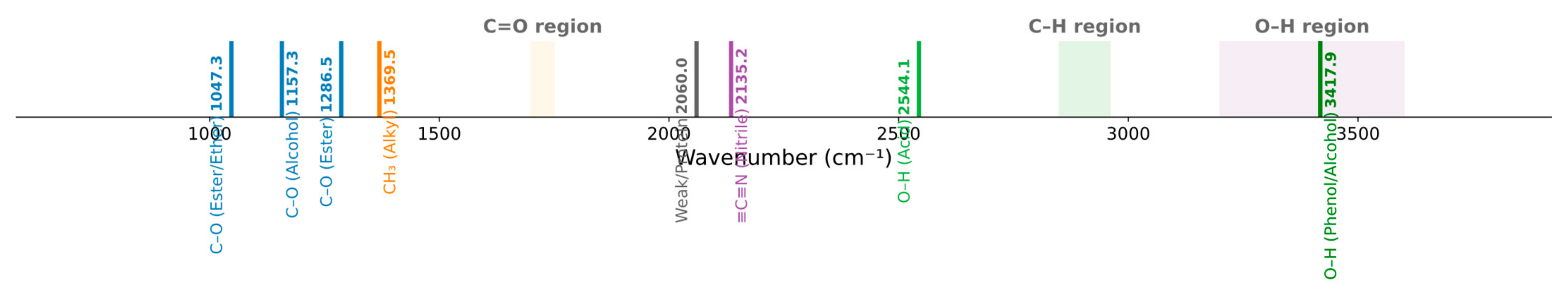
Appendix A. Interpretation of SPA-Selected Features

Figure A1. SPA-selected bands overlaid on FTIR functional group regions. Key alignments were observed in the C–O and O–H regions.
Agriculture 15 01417 g0a1
Figure A2. PLSR loadings of PC1 and PC2 with SPA-selected features highlighted, showing correspondence with major loading peaks.
Agriculture 15 01417 g0a2
Table A1. SPA-selected wavenumbers and assigned functional groups.
SPA Wavenumber (cm−1)Assigned Functional GroupIR Region (cm−1)Chemical Relevance
1047.35C–O stretch (ester/ether)1000–1300Relevant (SOM signature)
538.14Possible halide (C–Br)500–600Low relevance
3417.86O–H stretch (phenol/alcohol)3200–3600Relevant (hydroxyl)
1286.52C–O stretch (ester)1200–1300Relevant (ester components)
1157.29C–O stretch (alcohol)1100–1200Relevant (alcohol indicators)
1369.46CH3 bend (alkyl)1350–1400Relevant (alkyl side chains)
3996.51Instrument edge/noise>3800Ignore (out of range)
2135.2C≡C or C≡N stretch (alkyne/nitrile)2100–2260Possible trace group
2544.11O–H broad tail (carboxylic acid)2500–3300Relevant (acidic region)
2059.98Weak signal/uncertain2000–2100Uncertain

References

  1. Gao, G.; Li, G.; Liu, M.; Liu, J.; Ma, S.; Li, D.; Liang, X.; Wu, M.; Li, Z. Microbial Carbon Metabolic Activity and Bacterial Cross-Profile Network in Paddy Soils of Different Fertility. Appl. Soil Ecol. 2024, 195, 105233. [Google Scholar] [CrossRef]
  2. Trivedi, P.; Singh, B.P.; Singh, B.K. Soil Carbon. In Soil Carbon Storage; Elsevier: Amsterdam, The Netherlands, 2018; pp. 1–28. ISBN 978-0-12-812766-7. [Google Scholar]
  3. Dusenge, M.E.; Duarte, A.G.; Way, D.A. Plant Carbon Metabolism and Climate Change: Elevated CO2 and Temperature Impacts on Photosynthesis, Photorespiration and Respiration. New Phytol. 2019, 221, 32–49. [Google Scholar] [CrossRef] [PubMed]
  4. Wang, B.; An, S.; Liang, C.; Liu, Y.; Kuzyakov, Y. Microbial Necromass as the Source of Soil Organic Carbon in Global Ecosystems. Soil Biol. Biochem. 2021, 162, 108422. [Google Scholar] [CrossRef]
  5. Zhao, H.; Dong, Z.; Liu, B.; Xiong, H.; Guo, C.; Lakshmanan, P.; Wang, X.; Chen, X.; Shi, X.; Zhang, F.; et al. Can Citrus Production in China Become Carbon-Neutral? A Historical Retrospect and Prospect. Agric. Ecosyst. Environ. 2023, 348, 108412. [Google Scholar] [CrossRef]
  6. Yun, S.-M.; Kim, C.-S.; Lee, J.-J.; Chung, J.-S. Application of ATR-FTIR Spectroscopy for Analysis of Salt Stress in Brussels Sprouts. Metabolites 2024, 14, 470. [Google Scholar] [CrossRef]
  7. Gong, Y.; Chen, X.; Wu, W. Application of Fourier Transform Infrared (FTIR) Spectroscopy in Sample Preparation: Material Characterization and Mechanism Investigation. Adv. Sample Prep. 2024, 11, 100122. [Google Scholar] [CrossRef]
  8. Buja, I.; Sabella, E.; Monteduro, A.G.; Chiriacò, M.S.; De Bellis, L.; Luvisi, A.; Maruccio, G. Advances in Plant Disease Detection and Monitoring: From Traditional Assays to In-Field Diagnostics. Sensors 2021, 21, 2129. [Google Scholar] [CrossRef]
  9. Zhang, J.; Huang, Y.; Pu, R.; Gonzalez-Moreno, P.; Yuan, L.; Wu, K.; Huang, W. Monitoring Plant Diseases and Pests through Remote Sensing Technology: A Review. Comput. Electron. Agric. 2019, 165, 104943. [Google Scholar] [CrossRef]
  10. Muneer, M.A.; Afridi, M.S.; Saddique, M.A.B.; Chen, X.; Nisa, Z.U.; Yan, X.; Farooq, I.; Munir, M.Z.; Yang, W.; Ji, B.; et al. Nutrient Stress Signals: Elucidating the Morphological, Physiological, and Molecular Responses of Fruit Trees to Macronutrient Deficiency and Their Management Strategies. Sci. Hortic. 2024, 329, 112985. [Google Scholar] [CrossRef]
  11. Margenot, A.J.; Parikh, S.J.; Calderón, F.J. Fourier-transform Infrared Spectroscopy for Soil Organic Matter Analysis. Soil Sci. Soc. Amer. J. 2023, 87, 1503–1528. [Google Scholar] [CrossRef]
  12. Li, X.; McCarty, G.W. Use of Principal Components for Scaling Up Topographic Models to Map Soil Redistribution and Organic Carbon. JoVE 2018, 140, 58189. [Google Scholar] [CrossRef]
  13. Bian, Z.; Guo, X.; Wang, S.; Zhuang, Q.; Jin, X.; Wang, Q.; Jia, S. Applying Statistical Methods to Map Soil Organic Carbon of Agricultural Lands in Northeastern Coastal Areas of China. Arch. Agron. Soil Sci. 2020, 66, 532–544. [Google Scholar] [CrossRef]
  14. Das, B.; Chakraborty, D.; Singh, V.K.; Das, D.; Sahoo, R.N.; Aggarwal, P.; Murgaokar, D.; Mondal, B.P. Partial Least Squares Regression-Based Machine Learning Models for Soil Organic Carbon Prediction Using Visible–Near Infrared Spectroscopy. Geoderma Reg. 2023, 33, e00628. [Google Scholar] [CrossRef]
  15. Emadi, M.; Taghizadeh-Mehrjardi, R.; Cherati, A.; Danesh, M.; Mosavi, A.; Scholten, T. Predicting and Mapping of Soil Organic Carbon Using Machine Learning Algorithms in Northern Iran. Remote. Sens. 2020, 12, 2234. [Google Scholar] [CrossRef]
  16. Li, Y.; Yao, G.; Li, S.; Dong, X. Predicting and Mapping of Soil Organic Matter with Machine Learning in the Black Soil Region of the Southern Northeast Plain of China. Agronomy 2025, 15, 533. [Google Scholar] [CrossRef]
  17. Chen, Q.; Wang, Y.; Zhu, X. Soil Organic Carbon Estimation Using Remote Sensing Data-Driven Machine Learning. PeerJ 2024, 12, e17836. [Google Scholar] [CrossRef]
  18. Meng, W. Risk Perception and Influencing Factors of Citrus Growers. Master’s Thesis, Guangxi University, Nanning, China, 2023. (In Chinese) [Google Scholar] [CrossRef]
  19. Qi, Z. Hyperspectral Inversion Method for Estimating Orchard Soil Organic Carbon Content. Master’s Thesis, Shandong Agricultural University, Taian, China, 2023. (In Chinese). [Google Scholar]
  20. Yang, D.; Hu, J. A Detection Method of Oil Content for Maize Kernels Based on CARS Feature Selection and Deep Sparse Autoencoder Feature Extraction. Ind. Crops Prod. 2024, 222, 119464. [Google Scholar] [CrossRef]
  21. Liu, K.; Chen, X.; Li, L.; Chen, H.; Ruan, X.; Liu, W. A Consensus Successive Projections Algorithm—Multiple Linear Regression Method for Analyzing near Infrared Spectra. Anal. Chim. Acta 2015, 858, 16–23. [Google Scholar] [CrossRef]
  22. Ma, J.; Yuan, Y. Dimension Reduction of Image Deep Feature Using PCA. J. Vis. Commun. Image Represent. 2019, 63, 102578. [Google Scholar] [CrossRef]
  23. Malgady, R.G.; Krebs, D.E. Understanding Correlation Coefficients and Regression. Phys. Ther. 1986, 66, 110–120. [Google Scholar] [CrossRef]
  24. Williams, P.C.; Sobering, D.C. Comparison of Commercial near Infrared Transmittance and Reflectance Instruments for Analysis of Whole Grains and Seeds. J. Near Infrared Spectrosc. 1993, 1, 25–32. [Google Scholar] [CrossRef]
  25. Zheng, J.Y.; Zhao, J.S.; Shi, Z.H.; Wang, L. Soil aggregates are key factors that regulate erosion-related carbon loss in citrus orchards of southern China: Bare land vs. grass-covered land. Agric. Ecosyst. Environ. 2021, 309, 107254. [Google Scholar] [CrossRef]
  26. Yao, X.; Yu, K.; Deng, Y.; Liu, J.; Lai, Z. Spatial variability of soil organic carbon and total nitrogen in the hilly red soil region of Southern China. J. For. Res. 2020, 31, 2385–2394. [Google Scholar] [CrossRef]
  27. Saeys, Y.; Inza, I.; Larrañaga, P. A Review of Feature Selection Techniques in Bioinformatics. Bioinformatics 2007, 23, 2507–2517. [Google Scholar] [CrossRef]
  28. Zhang, Z.; Ding, J.; Wang, J.; Ge, X. Prediction of Soil Organic Matter in Northwestern China Using Fractional-Order Derivative Spectroscopy and Modified Normalized Difference Indices. CATENA 2020, 185, 104257. [Google Scholar] [CrossRef]
  29. Lee, L.C.; Liong, C.-Y.; Jemain, A.A. A Contemporary Review on Data Preprocessing (DP) Practice Strategy in ATR-FTIR Spectrum. Chemom. Intell. Lab. Syst. 2017, 163, 64–75. [Google Scholar] [CrossRef]
  30. Jiao, Y.; Li, Z.; Chen, X.; Fei, S. Preprocessing Methods for Near-infrared Spectrum Calibration. J. Chemom. 2020, 34, e3306. [Google Scholar] [CrossRef]
  31. Gholizadeh, A.; Borůvka, L.; Saberioon, M.M.; Kozák, J.; Vašát, R.; Němeček, K. Comparing Different Data Preprocessing Methods for Monitoring Soil Heavy Metals Based on Soil Spectral Features. Soil Water Res. 2015, 10, 218–227. [Google Scholar] [CrossRef]
  32. Zhang, Z.; Chang, Z.; Huang, J.; Leng, G.; Xu, W.; Wang, Y.; Xie, Z.; Yang, J. Enhancing Soil Texture Classification with Multivariate Scattering Correction and Residual Neural Networks Using Visible Near-Infrared Spectra. J. Environ. Manag. 2024, 352, 120094. [Google Scholar] [CrossRef]
  33. Brunet, D.; Barthès, B.G.; Chotte, J.-L.; Feller, C. Determination of Carbon and Nitrogen Contents in Alfisols, Oxisols and Ultisols from Africa and Brazil Using NIRS Analysis: Effects of Sample Grinding and Set Heterogeneity. Geoderma 2007, 139, 106–117. [Google Scholar] [CrossRef]
  34. Heil, K.; Schmidhalter, U. An Evaluation of Different NIR-Spectral Pre-Treatments to Derive the Soil Parameters C and N of a Humus-Clay-Rich Soil. Sensors 2021, 21, 1423. [Google Scholar] [CrossRef] [PubMed]
  35. Rosin, N.A.; Dalmolin, R.S.D.; Horst-Heinen, T.Z.; Moura-Bueno, J.M.; Silva-Sangoi, D.V.D.; Silva, L.S.D. Diffuse Reflectance Spectroscopy for Estimating Soil Organic Carbon and Making Nitrogen Recommendations. Sci. Agric. 2021, 78, e20190246. [Google Scholar] [CrossRef]
  36. Yang, S.; Wang, Z.; Ji, C.; Hao, Y.; Liang, Z.; Yan, X.; Qiao, X.; Feng, M.; Xiao, L.; Song, X.; et al. Efficient Prediction of SOC and Aggregate OC Components by Continuous Wavelet Transform Spectra under Different Feature Selection Methods. Comput. Electron. Agric. 2024, 217, 108550. [Google Scholar] [CrossRef]
  37. Salem, N.; Hussein, S. Data Dimensional Reduction and Principal Components Analysis. Procedia Comput. Sci. 2019, 163, 292–299. [Google Scholar] [CrossRef]
  38. Liu, J.; Han, J.; Zhang, Y.; Wang, H.; Kong, H.; Shi, L. Prediction of Soil Organic Carbon with Different Parent Materials Development Using Visible-near Infrared Spectroscopy. Spectrochim. Acta Part A Mol. Biomol. Spectrosc. 2018, 204, 33–39. [Google Scholar] [CrossRef]
  39. Jolliffe, I.T.; Cadima, J. Principal Component Analysis: A Review and Recent Developments. Phil. Trans. R. Soc. A. 2016, 374, 20150202. [Google Scholar] [CrossRef]
  40. Tang, G.; Huang, Y.; Tian, K.; Song, X.; Yan, H.; Hu, J.; Xiong, Y.; Min, S. A New Spectral Variable Selection Pattern Using Competitive Adaptive Reweighted Sampling Combined with Successive Projections Algorithm. Analyst 2014, 139, 4894. [Google Scholar] [CrossRef]
  41. Li, H.; Liang, Y.; Xu, Q.; Cao, D. Key Wavelengths Screening Using Competitive Adaptive Reweighted Sampling Method for Multivariate Calibration. Anal. Chim. Acta 2009, 648, 77–84. [Google Scholar] [CrossRef]
  42. Galvão, R.K.H.; Araújo, M.C.U.; Fragoso, W.D.; Silva, E.C.; José, G.E.; Soares, S.F.C.; Paiva, H.M. A Variable Elimination Method to Improve the Parsimony of MLR Models Using the Successive Projections Algorithm. Chemom. Intell. Lab. Syst. 2008, 92, 83–91. [Google Scholar] [CrossRef]
  43. Ayna, C.O.; Mdrafi, R.; Du, Q.; Gurbuz, A.C. Learning-Based Optimization of Hyperspectral Band Selection for Classification. Remote Sens. 2023, 15, 4460. [Google Scholar] [CrossRef]
  44. Zheng, Z.; Liu, Y.; He, M.; Chen, D.; Sun, L.; Zhu, F. Effective Band Selection of Hyperspectral Image by an Attention Mechanism-Based Convolutional Network. RSC Adv. 2022, 12, 8750–8759. [Google Scholar] [CrossRef] [PubMed]
  45. Mukherjee, R.; Liu, D. Downscaling MODIS Spectral Bands Using Deep Learning. GIScience Remote Sens. 2021, 58, 1300–1315. [Google Scholar] [CrossRef]
  46. Barra, I.; Haefele, S.M.; Sakrabani, R.; Kebede, F. Soil Spectroscopy with the Use of Chemometrics, Machine Learning and Pre-Processing Techniques in Soil Diagnosis: Recent Advances–A Review. TrAC Trends Anal. Chem. 2021, 135, 116166. [Google Scholar] [CrossRef]
  47. Cai, H.; Zhou, L.; Shi, Z.; Ji, W.; Luo, D.; Peng, J.; Feng, C. Hyperspectral Inversion of Soil Organic Matter in Southern Xinjiang Jujube Orchards Using the CARS-BPNN Model. Spectrosc. Spectr. Anal. 2023, 43, 2568–2573. [Google Scholar]
  48. Wijewardane, N.K.; Ge, Y.; Wills, S.; Loecke, T. Prediction of Soil Carbon in the Conterminous United States: Visible and Near Infrared Reflectance Spectroscopy Analysis of the Rapid Carbon Assessment Project. Soil Sci. Soc. Amer. J. 2016, 80, 973–982. [Google Scholar] [CrossRef]
  49. Engelen, S.; Hubert, M.; Vanden Branden, K.; Verboven, S. Robust PCR and Robust PLSR: A Comparative Study. In Theory and Applications of Recent Robust Methods; Hubert, M., Pison, G., Struyf, A., Van Aelst, S., Eds.; Birkhäuser Basel: Basel, Switzerland, 2004; pp. 105–117. ISBN 978-3-0348-9636-8. [Google Scholar]
  50. Were, K.; Bui, D.T.; Dick, Ø.B.; Singh, B.R. A Comparative Assessment of Support Vector Regression, Artificial Neural Networks, and Random Forests for Predicting and Mapping Soil Organic Carbon Stocks across an Afromontane Landscape. Ecol. Indic. 2015, 52, 394–403. [Google Scholar] [CrossRef]
  51. Karray, E.; Elmannai, H.; Toumi, E.; Hedi Gharbia, M.; Meshoul, S.; Aichi, H.; Ben Rabah, Z. Evaluating the Potentials of PLSR and SVR Models for Soil Properties Prediction Using Field Imaging, Laboratory VNIR Spectroscopy and Their Combination. Comput. Model. Eng. Sci. 2023, 136, 1399–1425. [Google Scholar] [CrossRef]
  52. Chen, Y.; Zhang, C.; Xiao, C.; Zhao, X.; Shi, Y.; Yang, H.; Liu, Z.; Li, S. Study on Prediction Model of Soil Cadmium Content, Moisture Content Correction Based on GWO-SVR. Acta Opt. Sin. 2020, 40, 1030002. (In Chinese) [Google Scholar] [CrossRef]
  53. Chan, J.C.-W.; Paelinckx, D. Evaluation of Random Forest and Adaboost Tree-Based Ensemble Classification and Spectral Band Selection for Ecotope Mapping Using Airborne Hyperspectral Imagery. Remote Sens. Environ. 2008, 112, 2999–3011. (In Chinese) [Google Scholar] [CrossRef]
  54. Nawar, S.; Mouazen, A. Comparison between Random Forests, Artificial Neural Networks and Gradient Boosted Machines Methods of On-Line Vis-NIR Spectroscopy Measurements of Soil Total Nitrogen and Total Carbon. Sensors 2017, 17, 2428. [Google Scholar] [CrossRef]
  55. Goh, A.T.C. Back-Propagation Neural Networks for Modeling Complex Systems. Artif. Intell. Eng. 1995, 9, 143–151. [Google Scholar] [CrossRef]
  56. Schuetzke, J.; Szymanski, N.J.; Reischl, M. Validating Neural Networks for Spectroscopic Classification on a Universal Synthetic Dataset. NPJ Comput. Mater. 2023, 9, 100. [Google Scholar] [CrossRef]
Figure 1. Location of the research area.
Agriculture 15 01417 g001
Figure 2. SOC spectral curve after treatment of FD (A), SD (B), MSC (C), SNV (D), De-trending (E), Zero-centered (F), Normalization (G), SG smoothing (H), and Moving Average (I).
Agriculture 15 01417 g002
Figure 3. Spectral feature selection processes and CARS, PCA, and SPA outcomes. (A) The RMSECV trend across 100 iterations in the CARS algorithm. (B) Selected variables (n = 152) at the optimal iteration in CARS. (C) Variance is explained by the first three principal components of the PCA. (D) Selected variables (n = 23) based on the top three PCs in PCA. (E) The SPA model’s RMSEP curve versus the number of selected variables. (F) Final selected variables (n = 10) by SPA.
Agriculture 15 01417 g003
Figure 4. PLSR modeling results based on CARS (A,B), PCA (C,D), and SPA (E,F).
Agriculture 15 01417 g004aAgriculture 15 01417 g004b
Figure 5. Scatter plots comparing predicted versus actual SOC content (g/kg) using six modeling algorithms on the calibration and test sets. The models include: (A,B) BPNN; (C,D) PCR; (E,F) PLSR; (G,H) RF; (I,J) SVR-GWO; and (K,L) SVR. Dashed lines represent the 1:1 line. Each subfigure reports the R2, RMSE, and RPD values.
Agriculture 15 01417 g005aAgriculture 15 01417 g005bAgriculture 15 01417 g005c
Table 1. Statistical characteristics of soil organic carbon content in citrus soils from different datasets.
DatasetNumber of SamplesMinimum (g/kg)Maximum (g/kg)Mean (g/kg)Standard DeviationCoefficient of Variation
Total Samples1494.8687.7524.9112.090.49
Calibration Set995.3887.7525.6312.280.48
Validation Set504.8649.2923.4611.700.50
Table 2. Accuracy metrics of PLSR models under different preprocessing methods.
MethodR2cRMSECRPDCR2pRMSEPRPDP
FD0.775.8522.0980.8214.9052.385
SD0.8864.1292.9730.7655.6172.082
MSC0.667.1271.7230.7345.9711.959
SNV0.6956.7411.8210.7745.512.123
De-trending0.6237.5031.6360.6676.6811.751
Normalization0.597.8191.570.6746.6111.769
Zero-centered0.5887.8391.5660.6896.4551.812
SG smoothing0.5348.3341.4730.6247.1041.646
Moving average0.5348.3341.4730.6247.1011.647
RMSEC: Root Mean Square Error of the Calibration Set; RMSEP: Root Mean Square Error of the Prediction Set; R2c: Coefficient of Determination of the Calibration Set; R2p: Coefficient of Determination of the Prediction Set. RPDC: Ratio of Performance to Deviation (Calibration Set); RPDP: Ratio of Performance to Deviation (Validation Set).
Table 3. PLSR modeling results of different variable screening methods.
Filtering MethodThe Number of VariablesCalibration SetTest Set
R2RMSERPDR2RMSERPD
CARS1520.963.364.080.866.121.89
PCA230.787.611.610.668.771.32
SPA100.817.181.70.895.462.12
Disclaimer/Publisher’s Note: The statements, opinions and data contained in all publications are solely those of the individual author(s) and contributor(s) and not of MDPI and/or the editor(s). MDPI and/or the editor(s) disclaim responsibility for any injury to people or property resulting from any ideas, methods, instructions or products referred to in the content.

