
Prediction of Soybean Yield at the County Scale Based on Multi-Source Remote-Sensing Data and Deep Learning Models

 and
and
Abstract
1. Introduction
2. Materials and Methods
2.1. Study Area
2.2. Dataset and Preprocessing
2.2.1. Vegetation Indices
2.2.2. Environmental Data
2.2.3. Photosynthetic Parameters
2.3. Yield Prediction Model
2.3.1. RFR
2.3.2. SVR
2.3.3. XGBoost
2.3.4. CNN
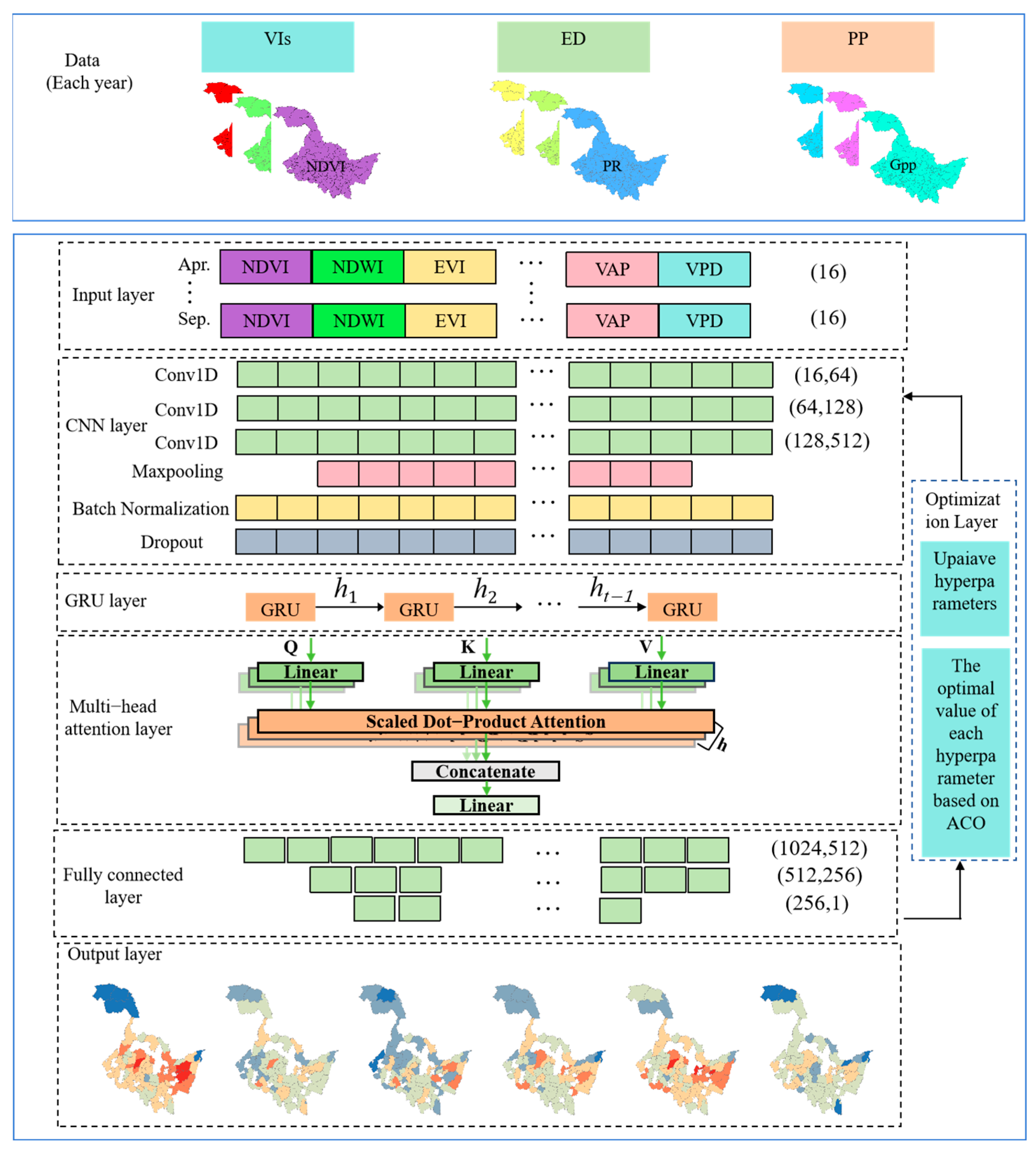
2.3.5. ACGM
2.4. Model Evaluation Indicators
3. Results
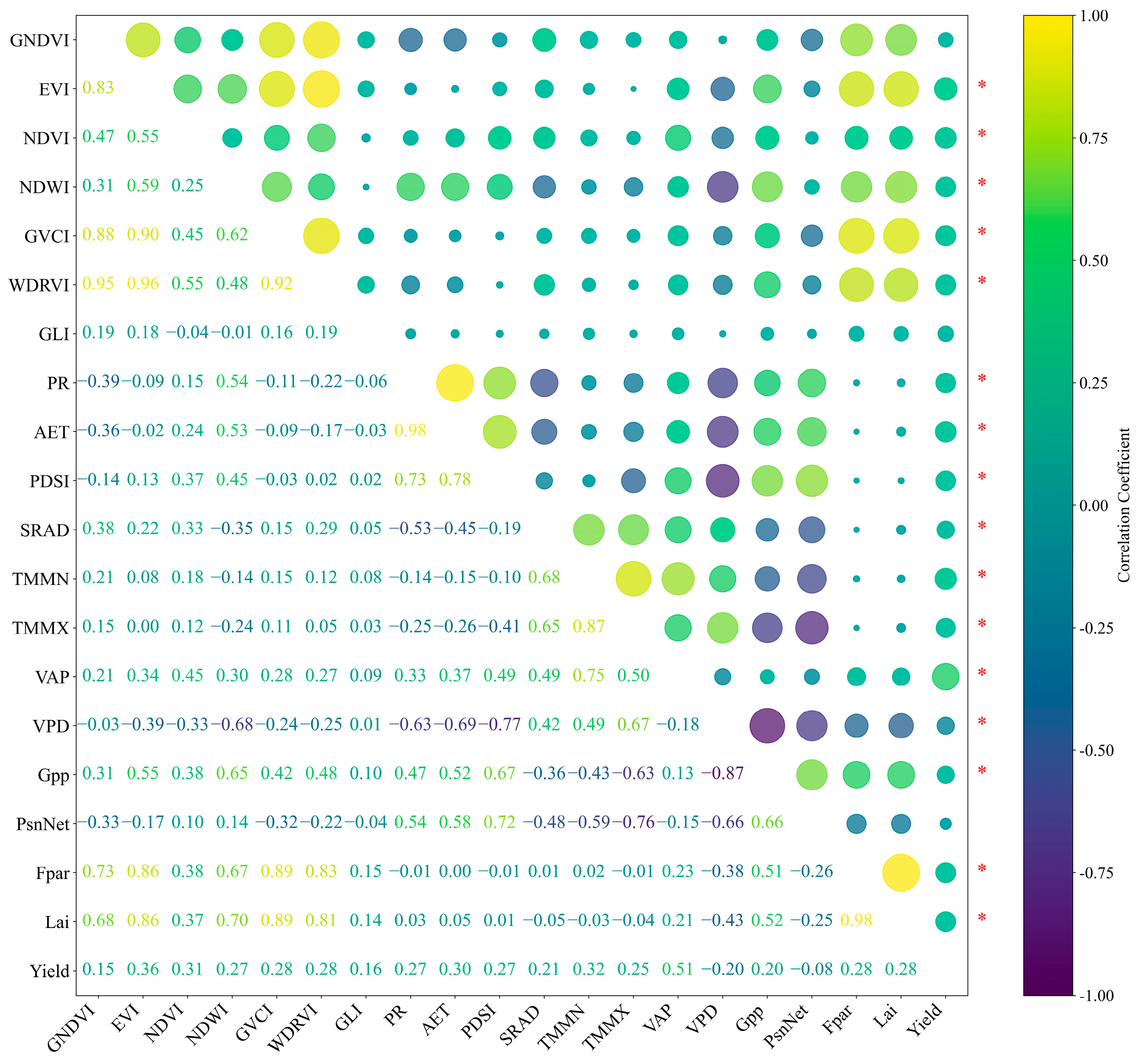
3.1. Correlation Analysis Between Variables and Yield
3.2. Comparison of Soybean Yield Prediction Models
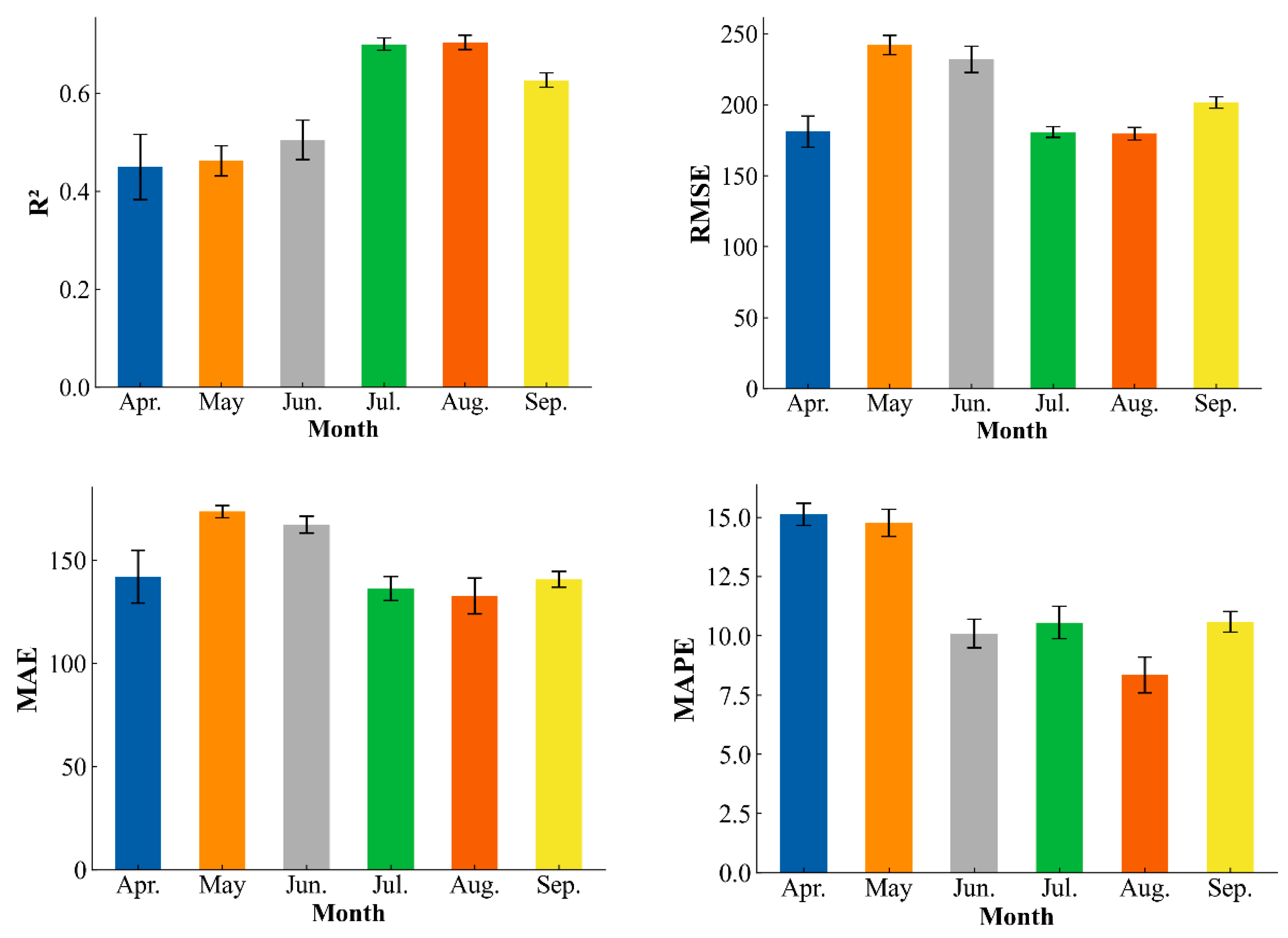
3.3. Optimal Month for Soybean Yield Prediction
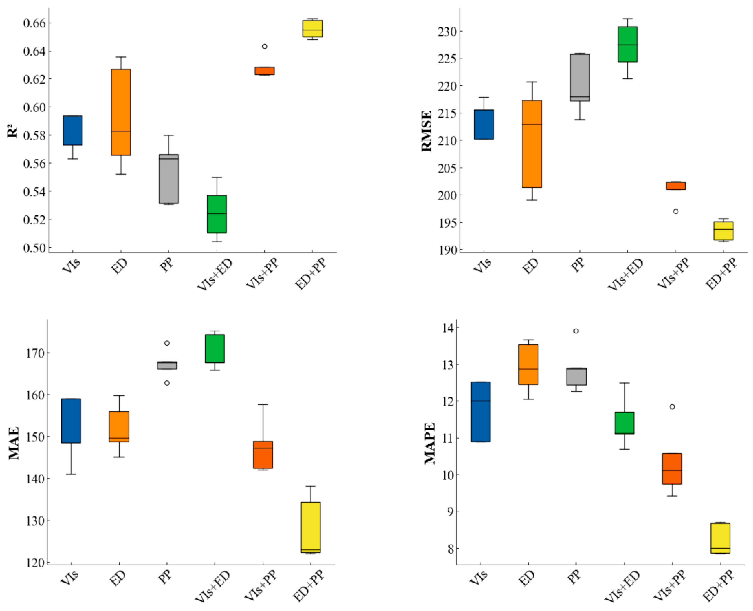
3.4. Analysis of Different Variables in Soybean Yield Prediction
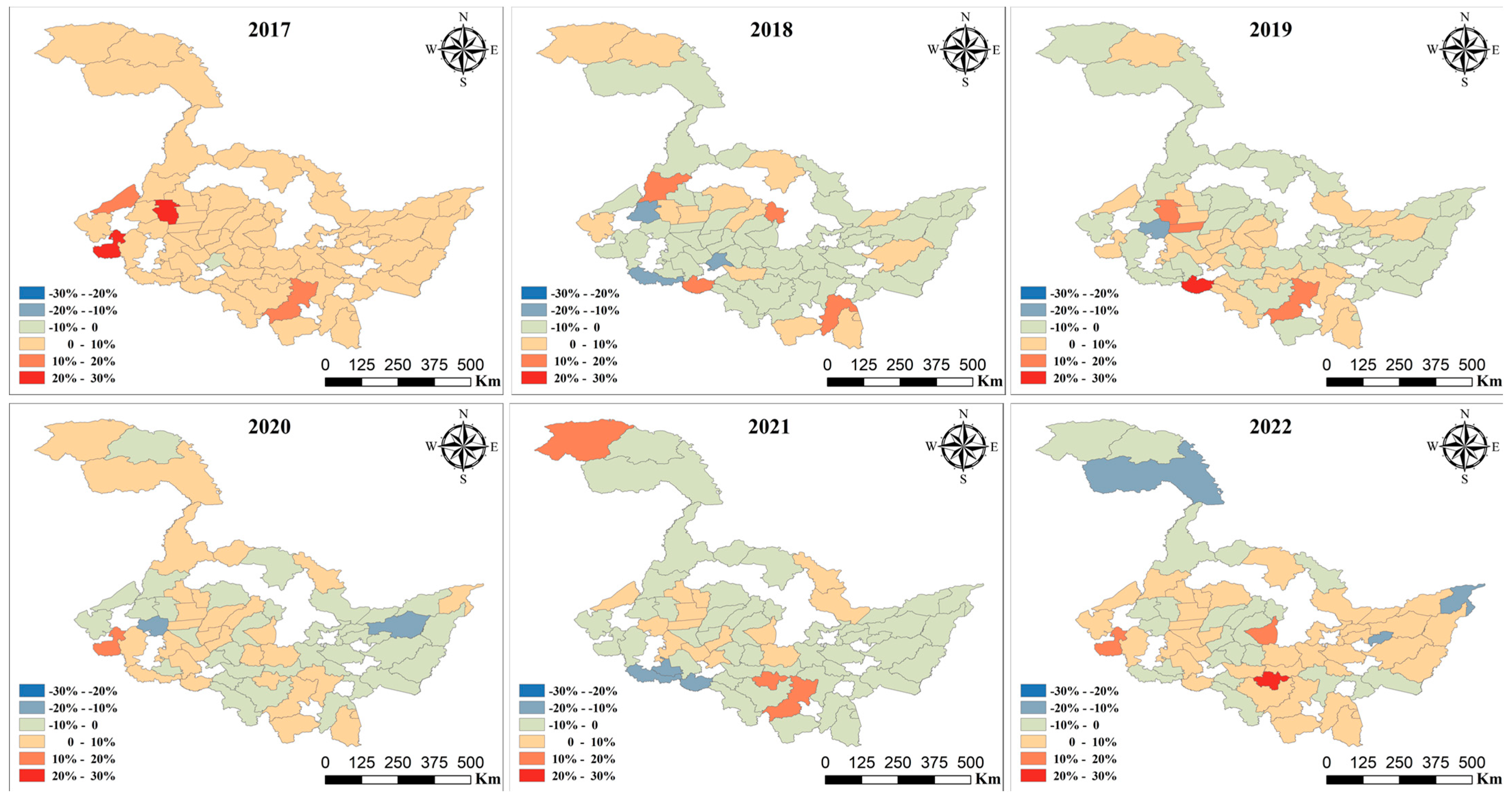
3.5. Spatial Distribution Map of Predicted Soybean Yield
4. Discussion
5. Conclusions
Author Contributions
Funding
Institutional Review Board Statement
Data Availability Statement
Conflicts of Interest
References
- Yu, H.; Li, J. Short-and long-term challenges in crop breeding. Natl. Sci. Rev. 2021, 8, nwab002. [Google Scholar] [CrossRef] [PubMed]
- Qin, P.; Wang, T.; Luo, Y. A review on plant-based proteins from soybean: Health benefits and soy product development. J. Agric. Food Res. 2022, 7, 100265. [Google Scholar] [CrossRef]
- Bazzana, D.; Foltz, J.; Zhang, Y. Impact of climate smart agriculture on food security: An agent-based analysis. Food Policy 2022, 111, 102304. [Google Scholar] [CrossRef]
- Wadas, W.; Kondraciuk, T. The Role of Foliar-Applied Silicon in Improving the Growth and Productivity of Early Potatoes. Agriculture 2025, 15, 556. [Google Scholar] [CrossRef]
- Yu, N.; Li, L.; Schmitz, N.; Tian, L.F.; Greenberg, J.A.; Diers, B.W. Development of methods to improve soybean yield estimation and predict plant maturity with an unmanned aerial vehicle based platform. Remote Sens. Environ. 2016, 187, 91–101. [Google Scholar] [CrossRef]
- Zhou, H.; Huang, F.; Lou, W.; Gu, Q.; Ye, Z.; Hu, H.; Zhang, X. Yield prediction through UAV-based multispectral imaging and deep learning in rice breeding trials. Agric. Syst. 2025, 223, 104214. [Google Scholar] [CrossRef]
- Okupska, E.; Gozdowski, D.; Pudełko, R.; Wójcik-Gront, E. Cereal and Rapeseed Yield Forecast in Poland at Regional Level Using Machine Learning and Classical Statistical Models. Agriculture 2025, 15, 984. [Google Scholar] [CrossRef]
- Li, Y.; Guan, K.; Yu, A.; Peng, B.; Zhao, L.; Li, B.; Peng, J. Toward building a transparent statistical model for improving crop yield prediction: Modeling rainfed corn in the U.S. Field Crops Res. 2019, 234, 55–65. [Google Scholar] [CrossRef]
- Keating, B.A.; Thorburn, P.J. Modelling crops and cropping systems—Evolving purpose, practice and prospects. Eur. J. Agron. 2018, 100, 163–176. [Google Scholar] [CrossRef]
- Osinga, S.A.; Paudel, D.; Mouzakitis, S.A.; Athanasiadis, I.N. Big data in agriculture: Between opportunity and solution. Agric. Syst. 2022, 195, 103298. [Google Scholar] [CrossRef]
- Feng, H.; Fan, Y.; Yue, J.; Bian, M.; Liu, Y.; Chen, R.; Ma, Y.; Fan, J.; Yang, G.; Zhao, C. Estimation of potato above-ground biomass based on the VGC-AGB model and deep learning. Comput. Electron. Agric. 2025, 232, 110122. [Google Scholar] [CrossRef]
- Wei, S.; Zhang, H.; Ling, J. A review of mangrove degradation assessment using remote sensing: Advances, challenges, and opportunities. GISci. Remote Sens. 2025, 62, 2491920. [Google Scholar] [CrossRef]
- Triantakonstantis, D.; Karakostas, A. Soil Organic Carbon Monitoring and Modelling via Machine Learning Methods Using Soil and Remote Sensing Data. Agriculture 2025, 15, 910. [Google Scholar] [CrossRef]
- Bregaglio, S.; Ginaldi, F.; Raparelli, E.; Fila, G.; Bajocco, S. Improving crop yield prediction accuracy by embedding phenological heterogeneity into model parameter sets. Agric. Syst. 2023, 209, 103666. [Google Scholar] [CrossRef]
- Arshad, S.; Kazmi, J.H.; Javed, M.G.; Mohammed, S. Applicability of machine learning techniques in predicting wheat yield based on remote sensing and climate data in Pakistan, South Asia. Eur. J. Agron. 2023, 147, 126837. [Google Scholar] [CrossRef]
- Lu, C.; Leng, G.; Liao, X.; Tu, H.; Qiu, J.; Li, J.; Huang, S.; Peng, J. In-season maize yield prediction in Northeast China: The phase-dependent benefits of assimilating climate forecast and satellite observations. Agric. For. Meteorol. 2024, 358, 110242. [Google Scholar] [CrossRef]
- Li, Y.; Liu, X.; Zhang, X.; Gu, X.; Yu, L.; Cai, H.; Peng, X. Using solar-induced chlorophyll fluorescence to predict winter wheat actual evapotranspiration through machine learning and deep learning methods. Agric. Water Manag. 2025, 309, 109322. [Google Scholar] [CrossRef]
- Zhu, H.; Lin, C.; Dong, Z.; Xu, J.-L.; He, Y. Early Yield Prediction of Oilseed Rape Using UAV-Based Hyperspectral Imaging Combined with Machine Learning Algorithms. Agriculture 2025, 15, 1100. [Google Scholar] [CrossRef]
- Lu, J.; Li, J.; Fu, H.; Tang, X.; Liu, Z.; Chen, H.; Sun, Y.; Ning, X. Deep Learning for Multi-Source Data-Driven Crop Yield Prediction in Northeast China. Agriculture 2024, 14, 794. [Google Scholar] [CrossRef]
- Khan, S.N.; Li, D.; Maimaitijiang, M. Using gross primary production data and deep transfer learning for crop yield prediction in the US Corn Belt. Int. J. Appl. Earth Obs. Geoinf. 2024, 131, 103965. [Google Scholar] [CrossRef]
- Du, J.; Zhang, Y.; Wang, P.; Tansey, K.; Liu, J.; Zhang, S. Enhancing Winter Wheat Yield Estimation With a CNN-Transformer Hybrid Framework Utilizing Multiple Remotely Sensed Parameters. IEEE Trans. Geosci. Remote Sens. 2025, 63, 4405213. [Google Scholar] [CrossRef]
- Lu, J.; Li, J.; Fu, H.; Zou, W.; Kang, J.; Yu, H.; Lin, X. Estimation of rice yield using multi-source remote sensing data combined with crop growth model and deep learning algorithm. Agric. For. Meteorol. 2025, 370, 110600. [Google Scholar] [CrossRef]
- Lu, J.; Fu, H.; Tang, X.; Liu, Z.; Huang, J.; Zou, W.; Chen, H.; Sun, Y.; Ning, X.; Li, J. GOA-optimized deep learning for soybean yield estimation using multi-source remote sensing data. Sci. Rep. 2024, 14, 7097. [Google Scholar] [CrossRef]
- Michael, N.E.; Bansal, R.C.; Ismail, A.A.A.; Elnady, A.; Hasan, S. A cohesive structure of Bi-directional long-short-term memory (BiLSTM) -GRU for predicting hourly solar radiation. Renew. Energy 2024, 222, 119943. [Google Scholar] [CrossRef]
- Ahmed, S.F.; Alam, M.S.B.; Hassan, M.; Rozbu, M.R.; Ishtiak, T.; Rafa, N.; Mofijur, M.; Shawkat Ali, A.B.M.; Gandomi, A.H. Deep learning modelling techniques: Current progress, applications, advantages, and challenges. Artif. Intell. Rev. 2023, 56, 13521–13617. [Google Scholar] [CrossRef]
- Hu, Z.; Chen, L.; Luo, Y.; Zhou, J. EEG-Based Emotion Recognition Using Convolutional Recurrent Neural Network with Multi-Head Self-Attention. Appl. Sci. 2022, 12, 11255. [Google Scholar] [CrossRef]
- Liu, T.; Yu, L.; Bu, K.; Yan, F.; Zhang, S. Seasonal local temperature responses to paddy field expansion from rain-fed farmland in the cold and humid Sanjiang Plain of China. Remote Sens. 2018, 10, 2009. [Google Scholar] [CrossRef]
- Ma, H.; Wang, C.; Liu, J.; Yuan, Z.; Yao, C.; Wang, X.; Pan, X. Separate prediction of soil organic matter in drylands and paddy fields based on optimal image synthesis method in the Sanjiang Plain, Northeast China. Geoderma 2024, 447, 116929. [Google Scholar] [CrossRef]
- Wang, W.; Deng, X.; Yue, H. Black soil conservation will boost China’s grain supply and reduce agricultural greenhouse gas emissions in the future. Environ. Impact Assess. Rev. 2024, 106, 107482. [Google Scholar] [CrossRef]
- Xin, M.; Zhang, Z.; Han, Y.; Feng, L.; Lei, Y.; Li, X.; Wu, F.; Wang, J.; Wang, Z.; Li, Y. Soybean phenological changes in response to climate warming in three northeastern provinces of China. Field Crops Res. 2023, 302, 109082. [Google Scholar] [CrossRef]
- Wang, T.; Ma, Y.; Luo, S. Spatiotemporal Evolution and Influencing Factors of Soybean Production in Heilongjiang Province, China. Land 2023, 12, 2090. [Google Scholar] [CrossRef]
- Jasinski, M.F. Sensitivity of the normalized difference vegetation index to subpixel canopy cover, soil albedo, and pixel scale. Remote Sens. Environ. 1990, 32, 169–187. [Google Scholar] [CrossRef]
- Huete, A.R.; Liu, H.Q.; Batchily, K.V.; Van Leeuwen, W. A comparison of vegetation indices over a global set of TM images for EOS-MODIS. Remote Sens. Environ. 1997, 59, 440–451. [Google Scholar] [CrossRef]
- McFeeters, S.K. The use of the Normalized Difference Water Index (NDWI) in the delineation of open water features. Int. J. Remote Sens. 1996, 17, 1425–1432. [Google Scholar] [CrossRef]
- Nendel, C.; Reckling, M.; Debaeke, P.; Schulz, S.; Berg-Mohnicke, M.; Constantin, J.; Fronzek, S.; Hoffmann, M.; Jakšić, S.; Kersebaum, K.-C.; et al. Future area expansion outweighs increasing drought risk for soybean in Europe. Glob. Change Biol. 2023, 29, 1340–1358. [Google Scholar] [CrossRef]
- Zhang, H.; Zhao, Y.; Zhu, J.-K. Thriving under Stress: How Plants Balance Growth and the Stress Response. Dev. Cell 2020, 55, 529–543. [Google Scholar] [CrossRef] [PubMed]
- Sato, H.; Mizoi, J.; Shinozaki, K.; Yamaguchi-Shinozaki, K. Complex plant responses to drought and heat stress under climate change. Plant J. 2024, 117, 1873–1892. [Google Scholar] [CrossRef]
- Yang, A.; Luo, S.; Xu, Y.; Zhang, P.; Sun, Z.; Hu, K.; Li, M. Optimization of Irrigation and Fertilization in Maize-Soybean System Based on Coupled Water-Carbon-Nitrogen Interactions. Agronomy 2025, 15, 41. [Google Scholar] [CrossRef]
- Williams, M.; Rastetter, E.B.; Fernandes, D.N.; Goulden, M.L.; Shaver, G.R.; Johnson, L.C. Predicting gross primary productivity in terrestrial ecosystems. Ecol. Appl. 1997, 7, 882–894. [Google Scholar] [CrossRef]
- Peltier, G.; Stoffel, C.; Findinier, J.; Madireddi, S.K.; Dao, O.; Epting, V.; Morin, A.; Grossman, A.; Li-Beisson, Y.; Burlacot, A. Alternative electron pathways of photosynthesis power green algal CO2 capture. Plant Cell 2024, 36, 4132–4142. [Google Scholar] [CrossRef]
- Pinker, R.T.; Laszlo, I. Global distribution of photosynthetically active radiation as observed from satellites. J. Clim. 1992, 5, 56–65. [Google Scholar] [CrossRef]
- Fang, H.; Baret, F.; Plummer, S.; Schaepman-Strub, G. An overview of global leaf area index (LAI): Methods, products, validation, and applications. Rev. Geophys. 2019, 57, 739–799. [Google Scholar] [CrossRef]
- Duan, J.; Wang, H.; Yang, Y.; Cheng, M.; Li, D. Rice Growth Parameter Estimation Based on Remote Satellite and Unmanned Aerial Vehicle Image Fusion. Agriculture 2025, 15, 26. [Google Scholar] [CrossRef]
- Dou, J.; Yunus, A.P.; Tien Bui, D.; Merghadi, A.; Sahana, M.; Zhu, Z.; Chen, C.-W.; Khosravi, K.; Yang, Y.; Pham, B.T. Assessment of advanced random forest and decision tree algorithms for modeling rainfall-induced landslide susceptibility in the Izu-Oshima Volcanic Island, Japan. Sci. Total Environ. 2019, 662, 332–346. [Google Scholar] [CrossRef]
- Zhang, F.; Deb, C.; Lee, S.E.; Yang, J.; Shah, K.W. Time series forecasting for building energy consumption using weighted Support Vector Regression with differential evolution optimization technique. Energy Build. 2016, 126, 94–103. [Google Scholar] [CrossRef]
- Li, Q.-F.; Song, Z.-M. High-performance concrete strength prediction based on ensemble learning. Constr. Build. Mater. 2022, 324, 126694. [Google Scholar] [CrossRef]
- Dai, G.; Tian, Z.; Fan, J.; Sunil, C.K.; Dewi, C. DFN-PSAN: Multi-level deep information feature fusion extraction network for interpretable plant disease classification. Comput. Electron. Agric. 2024, 216, 108481. [Google Scholar] [CrossRef]
- Shin, H.-C.; Roth, H.R.; Gao, M.; Lu, L.; Xu, Z.; Nogues, I.; Yao, J.; Mollura, D.; Summers, R.M. Deep convolutional neural networks for computer-aided detection: CNN architectures, dataset characteristics and transfer learning. IEEE Trans. Med. Imaging 2016, 35, 1285–1298. [Google Scholar] [CrossRef] [PubMed]
- Shi, Z.; Ye, Y.; Wu, Y. Rank-based pooling for deep convolutional neural networks. Neural Netw. 2016, 83, 21–31. [Google Scholar] [CrossRef]
- Awadallah, M.A.; Makhadmeh, S.N.; Al-Betar, M.A.; Dalbah, L.M.; Al-Redhaei, A.; Kouka, S.; Enshassi, O.S. Multi-objective ant colony optimization: Review. Arch. Comput. Methods Eng. 2025, 32, 995–1037. [Google Scholar] [CrossRef]
- Chen, J.; Jing, H.; Chang, Y.; Liu, Q. Gated recurrent unit based recurrent neural network for remaining useful life prediction of nonlinear deterioration process. Reliab. Eng. Syst. Saf. 2019, 185, 372–382. [Google Scholar] [CrossRef]
- Tan, T.H.; Chang, Y.L.; Wu, J.R.; Chen, Y.F.; Alkhaleefah, M. Convolutional Neural Network with Multihead Attention for Human Activity Recognition. IEEE Internet Things J. 2024, 11, 3032–3043. [Google Scholar] [CrossRef]
- Liu, D.; Dong, X.; Bian, D.; Zhou, W. Epileptic Seizure Prediction Using Attention Augmented Convolutional Network. Int. J. Neural Syst. 2023, 33, 2350054. [Google Scholar] [CrossRef] [PubMed]
- Gueymard, C.A. A review of validation methodologies and statistical performance indicators for modeled solar radiation data: Towards a better bankability of solar projects. Renew. Sustain. Energy Rev. 2014, 39, 1024–1034. [Google Scholar] [CrossRef]
- Syed, T.N.; Zhou, J.; Lakhiar, I.A.; Marinello, F.; Gemechu, T.T.; Rottok, L.T.; Jiang, Z. Enhancing Autonomous Orchard Navigation: A Real-Time Convolutional Neural Network-Based Obstacle Classification System for Distinguishing ‘Real’ and ‘Fake’ Obstacles in Agricultural Robotics. Agriculture 2025, 15, 827. [Google Scholar] [CrossRef]
- Wang, J.; Wang, P.; Tian, H.; Tansey, K.; Liu, J.; Quan, W. A deep learning framework combining CNN and GRU for improving wheat yield estimates using time series remotely sensed multi-variables. Comput. Electron. Agric. 2023, 206, 107705. [Google Scholar] [CrossRef]
- Shi, S.; Xu, L.; Gong, W.; Chen, B.; Chen, B.; Qu, F.; Tang, X.; Sun, J.; Yang, J. A convolution neural network for forest leaf chlorophyll and carotenoid estimation using hyperspectral reflectance. Int. J. Appl. Earth Obs. Geoinf. 2022, 108, 102719. [Google Scholar] [CrossRef]
- Xia, Y.; Ding, D.; Chang, Z.; Li, F. Joint Deep Networks Based Multi-Source Feature Learning for QoS Prediction. IEEE Trans. Serv. Comput. 2022, 15, 2314–2327. [Google Scholar] [CrossRef]
- Wang, M.; Li, T. Correction: Wang, M.; Li, T. Pest and Disease Prediction and Management for Sugarcane Using a Hybrid Autoregressive Integrated Moving Average—A Long Short-Term Memory Model. Agriculture 2025, 15, 500. Agriculture 2025, 15, 774. [Google Scholar] [CrossRef]
- Radočaj, D.; Jurišić, M. A Phenology-Based Evaluation of the Optimal Proxy for Cropland Suitability Based on Crop Yield Correlations from Sentinel-2 Image Time-Series. Agriculture 2025, 15, 859. [Google Scholar] [CrossRef]
- Castro, J.C.; Dohleman, F.G.; Bernacchi, C.J.; Long, S.P. Elevated CO2 significantly delays reproductive development of soybean under Free-Air Concentration Enrichment (FACE). J. Exp. Bot. 2009, 60, 2945–2951. [Google Scholar] [CrossRef] [PubMed]
- Gitelson, A.; Viña, A.; Solovchenko, A.; Arkebauer, T.; Inoue, Y. Derivation of canopy light absorption coefficient from reflectance spectra. Remote Sens. Environ. 2019, 231, 111276. [Google Scholar] [CrossRef]
- von Bloh, M.; Nóia Júnior, R.d.S.; Wangerpohl, X.; Saltık, A.O.; Haller, V.; Kaiser, L.; Asseng, S. Machine learning for soybean yield forecasting in Brazil. Agric. For. Meteorol. 2023, 341, 109670. [Google Scholar] [CrossRef]
- Shen, L.; Li, Z.; Hao, J.; Wang, L.; Chen, H.; Wang, Y.; Xia, B. Evaluating the Dynamic Response of Cultivated Land Expansion and Fallow Urgency in Arid Regions Using Remote Sensing and Multi-Source Data Fusion Methods. Agriculture 2025, 15, 839. [Google Scholar] [CrossRef]
- Clarke, B.; Otto, F.; Stuart-Smith, R.; Harrington, L. Extreme weather impacts of climate change: An attribution perspective. Environ. Res. Clim. 2022, 1, 012001. [Google Scholar] [CrossRef]
- Song, X.-P.; Li, H.; Potapov, P.; Hansen, M.C. Annual 30 m soybean yield mapping in Brazil using long-term satellite observations, climate data and machine learning. Agric. For. Meteorol. 2022, 326, 109186. [Google Scholar] [CrossRef]
- He, M.; Li, H.; Sun, Z.; Li, X.; Li, Q.; Cai, J.; Zhou, Q.; Zhong, Y.; Wang, X.; Jiang, D. Drought priming enhances young spike development in wheat under drought stress during stem elongation. J. Integr. Agric. 2025; in press. [Google Scholar] [CrossRef]
- Huang, J.; Tian, L.; Liang, S.; Ma, H.; Becker-Reshef, I.; Huang, Y.; Su, W.; Zhang, X.; Zhu, D.; Wu, W. Improving winter wheat yield estimation by assimilation of the leaf area index from Landsat TM and MODIS data into the WOFOST model. Agric. For. Meteorol. 2015, 204, 106–121. [Google Scholar] [CrossRef]
- Croce, R.; Carmo-Silva, E.; Cho, Y.B.; Ermakova, M.; Harbinson, J.; Lawson, T.; McCormick, A.J.; Niyogi, K.K.; Ort, D.R.; Patel-Tupper, D.; et al. Perspectives on improving photosynthesis to increase crop yield. Plant Cell 2024, 36, 3944–3973. [Google Scholar] [CrossRef]
- Mohammadi, S.; Rydgren, K.; Bakkestuen, V.; Gillespie, M.A.K. Impacts of recent climate change on crop yield can depend on local conditions in climatically diverse regions of Norway. Sci. Rep. 2023, 13, 3633. [Google Scholar] [CrossRef]
- Devkota, K.P.; Bouasria, A.; Devkota, M.; Nangia, V. Predicting wheat yield gap and its determinants combining remote sensing, machine learning, and survey approaches in rainfed Mediterranean regions of Morocco. Eur. J. Agron. 2024, 158, 127195. [Google Scholar] [CrossRef]
- Burroughs, C.H.; Montes, C.M.; Moller, C.A.; Mitchell, N.G.; Michael, A.M.; Peng, B.; Kimm, H.; Pederson, T.L.; Lipka, A.E.; Bernacchi, C.J.; et al. Reductions in leaf area index, pod production, seed size, and harvest index drive yield loss to high temperatures in soybean. J. Exp. Bot. 2023, 74, 1629–1641. [Google Scholar] [CrossRef] [PubMed]
- Wu, P.; Wang, Y.; Shao, J.; Yu, H.; Zhao, Z.; Li, L.; Gao, P.; Li, Y.; Liu, S.; Gao, C.; et al. Enhancing productivity while reducing water footprint and groundwater depletion: Optimizing irrigation strategies in a wheat-soybean planting system. Field Crops Res. 2024, 309, 109331. [Google Scholar] [CrossRef]


| Data | Variable | Temporal Resolution | Spatial Resolution | Source |
|---|---|---|---|---|
| Vegetation indices | NDVI, EVI, NDWI, RVI, GNDVI | 16 days | 500 m | MOD13A1 |
| Environmental data | PR, AET, PDSI, DEF, SRAD, TMMN, TMMX, VPD, VAP | Monthly | 1 km | TerraClimate datasets |
| Photosynthetically active indices | Gpp, PsnNet, Fpar, Lai | Monthly | 500 m | MODIS |
| Soybean yield and planting area | Planting area | Year | 30 m | https://doi.org/10.5194/essd-12-3081-2020 (accessed on 23 June 2024) |
| Yield data for soybean | Year | City | https://tjj.hlj.gov.cn/ (accessed on 23 June 2024) |
| Vegetation Index | Description | Formula |
|---|---|---|
| NDVI | Normalized difference vegetation index | |
| EVI | Enhanced vegetation index | |
| NDWI | Normalized difference water index | |
| RVI | Ratio vegetation index | |
| GNDVI | Green normalized difference vegetation index | |
| GVCI | Green vegetation canopy index | |
| SAVI | Soil adjusted vegetation index | |
| WDRVI | Wide-dynamic-range vegetation index | |
| GLI | Green leaf index | |
| CVI | Chlorophyll vegetation index |
| Model | R2 | RMSE (kg/ha) | MAE (kg/ha) | MAPE (%) | |
|---|---|---|---|---|---|
| 2021 | RFR | 0.41 ± 0.10 | 142.66 ± 25.58 | 113.75 ± 16.98 | 6.35 ± 1.27 |
| SVR | 0.43 ± 0.05 | 207.68 ± 33.57 | 171.92 ± 38.74 | 11.07 ± 2.70 | |
| XGBoost | 0.39 ± 0.04 | 202.57 ± 34.37 | 161.95 ± 22.15 | 10.13 ± 2.47 | |
| CNN | 0.64 ± 0.02 | 198.13 ± 4.94 | 150.17 ± 4.19 | 12.81 ± 0.36 | |
| ACGM | 0.75 ± 0.02 | 163.18 ± 5.02 | 127.83 ± 8.98 | 9.19 ± 0.79 | |
| 2022 | RFR | 0.42 ± 0.08 | 198.34 ± 32.04 | 160.54 ± 21.81 | 10.43 ± 2.21 |
| SVR | 0.49 ± 0.05 | 133.09 ± 30.95 | 107.26 ± 25.04 | 5.96 ± 1.78 | |
| XGBoost | 0.36 ± 0.03 | 153.30 ± 19.33 | 119.50 ± 13.28 | 6.51 ± 0.82 | |
| CNN | 0.66 ± 0.02 | 143.27 ± 4.79 | 115.69 ± 5.07 | 6.57 ± 0.39 | |
| ACGM | 0.74 ± 0.02 | 123.94 ± 4.78 | 105.39 ± 3.95 | 6.21 ± 0.30 |
Disclaimer/Publisher’s Note: The statements, opinions and data contained in all publications are solely those of the individual author(s) and contributor(s) and not of MDPI and/or the editor(s). MDPI and/or the editor(s) disclaim responsibility for any injury to people or property resulting from any ideas, methods, instructions or products referred to in the content. |
© 2025 by the authors. Licensee MDPI, Basel, Switzerland. This article is an open access article distributed under the terms and conditions of the Creative Commons Attribution (CC BY) license (https://creativecommons.org/licenses/by/4.0/).
Share and Cite
Fu, H.; Li, J.; Lu, J.; Lin, X.; Kang, J.; Zou, W.; Ning, X.; Sun, Y. Prediction of Soybean Yield at the County Scale Based on Multi-Source Remote-Sensing Data and Deep Learning Models. Agriculture 2025, 15, 1337. https://doi.org/10.3390/agriculture15131337
Fu H, Li J, Lu J, Lin X, Kang J, Zou W, Ning X, Sun Y. Prediction of Soybean Yield at the County Scale Based on Multi-Source Remote-Sensing Data and Deep Learning Models. Agriculture. 2025; 15(13):1337. https://doi.org/10.3390/agriculture15131337
Chicago/Turabian StyleFu, Hongkun, Jian Li, Jian Lu, Xinglei Lin, Junrui Kang, Wenlong Zou, Xiangyu Ning, and Yue Sun. 2025. "Prediction of Soybean Yield at the County Scale Based on Multi-Source Remote-Sensing Data and Deep Learning Models" Agriculture 15, no. 13: 1337. https://doi.org/10.3390/agriculture15131337
APA StyleFu, H., Li, J., Lu, J., Lin, X., Kang, J., Zou, W., Ning, X., & Sun, Y. (2025). Prediction of Soybean Yield at the County Scale Based on Multi-Source Remote-Sensing Data and Deep Learning Models. Agriculture, 15(13), 1337. https://doi.org/10.3390/agriculture15131337