Integrating Geodetector and GTWR to Unveil Spatiotemporal Heterogeneity in China’s Agricultural Carbon Emissions Under the Dual Carbon Goals

Abstract

Against the backdrop of intensifying global climate change and deepening sustainable development goals, the low-carbon transformation of agriculture, as a major greenhouse gas emission source, holds significant strategic importance for achieving China’s “carbon peaking and carbon neutrality” (referred to as the “dual carbon”) targets. To reveal the spatiotemporal evolution characteristics and complex driving mechanisms of agricultural carbon emissions (ACEs), this study constructs a comprehensive accounting framework for agricultural carbon emissions based on provincial panel data from China spanning 2000 to 2023. The framework encompasses three major carbon sources—cropland use, rice cultivation, and livestock farming—enabling precise quantification of total agricultural carbon emissions. Furthermore, spatial-temporal distribution patterns are characterized using methodologies including standard deviational ellipse (SDE) and spatial autocorrelation analysis. For driving mechanism identification, the Geodetector and Geographically and Temporally Weighted Regression (GTWR) models are employed. The former quantifies the spatial explanatory power and interaction effects of driving factors, while the latter enables dynamic estimation of factor influence intensities across temporal and spatial dimensions, jointly revealing significant spatiotemporal heterogeneity in driving mechanisms. Key findings: (1) temporally, total ACEs exhibit fluctuating growth, while emission intensity has significantly decreased, indicating the combined effects of policy regulation and technological advancements; (2) spatially, emissions display an “east-high, west-low” pattern, with an increasing number of hotspot areas and a continuous shift of the emission centroid toward the northwest; and (3) mechanistically, agricultural gross output value is the primary driving factor, with its influence fluctuating in response to economic and policy changes. The interactions among multiple factors evolve over time, transitioning from economy-driven to synergistic effects of technology and climate. The GTWR model further reveals the spatial and temporal variations in the impacts of each factor. This study recommends formulating differentiated low-carbon agricultural policies based on regional characteristics, optimizing industrial structures, enhancing modernization levels, strengthening regional collaborative governance, and promoting the synergistic development of climate and agriculture. These measures provide a scientific basis and policy reference for achieving the “dual carbon” goals.

1. Introduction

Carbon emissions serve as the core driver of global warming, whose persistent accumulation has triggered a series of environmental crises, including frequent extreme climate events, accelerated glacial melting, and biodiversity decline, posing profound threats to both human society and natural ecosystems [1,2]. Within the global carbon emission structure, ACEs hold significant prominence, primarily originating from activities such as farmland soil management, fertilizer/pesticide application, livestock enteric fermentation, and agricultural energy consumption. These processes not only directly increase greenhouse gas concentrations, but also indirectly exacerbate ecological pressures through land degradation and resource overuse [3]. As the world’s second-largest economy and agricultural powerhouse, China proposed the “dual carbon” targets in 2020, explicitly incorporating the agricultural sector as a pivotal component in the low-carbon transition [4]. However, while ensuring food security, China’s agricultural production has experienced a notable increase in carbon emissions, with total agricultural greenhouse gas emissions reaching 12.999 billion metric tons CO₂ equivalent (CO₂-eq) in 2020, accounting for 24.62% of global emissions [5]. The complexity of its spatiotemporal distribution patterns and driving mechanisms demands urgent elucidation [6]. Therefore, under the “dual carbon” strategic framework, in-depth investigation into the spatiotemporal evolution of China’s ACEs and its influencing factors will not only facilitate the identification of mitigation potentials and optimization pathways, but also carry crucial theoretical and practical significance for advancing national green development and global climate governance.

Based on this, this study will first construct an agricultural carbon emission measurement model incorporating three major carbon sources—farmland utilization, rice cultivation, and livestock breeding—to calculate and decompose province-level ACEs in China. Subsequently, employing methods such as standard deviation ellipse and spatial autocorrelation analysis, we aim to reveal the spatiotemporal evolution patterns of ACE in China. Finally, through the integrated application of Geodetector and GTWR models, we systematically investigate the spatiotemporal evolution patterns and heterogeneous characteristics of influencing factors on ACEs in China. Notably, as one of the world’s largest agricultural producers, China’s ACEs exhibit unique and representative characteristics: its vast agricultural scale, diversified production structure, and rapidly advancing modernization process render both its emission patterns and mitigation practices globally significant for reference. This study seeks to address three core questions: How have the spatial patterns and temporal trends of China’s ACEs evolved? What are the key drivers behind these changes? Does the intensity of these factors’ effects vary according to regional characteristics and temporal phases? By elucidating these patterns, our research not only provides scientific support for low-carbon agricultural development under China’s “dual carbon” goals, but also offers replicable analytical frameworks and practical references for other developing countries confronting similar challenges.

2. Literature Review

Pioneering studies on ACE and spatiotemporal analysis have laid the foundation for this field. West and Marland [7] first proposed a framework for agricultural carbon flux accounting, analyzing the impact of farming practices on carbon emissions and sinks, providing a methodological cornerstone for global ACE accounting. Zhao and Qin [8] investigated spatiotemporal variation of carbon sources and sinks in farmland ecosystems in China’s coastal regions, proposing a preliminary regional carbon compensation mechanism. These studies highlighted the critical role of soil management and land use in emissions, establishing the theoretical starting point for ACE research. Major theoretical contributions have further enriched research perspectives. The IPCC inventory method has become the standard for regional emission estimation, combined with GIS technology to characterize spatial patterns. The STIRPAT model quantifies driving mechanisms such as economic, demographic, and technological factors, deepening the systemic understanding of emission sources.

ACE research has continued to advance in methodology and scale. In terms of spatiotemporal evolution, studies at provincial or regional scales have employed the IPCC inventory method to estimate total ACEs and used GIS techniques to reveal spatial distribution characteristics, laying the groundwork for driver analysis [9,10,11,12]. Tian et al. applied spatial autocorrelation analysis to reveal regional clustering of provincial ACEs in China, emphasizing the nonlinear effects of agricultural inputs [13]. Luo et al. used decoupling analysis to assess the relationship between ACEs and economic growth, uncovering regional emission reduction potential [14]. Panchasara et al. highlighted the regulatory role of climatic variables on emissions [15]. These advancements have promoted refined accounting and policy-oriented research.

In the domain of ACE spatiotemporal analysis, traditional econometric and spatial econometric models have quantified the contributions of factors such as agricultural land use [16,17], fertilizer application [18,19], agricultural mechanization levels [20,21], and livestock farming [22,23], providing insights into driving mechanisms. However, existing studies have limitations: (1) spatiotemporal evolution studies often focus on total emissions estimation and static spatial descriptions, neglecting the dynamic changes in emission patterns and their interactions with driving factors; and (2) traditional models assume uniform factor impacts across regions and time periods, overlooking the spatiotemporal heterogeneity of regional natural conditions, production practices, and policy environments.

This study addresses these gaps by coupling the Geodetector and GTWR models. Geodetector quantifies the relative importance of driving factors and their complex interactive effects [24,25], compensating for the inability of traditional methods to reveal synergistic relationships. GTWR incorporates the temporal dimension, dynamically estimating the intensity and direction of factor effects across different regions and time periods through localized regression, overcoming the limitations of global models that ignore spatiotemporal non-stationarity [26,27]. This coupled approach precisely captures the spatiotemporal heterogeneity of ACE, deepening the understanding of driving mechanisms and providing a scientific basis for differentiated and dynamic emission reduction strategies under the “dual carbon” goals. Additionally, both methods are computationally efficient, produce intuitive and interpretable results, and have no strict assumptions about data distribution, demonstrating significant applicability and superiority in analyzing complex agricultural systems [28].

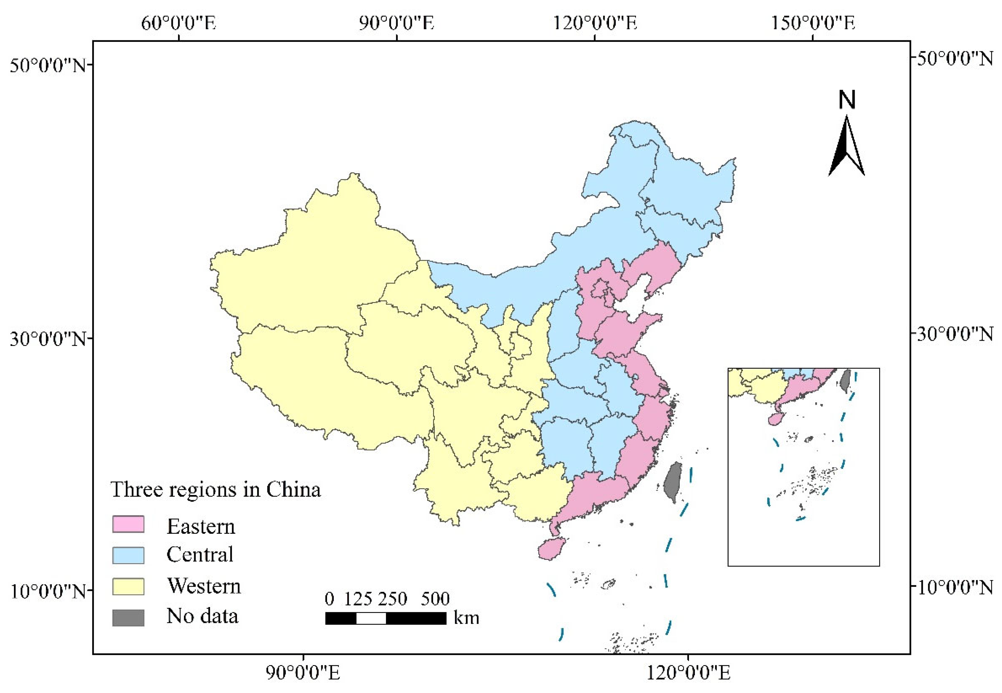
3. Overview of the Study Area

This study encompasses 31 provincial administrative regions in China, spanning from 73°33′ E to 135°05′ E longitude and 18°51′ N to 53°33′ N latitude (Figure 1). China’s topography exhibits a three-tiered ladder descending from west to east: western high-altitude plateaus and mountains transition to central basins and hills, culminating in eastern plains. Climatic zones range from cold-temperate to tropical, with annual precipitation decreasing northwestward from 2000 mm to less than 50 mm [29]. With a population exceeding 1.4 billion (as of 2023), approximately 25% of which is engaged in agriculture, China achieved a grain output of 687 million metric tons in 2022, securing its position as the world’s leading agricultural producer [30].

Agricultural production exhibits pronounced regional heterogeneity: eastern coastal regions specialize in staple crop cultivation with intensive fertilizer application and mechanization (73% mechanization rate in 2022); central China serves as the primary grain production base with intensive farming activities; and western areas focus on animal husbandry and specialty agriculture. ACEs reached approximately 830 million metric tons CO₂-eq in 2020, accounting for 7–10% of national emissions. Emission hotspots concentrate in eastern regions, while western areas show significant emissions from pastoral activities and land-use practices. Accelerated agricultural modernization, marked by a 73% mechanization rate (2022) coupled with substantial fertilizer application (51.9 million metric tons in 2022), has significantly influenced the spatiotemporal patterns of carbon emissions [31].

Under the “dual carbon” goals, China’s agricultural sector faces urgent demands for low-carbon transition. Policy-driven green transition initiatives are emerging, exemplified by the 2022 “Agricultural and Rural Emission Reduction and Carbon Sequestration Implementation Plan” specifying mitigation targets. Variations in regional natural conditions and production methods generate significant heterogeneity in emission mechanisms and mitigation potential across spatial domains [32]. Examining national-scale patterns enables the identification of spatiotemporal regularities, thereby informing tailored mitigation strategies, while simultaneously offering global reference value.

4. Research Methods and Data Sources

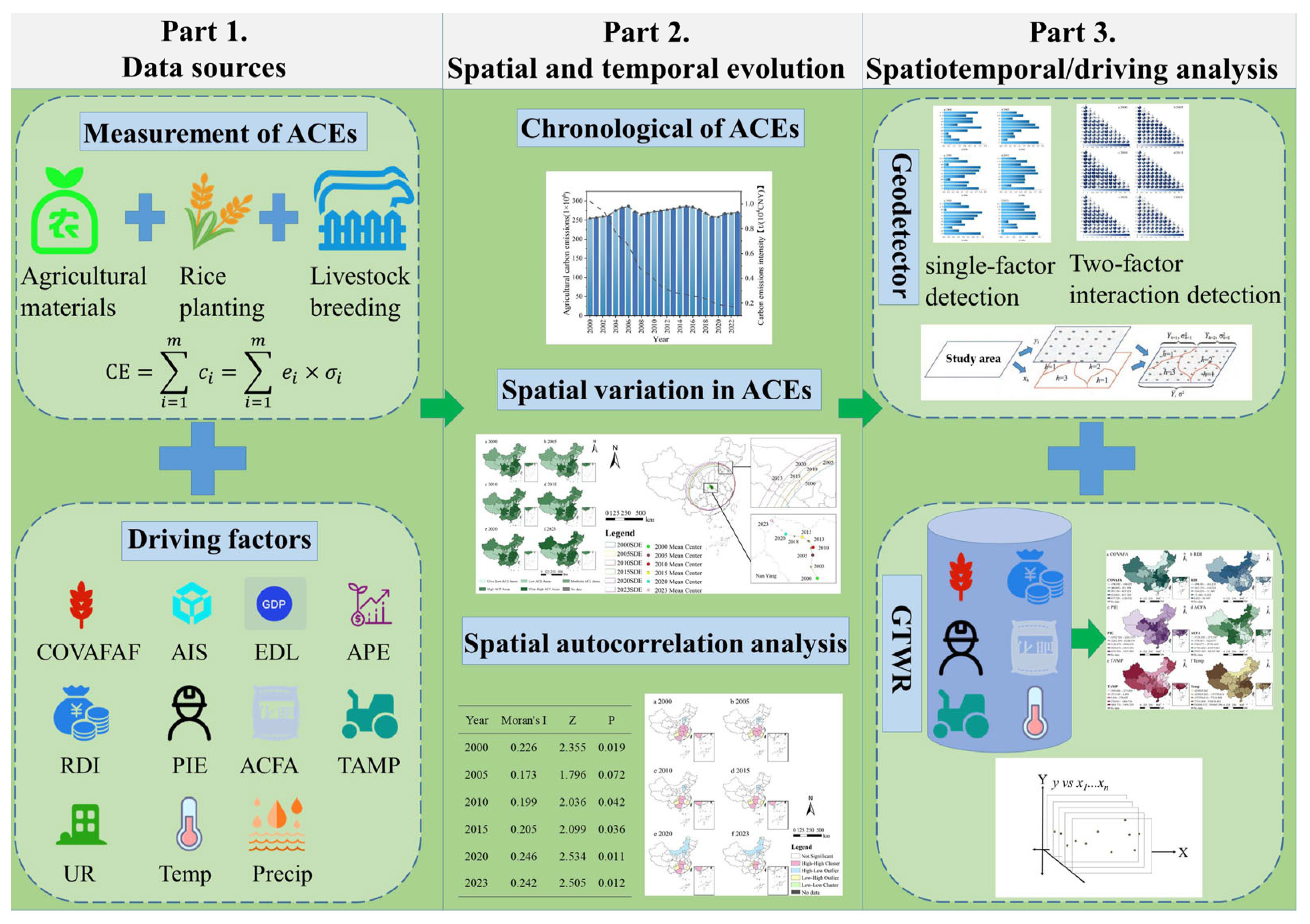
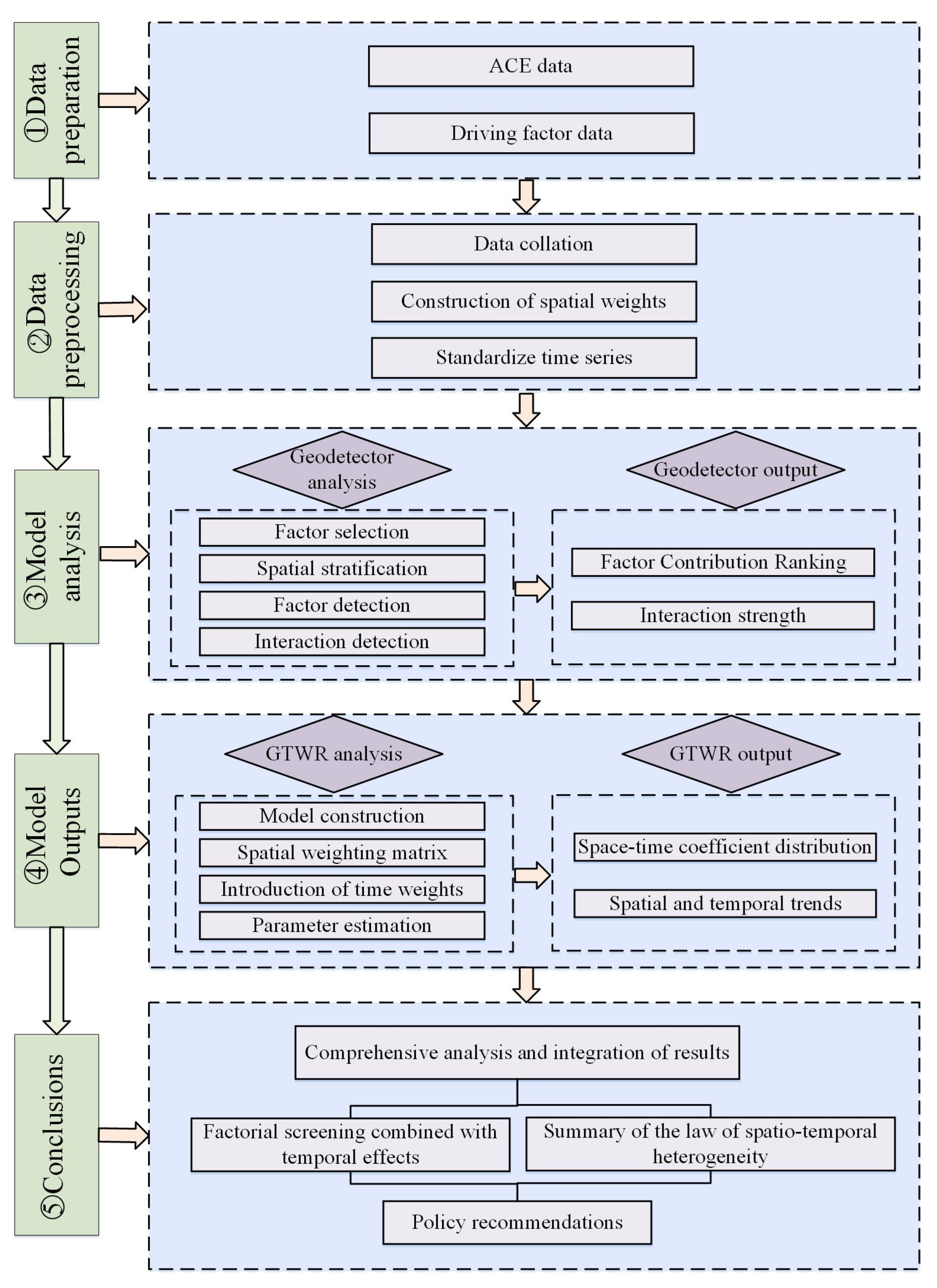
4.1. Research Framework

This study constructs a comprehensive analytical framework (Figure 2) to systematically investigate the spatiotemporal evolution patterns, key driving factors, and spatial heterogeneity characteristics of ACE. First, a carbon emission accounting method was established based on three primary carbon sources—agricultural land use, rice cultivation, and livestock farming—to accurately estimate provincial ACE totals. For identifying influencing factors, a multidimensional indicator system encompassing economic development, agricultural inputs, and climatic conditions was developed, laying the foundation for analyzing driving mechanisms. In the spatiotemporal evolution analysis, the standard deviational ellipse and centroid migration methods were employed to characterize the spatial distribution patterns of ACEs, while spatial autocorrelation analysis was used to verify their spatial clustering. Furthermore, to deeply explore the driving mechanisms, this study innovatively integrates the Geodetector model with the GTWR model, revealing the spatial heterogeneity impacts and mechanisms of various driving factors on ACEs from both global differentiation and local response perspectives.

4.2. ACE Accounting

This study employs established methodologies to quantify ACE through three primary pathways: agricultural land use, rice cultivation, and livestock husbandry. The computational framework is expressed as [33]

$$CE={\displaystyle {\sum }_{i=1}^m{C}_i}={\displaystyle {\sum }_{i=1}^m{e}_i}\times {\sigma }_i$$

(1)

where CE denotes total ACEs (10⁶ tons), C_i indicates emissions from the i-th source (10⁶ tons), and e_i represents the activity level of the i-th source and corresponds to the emission factor for the i-th source. The calculation adopts the methodological framework developed by Tian et al. [34] for cropland emissions, encompassing six distinct emission sources: chemical fertilizers, pesticides, plastic sheeting, diesel oil, ploughing, and irrigation systems.

The following are the explicit definitions of key variables for the three categories of carbon sources, along with the specific activities and processes involved:

Agricultural land use: Refers to agricultural production activities on arable land that directly or indirectly generate carbon emissions. Specific activities include the application of chemical fertilizers, pesticide spraying, use of plastic mulching (for insulation or weed control), diesel-powered farm machinery operation, mechanical tillage, and irrigation pumping.

Rice cultivation: Refers to methane (CH₄) emissions generated from the anaerobic environment of flooded paddy fields during the rice growth cycle. Activities encompass the cultivation processes of early rice, late rice, and single-season rice, including seedling preparation, transplanting, field management, and harvesting, with a focus on the contribution of flood management to CH₄ emissions.

Livestock farming: Refers to CH₄ and nitrous oxide (N₂O) emissions produced during livestock rearing, involving cattle, horses, donkeys, mules, pigs, goats, and sheep. Specific activities include enteric fermentation in livestock (release of CH₄ during digestion) and manure management (release of CH₄ and N₂O during composting, storage, and treatment processes).

The corresponding emission factors for each carbon source are detailed in

Table 1. The carbon emission coefficient of major agricultural sources.

Carbon Sources	Carbon Emission Coefficient	Reference Source
Fertilizers	0.8956 kg C kg−1	[33]
Pesticides	4.9341 kg C kg−1	[33]
Plastic sheeting	5.18 kg C kg−1	[13]
Diesel oil	0.5927 kg C kg−1	IPCC [35]
Plough	312.6kg·km−2	[36]
Irrigation	266.48 kg C kg−1	[33]

.

As a critical greenhouse gas, CH₄ finds one of its predominant anthropogenic sources in paddy ecosystems. The vast territorial extent of China drives substantial spatial variations in hydrothermal resource distribution, with this spatial heterogeneity exerting direct controls on CH₄ emission flux rates across distinct rice phenological stages. To ensure methodological rigor, this study synthesizes empirically validated CH₄ emission parameters established in prior scholarship [13,37,38], enabling systematic quantification of provincial-scale emission budgets for early-, middle-, and late-season rice cultivars. The province-specific CH₄ emission factors are tabulated in

Table 2. Methane emission factors of the rice growth cycle from all regions in China (g/m⁻²).

Region	Early Rice	Late Rice	In-Season Rice	Region	Early Rice	Late Rice	In-Season Rice
Beijing	0	0	13.23	Hubei	17.51	39.00	58.17
Tianjin	0	0	11.34	Hunan	14.71	34.10	56.28
Hebei	0	0	15.33	Guangdong	15.05	51.60	57.02
Shanxi	0	0	6.62	Guangxi	12.41	49.10	47.78
Inner Mongolia	0	0	8.93	Hainan	13.43	49.40	52.29
Liaoning	0	0	9.24	Chongqing	6.55	18.50	25.73
Jilin	0	0	5.57	Sichuan	6.55	18.5	25.73
Heilongjiang	0	0	8.31	Guizhou	5.10	21.00	22.05
Shanghai	12.41	27.50	53.87	Yunnan	2.38	7.60	7.25
Jiangsu	16.07	27.60	53.55	Tibet	0	0	6.83
Zhejiang	14.37	34.50	57.96	Shaanxi	0	0	12.51
Anhui	16.75	27.60	51.24	Gansu	0	0	6.83
Fujian	7.74	52.60	43.47	Qinghai	0	0	0
Jiangxi	15.47	45.80	65.42	Ningxia	0	0	7.35
Shandong	0	0	21.00	Xinjiang	0	0	10.50
Henan	0	0	17.85

.

Carbon emissions from livestock farming primarily originate from CH₄ production during enteric fermentation and CH₄/N₂O release through manure management. Additionally, this study adopted the Global Warming Potential (GWP) published by IPCC to convert CH₄ and N₂O emissions into CO₂-eq for subsequent quantitative analysis and comparison. In China, cattle, horses, donkeys, mules, camel, pigs, and sheep constitute major sources of CH₄ and N₂O emissions. Species-specific greenhouse gas emission parameters are detailed in

Table 3. Livestock methane and nitrous oxide emission coefficients.

	Intestinal Fermentation	Fecal Waste Management
Carbon Sources	CH4	CH4	N2O	Reference Source
Cattle	61 kg/head⋅year	18 kg/head⋅year	1 kg/head⋅year	IPCC [35]
Horse	18 kg/head⋅year	1.64 kg/head⋅year	1.39 kg/head⋅year	IPCC [35]
Donkey	10 kg/head⋅year	0.9 kg/head⋅year	1.39 kg/head⋅year	IPCC [35]
Mule	10 kg/head⋅year	0.9 kg/head⋅year	1.39 kg/head⋅year	IPCC [35]
Pig	1 kg/head⋅year	3.5 kg/head⋅year	0.53 kg/head⋅year	IPCC [35]
Camel	46 kg/head⋅year	1.92 kg/head⋅year	1.39 kg/head⋅year	IPCC [35]
Sheep	5 kg/head⋅year	0.16 kg/head⋅year	0.33 kg/head⋅year	IPCC [35]

.

4.3. Spatial and Temporal Evolution Analysis

To investigate the spatiotemporal evolution patterns of Chinese ACEs, this study employs SDE and spatial autocorrelation analysis to reveal the spatiotemporal distribution characteristics of emissions.

4.3.1. SDE and Center of Gravity Shift

SDE analysis is a spatial econometric technique designed to characterize multidimensional distribution patterns of geospatial elements through covariance matrix decomposition. This study implements SDE analysis to trace spatiotemporal trajectories of agricultural carbon emission centroids with weighted spatial moments. The major axis orientation delineates spatial dispersion patterns, while the minor axis length quantifies spatial agglomeration intensity through eigenvalue differentials. The calculation formula is [39]

$$\left\{\begin{array}{c}\overline{X}={\displaystyle \sum _{i=1}^n{W}_i{X}_i}/{\displaystyle \sum _{i=1}^n{W}_i}\\ \overline{Y}={\displaystyle \sum _{i=1}^n{W}_i{Y}_i}/{\displaystyle \sum _{i=1}^n{W}_i}\end{array}\right.$$

(2)

In the formula, $\overline{X}$, $\overline{Y}$ are the longitude and latitude coordinates (in degrees) of the centroid of agricultural carbon emissions, representing the spatial center of gravity of emissions; X_i, Y_i are the longitude and latitude coordinates (in degrees) of the central point of the i-th region (provincial administrative unit); W_i is the agricultural carbon emission volume (in 10⁶ tons) of the i-th region, used as a spatial weight to reflect each region’s contribution to the centroid’s position; and Σ denotes the weighted summation across all regions (i = 1, 2, …, n, where n is the total number of provincial units).

To enhance understanding of the SDE, it is crucial to define its core parameters, which play a pivotal role in shaping the analytical outcomes.

Table 4. Definitions of SDE parameters.

Parameter	Definition	Unit	Explanation
Major Axis	The length of the major axis (usually in the east-west direction), indicating the extent of the spatial distribution of agricultural carbon emissions	km	The longer the major axis, the more the emissions tend to be distributed in the east-west direction
Minor Axis	The length of the minor axis (usually in the north-south direction), indicating the extent of the spatial distribution of agricultural carbon emissions, opposite to the major axis	km	The longer the minor axis, the more the emissions tend to be distributed in the north-south direction, forming a contrast with the east-west distribution
Oblateness	The ratio of the difference between the major and minor axes to the major axis, calculated as (major axis − minor axis)/major axis, reflecting the oblateness of the spatial distribution of agricultural carbon emissions	-	The smaller the oblateness, the more circular the distribution; the larger the oblateness, the more elongated the distribution

defines the meanings of the major axis, minor axis, and oblateness, along with their roles in the analysis.

4.3.2. Spatial Correlation Analysis

The spatial autocorrelation analysis method can be employed to investigate both the correlation degree between spatial distributions of specific attributes and their neighboring regions, as well as the characteristics of spatial heterogeneity. This methodological framework primarily encompasses spatial autocorrelation analysis at two distinct scales: global spatial autocorrelation (GSA) and local spatial autocorrelation (LSA) [40].

(1)

GSA

GSA analysis is primarily employed to characterize the overall distribution patterns of attribute values for a specific variable across spatial domains, thereby evaluating the presence of statistically significant clustering effects. The computational methodology involves [39]

$$I={\displaystyle \frac{{\displaystyle {\sum }_{i=1}^n}{\displaystyle {\sum }_{j=1}^n{w}_{ij}(Y_i-\overline{Y})(Y_j-\overline{Y})}}{s^2{\displaystyle {\sum }_{i=1}^n{\displaystyle {\sum }_{j=1}^n{w}_{ij}}}}}$$

(3)

In the equation, $S^2={\displaystyle \frac{1}{n}}{\displaystyle \sum _{i=1}^n(Y_i}-\overline{Y}{)}^2$, $\overline{Y}={\displaystyle \frac{1}{n}}{\displaystyle \sum _{i=1}^n{Y}_i}$, Y_i is the ACEs for county I; n is the number of samples; and W_ij is the spatial weight matrix, which represents the influence factors between counties i and j and constitutes a complete set of spatial relationships. Moran’s I value range is [−1, 1]. When the I is positive and approaches 1, it indicates statistically significant spatial clustering characteristics in ACEs. Conversely, a negative I approaching −1 reflects distinct spatial dispersion patterns in emission distribution.

(2)

LSA

GSA analysis is constrained by its inability to precisely delineate localized spatial clustering patterns. In contrast, LSA analysis facilitates the identification of spatial extent distribution in clustered regions. This approach exhibits marked spatial heterogeneity, manifested through significant variations in spatial association intensities among distinct geographical units, with such differentials being statistically validated through LSA significance testing [41]:

$$I_i=Z_i{\displaystyle \sum _{j=1}^n{W}_{ij}}{Z}_j$$

(4)

In the equation,: Z_i = Y_i − $\overline{Y}$; Z_j = Y_j − $\overline{Y}$; Y_i and Y_j denote the observed values of the i-th and j-th regions, respectively, which are the ACEs in this study; and n is the number of samples. The sample number in this study refers to the 31 provinces in the China, and W_ij is the spatial weight matrix. When I_i > 0, it indicates positive spatial correlation in neighboring areas, including two types—“high-high” and “low-low”—where ACEs in neighboring areas exhibits high (low) clustering. When I_i < 0, negative spatial correlation exists, including two types—“high-low” and “low-high”—where there is a significant difference in ACEs between neighboring areas.

4.4. Analysis of Driving Mechanisms

To identify key driving factors and their spatiotemporal heterogeneity, this study integrates the Geodetector and GTWR models, quantifying the driving mechanisms from the perspectives of spatial differentiation and dynamic impacts, respectively.

4.4.1. Principles of Model Operation

Figure 3 illustrates the operational framework of the Geodetector and GTWR models. The Geodetector analysis focuses on identifying key driving factors and their interactive effects. In the “Geodetector Analysis” stage, the model systematically identifies the core factors influencing agricultural carbon emissions and their interactions through factor selection, spatial stratification, factor detection, and interaction detection. This addresses the critical questions of “Which factors have the greatest impact on agricultural carbon emissions?” and “How do these factors interact?”, thereby laying the foundation for subsequent in-depth analysis. The GTWR analysis, on the other hand, emphasizes the spatiotemporal heterogeneity of driving factors. In the “GTWR Analysis” stage, the model constructs a spatial weighting matrix, incorporates temporal weights, and generates spatiotemporal coefficient distributions through parameter estimation, revealing the spatiotemporal variation trends of driving factors’ influence. This addresses the question of “How does the intensity of key factors’ impacts vary across time and space?”, thereby deepening the understanding of driving mechanisms.

Integration of the Geodetector and GTWR models demonstrates significant advantages in studying the spatiotemporal heterogeneity of ACE, enabling a more comprehensive and precise revelation of the spatiotemporal evolution characteristics and driving mechanisms. The main advantages of their integration are as follows:

(1)

Complementarity: Revealing both the contributions and spatiotemporal dynamics of driving factors. Geodetector provides the overall explanatory power of driving factors and their interactive relationships, offering a basis for variable selection and analysis in the GTWR model. Meanwhile, GTWR delves into the spatiotemporal heterogeneity of these factors’ impacts, achieving a comprehensive analysis from “static contributions” to “dynamic variations.”

(2)

Overcoming limitations of traditional models. Traditional econometric models often assume uniform factor impacts across space and time, neglecting the spatiotemporal heterogeneity of agricultural carbon emissions influenced by regional natural conditions, production practices, and policy environments. These models fail to fully capture the spatiotemporal dynamic changes of driving factors. The integration of Geodetector and GTWR overcomes this limitation. Geodetector quantifies the explanatory power of each factor on spatial differentiation through q-values, revealing the relative importance and interactive effects of driving factors. GTWR, through localized regression, dynamically estimates the regression coefficients of factors across different times and spaces, capturing the spatiotemporal variations in their impact intensity.

(3)

Support for differentiated policy formulation. The integration of these models provides a more refined scientific basis for policy formulation. Geodetector identifies key driving factors and their interactions, offering a basis for prioritizing policy measures. GTWR further reveals the differentiated impacts of these factors across regions and time periods, supporting the development of region-specific and time-sensitive emission reduction strategies.

4.4.2. Geodetector

As a spatial analysis tool, the Geodetector primarily identifies spatial heterogeneity characteristics of geographical phenomena and their influencing factors. This method achieves quantitative detection of geographical elements by constructing optimal parameterized models, employing factor detection analysis to measure the explanatory power of influencing factors on province-level ACEs in China. The expression for the explanatory power q-value is as follows [42]:

$$q=1-{\displaystyle \frac{1}{N{\sigma }^2}}{\displaystyle {\sum }_{j=1}^p{N}_j}{\sigma }_j^2$$

(5)

In the formula, the range of q is [0, 1]—a higher q-value indicates stronger explanatory power of the independent variable over the dependent variable, with more pronounced spatial differentiation of the latter; N denotes the total number of samples in the study area; ${\sigma }^2$ is the variance of the indicator; N_j and ${\sigma }_j^2$ represent the sample size and variance of the j-th indicator (j = 1, 2, …, p), respectively, and p is the total number of indicators.

4.4.3. GTWR

To thoroughly investigate the influencing factors and mechanisms of ACEs in China, this study employed the GTWR model. The GTWR method effectively captures the spatiotemporal heterogeneity of drivers of ACEs by incorporating a temporal dimension, overcoming the limitations of traditional Geographically Weighted Regression (GWR) and OLS models in handling spatiotemporal non-stationarity. Its high goodness-of-fit further validates the model’s explanatory power and applicability. The expression is formulated as [43]

$$Y_i={\beta }_0{x}_i,y_i,t_i+{\displaystyle \sum {\beta }_k}{x}_i,y_i,t_i{X}_{ik}+{\epsilon }_i$$

(6)

where Y_i denotes the observed value; (x_i, y_i) represent the spatial coordinates of province $i$; t_i represents the temporal coordinate of province i; ${\beta }_0{x}_i,y_i,t_i$ indicates the regression intercept for unit i, corresponding to the constant term in the GTWR model;${\beta }_k{x}_i,y_i,t_i{X}_{ik}$ denotes the k-th regression coefficient for provincial unit i, reflecting the spatiotemporally weighted parameters of the model function at coordinates $\left(x_i,y_i,t_i\right)$; $X_{ik}$ represents the value of the independent variable x_i at unit i, specifically quantifying the indicator values within the GTWR model framework; and ${\epsilon }_i$ corresponds to the model residuals.

This study adopts the GTWR model to address the shortcomings of existing research, which often overlooks spatiotemporal heterogeneity when analyzing drivers of agricultural carbon emissions. Traditional models assume uniform impacts of factors across space and time, making it difficult to capture dynamic changes in agricultural production driven by regional and temporal differences. In contrast, GTWR accounts for both spatial and temporal weights, accurately depicting spatiotemporal variations in the intensity of driving factors and overcoming the limitation of traditional GWR, which focuses solely on spatial heterogeneity. The selection of the GTWR model is based on its ability to fill research gaps and accommodate the complexity of the spatiotemporal dynamics of ACEs.

The GTWR model parameters are set as follows: (1) bandwidth selection is based on the AICc criterion, automatically optimizing spatiotemporal bandwidth to balance model fit and complexity; (2) spatiotemporal distance weights are calculated using a Gaussian kernel function to ensure a smooth decay of influence from neighboring regions and time points; and (3) the temporal step is set to annual intervals, matching the panel data from 2000 to 2023. The parameter selection adheres to the following principles: (1) data characteristics: the Geodetector analysis is used to identify key influencing factors with strong explanatory power, ensuring the scientific validity and effectiveness of the explanatory variables; (2) model applicability, with AICc minimization ensuring optimal fit; and (3) research objectives, focusing on spatiotemporal heterogeneity, with parameters designed to capture dynamic changes in agricultural carbon emissions. These settings ensure the scientific rigor and reliability of the model results.

4.4.4. Selection of Geodetector and GTWR Indicators

This study incorporates a dual methodology combining Geodetector analysis and GTWR to examine the determinants of ACEs across China’s province-level administrative divisions. The indicator selection process, guided by tripartite criteria encompassing previous scholarly investigations, data accessibility constraints, and data integrity requirements, culminated in 11 measurable parameters, as detailed in

Table 5. Selection of impact factor indicators.

Variant	Define	Description	Selection of Significance
X1	Gross Output Value of Agriculture, Forestry, Animal Husbandry, and Fishery (COVAFAF)	CNY 100 million	Agricultural economic scale is reflected in total output value growth, which typically accompanies increased energy consumption and carbon emissions [47]
X2	Agricultural Industrial Structure (AIS)	-	Differential carbon emission intensities across sectors mean structural adjustments directly determine total ACEs [48]
X3	Economic Development Level (EDL)	-	Economic development drives agricultural modernization, potentially increasing energy use and emissions while also facilitating low-carbon technology adoption [19]
X4	Agricultural Production Efficiency (APE)	-	Efficiency improvements may reduce emissions per output unit, but scale expansion could lead to aggregate emission growth [49]
X5	Rural Disposable Income (RDI)	CNY	Rising incomes may promote carbon-intensive consumption patterns while also stimulating green agricultural investments [50]
X6	Primary Industry Employment (PIE)	CNY 10 thousand	Labor intensity influences agricultural production modes, thereby affecting emission intensity [51]
X7	Agricultural Chemical Fertilizer Application (ACFA)	t	Fertilizer production and application constitute major emission sources, with usage levels directly determining emission magnitudes [52]
X8	Total Agricultural Machinery Power (TAMP)	10,000 kW·h	Mechanization intensification generally increases fossil energy consumption, elevating carbon emissions [53]
X9	Urbanization Rate (UR)	-	Urbanization may reduce agricultural land and labor while promoting intensification and emission growth [54]
X10	Temperature (Temp)	°C	Temperature variations affect crop growth cycles and energy demand, indirectly influencing agricultural emissions [55]
X11	Precipitation (Precip)	mm	Precipitation patterns shape agricultural practices and irrigation needs, consequently impacting energy use and emissions [56]

[13,44,45,46].

4.5. Data Sources

The study period spans from 2000 to 2023, with statistical data collected from three primary sources:

(1)

Spatial data: Province-level agricultural carbon emission vector data were obtained from the National Geographic Information Resource Catalog Service Platform (https://www.webmap.cn/) (3 February 2025).

(2)

Meteorological data: Temperature and precipitation datasets with 1 km spatial resolution, including monthly mean temperature and precipitation records across China, were acquired from the National Tibetan Plateau Data Center (https://data.tpdc.ac.cn/home) (3 February 2025).

(3)

Socioeconomic data: Statistical data on chemical fertilizers, pesticides, plastic mulching, diesel, irrigation, rice cultivation scale, and the 11 driving factor indicators were sourced from the China Statistical Yearbook and the China Rural Statistical Yearbook.

All datasets exclude information from Hong Kong, Macao, and Taiwan, and all data adhere to the agricultural statistical standards of the National Bureau of Statistics, ensuring consistency in definitions and comparability across years. Yearbook data were obtained from the official website of the National Bureau of Statistics (http://www.stats.gov.cn) (3 February 2025) or provincial statistical bureau databases.

5. Results of the Study

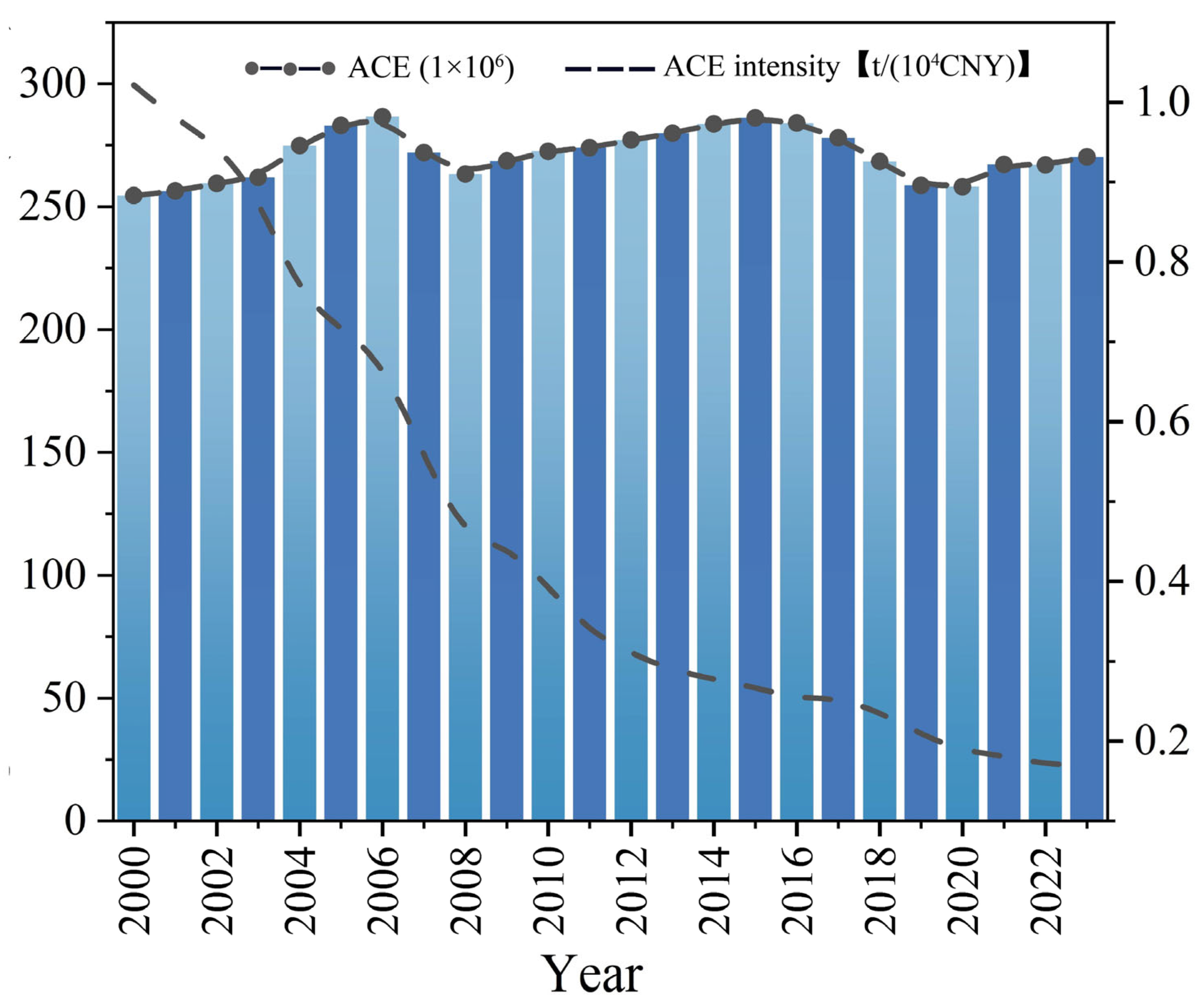
5.1. Characteristics of Temporal Changes

To elucidate the temporal evolution patterns of Chinese agricultural carbon emissions, this study analyzes the trends in total emissions and emission intensity from 2000 to 2023 (Figure 4). The results indicate that ACEs increased to 270.25 × 10⁶ tons in 2023, representing a 6.2% growth from 254.48 × 10⁶ tons in 2000, with an annual growth rate of 0.26% characterized by fluctuating upward trends. Three distinct phases emerged: Phase I (2000–2003) maintained relative stability with marginal increases; Phase II (2004–2008) exhibited an inverted V-shaped fluctuation; Phase III (2009–2023) showed decelerated growth, particularly after the 2015 national implementation of the Dual Reduction Policy that substantially decreased chemical fertilizer and pesticide usage, effectively curbing emission growth. Concurrently, carbon emission intensity demonstrated a sustained decline from 1.02 t (per 104 CNY output value) in 2000 to 0.17 t in 2023, achieving an 83.33% cumulative reduction.

5.2. Spatial Distribution Characteristics

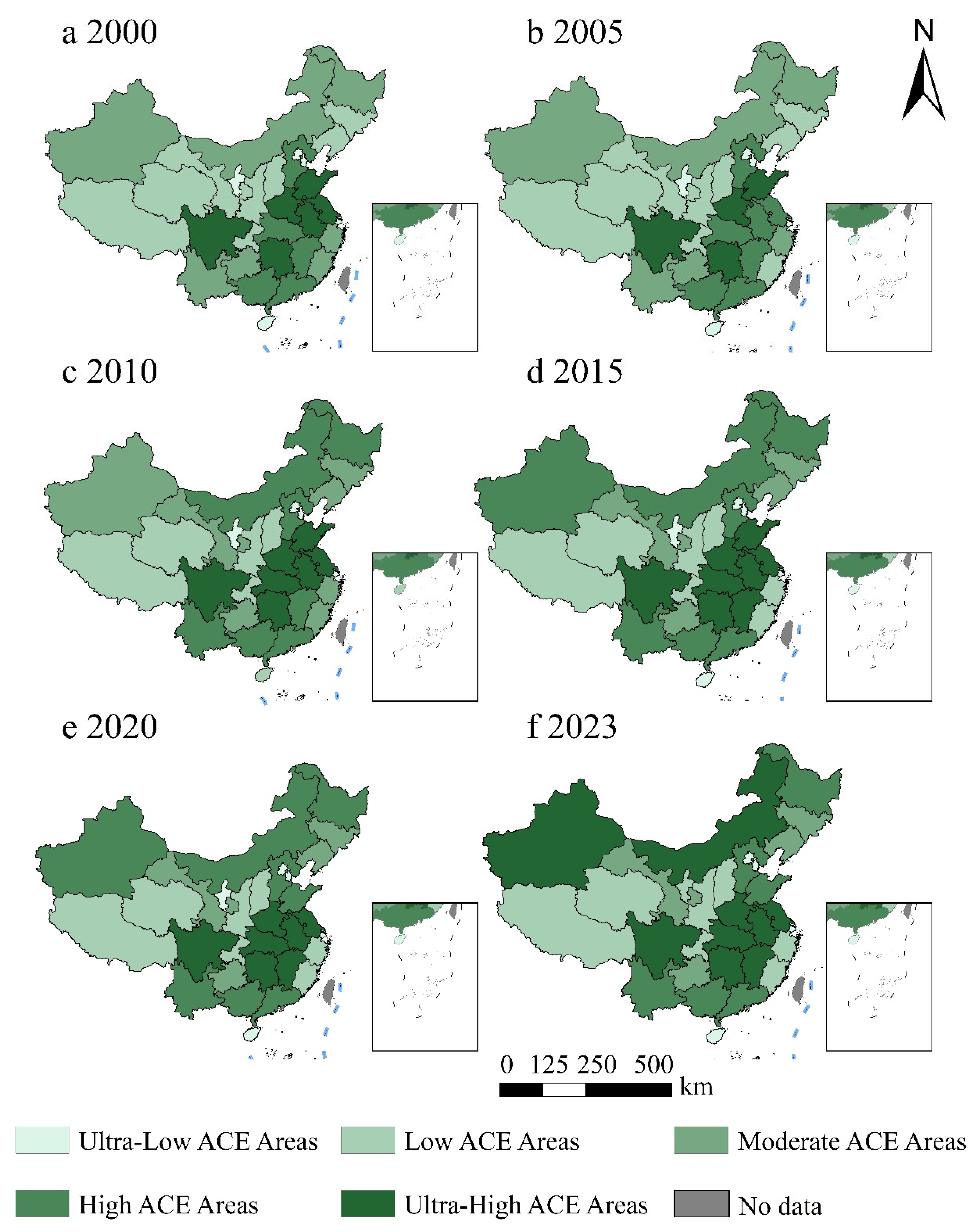
5.2.1. Spatial Variation Characteristics

The natural breaks classification method was applied to visualize province-level spatial distribution of ACEs (Figure 5), revealing significant spatial heterogeneity. Higher emission levels clustered in central regions, while northwestern regions exhibited relatively lower intensities. Inter-province differences in agricultural carbon emissions show an expanding trend, with certain provinces exhibiting a potential carbon lock-in effect. This effect arises from long-term reliance on high-carbon agricultural production models, leading some regions to become entrenched in high-emission path dependence, making a rapid transition to low-carbon agriculture challenging. For instance, Shandong Province, due to its prolonged dependence on fertilizer-intensive agriculture and traditional mechanized production, has developed significant carbon emission path dependence. In 2020, its agricultural carbon emission intensity was 0.35 t/10⁴ CNY, notably higher than the national average of 0.17 t/10⁴ CNY. This carbon lock-in effect stems from high-input agricultural infrastructure, farmers’ behavioral inertia, and lagging regional policies, which collectively hinder the adoption and application of low-carbon technologies. Hunan, Henan, and Sichuan Provinces emerged as the highest emitters, whereas Ningxia, Hainan, and Qinghai demonstrated relatively lower emission levels, indicating substantial interprovincial disparities. Seven of the top ten provinces ranked by carbon emission intensity in 2023 were concentrated within the eastern coastal economic belt. Temporal analysis (2000–2023) reveals an evolutionary trajectory of China’s ACEs characterized by “aggregate growth with westward expansion of high-emission clusters.” The spatial distribution of high-emission provinces transitioned from mononuclear agglomeration to multipolar diffusion, with identified provinces increasing from 6 in 2000 to 10 in 2023. Emerging clusters predominantly localized in the Yellow-Huaihai-Haihe Plain and Middle-Lower Yangtze Agricultural Zone.

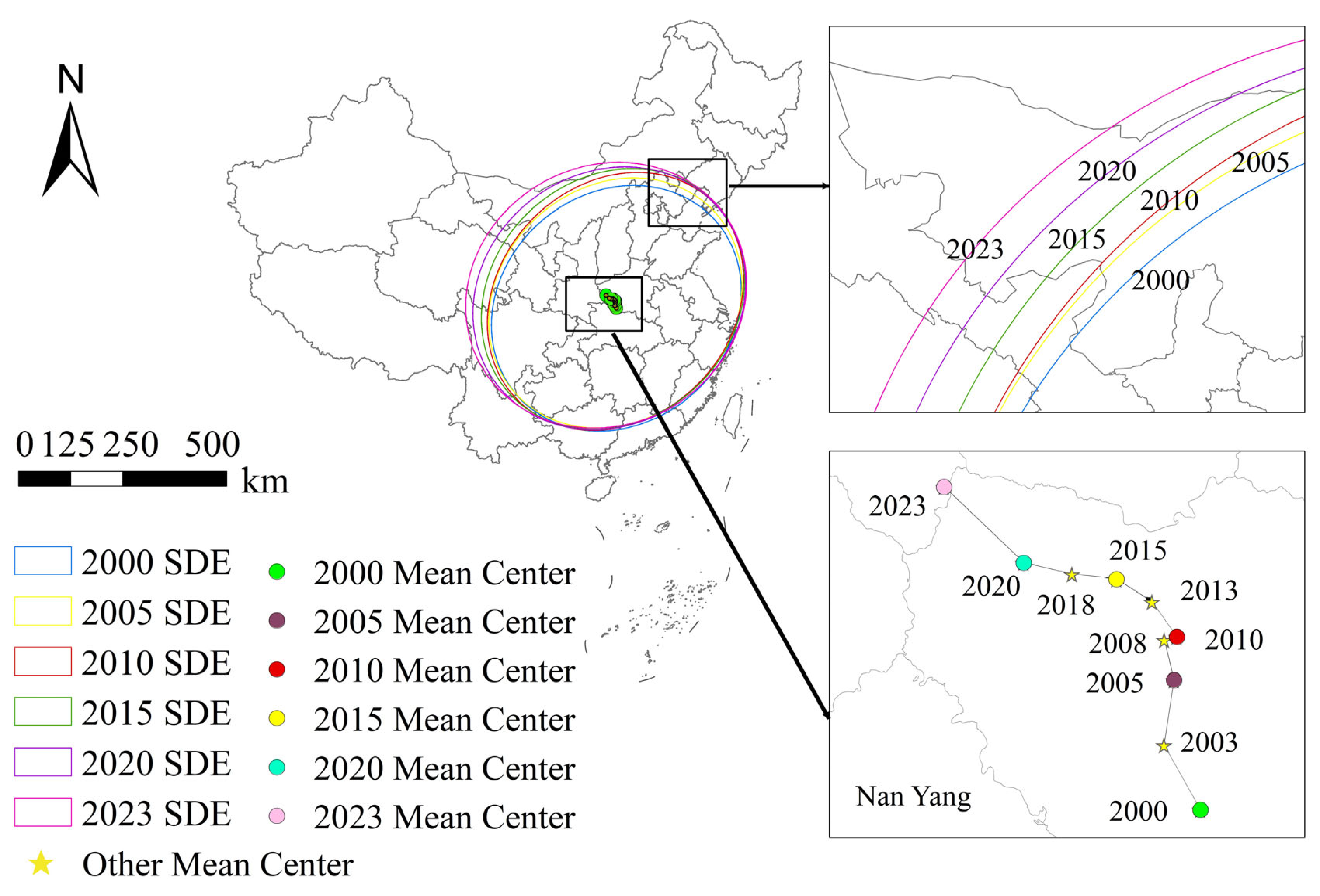
5.2.2. SDE and Center of Gravity Shift Analysis

Quantitative analysis employing SDE and gravity center migration was conducted to investigate spatial evolution patterns (Figure 6,

Table 6. Shape parameters of SDE for ACEs in China.

Year	Major Axis/km	Short Axis/km	Oblateness
2000	1111.909	966.306	0.131
2005	1133.391	977.855	0.137
2010	1169.980	982.920	0.160
2015	1180.032	1017.942	0.137
2020	1192.313	1055.615	0.115
2023	1208.217	1088.359	0.100

). The SDE demonstrated spatial concentration in central China, exhibiting predominant northeast-southwest orientation. Temporal analysis revealed sustained elongation of the major axis from 1111.909 km in 2000 to 1208.217 km in 2023, indicating intensified east-west spatial dispersion of emissions. Concurrently, the minor axis increased from 966.306 km to 1088.359 km over the same period, demonstrating analogous dispersive spatial dynamics. Ellipticity decreased from 0.131 to 0.100, with intermittent fluctuations, suggesting diminished spatial concentration of ACE.

The emission gravity center consistently remained localized within Nanyang City, Henan Province, while manifesting northwestward migration throughout the study period. This spatial configuration highlights the inherent stability and persistence of ACEs. The cumulative displacement distance of 138.66 km quantitatively reflects accelerated emission growth rates in western and northern regions compared to eastern and southern areas.

5.3. Spatially Correlated Features

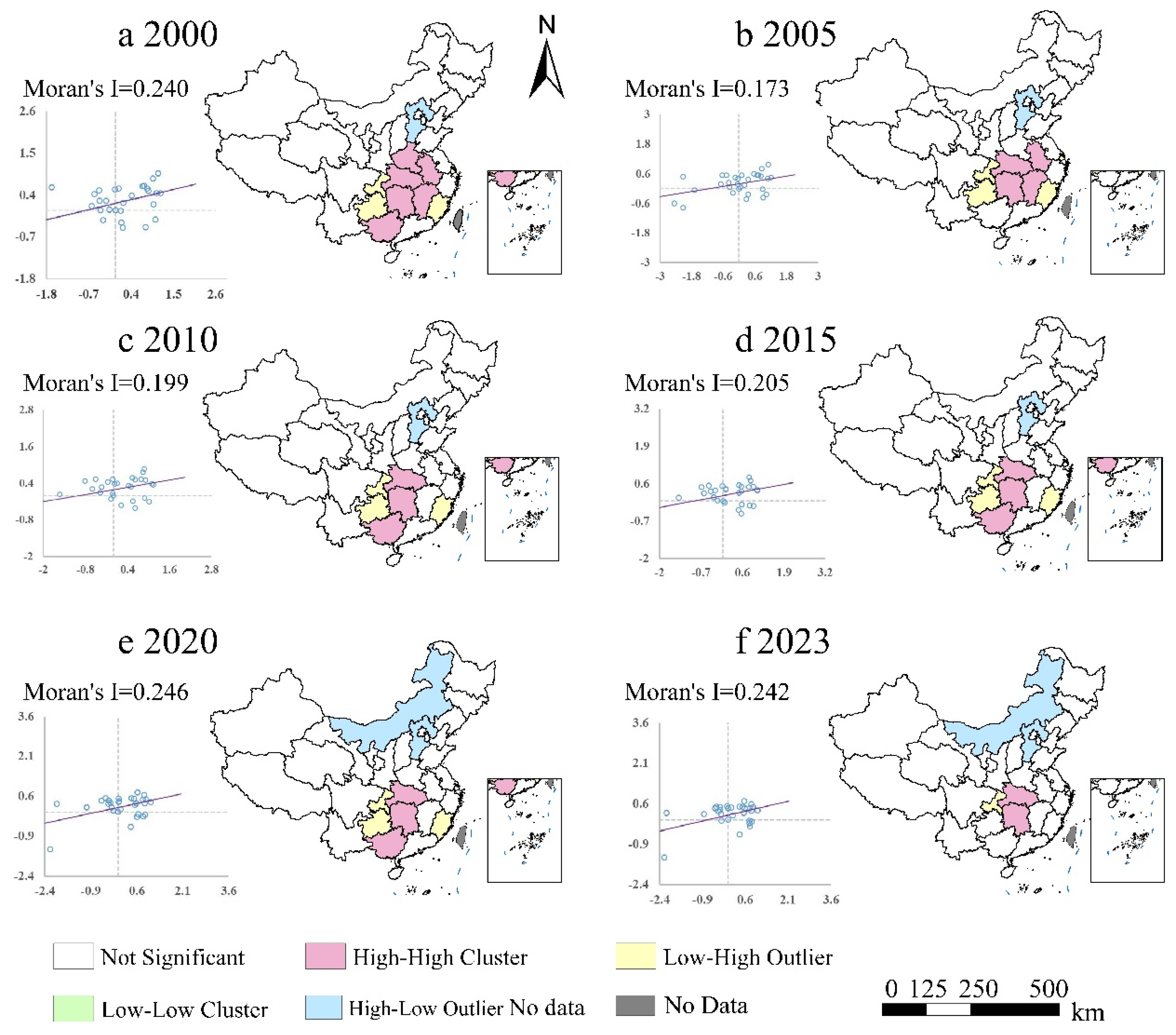
5.3.1. GSA Analysis

GSA analysis (Figure 7) revealed statistically significant spatial clustering patterns of ACE throughout the study period. The Moran’s I scatterplot illustrates spatial autocorrelation characteristics through four quadrants, with their meanings as follows. The first quadrant (High-High, HH) indicates high-emission provinces surrounded by other high-emission neighboring provinces, forming high-emission hotspot areas. The second quadrant (Low-High, LH) represents low-emission provinces adjacent to high-emission provinces, reflecting a spatial transition zone for emissions. The third quadrant (Low-Low, LL) signifies low-emission provinces surrounded by other low-emission neighboring provinces, forming low-emission cold spot areas. The fourth quadrant (High-Low, HL) denotes high-emission provinces neighboring low-emission provinces, highlighting spatial heterogeneity. The scatterplot visualization reveals that most provinces are distributed in the first quadrant (High-High clustering) and the second quadrant (Low-High clustering), confirming the presence of spatial clustering characteristics. Scatterplot visualization demonstrated predominant provincial distributions in the first quadrant (High-High clustering) and second quadrant (Low-High clustering), confirming the existence of spatial clustering characteristics. Collectively, the spatial positive correlation demonstrated an intensifying trend during 2000–2023, reaching peak significance in 2020. Despite maintenance of a positive spatial correlation, temporal variations in Moran’s I index values indicated persistent regional heterogeneity in emission levels.

5.3.2. LSA Analysis

LSA analysis of China’s provincial ACEs (2000–2023) elucidates spatiotemporal evolutionary characteristics of emission clustering patterns (Figure 7). Key findings are described below.

High-High clusters exhibited strong path dependency, persistently concentrated in central and eastern China throughout the study period. Notably, progressive transitions from High-High clusters to High-Low outliers occurred concurrently with dynamic redistribution of Low-High outliers, reflecting multifaceted heterogeneity in emission spatial configurations.

Specifically, an incipient spatial clustering configuration emerged in 2000, with high-value clusters demonstrating limited spatial extent and punctate distribution patterns. Concurrently, pronounced spatial heterogeneity manifested through outlier distributions containing either high-value enclaves surrounded by low-emission areas or conversely configured outliers. By 2005, high-value clusters exhibited marked spatial diffusion, with multiple provincial units transitioning from low-value or outlier status to clustered states. Low-Low clusters, while following analogous trends, exhibited comparably subdued expansion rates, whereas outliers maintained spatially dispersed distributions.

During 2010–2015, spatial clustering patterns of ACEs entered a phase of relative stabilization, with high-value clusters and low-value clusters exhibiting no substantial variation in spatial extent. Nevertheless, status transitions between cluster types occurred in specific provincial units, revealing ongoing dynamic restructuring processes within the spatial configuration. By 2023, high-value clusters demonstrated spatial consolidation and expansion, establishing multiple stable hotspot zones with intensified emission profiles. By comparison, low-value clusters displayed developmental inertia, failing to establish equilibrium configurations with their high-emission counterparts. Additionally, quantitative contraction of spatial outliers was observed, potentially indicating diminished spatial heterogeneity in emission distributions.

6. Analysis of the Results of the Impact Factors

6.1. Geodetector Analysis

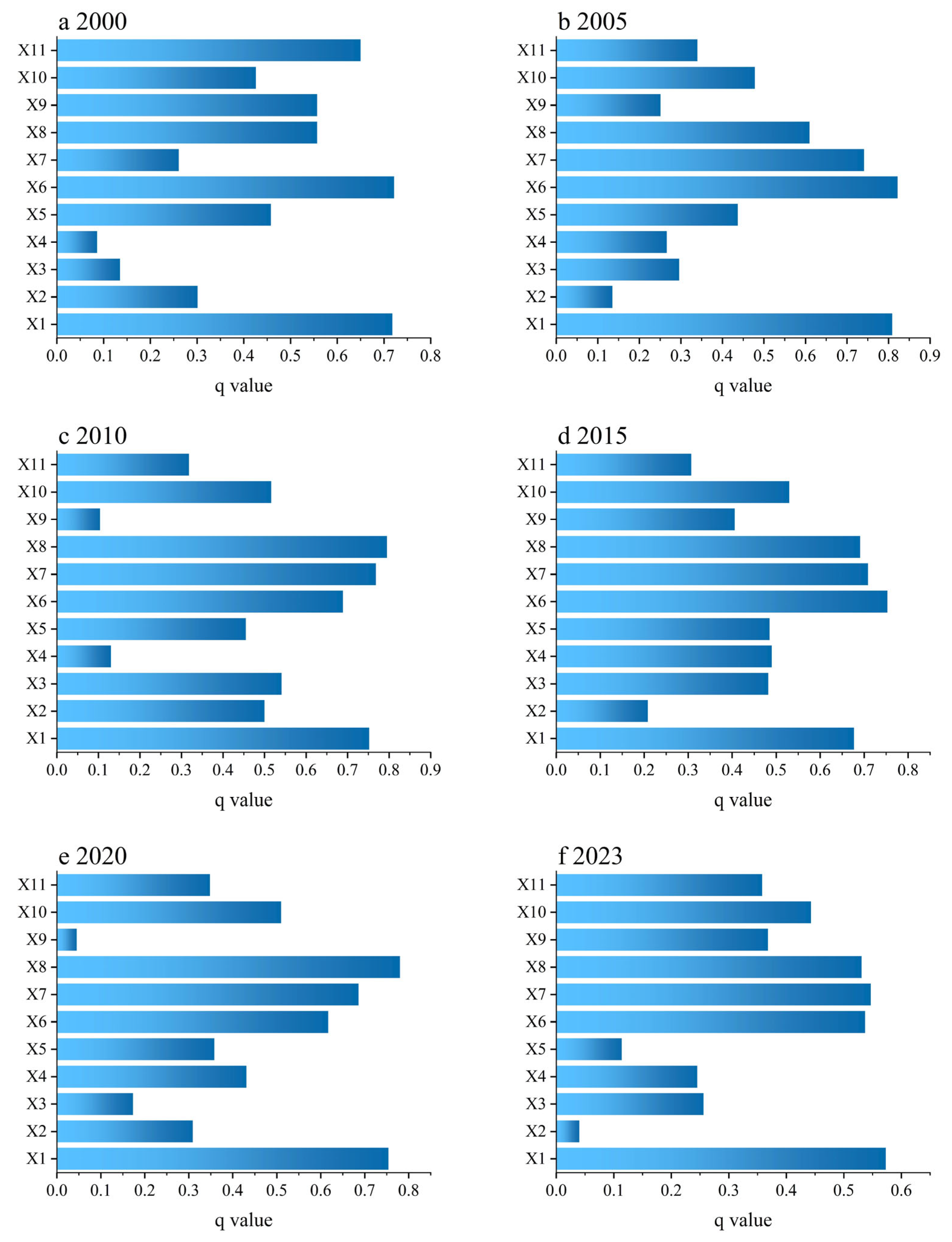
6.1.1. Single-Factor Identification

The empirical results reveal significant temporal heterogeneity in the impacts of 11 driving factors on ACEs (2000–2023), with all factors passing significance tests (p = 0.000) (Figure 8). Three distinct evolutionary phases were identified:

2000–2005: Economic scale dominance. COVAFAF (X1) maintained the highest explanatory power (q = 0.72–0.81), while PIE (X6) showed a declining marginal contribution, with q-values decreasing from 0.30 to 0.14. The high q-values of COVAFAF suggest that agricultural economic scale strongly drives spatial variations in emissions, guiding policymakers to prioritize economic restructuring for emission reduction.

2010–2020: Technology input dominance. TAMP (X8) and ACFA (X7) demonstrated enhanced explanatory capacity, peaking at q = 0.80/0.77 (2010) and q = 0.78/0.67 (2020), respectively, indicating accelerated agricultural modernization. During a 2015 transitional phase, joint dominance emerged between agricultural structure (X2, q = 0.21) and labor factors (X6, q = 0.75), revealing a critical policy window for industrial adjustment.

Terminal phase (2023): Economic scale factors regained prominence, with X1 and X6 rebounding to q = 0.57 and 0.54, respectively, highlighting cyclical evolutionary characteristics. This dynamic evolution elucidates interplay mechanisms between economic expansion, technological intensification, and policy intervention, providing temporal-stratified evidence for formulating stage-specific emission reduction strategies.

6.1.2. Factor Interaction Identification

While preceding analyses quantified individual factor influences, the spatial distribution of emissions is fundamentally shaped by complex interactions among multiple elements. Geodetector-based interaction analysis (Figure 9) reveals distinct phase evolution characteristics in the synergistic effects of emission drivers. The interaction between agricultural gross output value (COVAFA, X1) and economic development level (EDL, X3) dominated from 2000 to 2010, with q-values consistently above 0.92 (0.92 in 2000, 0.95 in 2005, 0.94 in 2010), reflecting a sustained synergistic effect of agricultural economic growth and regional development in shaping the spatial pattern of carbon emissions.

Three characteristic phases emerged: (1) 2000–2005, an economy-driven interactive phase with X1–X4/X6 synergies (q = 0.91) reflecting an extensive growth paradigm; (2) 2010–2015, a structural transition phase marked by enhanced X2 (AIS)–X6 interactions (q = 0.93) and emerging technological impacts, particularly the novel X4 (APE)–X8 (TAMP) synergy established in 2015; and (3) post-2020, a technology–climate interaction phase dominated by X8–X11 (Precip) synergies (q > 0.89, peaking at 0.95 in 2020 → 0.89 in 2023), indicating intensifying nonlinear coupling between modern agricultural technologies and climatic conditions. These high q-values in factor interactions highlight the amplified effect of combined drivers, suggesting that integrated policies targeting multiple factors can significantly enhance emission mitigation efforts.

Notably, the secondary strong X7 (ACFA)–X10 (Temp) interaction in 2010 (q = 0.93) suggests that climate change may indirectly regulate emission intensity through agricultural input efficiency modulation. This transition from economy-driven to technology–climate co-driven mechanisms provides critical interaction perspectives for formulating phase-specific emission reduction policies.

6.2. GTWR Analysis

Conventional GWR models capture spatial heterogeneity but do not account for temporal dynamics in ACEs. To address this limitation, we employ a GTWR model incorporating temporal weighting functions, which simultaneously addresses spatial heterogeneity and temporal non-stationarity, thus establishing an improved spatiotemporal analytical framework [57]. As evidenced by the model parameters in

Table 7. Model parameter results.

Model	AICc	R2	Adjusted R2
OLS	1156.0	0.4563	0.3334
GWR	1154.6	0.4546	0.3078
GTWR	23,098.5	0.9513	0.9509

, the GTWR model demonstrates superior goodness-of-fit, with an adjusted R² (>0.9) substantially exceeding those of the GWR and OLS counterparts.

Building on Geodetector-based factor analysis, we selected six key determinants with significant explanatory power as GTWR explanatory variables (as illustrated in Figure 10), enabling precise revelation of spatiotemporal differentiation patterns and the driving mechanisms underlying provincial ACEs in China.

COVAFA exhibits a significant positive correlation with ACE, displaying a spatially decreasing gradient from southeastern coastal regions toward central and western China. The positive GTWR coefficients for COVAFA indicate that higher agricultural economic output drives increased emissions, highlighting the necessity for low-carbon technologies in high-output regions. The Eastern Coastal Economic Belt demonstrates superior agricultural resource allocation and market concentration through enhanced industrialization and modernization [58], achieving both elevated COVAFA and correspondingly higher emission levels compared to western regions. This disparity originates from three primary mechanisms: (1) the southeastern coastal zone maintains integrated agricultural value chains, with advanced processing, logistics, and marketing infrastructure, establishing efficient industrialized operation frameworks [59]; (2) well-developed agricultural technology extension systems facilitate widespread adoption of precision farming and smart irrigation technologies, substantially enhancing production efficiency [60]; and (3) high-output production models inherently require intensive input utilization, generating economic growth while concomitantly increasing carbon emissions [61].

In contrast, northwest China exhibits distinct agricultural production characteristics. Traditional production paradigms constrain agricultural intensification and resource-use efficiency, leading to reduced COVAFA and comparatively lower emission intensities relative to southeastern coastal areas [62]. The region’s simplified agricultural structure, predominantly focused on conventional crop cultivation, further contributes to decreased emission intensity through reduced production complexity [63]. These regional disparities affirm the intrinsic linkage between agricultural economic development and carbon emissions, while underscoring significant heterogeneity in production modalities and emission profiles across geographical contexts.

RDI demonstrates significant negative correlations with ACEs, showing pronounced spatial heterogeneity across regions. The negative GTWR coefficients for RDI suggest that higher rural incomes facilitate investment in low-carbon practices, particularly in economically advanced regions, informing income-support policies for emission reduction. Southeastern coastal regions, characterized by advanced economic development and urbanization rates [64], possess structural advantages in urban–rural income parity and industrial diversification. Elevated income levels provide essential capital for adopting low-carbon agricultural technologies, while narrowed income disparities and optimized industrial structures collectively reduce emission intensity. Enhanced educational attainment in these regions [65] facilitates both technological adoption capacity and labor market adaptability, accelerating transitions toward sustainable agricultural practices.

In contrast, western provinces with delayed economic development remain dependent on agriculture as a primary income source [66], where constrained disposable income perpetuates reliance on carbon-intensive agricultural practices through limited technology adoption. Lower educational attainment further compounds these challenges through reduced non-agricultural employment competitiveness, reinforcing dependence on conventional farming systems. These disparities transcend pure economic dimensions, revealing fundamental gaps in socio-cultural development across regions. Regional educational disparities critically shape technological receptivity and labor market transitions [67], thereby exerting measurable impacts on agricultural emission patterns. These findings unravel the complex nexus between rural income dynamics and emission trajectories, while highlighting socio-cultural dimensions as crucial determinants in agricultural decarbonization processes.

PIE distribution exhibits a significant positive correlation with ACEs, demonstrating a spatially diminishing gradient radiating from Central China. The positive GTWR coefficients for PIE highlight that labor-intensive farming increases emissions, underscoring the need for mechanization and efficiency improvements in central regions. As China’s traditional agricultural core, central China maintains labor-intensive farming systems characterized by conventional practices reliant on human/animal power and inefficient mechanization, resulting in suboptimal energy utilization efficiency [68]. Excessive yet suboptimal utilization of agricultural inputs (fertilizers, pesticides) further elevates emission intensity per unit output [69]. Coupled with elevated population density, concentrated agricultural land parcels, and heightened land-use intensity, these drivers collectively sustain elevated aggregate emissions in the region [70].

In contrast, western China’s agricultural systems—constrained by geographical and developmental limitations—operate at smaller scales with extensive management practices under low population density conditions. Despite technological lag, decentralized landholdings and moderated land-use intensity result in substantially lower aggregate emissions compared to central China [71]. Notably, western regions demonstrate context-dependent negative emission effects, attributable to the synergistic effects of ecosystem carbon sequestration and low-intensity farming activities [72].

ACFA reflects distinct regional patterns in China’s agricultural production practices. The positive GTWR coefficients for ACFA indicate that fertilizer overuse significantly drives emissions, necessitating precise application techniques to reduce environmental impact. High-value clustering characterizes east China, north China, and northeast China, where plains dominate, with fertile soil resources including the black soils of northeast China and the cinnamon soils of the North China Plain, providing optimal conditions for large-scale intensive agricultural production. However, prolonged intensive farming has caused persistent soil organic matter depletion, compelling farmers to over-rely on chemical fertilizers to maintain high yields, a practice that substantially amplifies ACEs [73]. Provinces with heightened agricultural intensification (e.g., Anhui, Hebei, Shandong) exhibit fertilizer application rates significantly exceeding national averages, emerging as critical sources of ACEs.

In contrast, distinct patterns manifest in western China and traditional agricultural zones of southern China. These regions feature predominantly mountainous and hilly terrain with nutrient-poor soils (e.g., red soils, yellow soils), coupled with widespread soil erosion, collectively resulting in low fertilizer utilization efficiency. Constrained by these natural limitations, farmers adopt reduced fertilizer inputs and extensive farming practices, thereby diminishing the emission-enhancing effects of fertilizer application compared to intensive agricultural regions [74].

The spatial distribution of TAMP demonstrates an elevational gradient, with western regions exhibiting higher values compared to their northern counterparts. The positive GTWR coefficients for TAMP in underdeveloped regions suggest that mechanization increases emissions, highlighting the need for clean energy integration in machinery operations. Mechanization in agriculturally underdeveloped regions generally amplifies carbon emission intensity, whereas intermediate-to-high development zones show no statistically significant effects. Sichuan and Qinghai exhibit exceptional mechanization-induced emission amplification through dual mechanisms: (1) geomorphological constraints (Sichuan’s mountainous terrain; Qinghai’s high-altitude cryogenic environment) necessitate energy-intensive machinery operations [75], and (2) the predominance of carbon-intensive energy matrices in regional power systems exacerbates mechanization’s carbon footprint.

In contrast, northern regions (particularly Inner Mongolia) demonstrate mechanization-mediated emission mitigation. This phenomenon arises from tripartite determinants: topographic homogeneity enabling scaled mechanization [76]; clean energy integration displacing fossil fuels; and systematic crop residue management minimizing open-field burning [77].

Thermal conditions follow latitudinal zonality, with a progressive northward Temp decline. The GTWR coefficients for Temp indicate that warmer climates increase emissions through extended growing seasons and input demands, guiding climate-adaptive agricultural policies. Southern regions benefit from extended growing seasons under warm-humid regimes, facilitating high-yield crop cultivation. Elevated temperatures enhance photosynthetic efficiency and phenological duration, synergistically increasing both agricultural productivity and associated emissions [78]. Northern territories constrained by truncated growing seasons and thermal limitations exhibit reduced cropping intensity and correspondingly lower emissions [79]. This spatial pattern unequivocally demonstrates climate-driven modulation of agricultural regimes and their carbon consequences.

Xinjiang manifests exceptional Temp sensitivity in agricultural emission dynamics. A tripartite mechanism underpins this phenomenon: (1) persistent reliance on input-intensive practices (fertilizers, irrigation, machinery); (2) thermal acceleration of carbon-intensive agrochemical cycles; and (3) aridity-driven irrigation that demands amplifying temperature–emission synergies [80].

7. Discussion

Agricultural production systems exhibit a dual role as carbon sources and sinks, with substantial uncertainties inherent in source quantification. Current scholarship predominantly quantifies emissions through five operational dimensions: agricultural inputs, rice cultivation, straw burning, enteric fermentation, and manure management [45,49,81]. Given the lack of standardized methodologies for straw burning and soil carbon emission quantification, coupled with divergent emission coefficients across institutions, this study prioritizes analysis of three principal source categories.

7.1. Spatiotemporal Evolution of ACEs in China

(1)

From a temporal perspective, China’s ACEs exhibit an overall trend of fluctuating growth, while carbon emission intensity has gradually declined, consistent with findings from Peng et al. [82]. The emission flux variability reflects synergistic policy–technology interactions, particularly post-2015 fertilizer/pesticide reduction initiatives. In contrast to previous studies, this research identifies a more substantial decline in emission intensity (83.33%), with the apparent paradox of decreasing intensity alongside increasing total emissions attributable to (1) the expansion of agricultural output value (COVAFAF growing at an average annual rate of 6.5%), which drives increased inputs and elevates total emissions; and (2) technological advancements such as precision fertilization and energy-efficient machinery, which reduce emissions per unit of output, significantly lowering intensity. This is closely linked to the effectiveness of policy regulation, indicating that technological improvements and policy support have a significant combined impact on reducing carbon emissions.

(2)

Significant variations in agricultural carbon emissions are observed across provinces, aligning closely with the spatial differentiation characteristics identified by Liu et al. [81,83]. Concurrently, the spatial pattern of agricultural carbon emissions exhibits high-value clustering in the southeastern region, consistent with the findings of Wen et al. [84]. The gradual eastward and westward expansion of agricultural carbon emissions reflects differences in agricultural production modes across regions. The spatial clustering effect of agricultural carbon emissions has weakened over time, corroborating Xia’s conclusions [85]; however, this study covers a longer historical period, suggesting that the spatial distribution of agricultural carbon emissions is influenced by multiple factors over an extended timescale, potentially leading to gradual weakening of the spatial clustering effect. Compared to India [86], where high emissions are concentrated in irrigation-intensive areas, China’s eastern high-emission zones are centered in economically developed regions. This highlights the need for developing countries to optimize emission reduction strategies tailored to regional characteristics.

7.2. Determinants of ACEs in Chinese Provinces

(1)

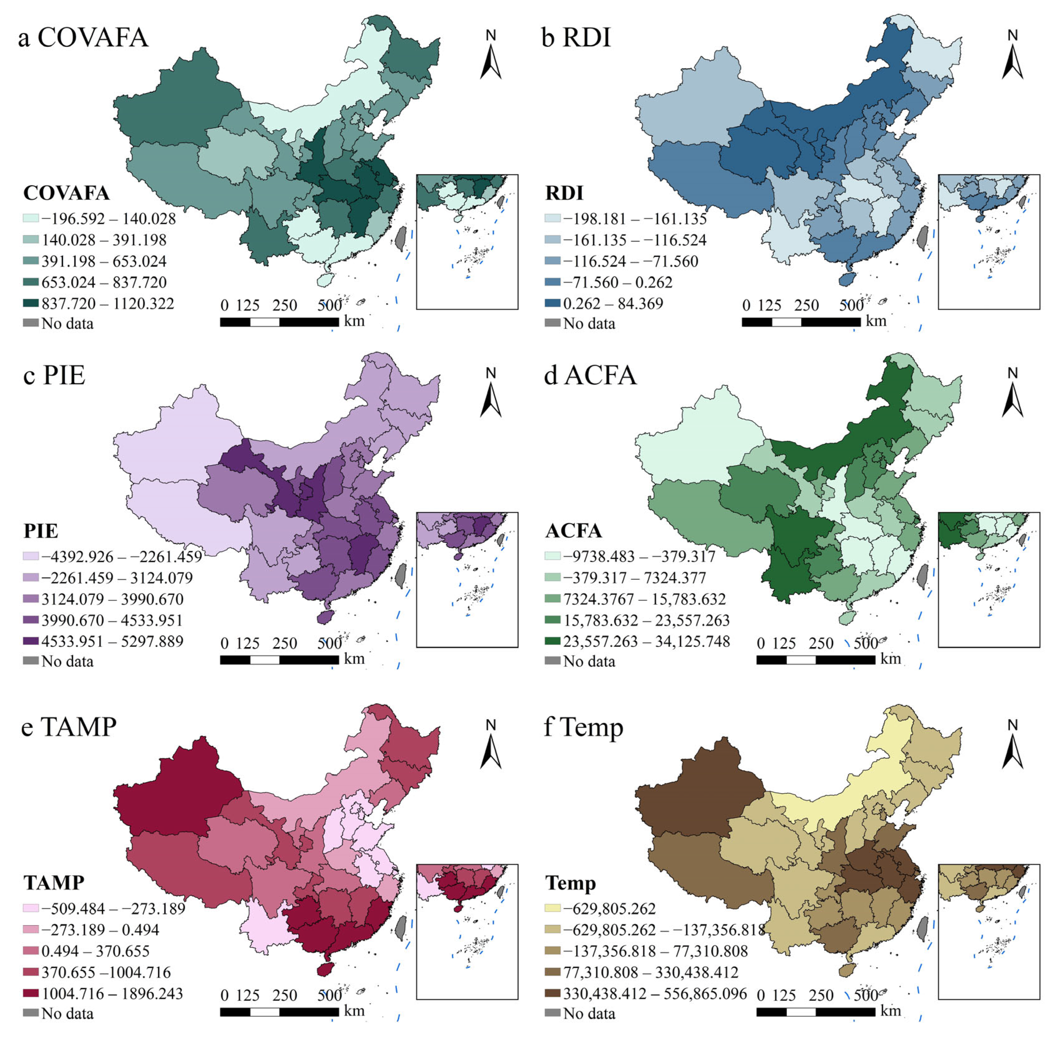
Economic factors are the primary drivers of increased agricultural carbon emissions, with the COVAFAF exerting the greatest influence on agricultural carbon emissions. Moreover, as economic scale expands and agricultural modernization progresses, this influence exhibits periodic fluctuations, consistent with the findings of Li et al. regarding the driving role of economic scale in carbon emissions [87,88]. Furthermore, spatiotemporal differentiation in rural disposable income underscores policy coordination complexity. Coastal eastern regions demonstrate negative income–emission correlations, reflecting green consumption awareness enhancement in emission reduction. Conversely, western regions exhibit positive correlations, indicating persistent dependence on carbon-intensive agricultural production modes. This paradox reveals regional disparities in achieving income-growth–emission-reduction synergy, necessitating decoupling through non-agricultural industry support and green subsidy policies.

(2)

Agricultural input factors are key determinants of agricultural carbon emissions. The positive influence of total agricultural machinery power, employment in the primary sector, and fertilizer application on agricultural carbon emissions aligns with the findings of Guo et al. High-tech machinery in the eastern regions reduces emissions [89,90], while traditional machinery in the western regions exacerbates emissions, going beyond the single-input analysis of Tang et al. [91] and providing a reference for machinery optimization in Brazil. For instance, agricultural mechanization proliferation typically coincides with intensified fertilizer, pesticide, and plastic film applications. While collectively enhancing productivity, these practices elevate emission levels [92]. Concurrently, primary sector employment growth often drives land reclamation expansion and resource utilization intensification, subsequently amplifying demands for machinery, chemicals, and irrigation—thereby escalating emission scales. Effective agricultural decarbonization thus requires comprehensive consideration of input factor synergies.

(3)

Climatic variables, particularly Temp and Precip, significantly shape emission spatial distributions. Although Gołasa et al. [3] rarely directly address the role of climatic factors, both the existing literature and this study indicate that the impact of climate change on agricultural carbon emissions is increasingly significant. Temp elevation may prolong growing seasons and enhance photosynthesis, boosting agricultural yields, yet simultaneously drives increased agrochemical inputs that elevate emissions. Precip patterns directly determine irrigation requirements and production methods, with water-stressed regions exhibiting energy-intensive irrigation dependencies. Furthermore, Precip variability and extreme weather events intensify spatiotemporal emission heterogeneity [56]. Compared to the single climate variable analysis by Panchasara et al. [15], this study quantifies interactive effects, providing climate adaptation strategies for rice cultivation areas in Vietnam.

7.3. Spatiotemporal Heterogeneity of Influencing Factors

Previous studies employing traditional econometric regression models and spatial econometric models have effectively identified key drivers of ACEs. However, these models are limited in capturing the spatiotemporal heterogeneity of driving factors, thus failing to elucidate the dynamic evolution of dominant factors across different periods and their differential impacts on ACE [93]. In contrast, the Geodetector and GTWR models to effectively reveal the spatiotemporal heterogeneity of ACE, thereby providing a more robust scientific basis for formulating regionally tailored carbon reduction policies.

The Geodetector quantifies the explanatory power of factors on spatial differentiation, analyzes synergistic effects among different factors, and reveals temporal variations in driving factors’ explanatory capacities [94]. For instance, this study demonstrates that gross agricultural output value constituted the core driver of agricultural carbon emissions during 2000–2005, while technological inputs gradually emerged as dominant factors during 2010–2020. This revelation of phased transitions provides policymakers with crucial temporal-dimensional evidence. The GTWR model further captures the spatiotemporal heterogeneity of driving factors through geographically and temporally weighted regression [95]. While conventional regression analysis might indicate significant positive impacts of gross agricultural output value on carbon emissions, it fails to identify intensity variations between southeastern coastal regions and western inland areas. The GTWR model reveals such spatial disparities, demonstrating that rural residents’ disposable income exhibits significant emission-reduction effects in eastern coastal regions but incremental effects in western regions.

By integrating the Geodetector and GTWR models, this study overcomes the limitations of traditional regression and spatial econometric approaches, not only uncovering the complex spatiotemporal heterogeneity of ACE, but also providing a comprehensive analysis of the spatial distribution and evolutionary patterns of driving factors [96]. This integrated approach establishes a robust scientific foundation for the precise formulation of regional agricultural emission-reduction policies, with broad application potential. The empirical results suggest that eastern coastal regions should prioritize green agricultural technologies to reduce high-carbon production modes, while western regions require enhanced rural income levels and agricultural modernization to mitigate emissions from traditional farming practices. These regionally differentiated policy recommendations highlight the crucial role of combining Geodetector and GTWR models in agricultural low-carbon transition and regional green development, offering novel perspectives and methodological support for subsequent research. Compared to the static analysis of Miao et al. [97], this study dynamically captures policy windows, providing a phased emission reduction framework for developing countries.

7.4. Research Limitations and Future Directions

7.4.1. Research Limitations

First, this study’s calculations exclude straw burning and soil carbon emissions, which may contribute 15–20% to emissions in southern rice cultivation areas. This limitation could lead to an underestimation of high-emission characteristics in the eastern coastal regions, weakening the specificity of policy recommendations, such as potentially underestimating the need for promoting precision agriculture technologies. Future studies can integrate remote sensing with on-site monitoring to correct accounting biases, which is expected to improve emission estimation accuracy by approximately 10–15%. Incorporating remote sensing inversion and field monitoring data in future research can enhance accounting for straw burning and soil carbon fluxes. Second, the discretization of factors in Geodetector may obscure the details of continuous variables, resulting in an explanatory power bias of about 5%. Additionally, GTWR responds slowly to abrupt policy changes (e.g., a 20% drop in fertilizer use due to the 2020 pandemic), with coefficient biases of around 15%. This study captures spatiotemporal heterogeneity but does not conduct sensitivity analysis to validate result robustness, necessitating the integration of real-time data for model calibration in the future. Furthermore, while Xia et al. [85] suggest a contraction of high-emission areas, this study finds a westward expansion of hotspots, a discrepancy possibly due to differences in time spans or variable selection. Future studies should incorporate policy intensity variables for validation. Nevertheless, by leveraging long-term data and multi-method integration, this study still provides a reliable basis for regional low-carbon policies.

7.4.2. Future Research Directions

Due to data and scope constraints, this study does not deeply analyze policy intensity, other climatic variables, or socioeconomic factors, yet these areas hold significant potential for exploration. First, standardizing provincial policy data is challenging, and this study could not quantify the frequency of emission regulations or subsidy levels. However, Jiangsu’s experience shows that high-frequency policies can reduce emissions by 10%, suggesting that future research could explore the interaction between policies and agricultural output value, offering insights for policy design in countries like India. Second, climatic variables such as drought frequency were not included due to the complexity of processing CMIP6 data. However, India’s case of reducing methane emissions by 10% through drought management highlights their importance, suggesting future assessments of the impacts of drought and heavy rainfall, applicable to countries like Vietnam. Third, technology adoption rates and education levels were not analyzed due to data limitations, but Zhejiang’s experience—where high education levels reduced emissions by 15%—underscores their value. Future studies should introduce weight matrices to test model stability, supporting low-carbon agricultural practices in countries like Brazil. These directions will enhance the global applicability of the research, providing a more comprehensive guidance framework for developing countries to address agricultural intensification and climate challenges.

8. Conclusions and Policy Recommendations

8.1. Conclusions

Under the “dual carbon” strategy framework, ACEs, as a significant source of greenhouse gases, require systematic identification and precise analysis of their spatiotemporal evolution and underlying driving mechanisms. Utilizing provincial panel data from 2000–2023 in China, this study comprehensively investigates China’s ACE through three dimensions—temporal evolution, spatial distribution, and driving mechanisms—by integrating carbon emission accounting models, spatial statistical analysis methods, and spatiotemporal heterogeneity modeling techniques. The main findings are as follows:

(1)

Temporally, China’s total ACEs exhibited “fluctuating growth”, with an average annual rate of 0.26%, while emission intensity demonstrated a remarkable cumulative reduction of 83.33%. This indicates significant declines in carbon emissions per unit output alongside maintained production growth, reflecting synergistic effects of policy interventions and technological advancements.

(2)

Spatially, ACEs exhibited a pronounced “higher in the southeast, lower in the northwest” imbalance, with a dynamic evolution characterized by expanding high-emission zones and a westward shift of hotspots. SDE and centroid migration analyses revealed a “northeast-southwest” belt-shaped distribution, with the emission centroid consistently located in Nanyang, Henan Province, while gradually shifting northwestward, suggesting an emerging emission growth potential in western regions. Spatial autocorrelation results confirmed strengthening agglomeration patterns, particularly in the traditional agricultural regions of central-eastern China.

(3)

The driving mechanisms of ACEs exhibited pronounced spatiotemporal heterogeneity. The Geodetector results identified gross agricultural output value as the primary single-factor driver, displaying cyclical fluctuations characterized by phases of economic dominance, technological advancement, and structural adjustment. Factor interaction analysis revealed synergistic effects between agricultural economic scale and key factors such as regional economic development, industrial structure, and climatic conditions. GTWR modeling further disclosed that rural disposable income contributed to emission reductions in eastern regions, whereas variables such as gross agricultural output value, primary industry employment, fertilizer application, and total agricultural machinery power primarily drove emission increases across most regions, with notable variations in direction and intensity across spatiotemporal contexts.

8.2. Policy Recommendations

(1)

Promoting precision fertilization to mitigate high carbon emission risks from excessive fertilizer use

The results indicate that the application of chemical fertilizers (ACFA) exerts a significant positive impact on agricultural carbon emissions, particularly in highly intensive agricultural provinces such as Shandong, Anhui, and Hebei. Therefore, it is imperative for the eastern coastal regions—especially these provinces—to accelerate the dissemination and application of precision fertilization technologies. This can be achieved by establishing regional soil nutrient databases and promoting soil testing and formulated fertilization techniques to ensure the precise and efficient use of fertilizers [98]. In parallel, financial support mechanisms, such as subsidies or dedicated funding programs, should be introduced to reduce the initial costs incurred by farmers adopting such technologies. However, challenges such as technical dissemination barriers and farmers’ limited acceptance may hinder widespread adoption. Thus, strengthening grassroots agricultural extension systems and conducting regular farmer training and demonstration activities are essential to enhance awareness and willingness to adopt precision technologies [99].

(2)

Advancing the clean transition of agricultural machinery to reduce emissions from traditional operations

This study finds that total agricultural machinery power (TAMP) contributes significantly to agricultural carbon emissions in southwestern provinces such as Sichuan and Qinghai, while northern regions exhibit some emission reduction effects due to the adoption of clean energy sources. It is recommended that the southwestern regions actively promote the clean transformation of agricultural machinery. For instance, electric-powered equipment should replace conventional diesel-powered machinery, and solar resources can be harnessed through photovoltaic agriculture integrated systems to facilitate the transition from high-carbon to low-carbon agricultural practices [100]. To address the challenge of high initial investment in equipment replacement, policies such as machinery upgrade subsidies and low- or zero-interest loans should be explored. Additionally, establishing regional platforms for machinery sharing can reduce individual farmers’ equipment costs, while demonstration sites may enhance farmer acceptance of clean-energy agricultural equipment [101].

(3)

Optimizing industrial structure to decouple economic growth from agricultural carbon emissions

In this study, the gross output value of agriculture, forestry, animal husbandry, and fishing (COVAFA) is identified as a primary driver of agricultural carbon emissions. Eastern economically developed regions exhibit both higher agricultural output and greater carbon intensity compared to western areas. Therefore, these eastern coastal regions should optimize their industrial structures to decouple economic growth from carbon emissions. On one hand, the development of circular agriculture and high-efficiency-facility agriculture should be promoted to enhance the added value of agricultural output [102]; on the other hand, agricultural service industries and deep processing of agricultural products should be encouraged to reduce the proportion of direct emissions from primary production. Recognizing the potential challenges posed by industrial restructuring—such as disruptions in agricultural supply chains, market volatility, and farmers’ adaptation difficulties—governments should provide comprehensive support through policies, funding, and market infrastructure. This includes establishing special transformation funds, creating production–marketing linkage platforms, and implementing green certification systems for agricultural products to ensure the stability and sustainability of the structural transition process [103].

References

1. Bhatti, U.A.; Bhatti, M.A.; Tang, H.; Syam, M.S.; Awwad, E.M.; Sharaf, M.; Ghadi, Y.Y. Global Production Patterns: Understanding the Relationship between Greenhouse Gas Emissions, Agriculture Greening and Climate Variability. Environ. Res. 2024, 245, 118049. [Google Scholar] [CrossRef] [PubMed]
2. Wang, J.; Xu, Y. Internet Usage, Human Capital and CO2 Emissions: A Global Perspective. Sustainability 2021, 13, 8268. [Google Scholar] [CrossRef]
3. Gołasa, P.; Wysokiński, M.; Bieńkowska-Gołasa, W.; Gradziuk, P.; Golonko, M.; Gradziuk, B.; Siedlecka, A.; Gromada, A. Sources of Greenhouse Gas Emissions in Agriculture, with Particular Emphasis on Emissions from Energy Used. Energies 2021, 14, 3784. [Google Scholar] [CrossRef]
4. Wang, Y.; Guo, C.; Chen, X.; Jia, L.; Guo, X.; Chen, R.; Zhang, M.; Chen, Z.; Wang, H. Carbon Peak and Carbon Neutrality in China: Goals, Implementation Path and Prospects. China Geol. 2021, 4, 720–746. [Google Scholar] [CrossRef]
5. Laborde, D.; Mamun, A.; Martin, W.; Piñeiro, V.; Vos, R. Agricultural Subsidies and Global Greenhouse Gas Emissions. Nat. Commun. 2021, 12, 2601. [Google Scholar] [CrossRef] [PubMed]
6. Wijerathna-Yapa, A.; Pathirana, R. Sustainable Agro-Food Systems for Addressing Climate Change and Food Security. Agriculture 2022, 12, 1554. [Google Scholar] [CrossRef]
7. West, T.O.; Marland, G. A Synthesis of Carbon Sequestration, Carbon Emissions, and Net Carbon Flux in Agriculture: Comparing Tillage Practices in the United States. Agric. Ecosyst. Environ. 2002, 91, 217–232. [Google Scholar] [CrossRef]
8. Zhao, R.-Q.; Qin, M.-Z. Temporospatial Variation of Partial Carbon Source/Sink of Farmland Ecosystem in Coastal China. J. Ecol. Rural. Environ. 2007, 23, 1–6. [Google Scholar]
9. Cui, Y.; Khan, S.U.; Deng, Y.; Zhao, M.; Hou, M. Environmental Improvement Value of Agricultural Carbon Reduction and Its Spatiotemporal Dynamic Evolution: Evidence from China. Sci. Total Environ. 2021, 754, 142170. [Google Scholar] [CrossRef]
10. Li, H.; Jin, X.; Zhao, R.; Han, B.; Zhou, Y.; Tittonell, P. Assessing Uncertainties and Discrepancies in Agricultural Greenhouse Gas Emissions Estimation in China: A Comprehensive Review. Environ. Impact Assess. Rev. 2024, 106, 107498. [Google Scholar] [CrossRef]
11. Ning, J.; Zhang, C.; Hu, M.; Sun, T. Accounting for Greenhouse Gas Emissions in the Agricultural System of China Based on the Life Cycle Assessment Method. Sustainability 2024, 16, 2594. [Google Scholar] [CrossRef]
12. Zhang, C.; Zhao, L.; Zhang, H.; Chen, M.; Fang, R.; Yao, Y.; Zhang, Q.; Wang, Q. Spatial-Temporal Characteristics of Carbon Emissions from Land Use Change in Yellow River Delta Region, China. Ecol. Indic. 2022, 136, 108623. [Google Scholar] [CrossRef]
13. Tian, Y.; Zhang, J.; He, Y. Research on Spatial-Temporal Characteristics and Driving Factor of Agricultural Carbon Emissions in China. J. Integr. Agric. 2014, 13, 1393–1403. [Google Scholar] [CrossRef]
14. Luo, Y.; Long, X.; Wu, C.; Zhang, J. Decoupling CO2 Emissions from Economic Growth in Agricultural Sector across 30 Chinese Provinces from 1997 to 2014. J. Clean. Prod. 2017, 159, 220–228. [Google Scholar] [CrossRef]
15. Panchasara, H.; Samrat, N.H.; Islam, N. Greenhouse Gas Emissions Trends and Mitigation Measures in Australian Agriculture Sector—A Review. Agriculture 2021, 11, 85. [Google Scholar] [CrossRef]
16. Lin, B.; Xu, B. Factors Affecting CO2 Emissions in China’s Agriculture Sector: A Quantile Regression. Renew. Sustain. Energy Rev. 2018, 94, 15–27. [Google Scholar] [CrossRef]
17. Xiong, C.; Yang, D.; Xia, F.; Huo, J. Changes in Agricultural Carbon Emissions and Factors That Influence Agricultural Carbon Emissions Based on Different Stages in Xinjiang, China. Sci. Rep. 2016, 6, 36912. [Google Scholar] [CrossRef]
18. Shan, T.; Xia, Y.; Hu, C.; Zhang, S.; Zhang, J.; Xiao, Y.; Dan, F. Analysis of Regional Agricultural Carbon Emission Efficiency and Influencing Factors: Case Study of Hubei Province in China. PLoS ONE 2022, 17, e0266172. [Google Scholar] [CrossRef]
19. Han, G.; Xu, J.; Zhang, X.; Pan, X. Efficiency and Driving Factors of Agricultural Carbon Emissions: A Study in Chinese State Farms. Agriculture 2024, 14, 1454. [Google Scholar] [CrossRef]
20. Yizhang, P.; Ping, L. Study on the Relationship between Agricultural Mechanization, Fiscal Expenditure and Agricultural Carbon Emission: Empirical Analysis Based on VAR Model. J. Chin. Agric. Mech. 2025, 46, 313. [Google Scholar] [CrossRef]
21. Guan, N.; Liu, L.; Dong, K.; Xie, M.; Du, Y. Agricultural Mechanization, Large-Scale Operation and Agricultural Carbon Emissions. Cogent Food Agric. 2023, 9, 2238430. [Google Scholar] [CrossRef]
22. Lesschen, J.P.; van den Berg, M.; Westhoek, H.J.; Witzke, H.P.; Oenema, O. Greenhouse Gas Emission Profiles of European Livestock Sectors. Anim. Feed. Sci. Technol. 2011, 166–167, 16–28. [Google Scholar] [CrossRef]
23. Xiong, C.; Yang, D.; Huo, J. Spatial-Temporal Characteristics and LMDI-Based Impact Factor Decomposition of Agricultural Carbon Emissions in Hotan Prefecture, China. Sustainability 2016, 8, 262. [Google Scholar] [CrossRef]
24. Raihan, A.; Muhtasim, D.A.; Farhana, S.; Hasan, M.A.U.; Pavel, M.I.; Faruk, O.; Rahman, M.; Mahmood, A. An Econometric Analysis of Greenhouse Gas Emissions from Different Agricultural Factors in Bangladesh. Energy Nexus 2023, 9, 100179. [Google Scholar] [CrossRef]
25. Yang, X.; Jia, Z.; Yang, Z.; Yuan, X. The Effects of Technological Factors on Carbon Emissions from Various Sectors in China—A Spatial Perspective. J. Clean. Prod. 2021, 301, 126949. [Google Scholar] [CrossRef]
26. Kheyruri, Y.; Sharafati, A.; Neshat, A.; Hameed, A.S.; Rahman, A. Analyzing the Impact of Socio-Environmental Parameters on Wheat and Barley Cultivation Areas Using the Geographical Detector Model. Phys. Chem. Earth Parts A/B/C 2024, 135, 103630. [Google Scholar] [CrossRef]
27. Feng, L.; Wang, Y.; Zhang, Z.; Du, Q. Geographically and Temporally Weighted Neural Network for Winter Wheat Yield Prediction. Remote Sens. Environ. 2021, 262, 112514. [Google Scholar] [CrossRef]
28. Yin, Z.; Ding, J.; Liu, Y.; Wang, R.; Wang, Y.; Chen, Y.; Qi, J.; Wu, S.; Du, Z. GNNWR: An Open-Source Package of Spatiotemporal Intelligent Regression Methods for Modeling Spatial and Temporal Nonstationarity. Geosci. Model Dev. 2024, 17, 8455–8468. [Google Scholar] [CrossRef]
29. Liu, J.; Wang, J.; Zhai, T.; Li, Z.; Huang, L.; Yuan, S. Gradient Characteristics of China’s Land Use Patterns and Identification of the East-West Natural-Socio-Economic Transitional Zone for National Spatial Planning. Land Use Policy 2021, 109, 105671. [Google Scholar] [CrossRef]
30. Guo, A.; Yue, W.; Yang, J.; Xue, B.; Xiao, W.; Li, M.; He, T.; Zhang, M.; Jin, X.; Zhou, Q. Cropland Abandonment in China: Patterns, Drivers, and Implications for Food Security. J. Clean. Prod. 2023, 418, 138154. [Google Scholar] [CrossRef]
31. Du, Y.; Liu, H.; Huang, H.; Li, X. The Carbon Emission Reduction Effect of Agricultural Policy—Evidence from China. J. Clean. Prod. 2023, 406, 137005. [Google Scholar] [CrossRef]
32. Nsabiyeze, A.; Ma, R.; Li, J.; Luo, H.; Zhao, Q.; Tomka, J.; Zhang, M. Tackling Climate Change in Agriculture: A Global Evaluation of the Effectiveness of Carbon Emission Reduction Policies. J. Clean. Prod. 2024, 468, 142973. [Google Scholar] [CrossRef]
33. Tian, Y.; Zhang, J.; Chen, Q. Distributional Dynamic and Trend Evolution of China’s Agricultural Carbon Emissions—An Analysis on Panel Data of 31 Provinces from 2002 to 2011. Chin. J. Popul. Resour. Environ. 2015, 13, 206–214. [Google Scholar] [CrossRef]
34. Tian, Y.; Li, B.; Zhang, J. Stage Characteristics and Factor Decomposition of Carbon Emissions from Agricultural Land Use in China. J. China Univ. Geosci. (Soc. Sci. Ed.) 2011, 11, 59–63. [Google Scholar] [CrossRef]
35. Intergovernmental Panel on Climate Change (IPCC). IPCC Secretariat, C/O World Meteorological Organization, 7bis Avenue de La Paix, C.P. 2300, CH—1211 Geneva 2, Switzerland. Gov. Inf. Q. 2009, 26, 428–429. Available online: http://Www.Ipcc.Ch/ (accessed on 18 December 2007).
36. Meyer-Aurich, A.; Weersink, A.; Janovicek, K.; Deen, B. Cost Efficient Rotation and Tillage Options to Sequester Carbon and Mitigate GHG Emissions from Agriculture in Eastern Canada. Agric. Ecosyst. Environ. 2006, 117, 119–127. [Google Scholar] [CrossRef]
37. Huang, X.; Xu, X.; Wang, Q.; Zhang, L.; Gao, X.; Chen, L. Assessment of Agricultural Carbon Emissions and Their Spatiotemporal Changes in China, 1997–2016. Int. J. Environ. Res. Public Health 2019, 16, 3105. [Google Scholar] [CrossRef]
38. Qian, H.; Zhu, X.; Huang, S.; Linquist, B.; Kuzyakov, Y.; Wassmann, R.; Minamikawa, K.; Martinez-Eixarch, M.; Yan, X.; Zhou, F.; et al. Greenhouse Gas Emissions and Mitigation in Rice Agriculture. Nat. Rev. Earth Environ. 2023, 4, 716–732. [Google Scholar] [CrossRef]
39. Zhang, Y.; Jiang, P.; Cui, L.; Yang, Y.; Ma, Z.; Wang, Y.; Miao, D. Study on the Spatial Variation of China’s Territorial Ecological Space Based on the Standard Deviation Ellipse. Front. Environ. Sci. 2022, 10, 982734. [Google Scholar] [CrossRef]
40. Deng, Y.; Luo, J.; Wang, Y.; Jiao, C.; Yi, X.; Su, X.; Li, H.; Yao, S. Eco-Efficiency Evaluation of Sloping Land Conversion Program and Its Spatial and Temporal Evolution: Evidence from 314 Counties in the Loess Plateau of China. Forests 2023, 14, 681. [Google Scholar] [CrossRef]
41. Anselin, L. Local Indicators of Spatial Association—LISA. Geogr. Anal. 1995, 27, 93–115. [Google Scholar] [CrossRef]
42. Liang, Y.; Xu, C. Knowledge Diffusion of Geodetector: A Perspective of the Literature Review and Geotree. Heliyon 2023, 9, e19651. [Google Scholar] [CrossRef]
43. He, J.; Yang, J. Spatial–Temporal Characteristics and Influencing Factors of Land-Use Carbon Emissions: An Empirical Analysis Based on the GTWR Model. Land 2023, 12, 1506. [Google Scholar] [CrossRef]
44. Flammini, A.; Pan, X.; Tubiello, F.N.; Qiu, S.Y.; Rocha Souza, L.; Quadrelli, R.; Bracco, S.; Benoit, P.; Sims, R. Emissions of Greenhouse Gases from Energy Use in Agriculture, Forestry and Fisheries: 1970–2019. Earth Syst. Sci. Data 2022, 14, 811–821. [Google Scholar] [CrossRef]
45. Pant, K.P. Effects of Agriculture on Climate Change: A Cross Country Study of Factors Affecting Carbon Emissions. J. Agric. Environ. 2009, 10, 84–102. [Google Scholar] [CrossRef]
46. Yang, H.; Wang, X.; Bin, P. Agriculture Carbon-Emission Reduction and Changing Factors behind Agricultural Eco-Efficiency Growth in China. J. Clean. Prod. 2022, 334, 130193. [Google Scholar] [CrossRef]
47. Zang, D.; Hu, Z.; Yang, Y.; He, S. Research on the Relationship between Agricultural Carbon Emission Intensity, Agricultural Economic Development and Agricultural Trade in China. Sustainability 2022, 14, 11694. [Google Scholar] [CrossRef]
48. Zheng, Y.; Tang, J.; Huang, F. The Impact of Industrial Structure Adjustment on the Spatial Industrial Linkage of Carbon Emission: From the Perspective of Climate Change Mitigation. J. Environ. Manag. 2023, 345, 118620. [Google Scholar] [CrossRef]
49. Zhu, Y.; Huo, C. The Impact of Agricultural Production Efficiency on Agricultural Carbon Emissions in China. Energies 2022, 15, 4464. [Google Scholar] [CrossRef]
50. Zhou, Q.; Liu, Y.; Qu, S. Emission Effects of China’s Rural Revitalization: The Nexus of Infrastructure Investment, Household Income, and Direct Residential CO2 Emissions. Renew. Sustain. Energy Rev. 2022, 167, 112829. [Google Scholar] [CrossRef]
51. Wang, R.; Zhang, Y.; Zou, C. How Does Agricultural Specialization Affect Carbon Emissions in China? J. Clean. Prod. 2022, 370, 133463. [Google Scholar] [CrossRef]
52. Wu, H.; MacDonald, G.K.; Galloway, J.N.; Zhang, L.; Gao, L.; Yang, L.; Yang, J.; Li, X.; Li, H.; Yang, T. The Influence of Crop and Chemical Fertilizer Combinations on Greenhouse Gas Emissions: A Partial Life-Cycle Assessment of Fertilizer Production and Use in China. Resour. Conserv. Recycl. 2021, 168, 105303. [Google Scholar] [CrossRef]
53. Gao, D.; Zhi, Y.; Yang, X. Assessing Carbon Emission Reduction Benefits of the Electrification Transition of Agricultural Machinery for Sustainable Development: A Case Study in China. Sustain. Energy Technol. Assess. 2024, 63, 103634. [Google Scholar] [CrossRef]
54. Liu, G.; Cui, F.; Wang, Y. Spatial Effects of Urbanization, Ecological Construction and Their Interaction on Land Use Carbon Emissions/Absorption: Evidence from China. Ecol. Indic. 2024, 160, 111817. [Google Scholar] [CrossRef]
55. Yuan, X.; Li, S.; Chen, J.; Yu, H.; Yang, T.; Wang, C.; Huang, S.; Chen, H.; Ao, X. Impacts of Global Climate Change on Agricultural Production: A Comprehensive Review. Agronomy 2024, 14, 1360. [Google Scholar] [CrossRef]
56. Tang, Y.; Luan, X.; Sun, J.; Zhao, J.; Yin, Y.; Wang, Y.; Sun, S. Impact Assessment of Climate Change and Human Activities on GHG Emissions and Agricultural Water Use. Agric. For. Meteorol. 2021, 296, 108218. [Google Scholar] [CrossRef]
57. Yu, H. Generalized Geographically and Temporally Weighted Regression. Comput. Environ. Urban Syst. 2025, 117, 102244. [Google Scholar] [CrossRef]
58. Yuan, D.; Guo, J.; Zhu, C. Spatial Characteristics and Influencing Factors of the Coupling and Coordination of High-Quality Development in Eastern Coastal Areas of China. Sustainability 2023, 15, 7217. [Google Scholar] [CrossRef]
59. Jiang, C.; Wang, Y.; Yang, Z.; Zhao, Y. Do Adaptive Policy Adjustments Deliver Ecosystem-Agriculture-Economy Co-Benefits in Land Degradation Neutrality Efforts? Evidence from Southeast Coast of China. Environ. Monit. Assess. 2023, 195, 1215. [Google Scholar] [CrossRef]
60. Chen, F.; Qiao, G.; Wang, N.; Zhang, D. Study on the Influence of Population Urbanization on Agricultural Eco-Efficiency and on Agricultural Eco-Efficiency Remeasuring in China. Sustainability 2022, 14, 12996. [Google Scholar] [CrossRef]
61. Zhang, Q.; Qu, Y.; Zhan, L. Great Transition and New Pattern: Agriculture and Rural Area Green Development and Its Coordinated Relationship with Economic Growth in China. J. Environ. Manag. 2023, 344, 118563. [Google Scholar] [CrossRef]
62. Zhang, J.; Yong, H.; Lv, N. Balancing Productivity and Sustainability: Insights into Cultivated Land Use Efficiency in Arid Region of Northwest China. J. Knowl. Econ. 2024, 15, 13828–13856. [Google Scholar] [CrossRef]
63. Wang, J.; Dai, C. Identifying the Spatial–Temporal Pattern of Cropland’s Non-Grain Production and Its Effects on Food Security in China. Foods 2022, 11, 3494. [Google Scholar] [CrossRef]
64. Wu, Y.; Tang, Y.; Sun, X. Rural Industrial Integration and New Urbanization in China: Coupling Coordination, Spatial–Temporal Differentiation, and Driving Factors. Sustainability 2024, 16, 3235. [Google Scholar] [CrossRef]
65. Zhang, H.; Chen, M.; Liang, C. Urbanization of County in China: Spatial Patterns and Influencing Factors. J. Geogr. Sci. 2022, 32, 1241–1260. [Google Scholar] [CrossRef]
66. Fang, F.; Zhao, J.; Di, J.; Zhang, L. Spatial Correlations and Driving Mechanisms of Low-Carbon Agricultural Development in China. Front. Environ. Sci. 2022, 10, 1014652. [Google Scholar] [CrossRef]
67. Li, C.; Li, X.; Jia, W. Non-Farm Employment Experience, Risk Preferences, and Low-Carbon Agricultural Technology Adoption: Evidence from 1843 Grain Farmers in 14 Provinces in China. Agriculture 2023, 13, 24. [Google Scholar] [CrossRef]
68. Yang, Z.; Zhu, Y.; Zhang, J.; Li, X.; Ma, P.; Sun, J.; Sun, Y.; Ma, J.; Li, N. Comparison of Energy Use between Fully Mechanized and Semi-Mechanized Rice Production in Southwest China. Energy 2022, 245, 123270. [Google Scholar] [CrossRef]
69. Lu, Y.; Sun, Z.; Yao, G.; Xu, J. Assessing Eco-Efficiency with Emphasis on Carbon Emissions from Fertilizers and Plastic Film Inputs. Agronomy 2023, 13, 2720. [Google Scholar] [CrossRef]
70. Lyu, X.; Peng, W.; Niu, S.; Qu, Y.; Xin, Z. Evaluation of Sustainable Intensification of Cultivated Land Use According to Farming Households’ Livelihood Types. Ecol. Indic. 2022, 138, 108848. [Google Scholar] [CrossRef]
71. Xi, S.; Wang, X.; Lin, K. The Impact of Carbon Emissions Trading Pilot Policies on High-Quality Agricultural Development: An Empirical Assessment Using Double Machine Learning. Sustainability 2025, 17, 1912. [Google Scholar] [CrossRef]
72. Han, F.; Kasimu, A.; Wei, B.; Zhang, X.; Aizizi, Y.; Chen, J. Spatial and Temporal Patterns and Risk Assessment of Carbon Source and Sink Balance of Land Use in Watersheds of Arid Zones in China—A Case Study of Bosten Lake Basin. Ecol. Indic. 2023, 157, 111308. [Google Scholar] [CrossRef]
73. Liu, X.; Li, S.; Wang, S.; Bian, Z.; Zhou, W.; Wang, C. Effects of Farmland Landscape Pattern on Spatial Distribution of Soil Organic Carbon in Lower Liaohe Plain of Northeastern China. Ecol. Indic. 2022, 145, 109652. [Google Scholar] [CrossRef]
74. Wen, H.; Wang, T.; Zhang, T.; Xue, Q. Footprint of Soil Erosion Effects on Pedodiversity at Different Hierarchical Levels: A Study across China’s Water Erosion-Prone Areas. J. Environ. Manag. 2024, 372, 123152. [Google Scholar] [CrossRef]
75. Niu, J.; Mao, C. Research on Coordination Mechanism between Agricultural Green and Land Ecosystem in Yellow River Basin. Sci. Rep. 2025, 15, 1934. [Google Scholar] [CrossRef]
76. Feng, Y.; Zhang, W.; Yu, J.; Zhuo, R. Optimization of Land-Use Pattern Based on Suitability and Trade-Offs between Land Development and Protection: A Case Study of the Hohhot-Baotou-Ordos (HBO) Area in Inner Mongolia, China. J. Clean. Prod. 2024, 466, 142796. [Google Scholar] [CrossRef]
77. Ma, Q.; Wu, J.; He, C.; Fang, X. The Speed, Scale, and Environmental and Economic Impacts of Surface Coal Mining in the Mongolian Plateau. Resour. Conserv. Recycl. 2021, 173, 105730. [Google Scholar] [CrossRef]
78. Croce, R.; Carmo-Silva, E.; Cho, Y.B.; Ermakova, M.; Harbinson, J.; Lawson, T.; McCormick, A.J.; Niyogi, K.K.; Ort, D.R.; Patel-Tupper, D.; et al. Perspectives on Improving Photosynthesis to Increase Crop Yield. Plant Cell 2024, 36, 3944–3973. [Google Scholar] [CrossRef]
79. Xiao, D.; Zhang, Y.; Bai, H.; Tang, J. Trends and Climate Response in the Phenology of Crops in Northeast China. Front. Earth Sci. 2021, 9, 811621. [Google Scholar] [CrossRef]
80. Luo, K.; Wang, H.; Ma, C.; Wu, C.; Zheng, X.; Xie, L. Carbon Sinks and Carbon Emissions Balance of Land Use Transition in Xinjiang, China: Differences and Compensation. Sci. Rep. 2022, 12, 22456. [Google Scholar] [CrossRef]
81. Liu, M.; Yang, L. Spatial Pattern of China’s Agricultural Carbon Emission Performance. Ecol. Indic. 2021, 133, 108345. [Google Scholar] [CrossRef]
82. Peng, C.; Jia, J.; Yu, Q.; Zhu, C. Spatio-Temporal Evolution and Influencing Factors Analysis of Heterogeneity in Chinese Agricultural Carbon Emissions. Res. Environ. Sci. 2024, 1–19. [Google Scholar] [CrossRef]
83. Pang, J.; Li, H.; Lu, C.; Lu, C.; Chen, X. Regional Differences and Dynamic Evolution of Carbon Emission Intensity of Agriculture Production in China. Int. J. Environ. Res. Public Health 2020, 17, 7541. [Google Scholar] [CrossRef]
84. Wen, T.; Sun, P.; Zhang, L. Dynamic Evolution and Regional Patterns of Agricultural Carbon Emissions in China: An Empirical Analysis. Sustainability 2024, 16, 1987. [Google Scholar] [CrossRef]
85. Xia, S.; Zhao, Y. Spatiotemporal Dynamics and Driving Factors of Agricultural Carbon. Emission Intensity in China: 1997–2016. Environ. Sci. Pollut. Res. 2022, 29, 68123–68135. [Google Scholar] [CrossRef]
86. Hussain, S.; Hussain, E.; Saxena, P.; Sharma, A.; Thathola, P.; Sonwani, S. Navigating the Impact of Climate Change in India: A Perspective on Climate Action (SDG13) and Sustainable Cities and Communities (SDG11). Front. Sustain. Cities 2024, 5, 1308684. [Google Scholar] [CrossRef]
87. Li, S.; Liu, S. Decoupling Analysis and Driving Factors of Agricultural Carbon Emissions in Hunan Province, China: A Tapio and LMDI Approach. J. Environ. Manag. 2023, 344, 118567. [Google Scholar] [CrossRef]
88. Tian, Y.; Zhang, H. Spatiotemporal Patterns and Spatial Differentiation Mechanisms of Agricultural Carbon Emission Efficiency in China. Ecol. Indic. 2024, 158, 111456. [Google Scholar]
89. Guo, L.; Zhao, S.; Song, Y.; Tang, M.; Li, H. Green Finance, Chemical Fertilizer Use and Carbon Emissions from Agricultural Production. Agriculture 2022, 12, 313. [Google Scholar] [CrossRef]
90. Chang, Q.; Cai, W.; Gu, X.; Wu, Y.; Zhang, B. Spatiotemporal Differentiation, Influencing Factors, and Trend Prediction of Agricultural Carbon Emissions in Henan Province, China. Front. Environ. Sci. 2023, 11, 1289345. [Google Scholar] [CrossRef]
91. Tang, K.; He, C.; Ma, C.; Wang, D. Does Carbon Farming Provide a Cost-Effective Option to Mitigate GHG Emissions? Evidence from China. Aust. J. Agric. Resour. Econ. 2019, 63, 575–592. [Google Scholar] [CrossRef]
92. Wang, R.; Chen, J.; Li, Z.; Bai, W.; Deng, X. Factors Analysis for the Decoupling of Grain Production and Carbon Emissions from Crop Planting in China: A Discussion on the Regulating Effects of Planting Scale and Technological Progress. Environ. Impact Assess. Rev. 2023, 103, 107249. [Google Scholar] [CrossRef]
93. Zhang, J.; Han, Q. Spatiotemporal Evolution and Influencing Factors of Agricultural Carbon Emissions in the Yellow River Basin, China. Sci. Total Environ. 2024, 912, 169123. [Google Scholar] [CrossRef]
94. Wang, Z.; Wang, Z.; Song, L.; Li, T. Characterization of Spatial and Temporal Distribution of Evapotranspiration in the Dawen River Basin and Analysis of Driving Factors. Environ. Earth Sci. 2025, 84, 81. [Google Scholar] [CrossRef]
95. Yang, B.; Wu, S.; Yan, Z. Effects of Climate Change on Corn Yields: Spatiotemporal Evidence from Geographically and Temporally Weighted Regression Model. ISPRS Int. J. Geo-Inf. 2022, 11, 433. [Google Scholar] [CrossRef]
96. Wang, X.; Zhang, S.; Tang, X.; Gao, C. Spatiotemporal Heterogeneity and Driving Mechanisms of Water Resources Carrying Capacity for Sustainable Development of Guangdong Province in China. J. Clean. Prod. 2023, 412, 137398. [Google Scholar] [CrossRef]
97. Miao, Z.; Zhao, Z.; Long, T.; Chen, X. Carbon Footprint in Agriculture Sector: A Literature Review. Carbon Footpr. 2023, 2, 13. [Google Scholar] [CrossRef]
98. Tyagi, J.; Ahmad, S.; Malik, M. Nitrogenous Fertilizers: Impact on Environment Sustainability, Mitigation Strategies, and Challenges. Int. J. Environ. Sci. Technol. 2022, 19, 11649–11672. [Google Scholar] [CrossRef]
99. Hu, X.; Xiao, B.; Tong, Z. Technological Integration and Obstacles in China’s Agricultural Extension Systems: A Study on Disembeddedness and Adaptation. Sustainability 2024, 16, 859. [Google Scholar] [CrossRef]
100. Wang, W.; Jin, S.; Zhang, C.; Qin, X.; Lu, N.; Zhu, G. Social Capital and Rural Residential Rooftop Solar Energy Diffusion—Evidence from Jiangsu Province, China. Energy Res. Soc. Sci. 2023, 98, 103011. [Google Scholar] [CrossRef]
101. Ma, L.; Xin, M.; Wang, Y.-J.; Zhang, Y. Dynamic Scheduling Strategy for Shared Agricultural Machinery for On-Demand Farming Services. Mathematics 2022, 10, 3933. [Google Scholar] [CrossRef]
102. Denisov, V.A.; Kataev, Y.V.; Gerasimov, V.S.; Mishina, Z.N.; Ilmukhametov, A.F. Problems of the Formation of Resource-Saving and Environmentally Oriented System “Agricultural Recycling” in the Agro-Industrial Complex. IOP Conf. Ser. Earth Environ. Sci. 2022, 981, 032003. [Google Scholar] [CrossRef]
103. Li, E.; Ren, S.; Yang, Y. Green Transformation Mechanisms and Implementation Path for Agricultural Clusters: A Case Study of the Vegetable Cluster in Shouguang City, Shandong Province, China. J. Geogr. Sci. 2024, 34, 2393–2420. [Google Scholar] [CrossRef]
Figure 1. Overview of the study area.
Agriculture 15 01302 g001
Figure 2. Research framework diagram.
Agriculture 15 01302 g002
Figure 3. Schematic diagram of model operation.
Agriculture 15 01302 g003
Figure 4. Temporal variations in ACEs and emission intensity in China, 2000–2023.
Agriculture 15 01302 g004
Figure 5. Spatial distribution of provincial ACEs in China, 2000–2023.
Agriculture 15 01302 g005
Figure 6. Spatial-temporal evolution of SDE and gravity center migration for provincial ACEs in China, 2000–2023.
Agriculture 15 01302 g006
Figure 7. Moran’s I scatter plot and LSA cluster map of ACE in China (2000–2023).
Agriculture 15 01302 g007
Figure 8. Single-factor detection diagram of China’s provincial ACEs (2000–2023).
Agriculture 15 01302 g008
Figure 9. Interactive detection results of influencing factors on China’s provincial ACEs (2000–2023).
Agriculture 15 01302 g009
Figure 10. Spatial distribution of regression coefficients for COVAFA, RDI, PIE, ACFA, TAMP, and Temp in the GTWR model.
Agriculture 15 01302 g010