Inversion of SPAD Values of Pear Leaves at Different Growth Stages Based on Machine Learning and Sentinel-2 Remote Sensing Data

Abstract

Chlorophyll content is a critical indicator of the physiological status and fruit quality of pear trees, with Soil Plant Analysis Development (SPAD) values serving as an effective proxy due to their advantages in rapid and non-destructive acquisition. However, current remote sensing-based SPAD retrieval studies are primarily limited to single phenological stages or rely on a narrow set of input features, lacking systematic exploration of multi-temporal feature fusion and comparative model analysis. In this study, pear leaves were selected as the research object, and Sentinel-2 remote sensing data combined with in situ SPAD measurements were used to conduct a comprehensive retrieval study across multiple growth stages, including flowering, fruit-setting, fruit enlargement, and maturity. First, spectral reflectance and representative vegetation indices were extracted and subjected to Pearson correlation analysis to construct three input feature schemes. Subsequently, four machine learning algorithms—K-Nearest Neighbors (KNN), Random Forest (RF), Support Vector Machine (SVM), and an Optimized Integrated Algorithm (OIA)—were employed to develop SPAD retrieval models, and the performance differences across various input combinations and models were systematically evaluated. The results demonstrated that (1) both spectral reflectance and vegetation indices exhibited significant correlations with SPAD values, indicating strong retrieval potential; (2) the OIA model consistently outperformed individual algorithms, achieving the highest accuracy when using the combined feature scheme; (3) among the phenological stages, the fruit-enlargement stage yielded the best retrieval performance, with R² values of 0.740 and 0.724 for the training and validation sets, respectively. This study establishes a robust SPAD retrieval framework that integrates multi-source features and multiple models, enhancing prediction accuracy across different growth stages and providing technical support for intelligent orchard monitoring and precision management.

1. Introduction

With the rapid development of precision agriculture technologies, remote sensing has been increasingly applied in crop growth monitoring and field management, serving as a vital tool to promote intelligent agricultural management and efficient resource utilization [1,2]. Among various crop physiological indicators, chlorophyll content is a key parameter reflecting photosynthetic capacity, nitrogen nutritional status, and overall plant health. It plays a crucial role in determining crop yield and quality. As an indirect quantitative measure of relative chlorophyll content, the SPAD value has been widely used in crop nutrition diagnosis, nutrient deficiency warning, and precision fertilization due to its rapid, non-destructive, and user-friendly characteristics [3].

Conventional methods for acquiring SPAD values primarily rely on handheld chlorophyll meters, such as the Minolta SPAD-502 and TYS-3N. While these instruments offer high measurement accuracy and stability, their efficiency is limited, making them suitable only for point-based or small-scale monitoring [4,5]. This restricts their applicability in achieving temporally and spatially continuous monitoring at orchard or regional scales.

In 2014, Croft et al. [6] summarized commonly used spectral indices for remote sensing estimation of chlorophyll content, which generally combine two red-edge bands or one red-edge band with a visible light band. These spectral indices have been successfully used for the inversion or estimation of chlorophyll content in leaf samples from various vegetation types in different regions [7,8]. With the rapid development of remote sensing technology, especially the widespread application of high-resolution multispectral satellites, new solutions for large-scale, non-destructive, and high-temporal monitoring of crop physiological parameters have emerged. For instance, satellite data from Landsat ETM+/OLI [9,10], GF-1 [11,12], MODIS [13], SPOT [14], and HJ_CCD [15] have been employed for large-area estimations of crop leaf area index (LAI) and chlorophyll content. Compared to these terrestrial satellite data, Sentinel-2 not only covers visible and near-infrared bands but also includes three red-edge bands, which are highly sensitive to vegetation chlorophyll content and canopy structure, providing crucial technical support for high-precision vegetation parameter inversion [16]. To date, scholars both domestically and internationally have conducted remote sensing-based studies on chlorophyll content inversion for various crops [17,18]. Early research often used single vegetation indices to establish empirical statistical models, which had limited applicability and poor generalization [19]. With the rapid development of machine learning, nonlinear algorithms such as Random Forest (RF) [20] and Support Vector Machine (SVM) [21] have been introduced into the remote sensing inversion field, significantly enhancing model accuracy and robustness. For example, Cui et al. [22] validated the applicability of Sentinel-2A in winter wheat chlorophyll estimation using partial least squares regression (PLSR) and 16 vegetation indices. Qian et al. [23] proposed a triangular vegetation index (STVI) sensitive to chlorophyll and verified its stability and accuracy in winter wheat. Clever et al. [24] demonstrated that Sentinel-2 data, with a spatial resolution of 10 m, can be effectively used to monitor potato LAI and chlorophyll content without relying on red-edge bands, which are only available at a 20 m spatial resolution. Recent studies have also explored the applicability of integrating machine learning algorithms with Sentinel-2 data under diverse crop types and complex environmental conditions, providing robust technical support for the monitoring of crop physiological parameters [25]. These findings suggest that the combination of Sentinel-2 data and advanced modeling approaches holds significant promise for the retrieval of chlorophyll content and other physiological indicators.

However, existing research has shown that the estimation of vegetation physiological parameters is influenced by factors such as vegetation type and study region [26]. Current remote sensing inversion studies primarily focus on annual crops, while relatively few studies have explored the inversion of SPAD values in perennial woody fruit trees such as pear trees. Moreover, research on SPAD value inversion considering different growth stages is still limited. Pear trees exhibit significant physiological differences and changes in canopy structure across different growth stages (e.g., flowering, fruit-setting, fruit enlargement, and maturity), and the spectral response characteristics of vegetation change accordingly. This poses challenges for accurate SPAD value inversion. Therefore, it is necessary to explore the adaptability and accuracy of SPAD value inversion using remote sensing data across different growth stages.

This study is based on Sentinel-2 satellite data, selecting four key growth stages of pear trees: flowering, fruit-setting, fruit enlargement, and maturity. We extract spectral indices for these stages, combined with field-measured sample data, to investigate the relationship between different spectral indices and SPAD values of pear tree leaves. Additionally, we construct SPAD value inversion models using various modeling methods, comparing the estimation accuracy of different models across growth stages. The optimal modeling scheme is selected, and the impact of soil background information on model performance is quantitatively assessed. This study aims to provide theoretical guidance and technical pathways for remote sensing monitoring of pear tree chlorophyll content, offering scientific support for precise orchard management and the development of smart agriculture.

2. Materials and Methods

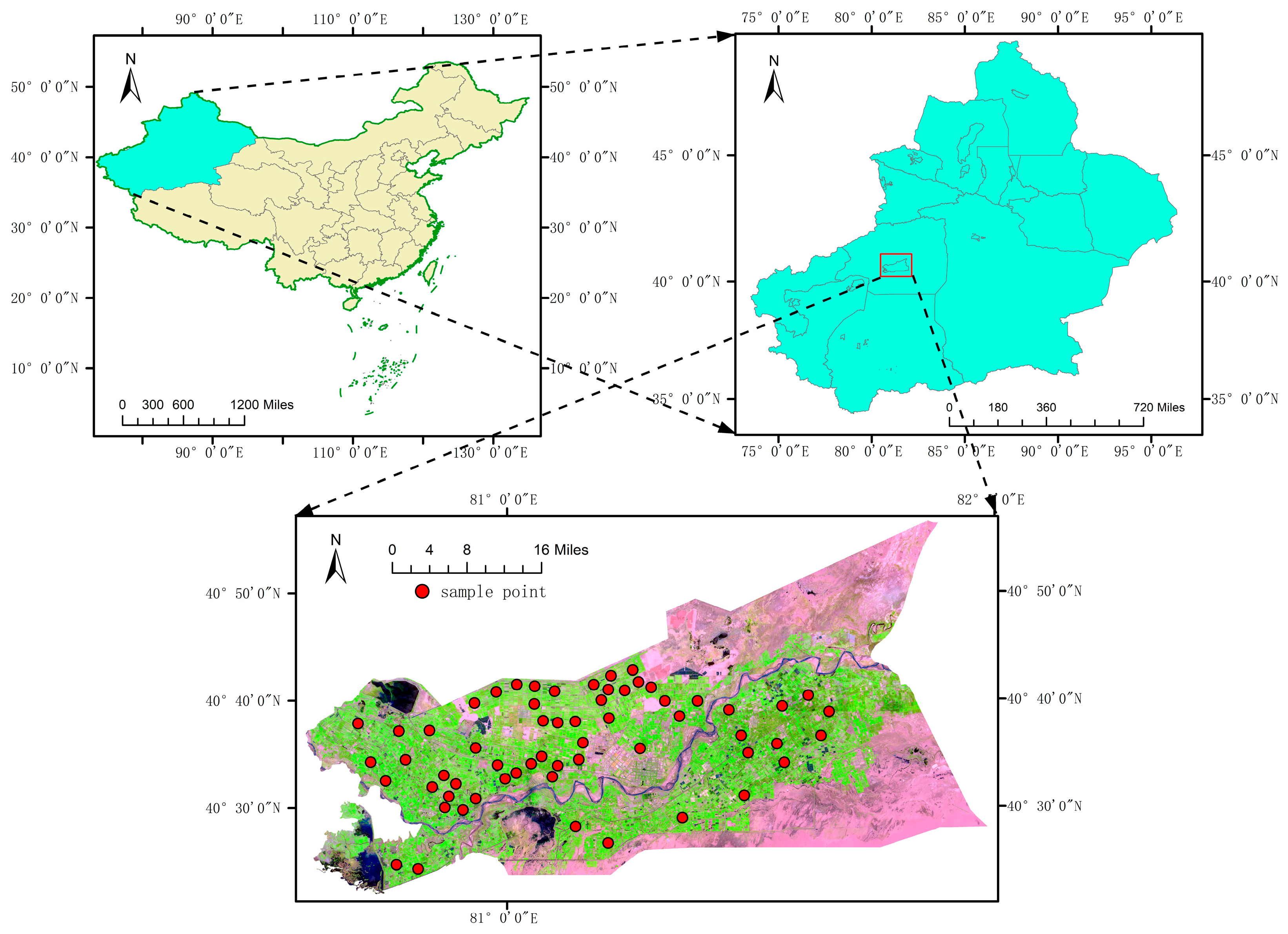
2.1. Overview of the Study Area

The study area is located in Alar City, the First Division of the Xinjiang Production and Construction Corps, with a total area of 6923.4 square kilometers. Geographically, it spans from 80°30′ to 81°58′ E longitude and from 40°22′ to 40°57′ N latitude. The region is bordered to the north by the southern foothills of the Tianshan Mountains, to the south by the northern edge of the Taklamakan Desert, to the east by Shaya County, and to the west by Keping County. This area is characterized by a warm, temperate, extremely continental, arid desert climate, with an average annual temperature of 10.7 °C, a frost-free period of 220 days, and an annual average sunshine duration of over 2900 h. Precipitation is scarce, with annual rainfall ranging from 40.1 mm to 82.5 mm, and annual evaporation varies between 1876.6 mm and 2558.9 mm. The region enjoys ample sunlight, making it favorable for the growth of fragrant pears. Due to its proximity to the desert, the climate is arid, and the water required for pear tree growth is primarily supplied through irrigation. This experiment was conducted from April to September 2024, covering the four key growth stages of fragrant pears: flowering (23 April), fruit-setting (28 May), fruit enlargement (7 July), and maturity (20 September). To ensure the representativeness of experimental samples, 60 standardized pear tree plots were selected within the study area. The pear trees within these plots were uniform in cultivar, age, and cultivation management practices. This experimental design enables a comprehensive characterization of the growth patterns of Pyrus sinkiangensis across different phenological stages, thereby providing a robust data foundation for the study. The geographical location of the study area is shown in Figure 1.

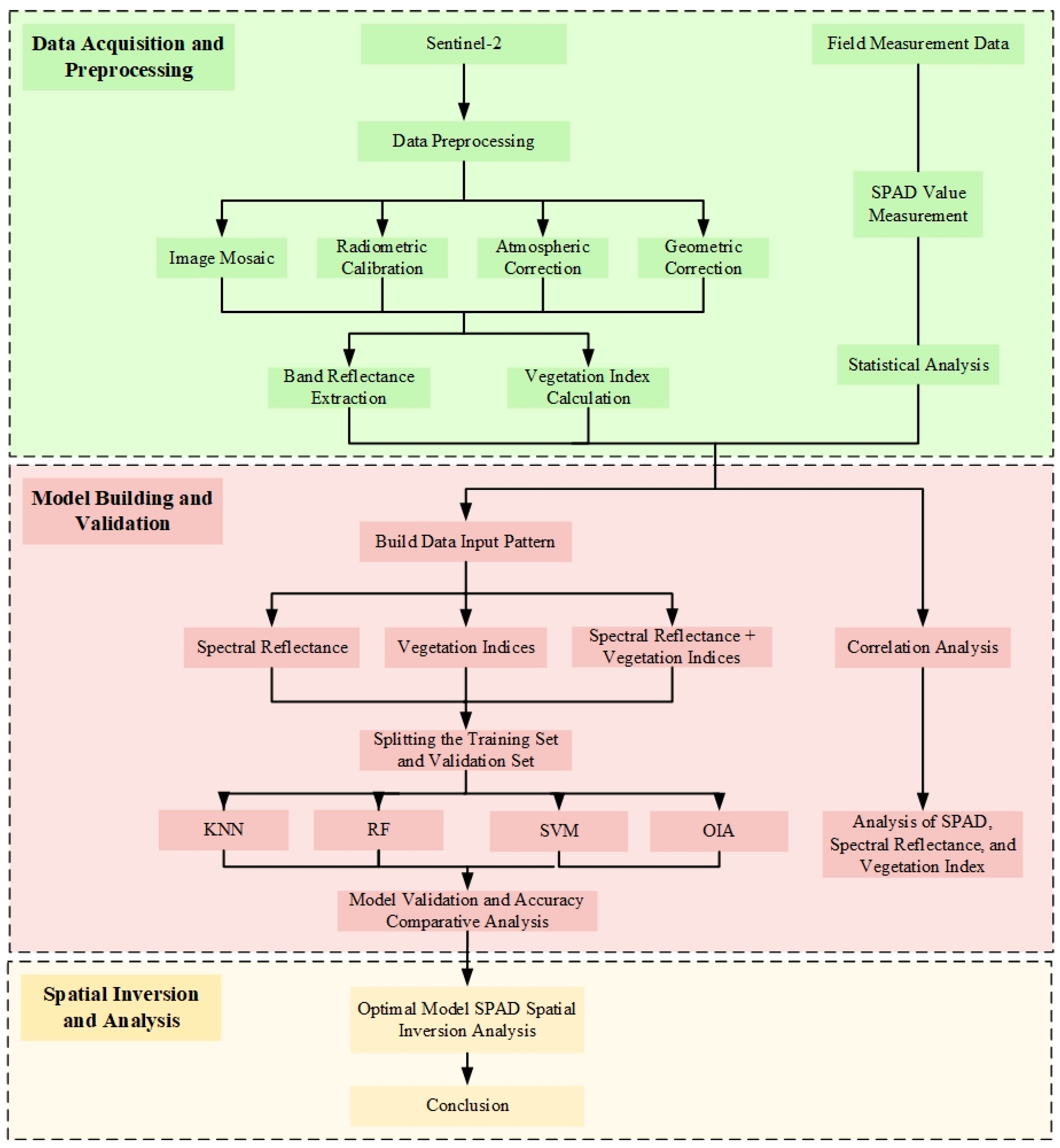
2.2. Data Acquisition and Processing

2.2.1. Remote Sensing Image Acquisition and Pre-Processing

This study primarily utilizes multispectral imagery from the Sentinel-2 satellite, developed by the European Space Agency (ESA), headquartered in Paris, France [27]. The satellite is equipped with a Multispectral Instrument (MSI) manufactured by Airbus Defence and Space, located in Ottobrunn, Germany. It features a 290 km swath width and a 5-day revisit cycle, providing data across 13 spectral bands, with a spatial resolution of up to 10 m in the visible bands. To accurately capture the spectral characteristics of pear tree canopies, imagery was selected based on the phenological characteristics of pear trees in the Alar reclamation area, in conjunction with the satellite’s revisit cycle. Specifically, images from four key growth stages—23 April 2024 (flowering), 28 May 2024 (fruit-setting), 7 July 2024 (fruit enlargement), and 20 September 2024 (maturity)—were chosen. Data acquisition was conducted via the ESA’s Science Data Hub https://dataspace.copernicus.eu (accessed on 23 April 2025) and the United States Geological Survey (USGS) platform. The data included two scenes of L1C-level imagery and four scenes of L2A-level imagery, where L2A images have been pre-processed to atmospheric bottom-of-atmosphere reflectance products, directly usable for band synthesis and area-of-interest clipping. The L1C images required additional preprocessing using the ESA’s Sen2Cor 2.09.00 plugin for radiometric calibration and atmospheric correction.

Given that Sentinel-2 imagery contains bands with spatial resolutions of 10 m, 20 m, and 60 m, this study performed spatial resampling to ensure consistency across all bands and alignment with the field plot scale. The Sentinel Application Platform (SNAP), officially provided by ESA, was used for image preprocessing. Specifically, the “Resampling” module was applied to resample the 20 m and 60 m bands to a uniform spatial resolution of 10 m using bilinear interpolation, which balances spatial accuracy and spectral continuity. To minimize potential spectral distortion introduced during resampling, only bands with acceptable mean error after resampling were retained. As the 60 m bands tend to exhibit higher spatial interpolation errors when resampled to 10 m and are primarily intended for atmospheric correction and cloud detection, bands B1 (443 nm), B9 (945 nm), and B10 (1375 nm) were excluded from model construction. Ultimately, 10 key bands with consistent 10 m resolution were selected as input variables: B2 (blue, 490 nm), B3 (green, 560 nm), B4 (red, 665 nm), B5 (red edge 1, 705 nm), B6 (red edge 2, 740 nm), B7 (red edge 3, 783 nm), B8 (broad NIR, 842 nm), B8A (narrow NIR, 865 nm), B11 (SWIR 1, 1610 nm), and B12 (SWIR 2, 2190 nm). For spatial registration between field sample data and remote sensing imagery, geometric correction was performed using high-precision ground control points (GCPs). A handheld RTK device with centimeter-level accuracy was used to collect geospatial coordinates of standard white reference boards placed within the sample plots. The acquired GCPs were then imported into ENVI 5.6, and a second-order polynomial correction model was applied for geometric refinement. To ensure registration accuracy, the results were quantitatively validated by calculating the root mean square error (RMSE) of the GCPs. The RMSE values were all below 3.5 m, well within the 10 m spatial resolution threshold, indicating sub-pixel registration accuracy. This high-precision spatial alignment effectively eliminated geolocation errors and provided a reliable geospatial foundation for subsequent quantitative retrieval, thereby significantly enhancing the accuracy and robustness of the inversion models.

2.2.2. Ground-Truthing Data Acquisition

In this study, the pear trees in the Alar reclamation area were selected as the research object. A systematic sampling method was employed to choose 60 representative sampling sites, with their spatial distribution covering the major production teams of the First Division (Yishi) throughout the region, ensuring the spatial representativeness of the research samples. To ensure the temporal consistency between the ground-measured SPAD values and the Sentinel-2 satellite imagery data, the sampling was strictly conducted within the satellite overpass time window. Specifically, based on the orbital cycle and overpass timing of the Sentinel-2 satellite (typically around 11:00 AM ± 15 min Beijing time for the Alar region), the research team accessed the planned acquisition schedule of target imagery in advance via the ESA Copernicus Open Access Hub. Observation plans were formulated three days prior to each acquisition, taking local weather forecasts into account. On the actual sampling days, ground-based SPAD measurements were conducted between 9:30 and 11:00 AM to ensure stable leaf physiological conditions, an appropriate solar elevation angle, and maximum temporal alignment with the satellite overpass. This protocol effectively minimized the influence of solar irradiance fluctuations and leaf water content variability on the inversion modeling process.

Based on the phenological characteristics of pear trees and taking into account the weather conditions on the day of the experiment, four key growth stages were selected for synchronized observations: flowering stage (23 April), fruit-setting stage (28 May), fruit enlargement stage (7 July), and maturity stage (20 September). A SPAD-502Plus chlorophyll meter was used to measure the SPAD values of the leaves. In each sampling site, ten representative pear trees with good growth conditions were randomly selected as observation samples. For each sampled tree, standardized sampling methods were applied: two healthy, mature leaves were chosen from each of the east, south, west, north, and top positions of the canopy, totaling ten leaves per tree. Five SPAD measurements were taken for each leaf, with the average value used as the SPAD value for that leaf. The average SPAD value of the ten leaves was taken as the SPAD value for each individual pear tree. Finally, the arithmetic mean of the SPAD values from the ten sampled trees in each sampling site was used as the representative value for that site. By implementing a multi-level data quality control protocol, the measurement scheme significantly enhanced the accuracy and reliability of ground-based observations, thereby providing a robust data foundation for the development of remote sensing inversion models and subsequent spatiotemporal analyses.

2.2.3. Vegetation Indices Selection and Calculation

Vegetation indices, as crucial indicators of vegetation growth status, play a key role in the inversion models of vegetation physiological parameters [28]. Building upon previous research, this study selected ten typical vegetation indices significantly correlated with vegetation chlorophyll content. These include the Normalized Difference Vegetation Index (NDVI), the Normalized Difference Red Edge Index (NDRE), the Ratio Vegetation Index (RVI), the Difference Vegetation Index (DVI), the Modified Chlorophyll Absorption Ratio Index (MCARI), the Optimized Soil-Adjusted Vegetation Index (OSAVI), the Chlorophyll Index (CI), the Soil-Adjusted Vegetation Index (SAVI), the Structure-Insensitive Pigment Index (SIPI), and the Enhanced Vegetation Index (EVI). These indices have wide-ranging applications in the field of crop growth monitoring. In this study, the geographic coordinates of sampling points were obtained using GPS and spatially registered with the corresponding remote sensing imagery. Spectral reflectance values of the matched pixels were then extracted and used to calculate multiple vegetation indices. These spectral metrics served as key feature variables for constructing remote sensing inversion models of SPAD values in pear tree leaves. The vegetation indices and their corresponding formulas are summarized in

Table 1. Vegetation indices and formula.

Vegetation Index	Calculation Formula	Reference
$\mathrm{N}\mathrm{D}\mathrm{V}\mathrm{I}$	$\mathrm{N}\mathrm{D}\mathrm{V}\mathrm{I}=(\mathrm{B}8-\mathrm{B}4)/(\mathrm{B}8+\mathrm{B}4)$	[29]
$\mathrm{N}\mathrm{D}\mathrm{R}\mathrm{E}$	$\mathrm{N}\mathrm{D}\mathrm{R}\mathrm{E}=(\mathrm{B}8-\mathrm{B}6)/(\mathrm{B}8+\mathrm{B}6)$	[29]
$\mathrm{R}\mathrm{V}\mathrm{I}$	$\mathrm{R}\mathrm{V}\mathrm{I}=\mathrm{B}8/\mathrm{B}4$	[30]
$\mathrm{D}\mathrm{V}\mathrm{R}$	$\mathrm{D}\mathrm{V}\mathrm{I}=\mathrm{B}8-\mathrm{B}4$	[30]
$\mathrm{M}\mathrm{C}\mathrm{A}\mathrm{R}\mathrm{I}$	$\mathrm{M}\mathrm{C}\mathrm{A}\mathrm{R}\mathrm{I}=[\left(\mathrm{B}5-\mathrm{B}4\right)-0.2\ast \left(\mathrm{B}5-\mathrm{B}3\right)]\ast \left({\displaystyle \frac{\mathrm{B}5}{\mathrm{B}4}}\right)$	[29]
$\mathrm{O}\mathrm{S}\mathrm{A}\mathrm{V}\mathrm{I}$	$\mathrm{O}\mathrm{S}\mathrm{A}\mathrm{V}\mathrm{I}=1.16\ast (\mathrm{B}8-\mathrm{B}4)/(\mathrm{B}8+\mathrm{B}4+0.16)$	[30]
$\mathrm{C}\mathrm{I}$	$\mathrm{C}\mathrm{I}=\left({\displaystyle \frac{\mathrm{B}8}{B3}}\right)-1$	[29]
$\mathrm{S}\mathrm{A}\mathrm{V}\mathrm{I}$	$\mathrm{S}\mathrm{A}\mathrm{V}\mathrm{I}=\left(1+\mathrm{L}\right)\ast (\mathrm{B}8-\mathrm{B}4)/(\mathrm{B}8+\mathrm{B}4+\mathrm{L})$	[30]
$\mathrm{S}\mathrm{I}\mathrm{P}\mathrm{I}$	$\mathrm{S}\mathrm{I}\mathrm{P}\mathrm{I}=(\mathrm{B}8-\mathrm{B}2)/(\mathrm{B}8-\mathrm{B}4)$	[31]
$\mathrm{E}\mathrm{V}\mathrm{I}$	$\mathrm{E}\mathrm{V}\mathrm{I}=2.5\ast (\mathrm{B}8-\mathrm{B}4)/(\mathrm{B}8+6\ast \mathrm{B}4-7.5\ast \mathrm{B}2+1)$	[32]

Note: For the wavelength ranges and detailed descriptions of bands B2, B3, B4, etc., please refer to Section 2.2.1.

.

2.3. Model Construction and Evaluation

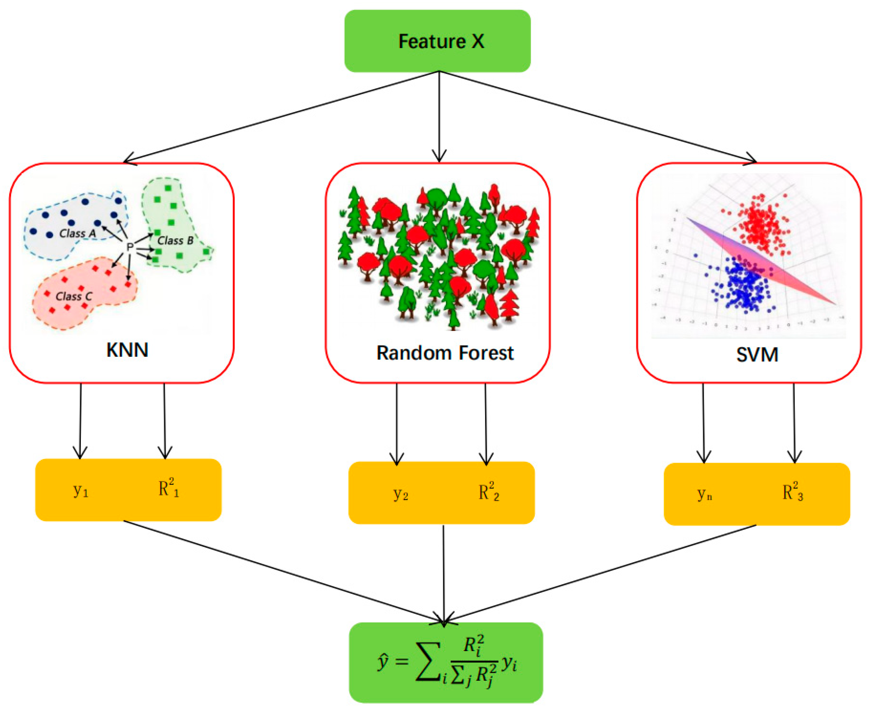
2.3.1. Model Construction Method

In the construction of remote sensing-based inversion models for SPAD values in pear leaves, this study utilized a total of 60 valid ground samples and adopted a five-fold cross-validation approach to evaluate model performance. Specifically, the entire dataset was evenly partitioned into five subsets. In each iteration, one subset was designated as the validation set, while the remaining four were used for model training. This process was repeated five times, and the average performance across all folds was taken as the final evaluation metric, thereby enhancing the stability and reliability of model assessment under limited sample conditions. Regarding input variable construction, three feature combination schemes were designed: (1) spectral reflectance only, (2) vegetation indices only, and (3) a combination of spectral reflectance and vegetation indices. For each input configuration, four machine learning models were developed: KNN, RF, SVM, and OIA. A systematic comparison of model performance was conducted across different phenological stages, and the best-performing model under each scenario was ultimately selected for SPAD inversion analysis. The overall technical workflow is illustrated in Figure 2.

(1) K-Nearest Neighbor (KNN) Algorithm

The K-Nearest Neighbor (KNN) algorithm is a fundamental classification and regression technique. The core principle is that if a sample belongs to the majority class among the K most similar (i.e., nearest in feature space) samples, the sample is classified into that class. In classification problems, assuming each point in feature space has a class label, the task is to determine the class of a new sample point x. This involves calculating the distance between x and all training samples, typically using the Euclidean distance formula:

$$d\left(x,y\right)=\sqrt{{\sum }_{i=1}^n{\left(x_i-y_i\right)}^2}$$

(1)

where x = (x₁, x₂, …, x_n), and y = (y₁, y₂, …, y_n) are the feature vectors of two sample points, and n is the number of features. The K nearest neighbors are identified, and the class with the highest frequency among them is assigned to x. In regression tasks, the average target value of the K nearest neighbors is typically used as the predicted value. The KNN algorithm in this study was selected to predict the SPAD values of unknown samples by calculating the spectral distance between the sample to be inverted and the training samples, thereby leveraging the SPAD data of known samples to predict the SPAD value of unknown samples, fully utilizing the information contained in the spectral data related to pear tree leaf SPAD values.

(2) Random Forest Algorithm

Random Forest is an ensemble learning algorithm based on decision trees [33]. It constructs multiple decision trees by randomly sampling the original training dataset with replacement and then combines the predictions from these trees to make the final decision. In classification tasks, the most frequent class among the predictions is chosen as the final class; in regression tasks, the average of the predictions from all decision trees is taken as the final value. The Random Forest algorithm effectively reduces the model’s variance, enhances its generalization ability, and exhibits good robustness to noisy data and overfitting. Additionally, it can handle high-dimensional data without excessive feature selection. The prediction of a Random Forest model can be expressed as

$$\widehat{Y}={\displaystyle \frac{1}{N_t}}{\sum }_{i=1}^{N_t}{f}_i\left(x\right)$$

(2)

where $\widehat{Y}$ is the final predicted result, $N_t$ is the number of decision trees, and $f_i\left(x\right)$ is the prediction from the i-th decision tree for input sample x. Random Forest improves model diversity through random sampling and feature-selection mechanisms, reducing model variance and mitigating the risk of overfitting, thus demonstrating robust performance even with small training datasets.

(3) Support Vector Machine (SVM) Algorithm

Support Vector Machine (SVM) is a machine learning algorithm based on statistical learning theory [34]. The core concept of SVM is to construct the optimal separating hyperplane that maximizes the margin between positive and negative samples, with the aim of minimizing the total deviation of all sample points from the hyperplane. As an extension of SVM, Support Vector Regression (SVR) seeks to find the optimal regression hyperplane, minimizing the total deviation of all sample points from the hyperplane. SVM shows excellent potential in estimation due to its versatility, robustness, and effectiveness, capable of handling high-dimensional and nonlinear data and exhibiting strong generalization ability. In this study, the SVM algorithm was implemented using the Support Vector Regression function in the Scikit-Learn (0.21.3) package within the Python 3.9 environment. The performance of the SVM model was influenced by parameters such as the loss function (Gamma), error penalty factor C, and kernel function. The radial basis function (RBF) kernel was chosen, with C = 1.0, and $\mathsf{\gamma }={\displaystyle \frac{1}{nfeatures}}$.

(4) Optimized Integrated Algorithm (OIA)

The Optimized Integrated Algorithm (OIA), as an advanced machine learning technique, aims to construct a predictive model with enhanced performance and generalization ability by organically integrating multiple base learners. This method leverages the complementary strengths of different base models and employs various ensemble strategies to effectively aggregate their predictions, thereby significantly improving overall accuracy. The core of the OIA approach lies in the diversity among base models. By tuning model parameters and selecting relevant features, the performance of individual learners can be optimized, enhancing the expressive capacity of the ensemble model. This strategy not only reduces the risk of overfitting but also significantly improves the model’s generalization ability when dealing with complex, nonlinear, or high-dimensional data. In practice, OIA often demonstrates superior stability and adaptability compared to single-model approaches, making it highly effective for solving challenging remote sensing estimation problems.

To further improve the robustness and generalizability of model evaluation, a five-fold cross-validation strategy was incorporated into the OIA model construction process. The OIA framework in this study integrates three representative machine learning algorithms—KNN, RF, and SVM—as base learners and employs a weighted ensemble mechanism, as illustrated in Figure 3. Specifically, each base model (KNN, RF, and SVM) was independently trained and used to predict SPAD values on the validation subsets. Performance metrics were then calculated for each model and normalized to derive standardized weight coefficients. Finally, the outputs from the three models were combined using a linear weighted fusion scheme to generate the optimized predictions, achieving high-accuracy SPAD inversion of pear leaves from remote sensing data. This ensemble strategy not only improved prediction accuracy but also enhanced model robustness under different data partitioning scenarios. It proved particularly effective for remote sensing applications characterized by small sample sizes, high dimensionality, and strong nonlinearity.

2.3.2. Evaluation of Model Accuracy

This study employs the coefficient of determination (R²), root mean square error (RMSE), and mean absolute error (MAE) to evaluate the model accuracy. R² is used to assess the degree of fit between the predicted and observed values, with values closer to 1 indicating better model fit. MAE and RMSE are commonly used metrics for measuring the deviation between predicted and actual observed values. They reflect the accuracy of the model’s predictions, with lower values indicating a higher model fit and better predictive performance. The specific calculation formulas are provided in Equations (3)–(5).

$$R^2=1-{\displaystyle \frac{{\sum }_{i=1}^n{\left(y_i-{\widehat{y}}_i\right)}^2}{{\sum }_{i=1}^n{\left(y_i-\overline{y}\right)}^2}}$$

(3)

$$RMSE=\sqrt{{\displaystyle \frac{{\sum }_{i=1}^n({y_i-{\widehat{y}}_i)}^2}{n}}}$$

(4)

$$MAE={\displaystyle \frac{1}{n}}{\sum }_{i=1}^n\left|y_i-{\widehat{y}}_i\right|$$

(5)

In the formula, n represents the number of samples, $y_i$ denotes the observed value of the i-th sample, ${\widehat{y}}_i$ is the corresponding predicted value, and $\overline{y}$ is the mean of the observed values.

In this study, the Pearson correlation coefficient (r) was employed to quantitatively assess the linear relationships between the SPAD values of pear tree leaves and both spectral reflectance across different bands and various vegetation indices. As shown in

Table 2. Variable relevance assessment via correlation coefficients.

Correlation Coefficient	Relevant Intensity
0.0–0.2	Very weak correlation or no correlation
0.2–0.4	Weak correlation
0.4–0.6	Moderately relevant
0.6–0.8	Strong correlation
0.8–1.0	Highly relevant

, vegetation indices with absolute correlation coefficients greater than 0.6 and spectral bands with coefficients exceeding 0.5 were selected at each of the four phenological stages as feature variables for subsequent SPAD inversion model development. This feature selection strategy effectively retains spectral characteristics that exhibit statistically significant associations with SPAD values, while minimizing the impact of irrelevant variables on model performance.

$$\mathrm{r}={\displaystyle \frac{{\left[\sum _{i=1}^n\left(x_i-\overline{x}\right)\left(y_i-\overline{y}\right)\right]}^2}{\sum _{i=1}^n{\left(x_i-\overline{x}\right)}^2\sum _{i=1}^n{\left(y_i-\overline{y}\right)}^2}}$$

(6)

3. Results

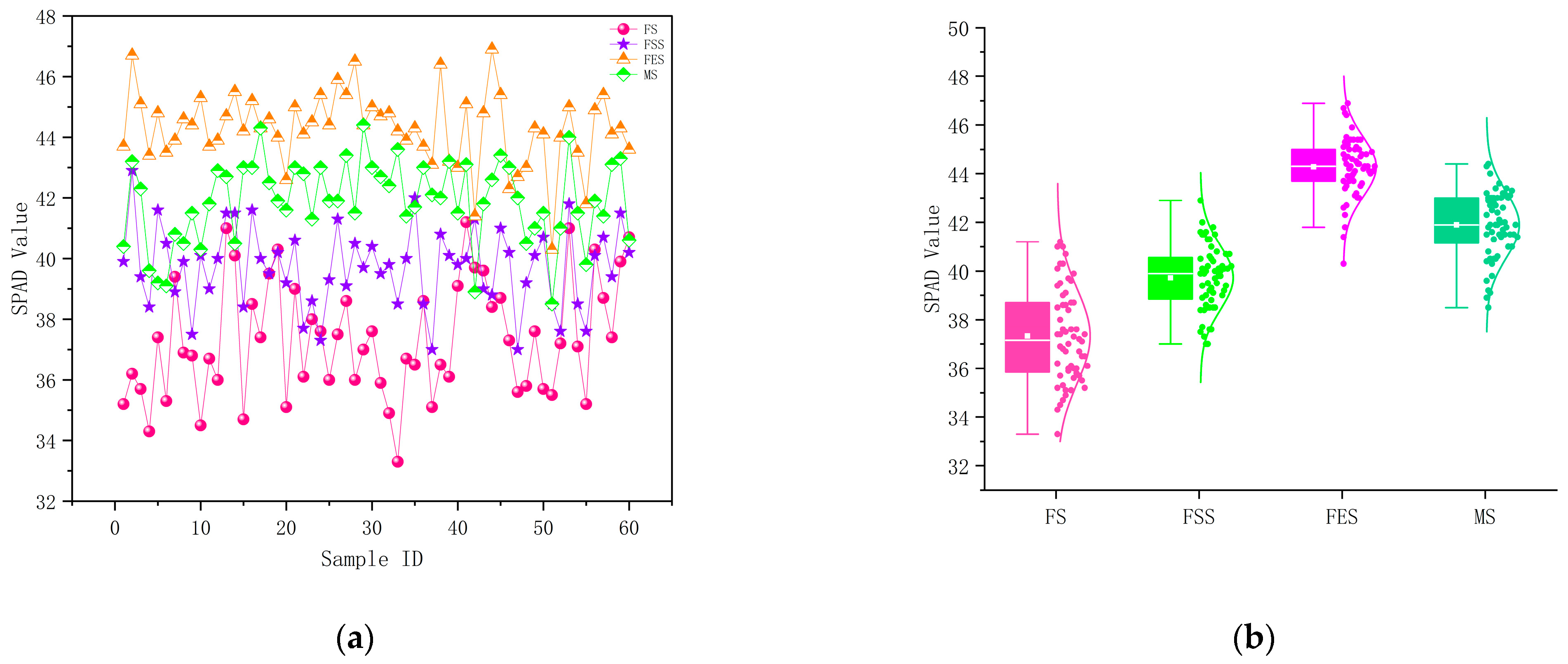
3.1. Variation Characteristics of SPAD Values of Pear Tree Leaves

The dynamic changes in SPAD values of pear tree leaves at different growth stages are illustrated in Figure 4. As shown in the figure, the SPAD values of pear tree leaves varied between 33.3 and 46.9 across the four growth stages in this study. During the flowering stage, the mean SPAD value was 37.3, with a standard deviation of 2.13 and a coefficient of variation (CV) of 5.36%. During the fruit-setting stage, the average SPAD value was 39.9, with a standard deviation of 1.42 and a CV of 3.56%. The fruit enlargement stage had a mean SPAD value of 44.3, with a standard deviation of 1.57 and a CV of 3.52%. Finally, during the maturity stage, the mean SPAD value was 41.9, with a standard deviation of 1.52 and a CV of 3.65%, exhibiting significant differences across growth stages (p < 0.05). From flowering to maturity, the SPAD values followed a unimodal pattern, first increasing and then decreasing, peaking at 46.9 ± 1.65 during the fruit enlargement stage. This trend is closely related to the physiological characteristics of pear tree growth: during the vegetative growth phase (from flowering to fruit enlargement), leaves enhance photosynthesis to accumulate assimilates, leading to continuous increases in chlorophyll content; whereas during the reproductive growth phase (from fruit enlargement to maturity), assimilates are transferred to the fruit, causing the leaves to enter a senescence phase, where chlorophyll gradually degrades, resulting in a decline in SPAD values. The coefficient of variation analysis of SPAD values across growth stages (

Table 3. Statistics of SPAD values of pear tree leaves at different growth stages.

Growth Period	Sample Size	SPAD Minimum Value	SPAD Maximum Value	SPAD Average Value	Standard Deviation	Coefficient of Variation
Flowering Stage	60	33.3	41.2	37.3	2.13	5.36%
Fruit-Setting Stage	60	37	42.9	39.9	1.42	3.56%
Fruit Enlargement Stage	60	40.3	46.9	44.3	1.57	3.52%
Maturity Stage	60	38.5	44.4	41.9	1.52	3.65%

) revealed that the flowering stage exhibited the highest CV (5.36%), while the CVs for subsequent growth stages remained stable between 3.52% and 3.65%. The CVs for all growth stages were below 6%, indicating a high level of stability in SPAD values among the samples. This suggests favorable conditions for establishing a unified nutritional diagnosis standard. The relatively small variation in SPAD values may be attributed to the standardized sampling methods and management practices employed during the experiment.

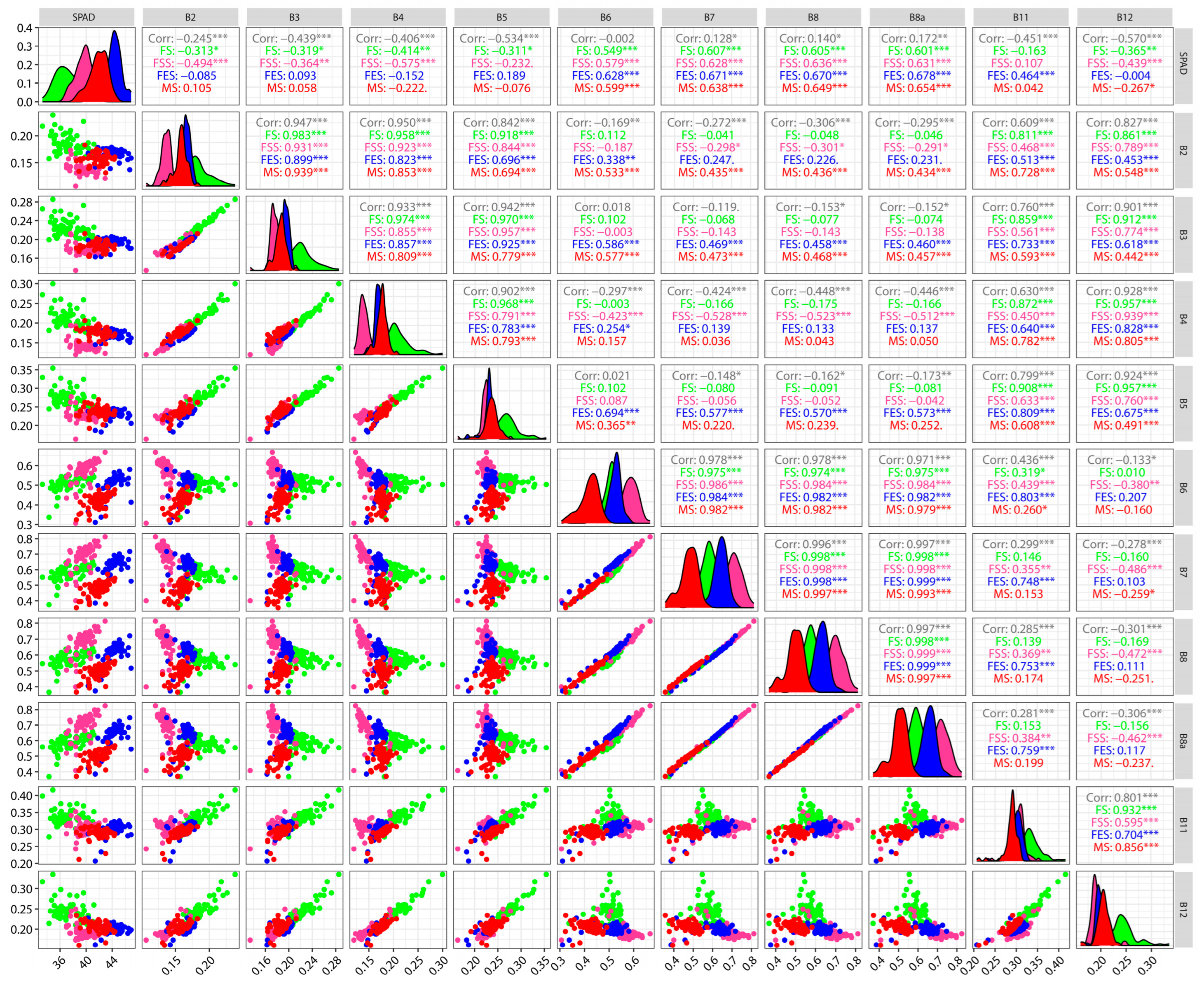
3.2. Analysis of SPAD Values and Spectral Reflectance Characteristics

As the phenological stages progress, the canopy structure, leaf coverage, and internal physiological parameters of pear trees undergo continuous changes, leading to distinct stage-specific variations in canopy spectral characteristics. To further analyze the spectral response features of pear canopies across different growth stages, this study selected four representative sample plots, each corresponding to a phenological stage and having SPAD values closest to the stage’s average field measurement. The selected plots were flowering stage (Sample ID.46, SPAD = 37.3), fruit-setting stage (Sample ID.32, SPAD = 39.9), fruit expansion stage (Sample ID.35, SPAD = 44.3), and maturity stage (Sample ID.57, SPAD = 41.9). Surface reflectance data for these plots were extracted from Sentinel-2 multispectral imagery, and a comparative analysis of canopy spectral characteristics across the four stages was conducted, as shown in Figure 5. The analysis revealed significant differences in spectral reflectance across phenological stages. In the visible bands (B2–B4), the highest reflectance was observed during the flowering stage, indicating lower green leaf coverage and greater spectral interference from flowers and bare soil background. As the growth progressed, leaf density increased and the canopy gradually closed, resulting in decreased reflectance, reaching its lowest level during the fruit expansion stage—reflecting peak chlorophyll content and photosynthetic activity. The red-edge and near-infrared bands (B5–B8A), known for their sensitivity to canopy structure, exhibited the highest reflectance and steepest spectral rise during the fruit expansion stage, indicating a dense and intact leaf structure with strong spectral responses. In contrast, reflectance during the flowering and fruit-setting stages remained relatively low, suggesting that the canopy structure was not yet well developed. In the shortwave infrared bands (B11–B12), the lowest reflectance occurred during the fruit expansion stage, implying the highest leaf water content and strongest physiological activity of the canopy. Overall, the fruit expansion stage exhibited the most stable reflectance characteristics, with the most continuous and distinct spectral curves, which is advantageous for improving the accuracy of inversion models.

3.3. Correlation Analysis Between Spectral Reflectance and SPAD Values

The results of the correlation analysis between spectral reflectance and SPAD values for pear trees at different growth stages are shown in Figure 6. A comparison of the performance of various spectral variables across the four growth stages of pear trees reveals a distinct pattern in the spectral reflectance. The correlation between spectral reflectance from the B6 and B7 red-edge bands, as well as the B8 and B8a near-infrared bands, and the observed SPAD values reached a highly significant level of 0.001, with the B8a band showing relatively better performance. Notably, as the growth stages progressed, the correlation between these bands and SPAD values improved. The correlation between spectral reflectance and SPAD values varied across different growth stages, with the order of correlation strength being fruit enlargement > maturity > fruit-setting > flowering. The highest correlation coefficient was observed during the fruit enlargement stage, where pear trees were in the later stages of reproductive growth, chlorophyll content peaked, and the canopy reflectance was less influenced by external factors, thus enhancing the correlation between spectral reflectance and SPAD values. It is worth noting that the correlation coefficient for the overall sample was not as strong as for individual growth stages. This is primarily due to significant physiological differences between growth stages, with leaves at different stages responding differently to the same spectral bands. These differences, when combined in the overall sample, obscure the more stable relationship between SPAD values and spectral reflectance at each individual growth stage, leading to a lower correlation coefficient for the overall sample. Considering the higher correlation performance of the B6, B7, B8, and B8a bands across all four growth stages, these bands were selected for inclusion in subsequent modeling. This approach aims to construct more accurate models for pear tree growth monitoring and management, providing a solid scientific foundation for further research.

3.4. Correlation Analysis Between Vegetation Indices and SPAD Values

The correlation analysis between vegetation indices and SPAD values across different phenological stages of pear trees (Figure 7) indicates significant variations in the relationship between vegetation indices and SPAD values across growth stages. The results show that vegetation indices such as NDVI, RVI, DVI, OSAVI, CI, SAVI, and EVI exhibit significant positive correlations with SPAD values, with the most pronounced correlations observed during the swelling stage. Specifically, the correlation coefficient for NDVI reaches 0.723 during the swelling stage, while RVI has a correlation coefficient of 0.719 during the same period, indicating that these indices are highly sensitive to changes in SPAD values. Notably, as the growth cycle progresses, the correlation first increases and then decreases, with the correlation generally weakening during the maturity stage. The study also found that the SIPI index showed a significant negative correlation with SPAD values throughout all growth stages, with the strongest negative correlation observed during the flowering and maturity stages. This phenomenon may reflect the sensitivity of the SIPI index to the chlorophyll degradation process. In contrast, the NDRE and MCARI indices exhibited moderate correlations with SPAD values across all growth stages, suggesting that their applicability as monitoring indices for SPAD values is limited. Overall, the analysis demonstrates that the seven vegetation indices—NDVI, RVI, DVI, OSAVI, CI, SAVI, and EVI—perform well in monitoring SPAD values across different phenological stages of pear trees. These indices accurately reflect the dynamic changes in leaf chlorophyll content, especially during critical growth stages (FES and MS), providing reliable remote sensing indicators for monitoring pear tree growth. Based on these findings, the present study uses these seven vegetation indices to construct the SPAD inversion model.

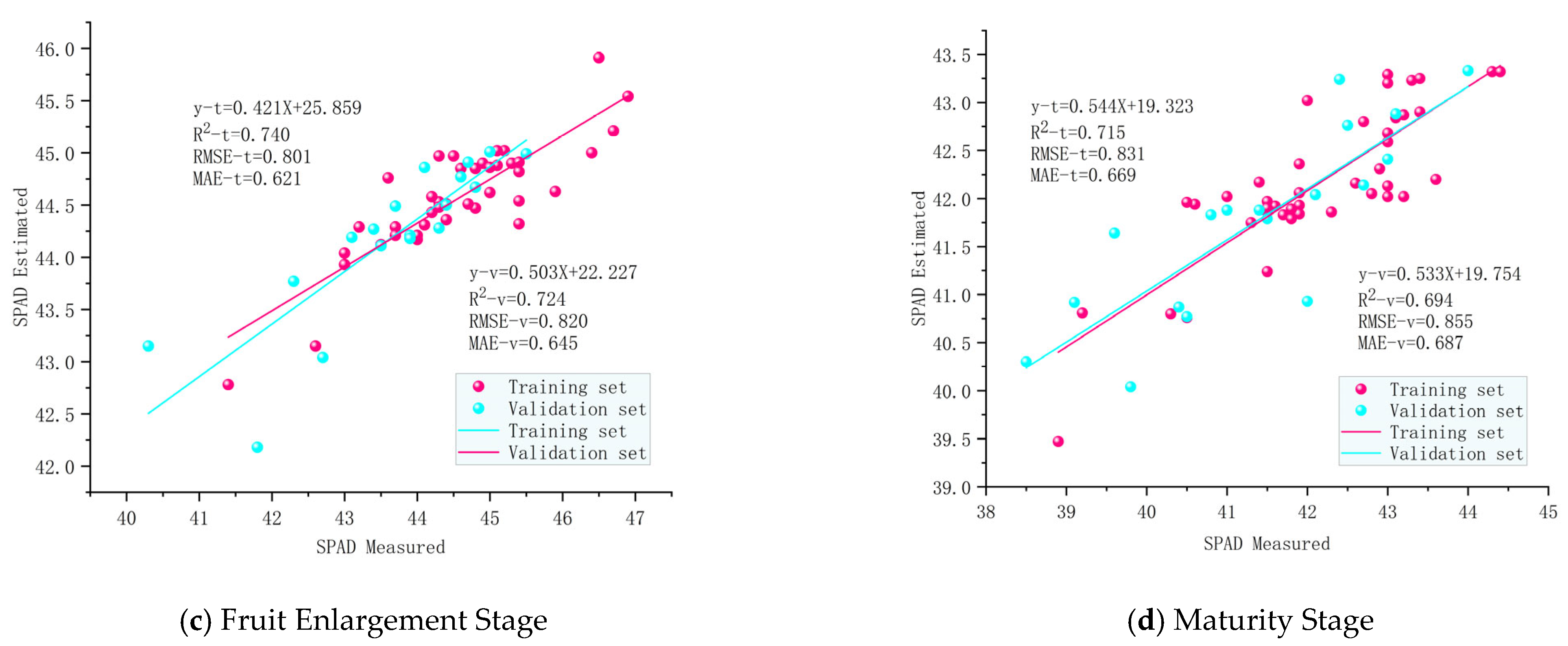
3.5. Inversion Model Results and Analysis for SPAD Values of Pear Tree Leaves

This study focuses on four key growth stages of pear trees: flowering, fruit-setting, fruit enlargement, and maturity. We developed SPAD value inversion models using three different input variable configurations—band reflectance alone, vegetation indices alone, and a combination of band reflectance and vegetation indices. Four representative machine learning algorithms—KNN, RF, SVM, OIA—were employed to construct these models. A comprehensive comparison and analysis of model performance across the different growth stages was carried out. At the flowering stage, the inversion results are presented in

Table 4. Summary of the inversion results during the flowering stage.

Model	Data Set	Spectral Reflectance				Vegetation Indices				Spectral Reflectance + Vegetation Indices
		R2	STD	RMSE	MAE	R2	STD	RMSE	MAE	R2	STD	RMSE	MAE
KNN	Training Set	0.596	0.039	1.195	0.993	0.631	0.035	1.096	0.939	0.650	0.037	1.079	0.863
	Validation Set	0.571	0.042	1.210	1.079	0.618	0.038	1.103	0.954	0.637	0.042	1.093	0.876
RF	Training Set	0.624	0.035	1.109	0.954	0.645	0.032	1.080	0.869	0.669	0.032	0.995	0.776
	Validation Set	0.597	0.038	1.148	0.993	0.632	0.034	1.101	0.940	0.650	0.035	1.085	0.867
SVM	Training Set	0.605	0.034	1.125	0.970	0.634	0.030	1.093	0.963	0.658	0.033	1.060	0.863
	Validation Set	0.591	0.040	1.157	1.041	0.626	0.035	1.110	0.956	0.646	0.037	1.087	0.875
OIA	Training Set	0.38	0.035	1.101	0.939	0.652	0.029	1.069	0.871	0.675	0.027	0.985	0.764
	Validation Set	0.615	0.031	1.110	0.953	0.638	0.031	1.107	0.942	0.663	0.028	0.995	0.774

. Among the models using a combination of band reflectance and vegetation indices as input variables, the OIA model exhibited the best performance. For the training dataset, the R² was 0.675, with an RMSE of 0.985 and an MAE of 0.764. For the validation dataset, R² reached 0.663, with RMSE and MAE values of 0.995 and 0.774, respectively. Compared to the OIA model using only band reflectance or vegetation indices as input, the combined model improved R² by 0.048 and 0.025 and reduced RMSE by 0.115 and 0.112 and MAE by 0.179 and 0.168 for the validation dataset. When compared to the other three algorithms (KNN, RF, and SVM) using the same combined input of band reflectance and vegetation indices, the OIA model outperformed them by increasing R² by 0.026, 0.013, and 0.017, respectively. Additionally, it reduced RMSE by 0.098, 0.090, and 0.092 and decreased MAE by 0.102, 0.093, and 0.101. Considering the standard deviation of the validation set R² (±0.028), the model maintained stable predictive performance across different data partitions, further confirming its superiority and generalization capability in SPAD value estimation.

In the SPAD value inversion for pear tree leaves during the fruit-setting stage, as summarized in

Table 5. Summary of the inversion results during the fruit-setting stage.

Model	Data Set	Spectral Reflectance				Vegetation Indices				Spectral Reflectance + Vegetation Indices
		R2	STD	RMSE	MAE	R2	STD	RMSE	MAE	R2	STD	RMSE	MAE
KNN	Training Set	0.616	0.035	1.105	0.966	0.647	0.040	1.078	0.861	0.657	0.027	1.065	0.867
	Validation Set	0.608	0.038	1.120	0.967	0.630	0.039	1.102	0.944	0.646	0.029	1.078	0.870
RF	Training Set	0.644	0.032	1.076	0.874	0.658	0.035	1.062	0.861	0.674	0.025	0.981	0.760
	Validation Set	0.632	0.036	1.097	0.944	0.646	0.037	1.081	0.863	0.663	0.026	0.995	0.786
SVM	Training Set	0.633	0.039	1.094	0.940	0.647	0.034	1.075	0.869	0.665	0.025	0.991	0.780
	Validation Set	0.621	0.042	1.101	0.948	0.635	0.041	1.095	0.966	0.650	0.028	1.076	0.858
OIA	Training Set	0.653	0.027	1.076	0.851	0.678	0.028	0.977	0.752	0.709	0.021	0.840	0.673
	Validation Set	0.645	0.029	1.089	0.877	0.657	0.030	1.062	0.861	0.685	0.024	0.901	0.702

, the OIA model again achieved the optimal results when using a combination of band reflectance and vegetation indices as input variables. For the training dataset, the R² was 0.709, with an RMSE of 0.840 and an MAE of 0.673. For the validation dataset, R² was 0.685, with RMSE and MAE values of 0.901 and 0.702, respectively. Compared to models using only band reflectance or vegetation indices as single input variables, the combined input model improved R² by 0.040 and 0.028 for the validation dataset, while RMSE and MAE were significantly reduced. In comparison with the KNN, RF, and SVM models, using the same combined input of band reflectance and vegetation indices, the OIA model outperformed them by increasing R² by 0.039, 0.022, and 0.035, respectively. Additionally, RMSE decreased by 0.177, 0.094, and 0.175, and MAE was reduced by 0.168, 0.084, and 0.156, indicating its greater robustness during this growth stage.

The fruit enlargement stage is a critical period for leaf physiological activity, and the accuracy of the inversion models further improves during this phase. The inversion results are summarized in

Table 6. Summary of the inversion results during the fruit enlargement stage.

Model	Data Set	Spectral Reflectance				Vegetation Indices				Spectral Reflectance + Vegetation Indices
		R2	STD	RMSE	MAE	R2	STD	RMSE	MAE	R2	STD	RMSE	MAE
KNN	Training Set	0.645	0.033	1.077	0.871	0.656	0.030	1.067	0.870	0.678	0.021	0.976	0.751
	Validation Set	0.627	0.036	1.110	0.956	0.638	0.032	1.110	0.928	0.654	0.025	1.067	0.848
RF	Training Set	0.654	0.031	1.067	0.864	0.669	0.029	0.985	0.771	0.684	0.019	0.899	0.701
	Validation Set	0.643	0.033	1.095	0.876	0.658	0.033	1.057	0.859	0.669	0.020	0.982	0.758
SVM	Training Set	0.649	0.035	1.081	0.856	0.659	0.028	1.060	0.861	0.676	0.022	0.980	0.757
	Validation Set	0.637	0.033	1.110	0.925	0.642	0.031	1.093	0.884	0.658	0.026	1.061	0.863
OIA	Training Set	0.684	0.026	0.904	0.705	0.704	0.026	0.843	0.675	0.740	0.016	0.801	0.621
	Validation Set	0.663	0.030	1.013	0.787	0.688	0.028	0.897	0.701	0.724	0.018	0.820	0.645

. Under the input condition of combined band reflectance and vegetation indices, the OIA model achieved an R² of 0.740, with an RMSE of 0.801 and an MAE of 0.621 for the training dataset. For the validation dataset, R² was 0.724, with RMSE and MAE values of 0.820 and 0.645, respectively. Overall, the OIA model outperformed the other models. Compared to the single-variable input models using only band reflectance or vegetation indices, the combined input model increased R² for the validation dataset by 0.061 and 0.036 and also showed significant reductions in RMSE and MAE. When compared to the KNN, RF, and SVM models using the same combined input of band reflectance and vegetation indices, the OIA model improved R² by 0.070, 0.055, and 0.066, respectively, for the validation dataset. Additionally, RMSE was reduced by 0.247, 0.162, and 0.241, and MAE decreased by 0.203, 0.113, and 0.218. Given the relatively small standard deviation of R² on the validation set (±0.018), the model demonstrated strong stability and generalization capability across different data partitions, highlighting its sensitive response and reliable adaptability to the spatiotemporal variation of SPAD values.

During the maturity stage of pear trees, although the overall model prediction accuracy slightly decreased, the OIA model maintained its leading position. The inversion results are summarized in

Table 7. Summary of the inversion results during the maturity stage.

Model	Data Set	Spectral Reflectance				Vegetation Indices				Spectral Reflectance + Vegetation Indices
		R2	STD	RMSE	MAE	R2	STD	RMSE	MAE	R2	STD	RMSE	MAE
KNN	Training Set	0.631	0.038	1.094	0.941	0.649	0.034	1.080	0.858	0.664	0.025	1.024	0.791
	Validation Set	0.622	0.039	1.100	0.961	0.634	0.037	1.097	0.943	0.646	0.028	1.073	0.867
RF	Training Set	0.651	0.033	1.080	0.849	0.659	0.031	1.062	0.865	0.675	0.024	0.977	0.760
	Validation Set	0.637	0.035	1.112	0.928	0.643	0.033	1.090	0.887	0.664	0.026	1.018	0.792
SVM	Training Set	0.641	0.034	1.094	0.922	0.652	0.029	1.073	0.850	0.665	0.025	1.010	0.787
	Validation Set	0.632	0.036	1.097	0.945	0.637	0.032	1.108	0.922	0.654	0.027	1.070	0.846
OIA	Training Set	0.671	0.029	0.980	0.751	0.695	0.029	0.852	0.660	0.715	0.020	0.831	0.669
	Validation Set	0.660	0.030	1.008	0.779	0.674	0.029	0.982	0.761	0.694	0.021	0.855	0.687

Note: Due to space limitations and common practices in remote sensing research, only the standard deviation of the R² mean is reported in Table 4, Table 5, Table 6 and Table 7 to reflect the model stability across different partitions.

. The model using a combination of band reflectance and vegetation indices as input achieved R² values of 0.715 and 0.694 for the training and validation datasets, respectively. The RMSE was 0.831 for the training dataset and 0.855 for the validation dataset, while the MAE was 0.669 and 0.687, respectively. Compared to the other three models, the OIA model demonstrated an improvement in R² for the validation dataset, with corresponding reductions in RMSE and MAE. These results indicate that, even during the late stage when vegetative activity slows, the OIA model still exhibits strong adaptability. Given the standard deviation of R² on the validation set (±0.021), the OIA model maintained good stability and generalization performance across different data partitions, indicating strong adaptability and robustness even during the later phenological stages when vegetation activity declines.

Based on the results above, the optimal models for SPAD value inversion of pear tree leaves at different growth stages were selected, as illustrated in Figure 8. Among the four machine learning methods, the OIA consistently exhibited the best predictive performance across all growth stages, making it the most effective modeling method for the inversion of pear tree leaf SPAD values. In terms of input variable selection, models using a combination of band reflectance and vegetation indices outperformed those with single-variable inputs in all growth stages. This suggests that integrating multi-source remote sensing features can significantly enhance model accuracy. Therefore, the OIA model with combined band reflectance and vegetation indices is identified as the optimal combination for SPAD value inversion across all growth stages. Further comparison of inversion performance across different growth stages revealed that the model for the fruit enlargement stage achieved the highest accuracy, followed by the maturity, fruit-setting, and flowering stages. This indicates that the SPAD values of leaves during the fruit enlargement stage are the most stable and less challenging to invert, providing a theoretical foundation and technical support for future monitoring and management strategies of pear tree nutritional status.

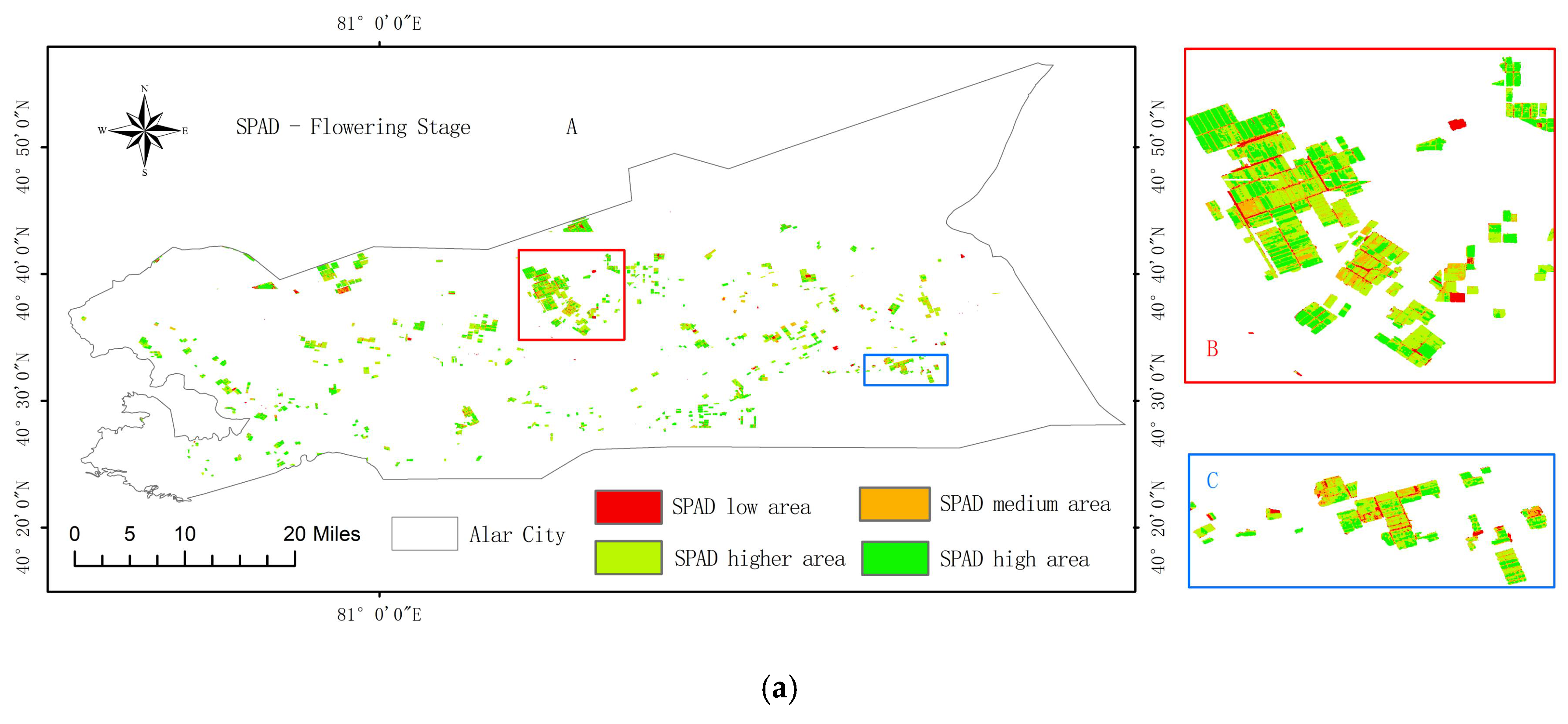
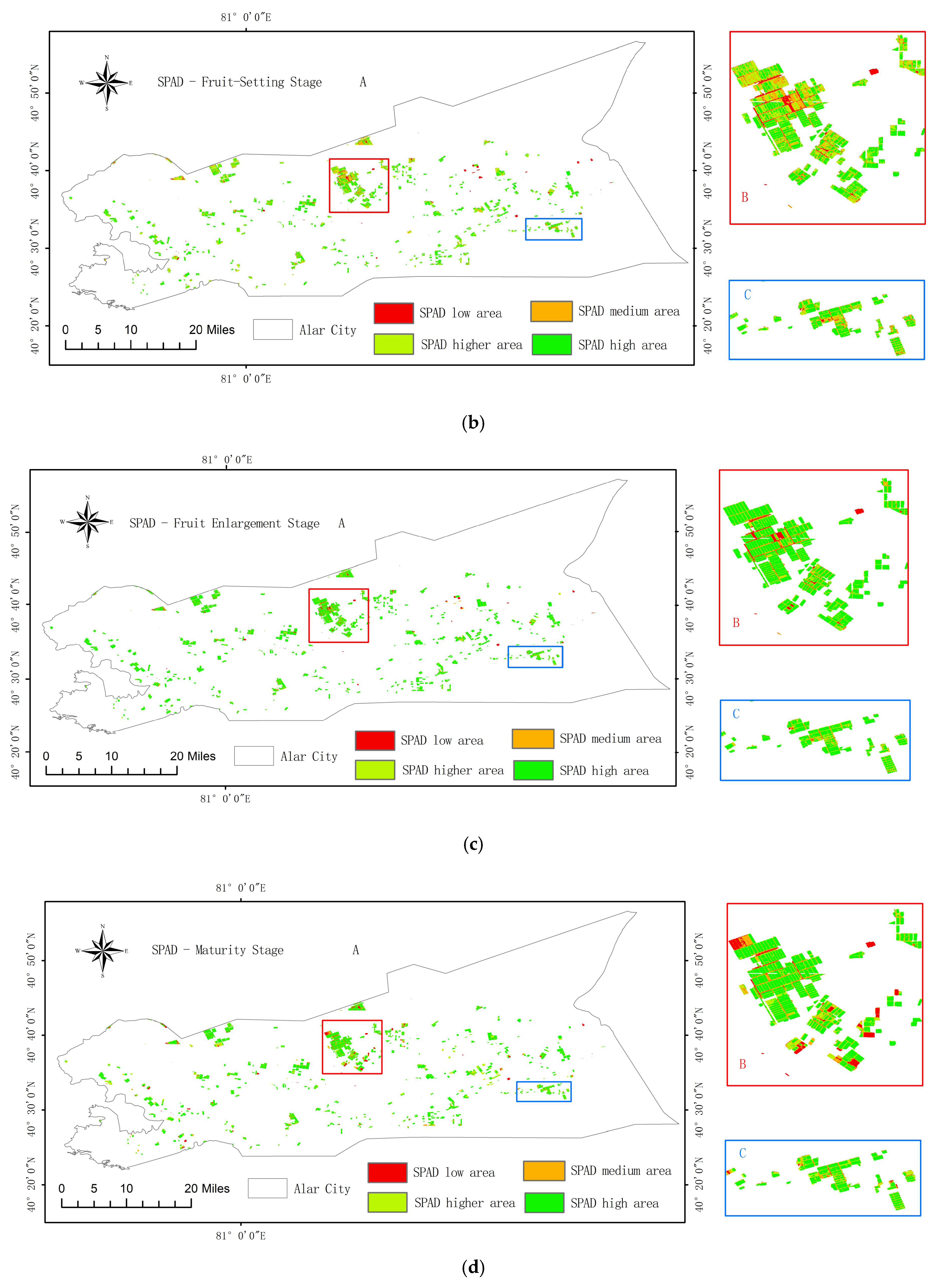
3.6. Temporal and Spatial Distribution Characteristics of Pear Tree Leaf SPAD Values Based on the Optimal Model

The optimal SPAD value inversion model developed in this study is the OIA model, which uses a combination of band reflectance and vegetation indices as input variables. Using this model, SPAD values of pear tree leaves at four growth stages were inverted, generating spatial distribution maps of SPAD values for each stage (Figure 9). Different colors in the figures represent varying levels of SPAD value distribution. The results indicate that the SPAD values of pear tree leaves reach their highest point during the fruit enlargement stage, while they are relatively lower during the flowering stage. Overall, the SPAD values show a trend of first increasing and then decreasing, which aligns with the observed changes in chlorophyll content during the pear tree’s growth cycle. In terms of spatial distribution characteristics, the central region of the study area shows notably better growth conditions for pear trees compared to the eastern and western sides. Field surveys revealed that the central area is a concentrated pear tree planting zone with standardized orchard management practices, including proper fertilization and irrigation measures. These favorable conditions provide the necessary nutrients and water for chlorophyll synthesis, thereby promoting healthy tree growth and leading to higher SPAD values. In contrast, the western and eastern parts of the orchards are newly cultivated areas where pear trees have smaller canopies and are more sparsely distributed. Moreover, orchard management is less effective, particularly in terms of irrigation frequency, making these trees more susceptible to drought stress. This water scarcity adversely affects chlorophyll synthesis, resulting in lower SPAD values. Overall, the inversion results are consistent with field survey findings, validating the reliability and practical utility of the model developed in this study.

4. Discussion

Chlorophyll content is a key physiological parameter reflecting the nutritional status and growth condition of crops and serves as a crucial indicator of their production potential [35]. SPAD values, as an indirect measure of chlorophyll content, provide a convenient and effective means to assess a crop’s photosynthetic capacity and growth status, thus offering essential information for crop growth monitoring and yield prediction. This study utilized Sentinel-2 satellite remote sensing data, extracting multispectral band reflectance and calculating various vegetation indices to construct multiple machine learning models for inverting SPAD values of pear tree leaves at different growth stages. The study explored the potential application of Sentinel-2 data in the remote estimation of chlorophyll content in fruit trees.

Sentinel-2 satellites offer high temporal and spatial resolution, particularly with their unique red-edge bands (B5, B6, B7, and B8a), which provide a wealth of spectral information for remote sensing monitoring of plant physiological parameters [36]. Previous studies have shown that the B6, B7, B8, and B8a bands exhibit significant positive correlations with SPAD values in pear tree leaves across different growth stages, with correlation coefficients ranging from 0.549 to 0.678. These findings confirm the pivotal role of the red-edge and near-infrared bands in characterizing vegetation physiological traits. This result is consistent with the work of Zhang et al. [37], which demonstrated that enhanced vegetation indices derived from red-edge and near-infrared bands were significantly correlated with above-ground biomass (AGB), indicating heightened sensitivity to biomass and a higher potential for AGB estimation. These findings further underscore the importance of these spectral bands in agricultural remote sensing applications. In addition, this study analyzed the correlations between seven typical vegetation indices—NDVI, RVI, DVI, OSAVI, CI, SAVI, and EVI—and SPAD values. The results indicate that these indices are significantly or highly significantly correlated with SPAD values across all growth stages. This outcome is in line with the research of Cao et al. [38], who found that these vegetation indices effectively represent chlorophyll content. These results offer valuable support for subsequent modeling efforts aimed at estimating plant physiological parameters.

In terms of model construction, the study employed four typical machine learning methods (KNN, RF, SVM, and OIA), constructing SPAD value inversion models based on three input variable forms: single-band reflectance, single vegetation index, and a combination of band reflectance and vegetation indices. The results showed that models combining band reflectance and vegetation indices generally performed better than those using single-variable inputs. Band reflectance provides detailed spectral response information, while vegetation indices reflect broader physiological traits of vegetation. Their combination not only enhances the description of vegetation spectral characteristics but also significantly improves the model’s generalization ability and inversion accuracy. Notably, the OIA model exhibited substantial improvements in both training and validation dataset R² values, with significant reductions in RMSE and MAE, indicating its superior performance over traditional single models. This result aligns with previous research that suggests integrated models outperform individual algorithms in chlorophyll content estimation [39].

It is noteworthy that most prior studies have focused on modeling over the entire growth period of crops [40,41,42,43]. However, the apparent color, morphology, and physicochemical parameters of crops at different growth stages influence the inversion results. This study systematically compared inversion accuracy across different growth stages and found that the model for the fruit enlargement stage achieved the highest accuracy, followed by the maturity, fruit-setting, and flowering stages. This trend suggests that pear tree leaf spectral characteristics during the fruit enlargement stage are more stable, with smaller variations in SPAD values, making it easier for the inversion model to capture these patterns. In contrast, the flowering and fruit-setting stages exhibit greater variation in leaf structure, color, and other external factors, increasing the uncertainty of inversion modeling and affecting model accuracy.

Compared with cereal crops, rice and wheat exhibit relatively uniform leaf structures and more stable chlorophyll dynamics throughout their growth stages, which often leads to more consistent model performance in related studies. For example, An et al. [44] estimated rice chlorophyll content using hyperspectral data and a Random Forest model, achieving an optimal R² of approximately 0.80, indicating good performance. Similarly, Zhang et al. [3] employed vegetation indices combined with machine learning algorithms to estimate chlorophyll content in winter wheat, yielding high accuracy. These differences highlight the challenges posed by the complex canopy structure and heterogeneous leaf characteristics of fruit trees in remote sensing inversion, underscoring the unique significance and inherent difficulty of this study in the context of fruit tree research. Moreover, studies on cereal crops often utilize multi-temporal, high-frequency remote sensing data and abundant ground-truth samples to enhance model generalization. Although this study, based on multi-temporal Sentinel-2 data and an optimized ensemble algorithm, demonstrates the potential for chlorophyll inversion in fruit trees, further improvement is needed. Future efforts should draw on advanced methodologies from cereal crop research by integrating multi-source remote sensing data with high-resolution ground observations to improve the stability and applicability of inversion models.

Although this study has made progress in using Sentinel-2 data for the inversion of crop physiological parameters, certain limitations remain. First, the remote sensing imagery captures the integrated reflectance signals at the canopy level, which are influenced by factors such as soil background, canopy structure, and fruit interference. These factors may reduce the sensitivity of spectral variables to physiological parameters. While the model has partially mitigated soil background interference through variable selection and algorithm optimization, the effects of canopy structure and fruit remain challenging to completely eliminate and require further quantitative analysis. Second, considering that some of the Sentinel-2 bands have a spatial resolution of 20 m, this study resampled the data to 10 m to match the plot scale. Although the resampling process aimed to maintain spectral consistency as much as possible [45], it inevitably introduced some degree of systematic error, which could potentially affect the model performance. To address these limitations, future research should employ larger-scale datasets to validate model performance, conduct long-term dynamic monitoring to capture SPAD value variations across different phenological stages, and expand the spatial coverage of sampling sites to enhance the model’s generalization and robustness. Furthermore, integrating high-resolution UAV imagery, canopy radiative transfer models, and multi-source remote sensing data fusion holds great promise for further improving the accuracy and stability of chlorophyll inversion in fruit trees, thereby promoting the practical application and advancement of related remote sensing technologies.

5. Conclusions

This study focused on pear tree leaves at different growth stages—flowering, fruit-setting, enlargement, and maturity—by extracting band reflectance and vegetation index data from Sentinel-2 satellite imagery. By combining these with field-measured SPAD values, correlation analysis was conducted, and multiple machine learning inversion models were developed to invert and validate SPAD values across different growth stages of pear tree leaves. The main conclusions are as follows: (1) The response of different spectral variables to SPAD values varied significantly across the four growth stages. Among the spectral bands, the red-edge bands (B6, B7) and near-infrared bands (B8, B8a) showed significant correlations with SPAD values (p < 0.001) across all stages, with the B8a band showing the most pronounced correlation. Among the vegetation indices, NDVI, RVI, DVI, OSAVI, CI, SAVI, and EVI all demonstrated a significant positive correlation with SPAD values, with the strongest correlation occurring during the enlargement stage. Overall, the correlations among band reflectance, vegetation indices, and SPAD values exhibited a trend of initially increasing and then decreasing as the growth stage progressed, with a slight decline in the maturity stage. Furthermore, the correlation coefficients for individual growth stages were generally higher than those for the entire sample, suggesting that modeling during specific growth stages results in better correlation performance. (2) In the inversion of SPAD values using different machine learning algorithms, the OIA fusion model outperformed all other models at every growth stage. The OIA model exhibited the highest R², the lowest RMSE, and the lowest MAE, indicating that the integration strategy effectively combined the strengths of individual algorithms, improving both the accuracy and stability of the inversion. (3) When examining input variables, models combining band reflectance with vegetation indices consistently outperformed those using single-variable inputs across all growth stages. This suggests that integrating multi-source remote sensing features enhances model performance. (4) A comparison of model accuracy across growth stages revealed that the enlargement stage model had the highest precision, followed by the maturity, fruit-setting, and flowering stages. This finding indicates that the spectral characteristics of pear leaves during the enlargement stage are more stable, and SPAD value variations are smaller, making inversion easier. The results of this study provide theoretical and technical support for the temporal monitoring and precise management of pear tree nutritional status.

References

1. Taha, M.F.; Mao, H.; Zhang, Z.; Elmasry, G.; Awad, M.A.; Abdalla, A.; Mousa, S.; Elwakeel, A.E.; Elsherbiny, O. Emerging Technologies for Precision Crop Management Towards Agriculture 5.0: A Comprehensive Overview. Agriculture 2025, 15, 582. [Google Scholar] [CrossRef]
2. Torres-Quezada, E.; Fuentes-Peñailillo, F.; Gutter, K.; Rondón, F.; Marmolejos, J.M.; Maurer, W.; Bisono, A. Remote Sensing and Soil Moisture Sensors for Irrigation Management in Avocado Orchards: A Practical Approach for Water Stress Assessment in Remote Agricultural Areas. Remote Sens. 2025, 17, 708. [Google Scholar] [CrossRef]
3. Zhang, S.; Zhao, G.; Lang, K.; Su, B.; Chen, X.; Xi, X.; Zhang, H. Integrated Satellite, Unmanned Aerial Vehicle (UAV) and Ground Inversion of the SPAD of Winter Wheat in the Reviving Stage. Sensors 2019, 19, 1485. [Google Scholar] [CrossRef]
4. Dinish, U.S.; Teng, M.T.J.; Xinhui, V.T.; Dev, K.; Tan, J.J.; Koh, S.S.; Urano, D.; Olivo, M. Miniaturized Vis-NIR handheld spectrometer for non-invasive pigment quantification in agritech applications. Sci. Rep. 2023, 13, 9524. [Google Scholar] [CrossRef]
5. Ma, W.; Han, W.; Zhang, H.; Cui, X.; Zhai, X.; Zhang, L.; Shao, G.; Niu, Y.; Huang, S. UAV multispectral remote sensing for the estimation of SPAD values at various growth stages of maize under different irrigation levels. Comput. Electron. Agric. 2024, 227, 109566. [Google Scholar] [CrossRef]
6. Croft, H.; Chen, J.M.; Zhang, Y. The applicability of empirical vegetation indices for determining leaf chlorophyll content over different leaf and canopy structures. Ecol. Complex. 2014, 17, 119–130. [Google Scholar] [CrossRef]
7. Zarco-Tejada, P.J.; Miller, J.R.; Noland, T.L.; Mohammed, G.H.; Sampson, P.H. Scaling-up and model inversion methods with narrowband optical indices for chlorophyll content estimation in closed forest canopies with hyperspectral data. IEEE Trans. Geosci. Remote Sens. 2001, 39, 1491–1507. [Google Scholar] [CrossRef]
8. Gitelson, A.A.; Merzlyak, M.N. Remote sensing of chlorophyll concentration in higher plant leaves. Adv. Space Res. 1998, 22, 689–692. [Google Scholar] [CrossRef]
9. Chen, M.; Xiao, F.; Wang, Z.; Feng, Q.; Ban, X.; Zhou, Y.; Hu, Z. An Improved QAA-Based Method for Monitoring Water Clarity of Honghu Lake Using Landsat TM, ETM+ and OLI Data. Remote Sens. 2022, 14, 3798. [Google Scholar] [CrossRef]
10. Kumar, P.; Dobriyal, M.; Kale, A.; Pandey, A.K. Temporal dynamics change of land use/land cover in Jhansi district of Uttar Pradesh over past 20 years using LANDSAT TM, ETM+ and OLI sensors. Remote Sens. Appl. Soc. Environ. 2021, 23, 100579. [Google Scholar] [CrossRef]
11. Men, Y.; Liu, Y.; Ma, Y.; Wong, K.P.; Tsou, J.Y.; Zhang, Y. Remote Sensing Monitoring of Green Tide Disaster Using MODIS and GF-1 Data: A Case Study in the Yellow Sea. J. Mar. Sci. Eng. 2023, 11, 2212. [Google Scholar] [CrossRef]
12. Zhang, M.; Ma, X.; Chen, A.; Guo, J.; Xing, X.; Yang, D.; Xu, B.; Lan, X.; Yang, X. A spatio-temporal fusion strategy for improving the estimation accuracy of the aboveground biomass in grassland based on GF-1 and MODIS. Ecol. Indic. 2023, 157, 111276. [Google Scholar] [CrossRef]
13. Ali, M.; Ali, T.; Gawai, R.; Dronjak, L.; Elaksher, A. The Analysis of Land Use and Climate Change Impacts on Lake Victoria Basin Using Multi-Source Remote Sensing Data and Google Earth Engine (GEE). Remote Sens. 2024, 16, 4810. [Google Scholar] [CrossRef]
14. Xu, K.; Hou, Y.; Sun, W.; Chen, D.; Lv, D.; Xing, J.; Yang, R. A Detection Method for Sweet Potato Leaf Spot Disease and Leaf-Eating Pests. Agriculture 2025, 15, 503. [Google Scholar] [CrossRef]
15. Li, H.; Han, Z.; Wang, H. Using HJ-1 CCD and MODIS Fusion Data to Invert HJ-1 NBAR for Time Series Analysis, a Case Study in the Mountain Valley of North China. Appl. Sci. 2022, 12, 12233. [Google Scholar] [CrossRef]
16. Qiao, K.; Zhu, W.; Xie, Z.; Wu, S.; Li, S. New three red-edge vegetation index (VI3RE) for crop seasonal LAI prediction using Sentinel-2 data. Int. J. Appl. Earth Obs. Geoinf. 2024, 130, 103894. [Google Scholar] [CrossRef]
17. Zhang, Y.; Cao, J.; Han, X.; Huang, X.; Yang, J. Evaluation of Spectral Bandwidth and Position on Leaf Chlorophyll Content Estimation Using Vegetation Indices. Photogramm. Rec. 2025, 40, e12532. [Google Scholar] [CrossRef]
18. Zhen, J.; Jiang, X.; Xu, Y.; Miao, J.; Zhao, D.; Wang, J.; Wang, J.; Wu, G. Mapping leaf chlorophyll content of mangrove forests with Sentinel-2 images of four periods. Int. J. Appl. Earth Obs. Geoinf. 2021, 102, 102387. [Google Scholar] [CrossRef]
19. Wang, Z.; Ma, Y.; Zhang, Y.; Shang, J. Review of Remote Sensing Applications in Grassland Monitoring. Remote Sens. 2022, 14, 2903. [Google Scholar] [CrossRef]
20. Fang, S.; Wu, Z.; Wu, S.; Chen, Z.; Shen, W.; Mao, Z. Enhancing Water depth inversion accuracy in turbid coastal environments using random forest and coordinate attention mechanisms. Front. Mar. Sci. 2024, 11, 1471695. [Google Scholar] [CrossRef]
21. Yu, F.; Bai, J.; Fang, J.; Guo, S.; Zhu, S.; Xu, T. Integration of a parameter combination discriminator improves the accuracy of chlorophyll inversion from spectral imaging of rice. Agric. Commun. 2024, 2, 100055. [Google Scholar] [CrossRef]
22. Cui, B.; Zhao, Q.-j.; Huang, W.-j.; Song, X.-y.; Ye, H.-c.; Zhou, X.-f. Leaf chlorophyll content retrieval of wheat by simulated RapidEye, Sentinel-2 and EnMAP data. J. Integr. Agric. 2019, 18, 1230–1245. [Google Scholar] [CrossRef]
23. Qian, B.; Ye, H.; Huang, W.; Xie, Q.; Pan, Y.; Xing, N.; Ren, Y.; Guo, A.; Jiao, Q.; Lan, Y. A sentinel-2-based triangular vegetation index for chlorophyll content estimation. Agric. For. Meteorol. 2022, 322, 109000. [Google Scholar] [CrossRef]
24. Clevers, J.G.P.W.; Kooistra, L.; Van den Brande, M.M.M. Using Sentinel-2 Data for Retrieving LAI and Leaf and Canopy Chlorophyll Content of a Potato Crop. Remote Sens. 2017, 9, 405. [Google Scholar] [CrossRef]
25. Garofalo, S.P.; Modugno, A.F.; De Carolis, G.; Sanitate, N.; Negash Tesemma, M.; Scarascia-Mugnozza, G.; Tekle Tegegne, Y.; Campi, P. Explainable Artificial Intelligence to Predict the Water Status of Cotton (Gossypium hirsutum L., 1763) from Sentinel-2 Images in the Mediterranean Area. Plants 2024, 13, 3325. [Google Scholar] [CrossRef]
26. Li, D.; Chen, J.M.; Zhang, X.; Yan, Y.; Zhu, J.; Zheng, H.; Zhou, K.; Yao, X.; Tian, Y.; Zhu, Y.; et al. Improved estimation of leaf chlorophyll content of row crops from canopy reflectance spectra through minimizing canopy structural effects and optimizing off-noon observation time. Remote Sens. Environ. 2020, 248, 111985. [Google Scholar] [CrossRef]
27. Beckmann, D.; Spyrakos, E.; Hunter, P.; Jones, I. Widespread phytoplankton monitoring in small lakes: A case study comparing satellite imagery from planet SuperDoves and ESA sentinel-2. Front. Remote Sens. 2025, 6, 1549119. [Google Scholar] [CrossRef]
28. Mandal, D.; Kumar, V.; Ratha, D.; Lopez-Sanchez, J.M.; Bhattacharya, A.; McNairn, H.; Rao, Y.S.; Ramana, K.V. Assessment of rice growth conditions in a semi-arid region of India using the Generalized Radar Vegetation Index derived from RADARSAT-2 polarimetric SAR data. Remote Sens. Environ. 2020, 237, 111561. [Google Scholar] [CrossRef]
29. Li, W.; Wang, J.; Zhang, Y.; Yin, Q.; Wang, W.; Zhou, G.; Huo, Z. Combining Texture, Color, and Vegetation Index from Unmanned Aerial Vehicle Multispectral Images to Estimate Winter Wheat Leaf Area Index during the Vegetative Growth Stage. Remote Sens. 2023, 15, 5715. [Google Scholar] [CrossRef]
30. Yang, X.; Gao, F.; Yuan, H.; Cao, X. Integrated UAV and Satellite Multi-Spectral for Agricultural Drought Monitoring of Winter Wheat in the Seedling Stage. Sensors 2024, 24, 5715. [Google Scholar] [CrossRef]
31. Tam, N.H.; Loi, N.V.; Tuan, H.H. Establishing Models for Predicting Above-Ground Carbon Stock Based on Sentinel-2 Imagery for Evergreen Broadleaf Forests in South Central Coastal Ecoregion, Vietnam. Forests 2025, 16, 686. [Google Scholar] [CrossRef]
32. Huete, A.; Didan, K.; Miura, T.; Rodriguez, E.P.; Gao, X.; Ferreira, L.G. Overview of the radiometric and biophysical performance of the MODIS vegetation indices. Remote Sens. Environ. 2002, 83, 195–213. [Google Scholar] [CrossRef]
33. Kiangala, S.K.; Wang, Z. An effective adaptive customization framework for small manufacturing plants using extreme gradient boosting-XGBoost and random forest ensemble learning algorithms in an Industry 4.0 environment. Mach. Learn. Appl. 2021, 4, 100024. [Google Scholar] [CrossRef]
34. Piccialli, V.; Sciandrone, M. Nonlinear optimization and support vector machines. Ann. Oper. Res. 2022, 314, 15–47. [Google Scholar] [CrossRef]
35. Amri, M.; Abbes, Z.; Trabelsi, I.; Ghanem, M.E.; Mentag, R.; Kharrat, M. Chlorophyll content and fluorescence as physiological parameters for monitoring Orobanche foetida Poir. infection in faba bean. PLoS ONE 2021, 16, e0241527. [Google Scholar] [CrossRef]
36. Li, Q.; Cui, J.; Jiang, W.; Jiao, Q.; Gong, L.; Zhang, J.; Shen, X. Monitoring of the Fire in Muli County on March 28, 2020, based on high temporal-spatial resolution remote sensing techniques. Nat. Hazards Res. 2021, 1, 20–31. [Google Scholar] [CrossRef]
37. Zhang, X.; Shen, H.; Huang, T.; Wu, Y.; Guo, B.; Liu, Z.; Luo, H.; Tang, J.; Zhou, H.; Wang, L.; et al. Improved random forest algorithms for increasing the accuracy of forest aboveground biomass estimation using Sentinel-2 imagery. Ecol. Indic. 2024, 159, 111752. [Google Scholar] [CrossRef]
38. Cao, Y.; Li, G.L.; Luo, Y.K.; Pan, Q.; Zhang, S.Y. Monitoring of sugar beet growth indicators using wide-dynamic-range vegetation index (WDRVI) derived from UAV multispectral images. Comput. Electron. Agric. 2020, 171, 105331. [Google Scholar] [CrossRef]
39. Wu, J.; Bai, T.; Li, X. Inverting Chlorophyll Content in Jujube Leaves Using a Back-Propagation Neural Network–Random Forest–Ridge Regression Algorithm with Combined Hyperspectral Data and Image Color Channels. Agronomy 2024, 14, 140. [Google Scholar] [CrossRef]
40. Mistele, B.; Schmidhalter, U. Tractor-Based Quadrilateral Spectral Reflectance Measurements to Detect Biomass and Total Aerial Nitrogen in Winter Wheat. Agron. J. 2010, 102, 499–506. [Google Scholar] [CrossRef]
41. Haboudane, D.; Miller, J.R.; Tremblay, N.; Zarco-Tejada, P.J.; Dextraze, L. Integrated narrow-band vegetation indices for prediction of crop chlorophyll content for application to precision agriculture. Remote Sens. Environ. 2002, 81, 416–426. [Google Scholar] [CrossRef]
42. Daughtry, C.S.T.; Walthall, C.L.; Kim, M.S.; de Colstoun, E.B.; McMurtrey, J.E. Estimating Corn Leaf Chlorophyll Concentration from Leaf and Canopy Reflectance. Remote Sens. Environ. 2000, 74, 229–239. [Google Scholar] [CrossRef]
43. Vogelmann, J.E.; Rock, B.N.; Moss, D.M. Red edge spectral measurements from sugar maple leaves. Int. J. Remote Sens. 1993, 14, 1563–1575. [Google Scholar] [CrossRef]
44. An, G.; Xing, M.; He, B.; Liao, C.; Huang, X.; Shang, J.; Kang, H. Using Machine Learning for Estimating Rice Chlorophyll Content from In Situ Hyperspectral Data. Remote Sens. 2020, 12, 3104. [Google Scholar] [CrossRef]
45. Zhang, M.; Su, W.; Fu, Y.; Zhu, D.; Xue, J.-H.; Huang, J.; Wang, W.; Wu, J.; Yao, C. Super-resolution enhancement of Sentinel-2 image for retrieving LAI and chlorophyll content of summer corn. Eur. J. Agron. 2019, 111, 125938. [Google Scholar] [CrossRef]
Figure 1. Study area and sampling plot distribution.
Agriculture 15 01264 g001
Figure 2. Technical roadmap for the inversion of SPAD values of pear tree leaves.
Agriculture 15 01264 g002
Figure 3. Optimization integration algorithm model diagram.
Agriculture 15 01264 g003
Figure 4. Changes in SPAD values of pear tree leaves at different growth stages: (a) SPAD values across different growth stages for each sample plot; (b) boxplot of observed SPAD values at different growth stages. (FS, FSS, FES, and MS are abbreviations for flowering stage, fruit-setting stage, fruit enlargement stage, and maturity stage, respectively).
Agriculture 15 01264 g004
Figure 5. Variation characteristics of SPAD values and spectral reflectance across four phenological stages. (FS, FSS, FES, and MS are abbreviations for flowering stage, fruit-setting stage, fruit enlargement stage, and maturity stage, respectively).
Agriculture 15 01264 g005
Figure 6. Spectral reflectance and SPAD correlation analysis. (Corr represents the overall SPAD correlation, FS stands for the correlation during the flowering stage, FSS stands for the correlation during the fruit-setting stage, FES stands for the correlation during the fruit enlargement stage, and MS stands for the correlation during the maturity stage. * indicates a significant correlation at the 0.05 significance level, ** indicates a significant correlation at the 0.01 significance level, and *** indicates a significant correlation at the 0.001 significance level).
Agriculture 15 01264 g006
Figure 7. Vegetation indices and SPAD correlation analysis. (Corr represents the overall SPAD correlation, FS stands for the correlation during the flowering stage, FSS stands for the correlation during the fruit-setting stage, FES stands for the correlation during the fruit enlargement stage, and MS stands for the correlation during the maturity stage. * indicates a significant correlation at the 0.05 significance level, ** indicates a significant correlation at the 0.01 significance level, and *** indicates a significant correlation at the 0.001 significance level).
Agriculture 15 01264 g007
Figure 8. Fitting results of SPAD inversion using the optimal OIA model at different phenological stages: (a) flowering stage; (b) fruit-setting stage; (c) fruit enlargement stage; (d) maturity stage.
Agriculture 15 01264 g008aAgriculture 15 01264 g008b
Figure 9. Inversion map of spatiotemporal distribution of different growth stages based on the optimal model: (a) flowering stage; (b) fruit-setting stage; (c) fruit enlargement stage; (d) maturity stage; (A) spatial distribution of pear plantations in the study area; (B) enlarged view of the red-highlighted area; (C) enlarged view of the blue-highlighted area.
Agriculture 15 01264 g009aAgriculture 15 01264 g009b