Abstract
Irrigation pipelines are critical agricultural hydraulic facilities that often develop minor bending defects due to ground settlement or improper installation. This study employs Lagrange equations for non-material volumes and the Absolute Nodal Coordinate Formulation (ANCF) to model the multi-span viscoelastic micro-bending irrigation pipelines, investigating the influence of micro-bending defects on critical flow velocity. The material parameters of the pipeline wall are determined via uniaxial tensile tests, and the effectiveness of the proposed model is validated through comparison with degraded models and field tests. Further numerical analysis demonstrates that modifying the micro-bend defect of the pipeline from a parabolic to a sinusoidal shape yields a 13.9% enhancement in critical flow velocity. This improvement is particularly significant for irrigation projects with limited pipe material options, tight flow design margins, and low economic returns.
1. Introduction
Irrigation pipelines constitute critical infrastructure in agricultural water systems [1,2], typically fabricated from flexible polymeric materials (e.g., polyethylene or polyvinyl alcohol) and designed as multi-span structures [3]. During the laying process, in order to facilitate construction, a certain length is often reserved, and the pipeline structure will form small bends under the action of external force, so that the irrigation pipelines can be seen as flow pipeline structures with viscoelasticity, micro bends, and multiple spans. Accurate determination of the system’s natural frequency and critical flow velocity is essential for both structural stability assurance and optimal support configuration design [4].
The modeling approaches for flow pipelines primarily fall into two categories: column-shell models and hollow-beam models. Due to the strong nonlinearity inherent in column-shell formulations [5,6,7], the hollow-beam model has become the preferred analytical tool in pipeline vibration research.
The rapid development of materials science has significantly expanded the applications of polymer materials across multiple engineering disciplines. Within this context, viscoelastic pipelines have emerged as a prominent research focus due to their unique mechanical properties. Lee [8] pioneered a hybrid analytical-numerical framework combining exact solutions with spectral element methods for dynamic characterization of viscoelastic oil pipelines. Sınır and Demir [9] developed a novel fractional calculus-based multiscale approach to investigate nonlinear vibration phenomena in curved viscoelastic pipelines subjected to steady internal flow. The variational iteration method was effectively employed by Li and Yang [10] to solve free vibration problems in such systems. Chernik’s comprehensive study [11] employed aftereffect integral operators to analyze vibration characteristics in Kelvin–Voigt type pipelines, with particular emphasis on fluid–structure interactions involving inertia, Coriolis, and centrifugal effects. Khudayarov [12] advanced the field by formulating a pulsating fluid–pipeline interaction model and implementing Bubnov–Galerkin discretization for efficient numerical solution. Notable contributions include Nejadi’s [13] derivation of motion equations for composite sandwich tubes through rigorous application of Timoshenko beam theory coupled with Hamiltonian variational principles. Complementing these developments, Sutar [14] obtained exact solutions for natural frequencies of thermally loaded Euler–Bernoulli pipelines using advanced integral transform techniques. To address the challenges in creep characterization of viscoelastic pipelines, Sharififard [15,16] employed transient flow-induced pressure data in both time and frequency domains to train a machine learning model, enabling the identification of the creep function coefficients of viscoelastic pipelines.
Recent research has increasingly focused on vibration analysis of pipelines with initial micro-bending defects, recognizing their critical implications for operational safety. Sínir [17] formulated the initial micro-bending configuration as a functional representation, subsequently employing the Galerkin method to investigate associated nonlinear vibration phenomena. Farshidianfar and Soltani [18] pioneered an investigation of fluid–structure interactions in curved single-walled carbon nanotubes (SWCNTs) on Pasternak foundations using nonlocal continuum theory. Zhen [19] derived nonlinear equilibrium equations for functionally graded micro-bending pipelines, enabling precise determination of critical velocities. Ma [20] incorporated fractional derivative viscoelasticity to analyze stability in functionally graded pipes with initial curvature. Chupakhin explored [21] the asymptotic representation of vorticity and dissipation energy in the flux problem for the Navier–Stokes equations in curved pipes.
Multi-span flow pipeline systems, extensively employed in large-scale mechanical and civil engineering applications, exhibit significant dynamic characteristic variations with span configuration changes—a critical phenomenon that has garnered substantial attention in structural mechanics. Li [22] modeled pipelines as Timoshenko beams, employing exact wave solutions to compute the first three natural frequencies of three-span configurations. Sollund [23] developed a semi-analytical framework incorporating axial forces and curvature-induced static deformations, rigorously quantifying span interaction effects on fundamental frequencies and modal stresses. Yang [24] extended the method of reverberation-ray matrix (MRRM) to three-dimensional multi-span hydraulic pipeline systems for steady-state random response analysis. Xu [25] proposed novel span classification criteria based on modal frequency and energy transfer characteristics through comprehensive static-dynamic interaction studies. Wen [26] identified flutter instability thresholds in constrained multi-span U-shaped pipelines, correlating instability onset with free-span length dominance. Oke [27] implemented a B-spline wavelet-based finite element method (WBFEM) for multi-support fluid-conveying pipeline modeling.
In contrast, the ANCF has demonstrated unique capabilities for complex pipeline dynamics. In the fitting of curved pipelines, the ANCF beam element and third-order Bézier curves share mathematical consistency due to their common foundation in third-order Hermite interpolation [28]. This coherence enables their efficient synergy in geometric modeling and mechanical analysis. As a result, the ANCF method has gained significant popularity among scholars. Liu [29] integrated ANCF with arbitrary Lagrangian–Eulerian descriptions for J-lay pipeline deployment modeling. Yuan [30] established 3D curved pipe finite elements using ANCF. Xing [31] developed generalized ANCF-based models for L/S/U-shaped fluid-conveying pipes. However, despite these advancements, the application of ANCF to pipelines with inherent micro-bending defects remains conspicuously absent from current literature—a critical knowledge gap this study addresses.
While multi-span micro-bending viscoelastic pipelines remain critically understudied, their prevalence in irrigation systems—characterized by inherent structural complexities (multi-span configurations, material viscoelasticity, and geometric imperfections) and unique fluid dynamics (stepwise velocity distribution induced by single-input/multi-output port architecture)—demands urgent academic attention. Current research inadequately addresses the coupled effects of these factors on stability thresholds. This study pioneers a novel ANCF framework that holistically integrates these operational realities, enabling precise stability analysis under discontinuous flow conditions. Furthermore, we propose a retrofitting strategy through optimized support placement, demonstrating 13.91% flow capacity enhancement in prototype systems—a critical advancement for irrigation infrastructure resilience.
2. Materials and Methods
2.1. Viscoelastic Model of Pipeline-Wall Material
As plastic processing technology has matured, irrigation pipelines have transitioned from materials such as aluminum alloy, stainless steel, and galvanized steel to being made of PVC (polyvinyl chloride), PE (polyethylene), and PP-R (random copolymer polypropylene). Their tensile viscoelastic behavior is described by the Zener model (Figure 1).
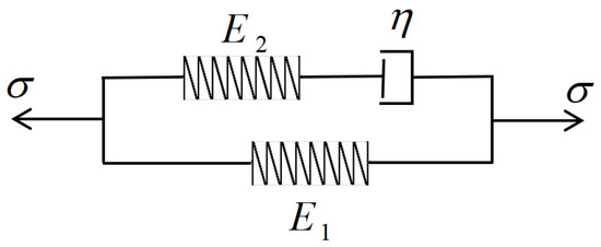
Figure 1.
The Zener model.
According to ref. [32], the relationship between virtual strain and virtual stress in the tensile direction can be expressed as
where the is an imaginary unit the is angular frequency; the viscoelastic parameters and can be expressed as
where the and are elastic modulus, the is the damping constant.
The pipeline material used in this study is PE100, and the dimensions of the tensile specimens strictly adhere to the Type B1 specifications outlined in the ISO 527-2:2012 standard (as shown in Figure 2). The testing environment was maintained at 20 °C. During the tests, the three specimens underwent constant-strain-rate tensile deformation at a strain rate of 10−1 s−1. Figure 2 presents the stress–strain relationship obtained from this series of tensile experiments.
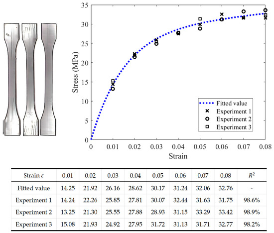
Figure 2.
The stress–strain relationship of the PE100 specimens with .
According to the Zener model, the following can be obtained
where the is stress; the is strain.
Because the experiment has a constant strain rate stretching (i.e., ), it can be expressed as
As shown in Appendix A, the following can be obtained
According to the experimental data, the material parameters of PE100 can be obtained as shown in Table 1.

Table 1.
The material parameters of PE100.
2.2. Dynamic Model of Irrigation Pipeline
As shown in Figure 3, the position function of irrigation pipelines is decomposed into the superposition of position functions of design configuration (the flexible straight beam) and micro-bending defect (the curve without change). The length of the design configuration is , and it is evenly divided into elements, each with a length of . The inner diameter is , the outer diameter is , and the relative velocity of fluid in the pipeline is . The rubber pipeline has initial micro bending defects , where the is the axis length coordinates of all pipelines.
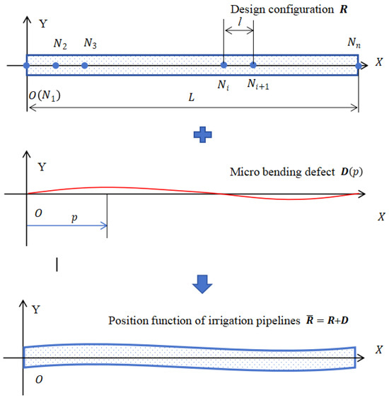
Figure 3.
Position function of irrigation pipelines.
As shown in Figure 4, the is a global coordinate system, and is the dimensionless elemental length coordinate of the elemental design configuration, .
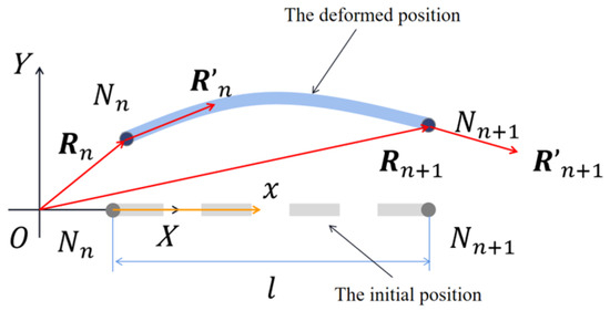
Figure 4.
Elemental design configuration.
The is the arbitrary point on the element, whose position vector in can be represented by . The can be expressed as
where the and are undetermined coefficients; the is time; the is an elemental shape function; the is a generalized coordinate column matrix of the irrigation pipeline; the is the Boolean matrix of the i-th element. They can be expressed as
where the are the position and unit tangent vector of node in ; the is identity matrix.
For the convenience of representation, the following calculations are defined as
The elemental position functions for micro-bending defects are expressed as . To balance the trade-off between geometric complexity and computational efficiency arising from small defects, a predefined constant correction function is introduced in the following two forms:
Form 1: Parabolic form (PF)
Form 2: Sine form (SF)
where the is the amplitude of the micro-bending defect.
The axis length coordinates of all pipelines can be expressed as , so that the elemental position functions of irrigation pipelines can be expressed as
And , , and .
Based on the equations of Lagrange written for a non-material volume [33], the nonlinear dynamic differential equation of an irrigation pipeline with stable stepped distribution flow velocity and fixed pipeline can be written as
where the and are kinetic energy of the pipeline and unit-volume fluid, respectively; the is relative velocity of the fluid, which can be expressed as = ; the and are the generalized elastic forces of the pipeline and elastic support, respectively. The kinetic energy of the pipeline and fluid can be written as and , respectively.
As shown in Figure 5, the displacement of the sprinkler is assumed to be a constant . Under ideal conditions, it can be concluded that
So the stable stepped distribution flow velocity can be expressed as
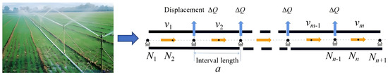
Figure 5.
Flow velocity distribution model.
The quantitative relationship between and can be compared by comparing the number of units and drainage holes.
The elemental kinetic energy of the pipeline and fluid can be expressed as
where the and is the outer and inner radius cross-sectional area of pipeline, respectively.
According to Equations (16) and (17), it can be obtained
According to the Euler-Bernoulli beam theory, the elemental elastic potential energy of the pipeline can be obtained as
where the and are the tensile stiffness and bending stifiness of the pipeline, respectively, both of which are functions of angular frequency ; the is initial curvature. The nonlinear axial Lagrange strain and the approximate high-order curvature of the element [34] can be expressed as
The high-order nonlinear generalized elastic force and generalized stiffness of pipeline can be expressed as
For an arbitrary point on the pipeline axis with , the displacement and rotation can be represented by and [28]. To approximate the clamped-supported boundary conditions of the pipeline, a penalty function is introduced to constrain the boundary points. This penalty function, formulated in an energy form, can be simplified as
where Pa.
The generalized force and generalized stiffness matrix corresponding to the boundary conditions can be written as
According to Equations (13) and (18), it can be expressed as
The equilibrium position of irrigation pipelines can be calculated by
The perturbation form of Equation (27) can be expressed as
If , Equation (29) can be expressed as
Then, the angular frequency can calculated by
2.3. Verification
2.3.1. Theoretical Verification
To validate the proposed model, a single-span circular cross-section beam was simulated using the material parameters listed in Table 1 (Section 2.1) and the additional parameters provided in Table 2. As demonstrated in Table 3, the first three natural vibration frequencies converge when the model is uniformly discretized into 15 or more elements. Consequently, a mesh resolution of 15 elements was adopted to ensure computational efficiency while maintaining accuracy.
Table 2.
The parameters of a single-span circular cross-section beam.
Table 3.
The first three orders of frequencies of a single-span circular cross-section beam (Until: rad/s).
These natural angular frequencies of this single-span straight pipeline with two clamped ends were calculated by the proposed model (PM) and finite element model (EFM), and the results are shown in Figure 6. The maximum relative error of the first three natural orders angular frequencies calculated by the two models is 3.21%.
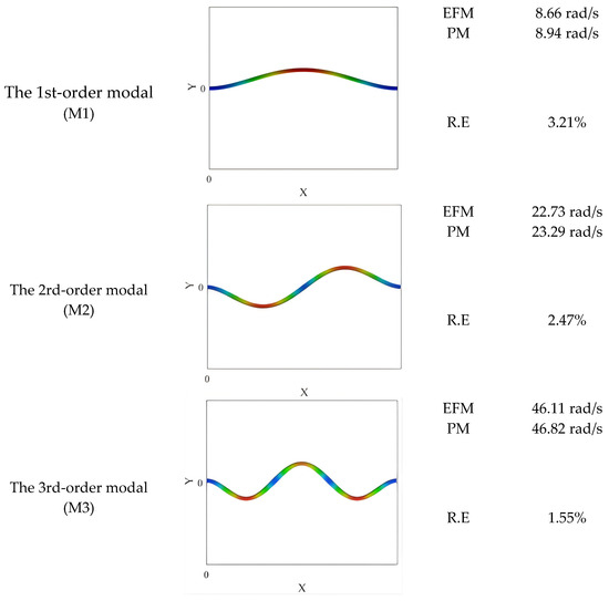
Figure 6.
The vibration characteristic of the single-span straight pipeline.
Figure 7 illustrates a non-uniform 7-span pipeline. The physical parameters of the pipeline are as follows: , , , , , , . Comparative analysis with ref. [33] shows that the calculation error of the proposed model with 15 elements is below 5%, indicating its capability to accurately predict the natural frequencies of a multi-span pipeline (as shown in Table 4).
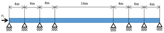
Figure 7.
The non-uniform 7-span pipeline.
Table 4.
The natural frequencies of the non-uniform 7-span pipeline.
2.3.2. Experimental Verification
The natural frequency of the irrigation pipeline was experimentally measured using a piezoelectric film sensor (LDTM-028K). As shown in Figure 8, the vibration detection system comprises three primary components: (1) the piezoelectric sensor, (2) a voltage amplifier, and (3) a data acquisition computer. Four sensors were deployed to capture the pipeline’s vibrational response under external excitation induced by an impulse hammer strike. Detailed pipeline parameters are provided in Table 5.
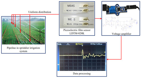
Figure 8.
The experimental testing of the irrigation pipeline.
Table 5.
The design parameters of the irrigation pipeline.
As shown in Figure 9, the simply supported points (the sprinkler bracket) are numbered and their position is determined through the survey. Based on the position of the simple pivot point, the irrigation pipelines can be seen as a micro-blanking pipeline (MBP) with parabolic defects. In order to verify the accuracy of the experimental results and the proposed micro-blanking pipeline model in this paper, the irrigation pipeline is also simplified into a multiple straight pipeline (MSP) model.
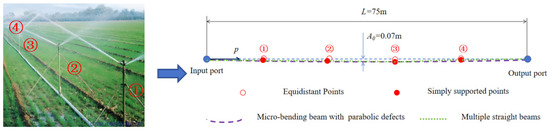
Figure 9.
The schematic diagram of irrigation pipeline.
As shown in Table 6, comparative analysis between experimental measurements and numerical simulations reveals that both the MBP (Micro-Bending Pipeline) and MSP (multiple straight pipeline) models demonstrate strong agreement with experimental data, exhibiting maximum relative errors below 8.43%. This close correlation confirms that the proposed micro-blanking pipeline model effectively predicts the vibration characteristics of irrigation pipelines, validating its accuracy for engineering applications.
Table 6.
The natural frequency of the irrigation pipeline (Until: rad/s).
As shown in Figure 10, when the flow velocity is zero, the imaginary component of the irrigation pipeline’s frequency exhibits non-zero values, with higher-order modes demonstrating progressively larger imaginary parts. At subcritical flow velocities below 6.27 m/s, the real frequency displays a gradual decreasing trend while maintaining positive values, accompanied by minimal variation in the imaginary component. This implies that the irrigation pipeline system preserves structural stability throughout this velocity range. However, when the flow velocity reaches or exceeds the critical threshold of 6.27 m/s, the first-order real frequency becomes 0 rad/s, while the imaginary component manifests asymmetric bifurcation characteristics. This bifurcation phenomenon signifies the system’s transition into distinct oscillation modes or resonance states. Notably, the irrigation pipeline’s small imaginary component rapidly decreases to negative values with increasing velocity, indicating that the system will undergo immediate divergent instability once the real component initiates from zero.
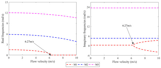
Figure 10.
The complex frequency of a rubber pipeline with different flow velocities.
The operational stability of piezoelectric film sensors is severely compromised when exposed to water-splashing environments generated by irrigation activities. Encapsulation with waterproof membranes leads to significant degradation in measurement accuracy. Moreover, the numerical simulations reveal that when the fluid velocity within irrigation pipelines exceeds the first-order critical speed threshold, the system rapidly enters a divergent instability state characterized by severe oscillations and noise, which are readily detectable by operators. Consequently, an integrated approach combining direct visual inspection and auditory monitoring has been adopted to assess pipeline stability.
Through controlled flow regulation and auditory monitoring of the irrigation pipeline, experimental observations indicate that when the inlet flow rate reaches 0.68 L/min, the pipeline system produces sharp popping sounds, and the irrigation sprinklers demonstrate noticeable shaking. With the inner radius , the critical flow velocity of this irrigation pipeline is approximately 6.26 m/s, which approaches the calculated critical flow velocity .
3. Stability Analysis and Improvement
As shown in Figure 11, the critical flow velocity of the pipeline with the sine form (SF) micro-bend defect is 7.41 m/s, which is 18.0% higher than that of the parabolic-form (PF) pipeline. In the proposed model of this study, the geometric configuration of the pipeline is described by superimposing a slight-curvature defect configuration onto the straight-tube baseline. All local coordinate systems are established based on the straight-tube reference, resulting in a concentrated mass distribution in the central region of the PF pipeline. This configuration consequently reduces the system’s natural frequency and critical flow velocity, compared to an SF pipeline with relatively uniform mass structure.
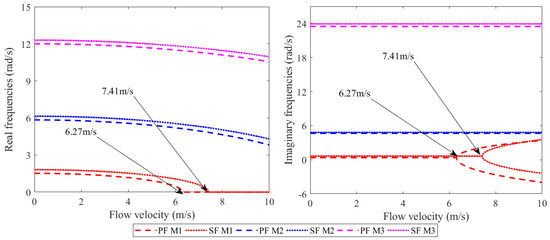
Figure 11.
The complex frequency of a rubber pipeline with different micro-bending defects.
As shown in Figure 12, with the increase in defect amplitude , the critical flow velocities of both pipeline types gradually rise, and the SF pipeline demonstrates a more pronounced enhancement. The heightened defect amplitude intensifies the pipeline curvature, thereby inducing localized stiffness reinforcement. The geometric characteristics of the PF pipeline predispose it to resonate with a specific mode of the first-order vibration pattern. When the defect amplitude increases, the first-order natural vibration frequency of the PF pipeline shifts toward higher frequencies at a slower rate compared to the SF pipeline.
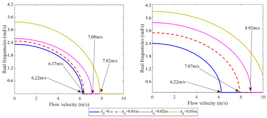
Figure 12.
The 1st order complex frequency of a rubber pipeline with different defect amplitudes.
The elemental position functions for micro-bending defects are set to
As Figure 13, the critical flow velocities initially exhibit an exponential increasing trend, as in
where the corresponds to the fundamental frequency of the design straight pipeline.
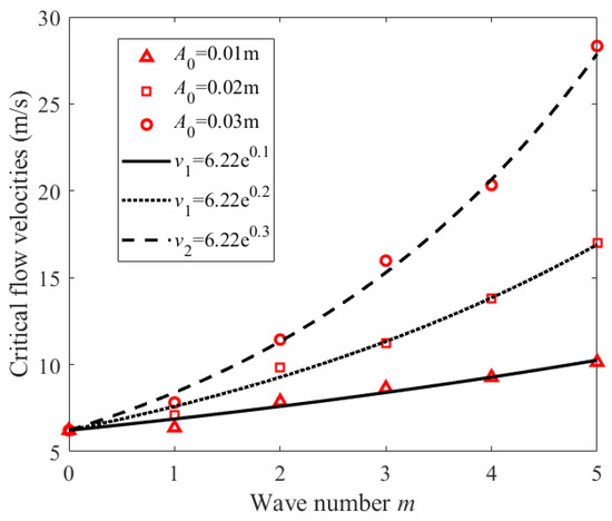
Figure 13.
The critical flow velocities of a rubber pipeline with different wave numbers.
If the pipeline exhibits irregular bending (e.g., localized abrupt changes or random fluctuations), the enhancing effect on the critical rotational speed will be reduced. Through manual adjustments, the sprinklers in the experimental pipeline were repositioned to create a non-standard sinusoidal-like curvature in the pipeline. Auditory and visual inspections by field technicians revealed significant noise and fluttering vibrations when the critical flow velocity reached approximately 7.14 m/s. This modification resulted in a 13.9% increase in pipeline flow rate.
4. Discussion
This study is based on the ANCF framework. By employing Lagrange equations for non-material volumes and introducing virtual elastic boundaries, a multi-span irrigation pipeline model with slight curvature defects is developed. To validate the model’s universality, it was degenerated into two classical structures: (1) simply supported uniform annular cross-section straight beams and (2) non-uniform 7-span fluid-conveying pipelines. Their natural frequencies were calculated and compared with finite element simulation results and theoretical solutions from other papers. The maximum relative error was below 4.83%, verifying the model’s validity.
Furthermore, field experiments on pipelines were conducted to measure natural frequencies and the first critical flow velocity. Compared with model predictions, the maximum error in natural frequencies was 8.43%, and the absolute error in the first critical flow velocity was only 0.01 m/s, further verifying the model’s practical reliability.
Through analysis and experimentation, it was found that as the initial waviness (wave number and amplitude) of irrigation pipelines increases within an appropriate range, the critical flow velocity of the pipeline gradually rises. This finding demonstrates consistency with the studies by Wang [36] and Ma [20]. Field experiments further demonstrated that irrigation pipelines with irregular sinusoidal defects exhibit a critical flow velocity of 7.14 m/s, which is 13.9% higher than that of pipelines with parabolic-like defects (6.26 m/s).
In the design of irrigation pipelines, considering pipeline length margin and potential initial curvature imperfections not only facilitates construction but also enables more economical and safer pipeline design. This is particularly critical in irrigation projects with limited pipe material options, tight flow design margins, and relatively low economic benefits.
Author Contributions
Conceptualization, B.F. and S.W.; methodology, B.F.; software, S.W. and J.C.; validation, B.F. and S.W.; formal analysis, S.X. and Y.C.; investigation, S.X.; resources, B.F. and S.W.; data curation, S.X.; writing—original draft preparation, B.F.; writing—review and editing, B.F.; visualization, S.W.; supervision, S.W.; project administration, J.C.; funding acquisition, S.W. All authors have read and agreed to the published version of the manuscript.
Funding
This research was funded by “Hainan Province Science and Technology Special Fund”, grant number ZDYF2025XDNY128.
Data Availability Statement
The datasets generated during and/or analyzed during the current study are available from the corresponding author on reasonable request.
Conflicts of Interest
The authors declare no conflicts of interest.
Abbreviations
The following abbreviations are used in this manuscript:
| ANCF | Absolute Nodal Coordinate Formulation |
Appendix A
For the Zener model, the total stress is the superposition of the spring and the Maxwell element, which can be expressed as
For the Maxwell element, the following can be obtained:
With , the following can be obtained
The homogeneous and specific solution of Equation (A3) can be written as
Due to the initial conditions with ,
By substituting Equation (A4) into Equation (A1), the following can be obtained
References
- Wang, H.; Zhao, J.; Zhang, L.; Yu, S. Application of Disturbance Observer-Based Fast Terminal Sliding Mode Control for Asynchronous Motors in Remote Electrical Conductivity Control of Fertigation Systems. Agriculture 2024, 14, 168. [Google Scholar] [CrossRef]
- Jia, W.; Wei, Z.; Tang, X.; Zhang, Y.; Shen, A. Intelligent control technology and system of on-demand irrigation based on multiobjective optimization. Agronomy 2023, 13, 1907. [Google Scholar] [CrossRef]
- Wang, T.; Wang, Z.; Zhang, J.; Ma, K. Application effect of different oxygenation methods with mulched drip irrigation system in Xinjiang. Agric. Water Manag. 2023, 275, 108024. [Google Scholar] [CrossRef]
- El-Sayed, T.A.; El-Mongy, H.H. Free vibration and stability analysis of a multi-span pipe conveying fluid using exact and variational iteration methods combined with transfer matrix method. Appl. Math. Model. 2019, 71, 173–193. [Google Scholar] [CrossRef]
- Amabili, M.; Garziera, R. Vibrations of circular cylindrical shells with nonuniform constraints, elastic bed and added mass; Part I: Empty and fluid-filled shells. J. Fluids Struct. 2000, 14, 669–690. [Google Scholar] [CrossRef]
- Pellicano, F.; Amabili, M. Dynamic instability and chaos of empty and fluid-filled circular cylindrical shells under periodic axial loads. J. Sound Vib. 2006, 293, 227–252. [Google Scholar] [CrossRef]
- Tsyss, V.G.; Sergaeva, M.Y. Simulating of the composite cylindrical shell of the pipe of the supply pipelines based on ANSYS package. Procedia Eng. 2016, 152, 332–338. [Google Scholar] [CrossRef][Green Version]
- Lee, U.; Jang, H.I. Go, Stability and dynamic analysis of oil pipelines by using spectral element method. J. Loss Prev. Process Ind. 2009, 22, 873–878. [Google Scholar] [CrossRef]
- Sınır, B.G.; Demir, D.D. The analysis of nonlinear vibrations of a pipe conveying an ideal fluid. Eur. J. Mech. B-Fluids 2015, 52, 38–44. [Google Scholar] [CrossRef]
- Li, Y.; Yang, Y. Vibration analysis of conveying fluid pipe via He’s variational iteration method. Appl. Math. Model. 2017, 43, 409–420. [Google Scholar] [CrossRef]
- Chernik, V.V. Analysis of dynamics and controllability of a system described by the equation of a pipeline with a moving fluid. IFAC-PapersOnLine 2018, 51, 156–161. [Google Scholar] [CrossRef]
- Khudayarov, B.A.; Komilova, K.M.; Turaev, F.Z. Numerical study of the effect of viscoelastic properties of the material and bases on vibration fatigue of pipelines conveying pulsating fluid flow. Eng. Fail. Anal. 2020, 115, 104635. [Google Scholar] [CrossRef]
- Nejadi, M.M.; Mohammadimehr, M.; Mehrabi, M. Free vibration and stability analysis of sandwich pipe by considering porosity and graphene platelet effects on conveying fluid flow. Alex. Eng. J. 2021, 60, 1945–1954. [Google Scholar] [CrossRef]
- Sutar, S.; Madabhushi, R.; Chellapilla, K.R.; Poosa, R.B. Determination of natural frequencies of fluid conveying pipes using Muller’s method. J. Inst. Eng. Ser. C 2019, 100, 449–454. [Google Scholar] [CrossRef]
- Sharififard, E.; Azizipour, M.; Ahadiyan, J.; Haghighi, A. Determinatin of creep function coefficients of viscoelastic pipes using a transient-guided machine learning model. AQUA-Water Infrastruct. Ecosyst. Soc. 2024, 73, 2132–2149. [Google Scholar] [CrossRef]
- Azizipour, M.; Sharififard, E.; Haghighi, A.; Ahadiyan, J. Optimization of creep function parameters of viscoelastic pipelines based on transient pressure signal. J. Hydraul. Struct. 2024, 10, 97–114. [Google Scholar] [CrossRef]
- Sinir, B.G. Bifurcation and chaos of slightly curved pipes. Math. Comput. Appl. 2010, 15, 490–502. [Google Scholar] [CrossRef]
- Farshidianfar, A.; Soltani, P. Nonlinear flow-induced vibration of a SWCNT with a geometrical imperfection. Comput. Mater. Sci. 2012, 53, 105–116. [Google Scholar] [CrossRef]
- Zhen, Y.; Gong, Y.; Tang, Y. Nonlinear vibration analysis of a supercritical fluid-conveying pipe made of functionally graded material with initial curvature. Compos. Struct. 2021, 268, 113980. [Google Scholar] [CrossRef]
- Ma, Y.; Wang, Z.; Fan, B.; Yong, X. Vibration characteristics of functionally graded fractional derivative viscoelastic fluid–conveying pipe with initial geometric defects. J. Eng. Mech. 2024, 150, 7419. [Google Scholar] [CrossRef]
- Chupakhin, A.; Mamontov, A.; Vasyutkin, S. Asymptotic representation of vorticity and dissipation energy in the flux problem for the navier–stokes equations in curved pipes. Axioms 2024, 13, 65. [Google Scholar] [CrossRef]
- Li, B.H.; Gao, H.S.; Zhai, H.B.; Liu, Y.S.; Yue, Z.F. Free vibration analysis of multi-span pipe conveying fluid with dynamic stiffness method. Nucl. Eng. Des. 2011, 241, 666–671. [Google Scholar] [CrossRef]
- Sollund, H.A.; Vedeld, K.; Hellesland, J.; Fyrileiv, O. Dynamic response of multi-span offshore pipelines. Mar. Struct. 2014, 39, 174–197. [Google Scholar] [CrossRef]
- Yang, Y.; Zhang, Y. Random vibration response of three-dimensional multi-span hydraulic pipeline system with multipoint base excitations. Thin-Walled Struct. 2014, 166, 108124. [Google Scholar] [CrossRef]
- Xu, W.; Jia, K.; Ma, Y.; Wang, Y.; Song, Z. Multispan classification methods and interaction mechanism of submarine pipelines undergoing vortex-induced vibration. Appl. Ocean Res. 2022, 120, 103027. [Google Scholar] [CrossRef]
- Wen, H.B.; Yang, Y.; Li, Y. Study on the stability of multi-span U-shaped pipe conveying fluid with complex constraints. Int. J. Press. Vessel. Pip. 2023, 203, 104911. [Google Scholar] [CrossRef]
- Oke, W.A.; Khulief, Y.A.; Owolabi, T.O.; Ikumapayi, O.M. Dynamic analysis of a multi-span pipe conveying fluid using wavelet based finite element method. Arab. J. Sci. Eng. 2024, 49, 14663–14682. [Google Scholar] [CrossRef]
- Fan, B.; Wang, Z.M. Vibration analysis of radial tire using the 3D rotating hyperelastic composite REF based on ANCF. Appl. Math. Model. 2024, 126, 206–231. [Google Scholar] [CrossRef]
- Liu, D.; Ai, S.; Sun, L.; Soares, C.G. ALE-ANCF modeling of the lowering process of a J-lay pipeline coupled with dynamic positioning. Ocean Eng. 2023, 269, 113552. [Google Scholar] [CrossRef]
- Yuan, J.R.; Ding, H. Three-dimensional dynamic model of the curved pipe based on the absolute nodal coordinate formulation. Mech. Syst. Signal Process. 2023, 194, 110275. [Google Scholar] [CrossRef]
- Xing, H.; He, Y.; Dai, H.; Wang, L. Design of simply support for fluid-conveying pipe with complex configurations based on absolute node coordinate formulation. Chin. J. Theor. Appl. Mech. 2024, 56, 482–493. (In Chinese) [Google Scholar] [CrossRef]
- Hosseini-Hashemi, S.; Abaei, A.R.; Ilkhani, M.R. Free vibrations of functionally graded viscoelastic cylindrical panel under various boundary conditions. Compos. Struct. 2015, 126, 1–15. [Google Scholar] [CrossRef]
- Irschik, H.; Holl, H.J. The equations of Lagrange written for a non-material volume. Acta Mech. 2002, 153, 231–248. [Google Scholar] [CrossRef]
- Fan, B.; Wang, Z.M.; Wang, Q.B. Nonlinear forced transient response of rotating ring on the elastic foundation by using adaptive ANCF curved beam element. Appl. Math. Model. 2022, 108, 748–769. [Google Scholar] [CrossRef]
- Wu, J.S.; Shih, P.Y. The dynamic analysis of a multispan fluid-conveying pipe subjected to external load. J. Sound Vib. 2001, 239, 201–215. [Google Scholar] [CrossRef]
- Wang, Z.M.; Liu, Y.Z. Transverse vibration of pipe conveying fluid made of functionally graded materials using a symplectic method. Nucl. Eng. Des. 2016, 298, 149–159. [Google Scholar] [CrossRef]
Disclaimer/Publisher’s Note: The statements, opinions and data contained in all publications are solely those of the individual author(s) and contributor(s) and not of MDPI and/or the editor(s). MDPI and/or the editor(s) disclaim responsibility for any injury to people or property resulting from any ideas, methods, instructions or products referred to in the content. |
© 2025 by the authors. Licensee MDPI, Basel, Switzerland. This article is an open access article distributed under the terms and conditions of the Creative Commons Attribution (CC BY) license (https://creativecommons.org/licenses/by/4.0/).