Spatial–Temporal Variability of Soybean Yield Using Separable Covariance Structure

Abstract

(1) Understanding and characterizing the spatial and temporal variability of agricultural data is a key aspect of precision agriculture, particularly in soil management. Modeling the spatiotemporal dependency structure through geostatistical methods is essential for accurately estimating the parameters that define this structure and for performing Kriging-based interpolation. This study aimed to analyze the spatiotemporal variability of the soybean yield over ten crop years (2012–2013 to 2021–2022) in an agricultural area located in Cascavel, Paraná, Brazil. (2) Spatial analyses were conducted using two approaches: the Gaussian linear spatial model with independent multiple repetitions and the spatiotemporal model with a separable covariance structure. (3) The results showed that the maps generated using the Gaussian linear spatial model with multiple independent repetitions exhibited similar patterns to the individual soybean yield maps for each crop year. However, when comparing the kriged soybean yield maps based on independent multiple repetitions with those derived from the spatiotemporal model with a separable covariance structure, the accuracy indices indicated that the maps were dissimilar. (4) This suggests that incorporating the spatiotemporal structure provides additional information, making it a more comprehensive approach for analyzing soybean yield variability. The best model was chosen through cross-validation and a trace. Thus, incorporating a spatiotemporal model with a separable covariance structure increases the accuracy and interpretability of soybean yield analyses, making it a more effective tool for decision-making in precision agriculture.

1. Introduction

Nowadays, it is extremely important to search for optimal solutions to the most varied problems in the agricultural sector because the complete immersion in concepts such as performance, efficiency, and costs makes the agricultural sector seek greater sustainability in competitive markets. In this way, researchers and farmers are acquiring the system of sustainable agriculture, called precision agriculture (PA) [1]. PA enables localized crop management, with the application of the adequate amount of input to each site, thus reducing environmental costs and risks [2].

Furthermore, soils are not uniformly distributed across the Earth’s surface, exhibiting varying degrees of homogeneity depending on the region [3]. Even soils considered homogeneous still display spatial and temporal variability in their chemical, physical, and biological properties. This variability in crop production can be influenced by multiple factors, including climate, genetics, soil characteristics, topography, management practices, pests, diseases, and the dynamic interaction between all the above-mentioned factors [4].

Thus, knowing and defining the spatial and temporal variability of data and agricultural yields becomes an important factor for the realization of soil management [1]. The study of this spatial and temporal variability of georeferenced variables can be carried out by geostatistical techniques, which determine the degree of spatial dependence between the sample elements in the region and the degree of temporal dependence in the crop years under study, describing the spatiotemporal dependency structure of the georeferenced variable throughout the area, thus elaborating the thematic maps through Kriging interpolation. Spatiotemporal, geostatistical modeling is an empirical approach that involves specifying a model and estimating its parameters based on observed data. These models are particularly useful when data are repeatedly collected at the same sampling locations over both space and time [5,6,7,8,9].

The application of spatiotemporal models in agriculture is increasingly being used, and several studies in the literature have examined the spatiotemporal relationships of soil’s physical and chemical attributes. For instance, ref. [3] analyzed the spatiotemporal variability of soil’s chemical attributes between the 2013–2014 and 2017–2018 harvests. Also, ref. [10] investigated the spatiotemporal evolution of the micronutrients available in the soil, while ref. [11] explored the effects of soil carbon and nitrogen on temporal and spatial variations in the soil. Furthermore, ref. [12] studied a Gaussian spatiotemporal model with a separable covariance structure developing an analysis of local influence diagnoses.

Therefore, analyzing the spatial and temporal variability of soybean productivity is essential for soil management, as well as for forecasting the coming years. The greatest contribution of this work is the use of the function ${\mathit{\Sigma }}_{TS}={\mathit{\Sigma }}_T\otimes {\mathit{\Sigma }}_S={\mathit{R}}_T{(\phi }_4)\otimes \left({\phi }_1{\mathit{I}}_{\mathit{n}}+{\phi }_2{\mathit{R}}_s\left(\tau \right)\right)$, while considering the parameter ${\tau =\mathsf{\phi }}_3$ as fixed a priori. Furthermore, to avoid identifiability problems, reparameterization was used for the spatial covariance function ${\mathit{\Sigma }}_S$ of the Matérn family. While ref. [9] considered each crop year as a realization of the process and the Gaussian spatial model with multiple independent repetitions, [12] used a Gaussian space-time model with a separable covariance structure considering identifiability and the parameter ${\tau =\mathsf{\phi }}_3$ as fixed; however, they did not consider reparameterization.

The objective of this study was to analyze the spatiotemporal variability of the soybean yield (t ha⁻¹) over ten crop years (2012–2013 to 2021–2022) in a commercial grain production area. By applying geostatistical methods, the aim was to evaluate the spatial and temporal dependencies in the yield distribution, providing insights into the patterns and trends that influence productivity over time.

The work is organized as follows. Section 2 describes the data and the methodologies employed to analyze the spatiotemporal variability of the soybean yield, including the geostatistical methods and model estimation techniques used to handle the multi-year crop data. Section 3 presents the results of the study, focusing on the spatiotemporal variability of the soybean yield. The discussion and conclusions are in Section 4 and Section 5, respectively.

2. Materials and Methods

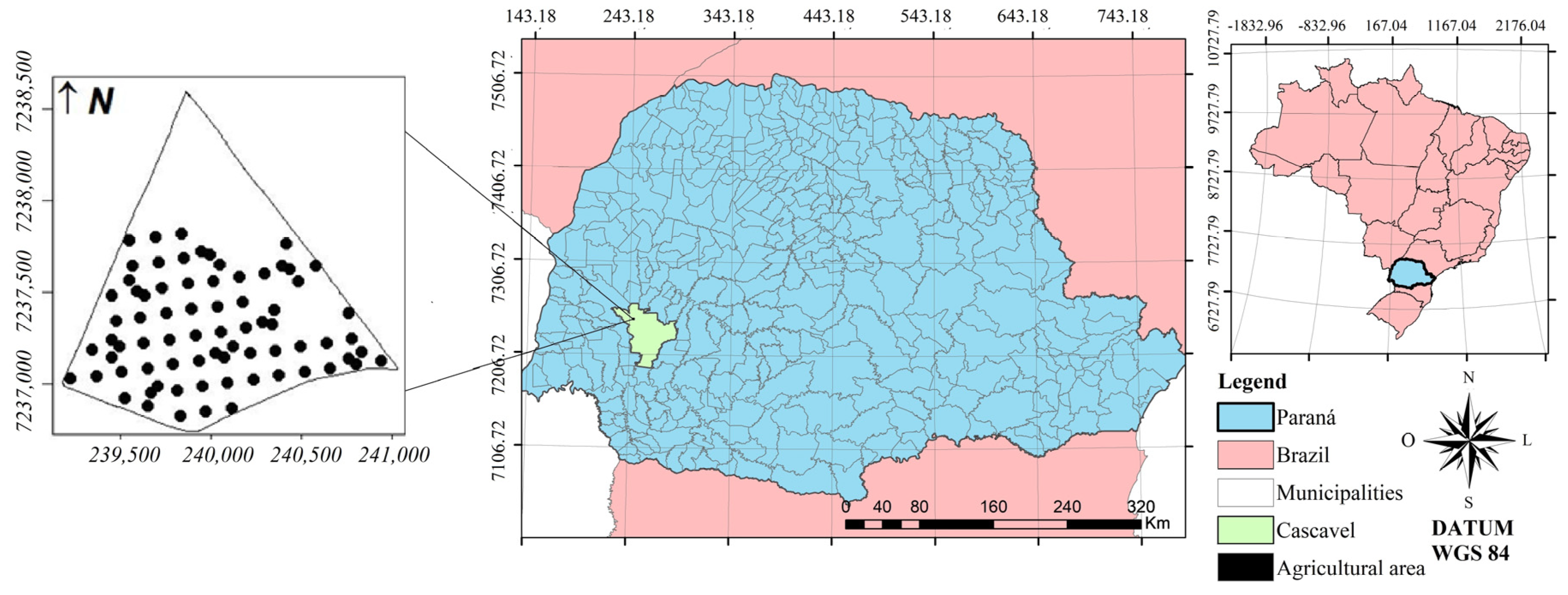
2.1. Description of Agricultural Area

The ten-year crop dataset used in this research belongs to the database of projects developed by researchers from the research group of the Space Statistics Laboratory (LEE) and the Applied Statistics Laboratory (LEA) of the West Parana State University—UNIOESTE, Campus Cascavel. Data collection was carried out in a commercial grain production area of 167.35 ha, located in the city of Cascavel-Paraná-Brazil, approximately 24.95° south, 53.37° west, and at a 650 m average altitude. The soil is classified as a typical Dystroferric Red Latosol, with a clayey texture [13]. The climate of the region is classified as mesothermic and superhumid temperate, climate type Cfa (Koeppen), and the average annual temperature is 21 °C [14].

The sample configuration of the area under study was a lattice with close pairs [15,16], with $n$ = 74 sampling points (Figure 1). This sample configuration consists of a regular grid with a minimum distance of 141 m between the points, and in some randomly chosen places, the sampling points were arranged in smaller distances (75 and 50 m between the pairs of points). The samples were located and georeferenced by a GPS receiver in a Datum WGS84 coordinate reference system, with UTM (Universal Transverse Mercator) projection.

Figure 1. Sampling points of the study area.

Soil sampling was performed at each demarcated point of the agricultural area (Figure 1). In accordance with the recommendations found in the literature, four soil subsamples were collected at these points from depths of 0.0 to 0.2 m deep [17], mixed, and placed in plastic bags; the samples were approximately 500 g in weight, thus composing the representative sample of the plot. The chemical analyses were performed using the Walkley–Black method [18].

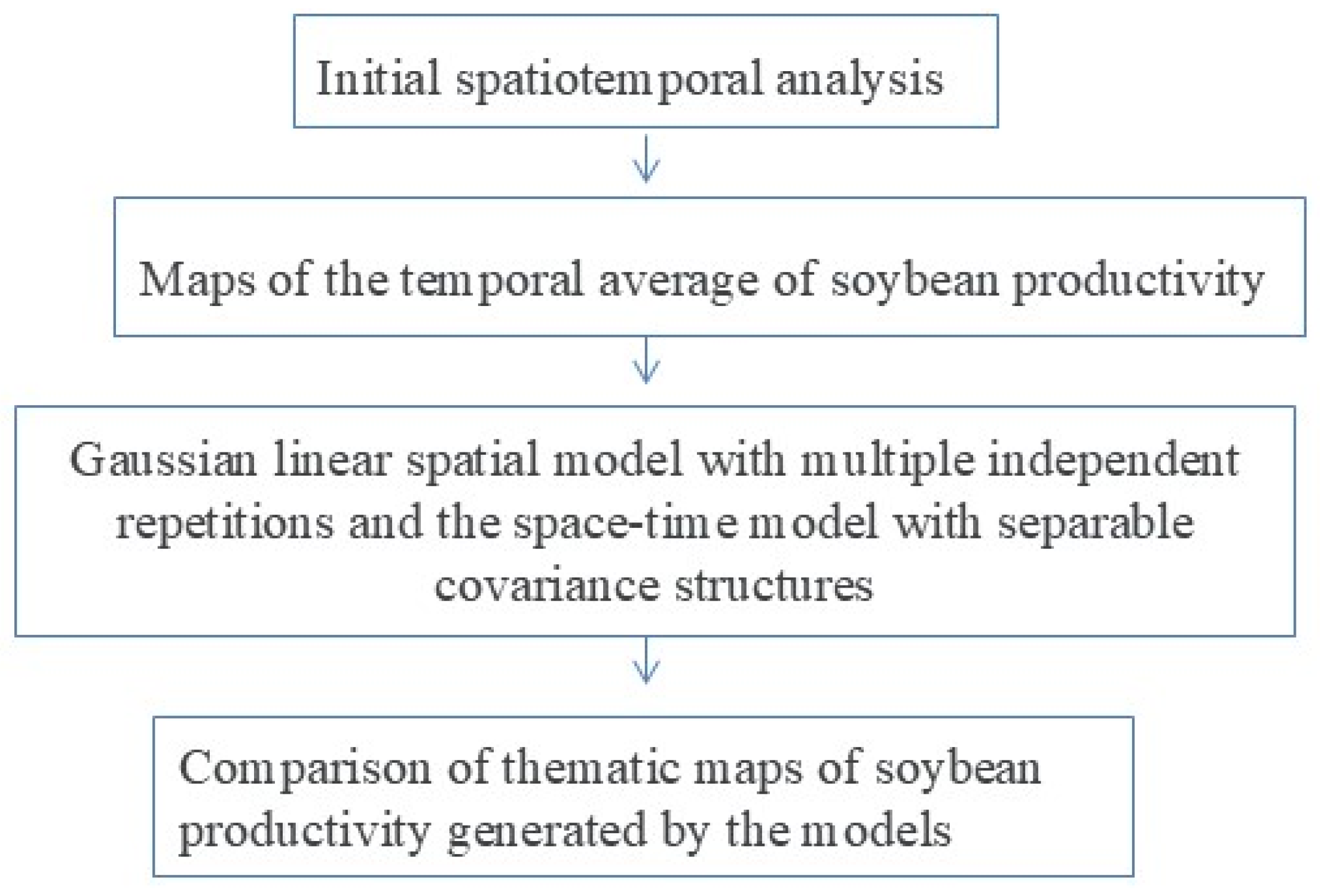
2.2. Methodology: Spatiotemporal Analysis

Initially, the spatiotemporal exploratory analysis of the soybean yield was carried out, considering the ten-year crop: 2012–2013, 2013–2014, 2014–2015, 2015–2016, 2016–2017, 2018–2019, 2019–2020, 2020–2021, 2021–2022, and 2022–2023. Subsequently, maps were created with the temporal averages of the soybean yield considering all the spatial locations, as well as the spatial averages of the soybean yield considering all the crop years. Finally, a Gaussian linear spatial model with multiple independent repetitions and a spatiotemporal model with a separable covariance structure were carried out (Figure 2).

Figure 2. Spatiotemporal methodology.

2.3. Gaussian Linear Spatial Model with Multiple Independent Repetitions

Let $\mathit{Y}=\mathit{Y}\left(\mathit{s}\right)=vec\left({\mathit{Y}}_1\right(\mathit{s}),...,{\mathit{Y}}_{\mathit{T}}(\mathit{s}\left)\right)$ be a random vector $nT\times 1$ of $T$ stochastic processes, independent of each $n$ element, belonging to the family of Gaussian, and with dependent distributions in the ${\mathit{s}}_j\in \mathit{S}\subset {\mathit{R}}^2$ positions $j=1,...,n$ for $\mathit{s}={({\mathit{s}}_1,...,{\mathit{s}}_n)}^T$. In this study, ${\mathit{Y}}_{\mathit{i}}$ represents the soybean yield in each crop year $i$, and $i=1,...,10\left(T=10\right)$ for the samples collected in 74 sampling points $(n=74)$. The i-th stochastic process ${\mathit{Y}}_{\mathit{i}}\left(\mathit{s}\right)$ is an $n\times 1$ vector, $i=1,...,T$, and it can be expressed by the model given in Equation (1).

$${\mathit{Y}}_i\left(\mathit{s}\right)={\mathit{\mu }}_i\left(\mathit{s}\right)+{\mathit{ϵ}}_{\mathit{i}}\left(\mathit{s}\right),$$

(1)

where ${\mathit{\mu }}_{\mathit{i}}\left(\mathit{s}\right)$ is the deterministic term; and ${\mathit{ϵ}}_{\mathit{i}}\left(\mathit{s}\right)$ is the stochastic error vector $n\times 1$ of the stationary isotropic process with the zero mean vector $E\left[{\mathit{ϵ}}_{\mathit{i}}\left(\mathit{s}\right)\right]=0$ and the spatial covariance matrix ${\mathit{\Sigma }}_S={\mathit{\Sigma }}_{\mathit{i}}=\left[C\left(s_u,s_v\right)\right]$ $n\times n$, this being the covariance matrix ${\mathit{Y}}_i$ for the $i$-th repetition $i=1,...,T$. The ${\mathit{\Sigma }}_{\mathit{i}}$ matrix is non-singular, symmetrical, and positively defined.

The spatial covariance matrix is considered to be ${\mathit{\Sigma }}_S$, the same for each repetition, and has a structure that depends on the $\mathit{\phi }={({\phi }_1,\dots ,{\phi }_q)}^T$ parameters, as given in Equation (2) [19,20].

$${\mathit{\Sigma }}_S={\phi }_1{\mathit{I}}_n+{\phi }_2{\mathit{R}}_S\left({\phi }_3\right),$$

(2)

where ${\phi }_1\ge 0$ is the nugget effect; ${\mathit{I}}_{\mathit{n}}$ is the identity matrix $n\times n$; ${\phi }_2\ge 0$ is the contribution; ${\phi }_3\ge 0$ is the function of the ($a$) range of the model; that is, $a=g\left({\phi }_3\right)$. The ${\mathit{R}}_S\left({\phi }_3\right)$ matrix is in the function of ${\phi }_3$, with ${\mathit{R}}_S={\mathit{R}}_S\left({\phi }_3\right)=\left[\left(r_{uj}\right)\right]$ being an $n\times n$ symmetric matrix, in which $r_{uj}$ depends only on the Euclidean distance between ${\mathit{s}}_u$ and ${\mathit{s}}_j$($h_{uj}=‖{\mathit{s}}_u-{\mathit{s}}_j‖$), with the diagonal elements $r_{uj}=1$, for $u=j$; $r_{uj}={\phi }_2^{-1}C({\mathit{s}}_{\mathit{u}},{\mathit{s}}_{\mathit{j}})$ for ${\phi }_2\ne 0$ and $u\ne j$; and $r_{uj}=0$ for ${\phi }_2=0$ and $u\ne j(u,j=1,\dots ,n)$ [20,21,22].

The logarithm of the likelihood function for $T$ independent repetitions is defined according to Equation (3).

$$\mathcal{L}\left(\mathit{\theta }\right)=\sum _{i=1}^T(-{\displaystyle \frac{n}{2}}\mathit{log}\left(2\pi \right)-{\displaystyle \frac{1}{2}}\mathit{log}\left|\mathit{\Sigma }\right|)-{\displaystyle \frac{1}{2}}\sum _{i=1}^T{{\left({\mathit{Y}}_i-\mu 1\right)}^T\mathit{\Sigma }}^{-1}\left({\mathit{Y}}_i-\mu 1\right).$$

(3)

Further information and details of the Gaussian linear spatial model with multiple independent repetitions can be obtained from [9].

2.4. Linear Spatiotemporal Model

Here, $\left\{\mathit{Y}\right(\mathit{s},t):\mathit{s}\in \mathit{S}\subset {\mathbb{R}}^d,t\in \mathfrak{I}\subset \mathbb{R}\}$ defines a spatiotemporal process, where $\mathit{S}$ is the spatial domain of interest, and $\mathfrak{I}$ is the temporal domain of interest. The Gaussian stochastic $\mathit{Y}(\mathit{s},t)$ process is defined in several fixed monitoring locations, ${\mathit{s}}_1,\dots ,{\mathit{s}}_n\in \mathit{S}\subset {\mathbb{R}}^d$, with $d\ge 2$, and in time $t_1,\dots ,t_T\in {\rm T}\subset \mathbb{R}$. It can be expressed as a regression model given by Equation (4).

$$\mathit{Y}\left({\mathit{s}}_j,t\right)=\mathit{\mu }\left({\mathit{s}}_j,t\right)+\mathit{ϵ}\left({\mathit{s}}_{\mathit{j}},t\right),$$

(4)

where $j=1,\dots ,n$ $(n=74)$ and $t=1,\dots ,{\rm T}$ $(T=10)$; $\mathit{\mu }\left({\mathit{s}}_j,t\right)$ is the deterministic term; and $\mathit{ϵ}\left({\mathit{s}}_j,t\right)$ is the stochastic error vector with a zero mean vector, $E\left[\mathit{ϵ}\left({\mathit{s}}_j,t\right)\right]=0$, and a spatiotemporal covariance structure ${\mathit{\Sigma }}_{TS}$.

The spatiotemporal covariance function ${\mathit{\Sigma }}_{TS}$ for the process $\mathit{Y}\left(\mathit{s},t\right)$ is denoted by ${\mathit{\Sigma }}_{TS}=C\left({\mathit{s}}_1,{\mathit{s}}_2;t_1,t_2\right)=C\left[ϵ\left({\mathit{s}}_1,t_1\right),ϵ\left({\mathit{s}}_2,t_2\right)\right].$

A random spatiotemporal field presents the stationary covariance in space if $Cov\left(\mathit{Y}\right({\mathit{s}}_1,t_1,{\mathit{s}}_2,t_2\left)\right)$ depends only on the vector $\mathit{h}={\mathit{s}}_1-{\mathit{s}}_2,$ while it presents temporal stationarity $Cov\left(\mathit{Y}\right({\mathit{s}}_1,t_1,{\mathit{s}}_2,t_2\left)\right)$ if it depends only on the $u=t_1-t_2$ vector. Therefore, if the random spatiotemporal field has stationary covariance in space and time, the spatiotemporal covariance is given by Equation (5) [23,24,25].

$$Cov\left(Y\left({\mathit{s}}_1,t_1\right),Y\left({\mathit{s}}_2,t_2\right)\right)=Cov\left({\mathit{s}}_1-{\mathit{s}}_2;t_1-t_2\right)=C\left(\mathit{h},u\right).$$

(5)

The process is said to be isotropic if $C\left(\mathit{h},u\right)=C(‖\mathit{h}‖;\left|u\right|)$; that is, the covariance function depends on the separation vectors only by their $‖\mathit{h}‖$ lengths $\left|u\right|$ and not by the direction [12].

2.5. Spatiotemporal Covariance Models with Separable Covariance Structure

The separable spatiotemporal covariance functions can be defined based on the properties of additivity and multiplicativity [23]. Thus, it can be decomposed between a purely spatial covariance function and a purely temporal one; for the additive case, this can be written as Equation (6) [23].

$$Cov\left(\mathit{Y}\left({\mathit{s}}_1,t_1\right),\mathit{Y}\left({\mathit{s}}_2,t_2\right)\right)=Cov\left(\mathit{Y}\left({\mathit{s}}_1,{\mathit{s}}_2\right)\right)+Cov\left(\mathit{Y}\left(t_1,t_2\right)\right).$$

(6)

And for the multiplicative case, this can be written as Equation (7) [23].

$$Cov\left(\mathit{Y}\left({\mathit{s}}_1,t_1\right),\mathit{Y}\left({\mathit{s}}_2,t_2\right)\right)=Cov\left(\mathit{Y}\left({\mathit{s}}_1,{\mathit{s}}_2\right)\right)·Cov\left(\mathit{Y}\left(t_1,t_2\right)\right),$$

(7)

and in both cases, ${\mathit{s}}_1,t_1$ and ${\mathit{s}}_2,t_2\in {\mathbb{R}}^d\times \mathbb{R}$. However, all the separable models also present symmetry [23].

For spatiotemporal modeling with the separable covariance ${\mathit{\Sigma }}_{TS}={\mathit{\Sigma }}_T\otimes {\mathit{\Sigma }}_S$, the Matérn family [26] is a particularly attractive covariance function, where the elements of the correlation matrix, $\mathit{R}=\left[\right(r_{ij}\left)\right],$ are given by Equation (8).

$$r_{ij}={\displaystyle \frac{1}{2^{\kappa -1}\Gamma \left(k\right)}}{\left({\displaystyle \frac{{\delta }_{ij}}{\tau }}\right)}^{\kappa }{K}_{\kappa }\left({\displaystyle \frac{{\delta }_{ij}}{\tau }}\right),$$

(8)

where $\tau >0$ and $\kappa >0$ are parameters; ${\delta }_{ij}$> 0 can be the euclidean distance between ${\mathit{s}}_i$ points; and ${\mathit{s}}_j$ $i,j=1,...,n$, considering the spatial ${\mathit{\Sigma }}_{\mathit{S}},$ considering the structure or distance in time $|t_i-t_j|,i,j=1,...,T$, and considering the temporal structure ${\mathit{\Sigma }}_{\mathit{T}}$; $K_k$ is the third-order-modified Bessel function, $K_k\left(u\right)={\displaystyle \frac{1}{2}}{\int }_0^{\mathrm{\infty }}{x}^{k-1}{e}^{{\displaystyle \frac{1}{2}}u\left(x+{\displaystyle \frac{1}{x}}\right)}dx$, and this function is valid for $\tau$ and $\kappa$ greater than zero. In this family, the $\kappa$ parameter, called smoothing, consists of a parameter that determines the analytical smoothing of the underlying process $\mathit{Y}(\mathit{s},t)$ [27].

In this study, we chose to work with spatiotemporal modeling with separable covariance, of the Matérn family, Equation (8), due to its applicability and the variation of the model’s k parameter, and because the data present a multivariate normal distribution. The choice of spatiotemporal separability was used to overcome the computational complexity of non-separable models [25]. However, it was not feasible to apply a formal separability test, such as those proposed by [28], due to the limited temporal extent of our dataset (10 crop years). These tests require a minimum of 29 years of temporal observations. Consequently, we adopted the assumption of covariance separability in this study. For these reasons, we assume the separability of covariance at work.

2.6. Estimation Methods

2.6.1. Identifiability of the Model

The identifiability of the statistical model is an important step in a spatiotemporal study because if the model is not identifiable, there are no consistent estimators for the parameter vector. This identifiability allows us to guarantee the uniqueness of the distribution according to the parameters [29].

To remove the problems of identifiability in spatial dependence, it is assumed that the ${\tau =\phi }_3$ range parameter is fixed a priori in Equation (8) [29,30,31,32]. Thus, a reparameterization was used for the function of spatial covariance ${\mathit{\Sigma }}_s$ of the Matérn family, according to Equation (9) [33].

$$C\left({\delta }_{ij}\right)={\phi }_1{\xi }_{ij}+{\displaystyle \frac{{\phi }_2^{*}}{2^{\kappa -1}\Gamma \left(k\right)}}{\left({\delta }_{ij}{\phi }_3\right)}^{\kappa }{K}_{\kappa }\left({\displaystyle \frac{{\delta }_{ij}}{{\phi }_3}}\right), {\delta }_{ij}\ge 0$$

(9)

in which ${\phi }_1\ge 0$ is the nugget effect; ${\phi }_3\ge 0$ is the function of the ($a$) range of the model, that is, $a=g\left({\phi }_3\right)$; and ${\xi }_{ij}$ is the Kronecker delta, $i,j=1,\dots ,n$, with ${\phi }_2^{*}={\displaystyle \frac{{\phi }_2}{{\left({\phi }_3\right)}^{2\kappa }}}$. If ${\phi }_3$ is fixed a priori, the covariance matrix for spatial dependence ${\mathit{\Sigma }}_{\mathit{S}}$ has a linear structure [20]. Thus, the covariance structure of the separable ${\mathit{\Sigma }}_{\mathit{T}\mathit{S}}={\mathit{\Sigma }}_T\otimes {\mathit{\Sigma }}_S$ matrix has, as elements, the matrices given by Equation (10).

$${\mathit{\Sigma }}_{\mathit{T}}={\mathit{R}}_T{(\phi }_4), \mathrm{a}\mathrm{n}\mathrm{d} {\mathit{\Sigma }}_{\mathit{S}}={\phi }_1{\mathit{I}}_{\mathit{n}}+{\phi }_2^{*}{\mathit{R}}_{\mathit{S}}\left({\phi }_3\right),$$

(10)

where ${\mathit{\Sigma }}_{\mathit{S}}$ defines the spatial dependency structure, ${\mathit{I}}_n$ is the identity $n\times n$ matrix, ${\phi }_1$ is the nugget effect, ${\phi }_2^{*}$ is a function of the contribution parameter ${\phi }_2$, ${\mathit{R}}_{\mathit{S}}({\phi }_3$) is a matrix that is ${\phi }_3$ fixed, and ${\mathit{\Sigma }}_{\mathit{T}}$ defines the temporal dependency structure, with ${\mathit{R}}_{\mathit{T}}{(\phi }_4)$ being the matrix defined in Equation (8) as a function of ${\phi }_4$.

The particular case of Equation (10) allows us to consider the structure ${\mathit{\Sigma }}_{\mathit{T}}$ that defines the temporal dependency structure as ${\mathit{\Sigma }}_{\mathit{T}}={\mathit{I}}_T$ (${\mathit{I}}_T$ being the temporal identity matrix) and use the development of Section 2.3, considering the analysis of the Gaussian linear spatial model with multiple independent repetitions.

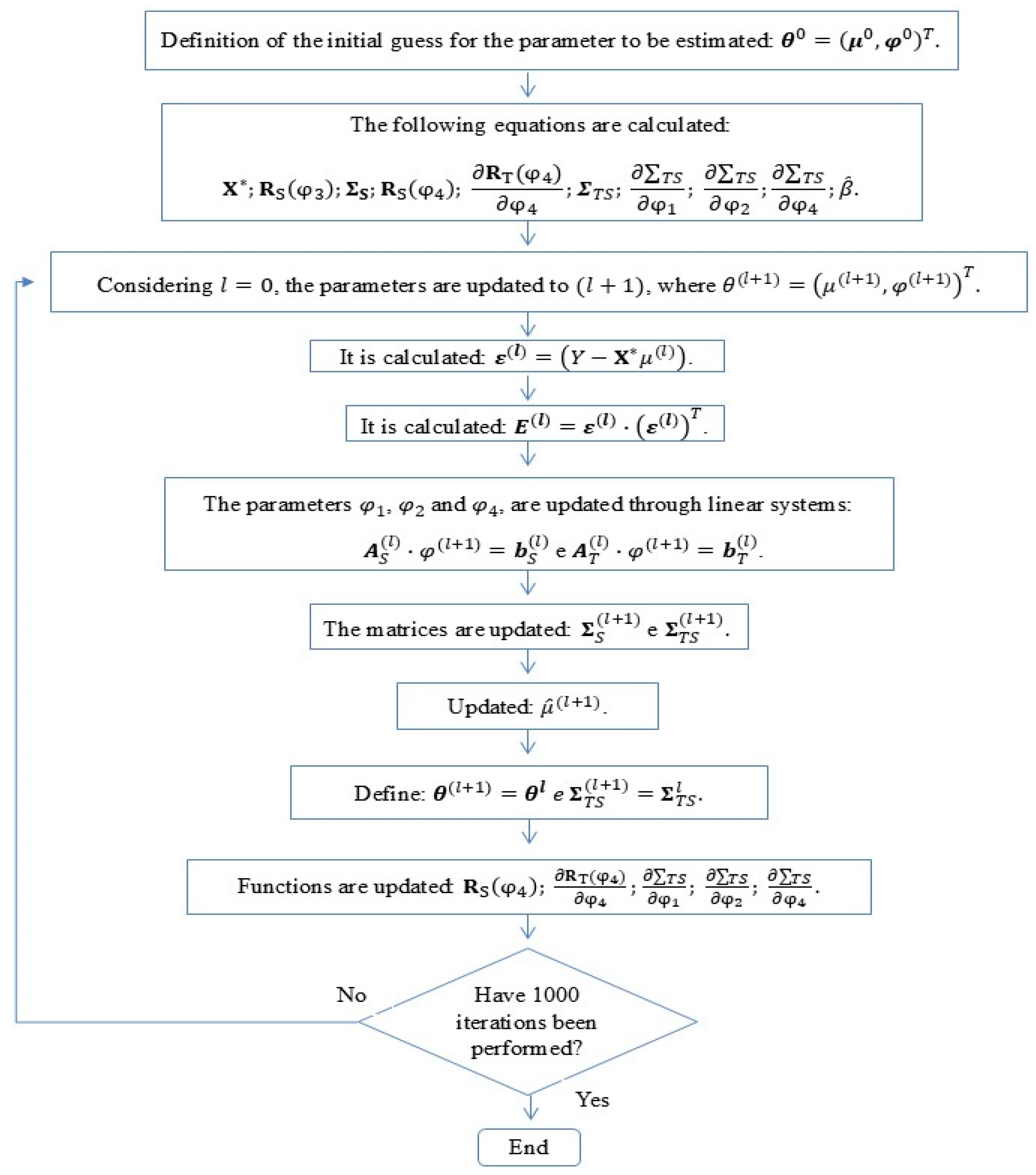
2.6.2. The Estimation of Parameters by Maximum Likelihood for the Separable Model

In the spatiotemporal model defined in Equation (4), considering $\mathit{\mu }\left({\mathit{s}}_i,t\right)=\left(1_{\mathit{t}}⨂1_{\mathit{n}}\right)\mu ,$ under the assumption of the normality of errors and considering a separate covariance matrix ${\mathit{\Sigma }}_{\mathit{T}\mathit{S}}={\mathit{\Sigma }}_{\mathit{T}}\otimes {\mathit{\Sigma }}_{\mathit{S}}$, the vector $\mathit{Y}=\mathit{Y}\left(\mathit{s},t\right)$ has a varied normal distribution $nT$, as described in Equation (11).

$$\mathit{Y}~N_{nT}\left({\mathit{X}}^{*}\mu ,{\mathit{\Sigma }}_{TS}\right),$$

(11)

where ${\mathit{X}}^{*}=(1_{\mathit{t}}⨂1_{\mathit{n}})$ and ${\mathit{\Sigma }}_{\mathit{T}\mathit{S}}={\mathit{\Sigma }}_T\otimes {\mathit{\Sigma }}_{\mathit{S}}$, with ${\mathit{\Sigma }}_{\mathit{T}}$ and ${\mathit{\Sigma }}_{\mathit{S}}$ being the matrices of temporal and spatial covariance, respectively. The logarithm of the likelihood function of $\mathit{Y}$ is given by Equation (12).

$$\mathcal{L}\left(\mathit{\theta }\right)=-{\displaystyle \frac{nT}{2}}log\left(2\pi \right)-{\displaystyle \frac{1}{2}}log\left|{\mathit{\Sigma }}_{\mathit{{\rm T}}\mathit{S}}\right|-{\displaystyle \frac{1}{2}}{\left(\mathit{Y}-{\mathit{X}}^{*}\mu \right)}^T{\mathit{\Sigma }}_{\mathit{{\rm T}}\mathit{S}}^{-1}\left(\mathit{Y}-{\mathit{X}}^{*}\mu \right),$$

(12)

where $n$ is the sample size; $T$ is the number of crop years; ${\mathit{\Sigma }}_{\mathit{T}\mathit{S}}={\mathit{\Sigma }}_T\otimes {\mathit{\Sigma }}_{\mathit{S}};\mathbf{Y}=\mathit{Y}\left(\mathit{s},t\right);{\mathit{X}}^{*}=\left(1_{\mathit{t}}⨂1_{\mathit{n}}\right);\mathit{\theta }={(\mu ,{\mathit{\phi }}^{\mathit{T}})}^T;$ and $\mathit{\phi }={({\phi }_1,{\phi }_2,{\phi }_4)}^T$ is a vector that contains unknown parameters of the spatiotemporal covariance matrix.

The function scores are obtained by calculating $U\left(\mu \right)$ and $U\left(\mathit{\phi }\right)$ as follows.

$$U\left(\mathit{\theta }\right)={\left({U\left(\mu \right)}^{\mathit{T}},{U\left(\mathit{\phi }\right)}^{\mathit{T}}\right)}^{\mathit{T}},$$

where

$$U\left(\mu \right)={\displaystyle \frac{\partial \mathcal{L}\left(\mathit{\theta }\right)}{\partial \mathit{\mu }}}={\mathit{X}}^{*\mathit{T}}{\mathit{\Sigma }}_{\mathit{T}\mathit{S}}^{-1}\mathsf{\epsilon },U\left({\phi }_j\right)={\displaystyle \frac{\partial \mathcal{L}\left(\mathit{\theta }\right)}{\partial {\phi }_j}}=-{\displaystyle \frac{1}{2}}\left\{tr\left({\mathit{\Sigma }}_{\mathit{T}\mathit{S}}^{-1}{\displaystyle \frac{{\partial \Sigma }_{sT}}{\partial {\phi }_j}}\right)+{\displaystyle \frac{1}{2}}{\mathit{\epsilon }}^{\mathit{T}}\left({\mathit{\Sigma }}_{\mathit{T}\mathit{S}}^{-1}{\displaystyle \frac{{\partial \Sigma }_{sT}}{\partial {\phi }_j}}{\mathit{\Sigma }}_{\mathit{T}\mathit{S}}^{-1}\right)\mathit{\epsilon }\right\},j=\mathrm{1,2},4,$$

with $\mathit{\epsilon }=\left(\mathit{Y}-{\mathit{X}}^{*}\mu \right)$.

Considering the structure ${\mathit{\Sigma }}_{TS}={\mathit{\Sigma }}_T\otimes {\mathit{\Sigma }}_S={\mathit{R}}_T{(\phi }_4)\otimes \left({\phi }_1{\mathit{I}}_{\mathit{n}}+{\phi }_2{\mathit{R}}_s\left(\tau \right)\right)$, we have the following partial derivatives:

$$\dot{{\mathit{\Sigma }}_1}={\displaystyle \frac{\partial {\mathit{\Sigma }}_{TS}}{\partial {\phi }_1}}={\mathit{R}}_T\left({\phi }_4\right)\otimes {\mathit{I}}_{\mathit{n}},$$

$$\dot{{\mathit{\Sigma }}_2}={\displaystyle \frac{\partial {\mathit{\Sigma }}_{TS}}{\partial {\phi }_2}}={\mathit{R}}_T\left({\phi }_4\right)\otimes {\mathit{R}}_S\left(\tau \right),$$

$$\dot{{\mathit{\Sigma }}_4}={\displaystyle \frac{\partial {\mathit{\Sigma }}_{TS}}{\partial {\phi }_4}}={\displaystyle \frac{\partial {\mathit{R}}_T{(\phi }_4)}{\partial {\phi }_4}}\otimes \left({\phi }_1{\mathit{I}}_{\mathit{n}}+{\phi }_2{\mathit{R}}_S\left(\tau \right)\right).$$

Considering the model of the Matérn family to describe the temporal variability given in Equation (8),

$${\displaystyle \frac{\partial {\mathit{R}}_T{(\phi }_4)}{\partial {\phi }_4}}={\displaystyle \frac{\partial r_{ij}}{\partial {\phi }_4}}=-{\displaystyle \frac{1}{4}}\left(\kappa r_{ij}+{\displaystyle \frac{1}{2^{\kappa -1}\Gamma \left(k\right)}}{\left({\displaystyle \frac{{\delta }_{ij}}{{\phi }_4}}\right)}^{\kappa +1}{K}_{\kappa }\left({\displaystyle \frac{{\delta }_{ij}}{{\phi }_4}}\right)\right).$$

The maximum likelihood estimators are given by the solution from $U\left(\mu \right)=0$ and $U\left(\mathit{\phi }\right)=0$.

For $U\left(\mu \right)=0$, we have $\widehat{\mu }={\left({\mathit{X}}^{*T}{\mathsf{\Sigma }}_{TS}^{-1}{1}_{\mathit{n}}\right)}^{-1}{\mathit{X}}^{*T}{\mathsf{\Sigma }}_{TS}^{-1}\mathit{Y}$. While $U\left(\mathit{\phi }\right)=0$, it does not have a closed-form solution for $\mathit{\phi }$, but numerical methods can be used. So, we have

$$U\left(\mathit{\phi }\right)={\displaystyle \frac{\partial \mathcal{L}\left(\mathit{\theta }\right)}{\partial {\phi }_j}}=-{\displaystyle \frac{1}{2}}tr\left[\left({\mathit{\Sigma }}_{TS}^{-1}\dot{{\mathit{\Sigma }}_{\mathit{j}}}\right)-{\mathit{\epsilon }}^T{\mathit{\Sigma }}_{TS}^{-1}\dot{{\mathit{\Sigma }}_{\mathit{j}}}{\mathit{\Sigma }}_{TS}^{-1}\mathit{\epsilon }\right]=0$$

$$tr\left({\mathit{\Sigma }}_{TS}^{-1}\dot{{\mathit{\Sigma }}_{\mathit{j}}{\mathit{\Sigma }}_{TS}^{-1}}{\mathit{\Sigma }}_{TS}\right)=tr\left({\mathit{\epsilon }}^T{\mathit{\Sigma }}_{TS}^{-1}\dot{{\mathit{\Sigma }}_{\mathit{j}}}{\mathit{\Sigma }}_{TS}^{-1}\mathit{\epsilon }\right)$$

considering ${\mathit{\Sigma }}_{TS}={\phi }_l{\dot{\mathit{\Sigma }}}_{\mathit{l}}$; and ${\dot{\mathit{\Sigma }}}_{\mathit{l}}\dot{={\mathit{\Sigma }}_{\mathit{j}}}={\displaystyle \frac{\partial {\sum }_{\mathit{T}\mathit{S}}}{\partial {\phi }_j}}$, with $l,j=\mathrm{1,2}$ and $4$. So,

$$tr\left({\mathit{\Sigma }}_{TS}^{-1}\dot{{\mathit{\Sigma }}_{\mathit{j}}}{\mathit{\Sigma }}_{TS}^{-1}{\dot{\mathit{\Sigma }}}_{\mathit{l}}\right){\phi }_l=tr\left({\mathit{\epsilon }}^T{\mathit{\Sigma }}_{TS}^{-1}\dot{{\Sigma }_j}{\mathit{\Sigma }}_{TS}^{-1}\mathit{\epsilon }\right).$$

In a matrix notation considering ${\phi }_1$ and ${\phi }_2$, which are the spatial parameters, we have

$${\mathit{A}}_S·\mathit{\phi }={\mathit{b}}_S,$$

$$\left(\begin{array}{cc}{a}_{11}& a_{12}\\ a_{21}& a_{22}\end{array}\right)·\mathit{\phi }=\left(\begin{array}{c}{b}_1\\ b_2\end{array}\right),$$

where ${\mathit{A}}_S$ is a matrix $2\times 2$, with elements $a_{jl}=tr\left({\mathit{\Sigma }}_{TS}^{-1}\dot{{\mathit{\Sigma }}_{\mathit{j}}}{\mathit{\Sigma }}_{TS}^{-1}{\dot{\mathit{\Sigma }}}_{\mathit{l}}\right)$, and ${\mathit{b}}_S$ is a vector $\left(2\times 1\right)$ with elements $b_j=tr\left({\mathit{\epsilon }}^{\mathit{T}}{\mathit{\Sigma }}_{\mathit{T}\mathit{S}}^{-1}\dot{{\mathit{\Sigma }}_{\mathit{j}}}{\mathit{\Sigma }}_{\mathit{T}\mathit{S}}^{-1}\mathit{\epsilon }\right)$, $i,j$ = 1,2.

When considering ${\phi }_4$ as the temporal parameter, we have

$${\mathit{A}}_T·\mathit{\phi }={\mathit{b}}_T,$$

$$\left(a_{44}\right)·\mathit{\phi }=\left(b_4\right),$$

where ${\mathit{A}}_T$ = $a_{44}=tr\left({\mathit{\Sigma }}_{TS}^{-1}\dot{{\mathit{\Sigma }}_4}{\mathit{\Sigma }}_{TS}^{-1}{\dot{\mathit{\Sigma }}}_4\right)$ and ${\mathit{b}}_T$ = $b_4=tr\left({\mathit{\epsilon }}^T{\mathit{\Sigma }}_{TS}^{-1}\dot{{\mathit{\Sigma }}_4}{\mathit{\Sigma }}_{\mathit{T}\mathit{S}}^{-1}\mathit{\epsilon }\right)$.

All the parameter estimates, ${\phi }_1$, ${\phi }_2$, and ${\phi }_4$, are given by system resolution:

$$\mathit{\phi }={\mathit{A}}^{-1}·\mathit{b}.$$

2.6.3. Asymptotic Standard Errors

Asymptotic standard errors can be calculated by inverting Fisher’s information matrix [20]. This matrix for the Gaussian linear spatial model is given by [34,35]:

$$I_F\left(\mathit{\theta }\right)=\mathit{K}\left(\mathit{\theta }\right)=\left(\begin{array}{cc}K\left(\mu \right)& 0\\ 0& K\left(\mathit{\phi }\right)\end{array}\right).$$

Which is the same as a diagonal matrix block, from which

$$K\left(\mu \right)=E\left[-L_{\mu \mu }\right]=E\left[-{\displaystyle \frac{{\partial }^{2}l\left(\theta \right)}{\partial \mu \partial {\mu }^{\mathit{T}}}}\right]=1^{\mathit{T}}{\mathit{\Sigma }}_{TS}^{-1}1,$$

$$K\left(\mathit{\phi }\right)=E\left[-L_{\phi \phi }\right]=E\left[-{\displaystyle \frac{{\partial }^{2}l\left(\theta \right)}{\partial \mathit{\phi }\partial {\mathit{\phi }}^{\mathit{T}}}}\right],$$

that has the elements $k_{ij}\left(\phi \right)={\displaystyle \frac{1}{2}}tr\left({\mathit{\Sigma }}_{TS}^{-1}{\displaystyle \frac{\partial {\mathit{\Sigma }}_{TS}}{\partial {\phi }_i}}{\mathit{\Sigma }}_{TS}^{-1}{\displaystyle \frac{\partial {\mathit{\Sigma }}_{TS}}{\partial {\phi }_j}}\right),i,j=\mathrm{1,2},4.$

2.6.4. Model Validation Criteria

For the choice of the best adjusted model for the covariance structure ${\mathit{\Sigma }}_{TS}$, we used the statistics of AIC, BIC, cross-validation, and trace, presented by [22].

With the above, to obtain the estimation of the parameters $\mathit{\theta }$, an iterative algorithm was used, according to the steps described in Figure 3.

Figure 3. The iterative process to obtain the parameters of the spatiotemporal model with separable structures.

2.6.5. Comparison of Thematic Maps

Spatial prediction was performed in the places not sampled in the agricultural area, through Kriging, and thus we created the thematic maps of the soybean yield considering the models with multiple independent repetitions and the spatiotemporal model with separable covariance structures [36].

Finally, the thematic maps of the soybean yield were compared considering the Gaussian linear spatial model with multiple independent repetitions and the thematic maps of the soybean yield considering the spatiotemporal model with separable covariance structures, by means of the following metrics: the Global Accuracy (GA) [37] and the Kappa (K_p) and weighted Kappa (K_pw) concordance indices [38].

The development of all the computational routines was carried out in the R software (version 3.5.1) [39].

3. Results

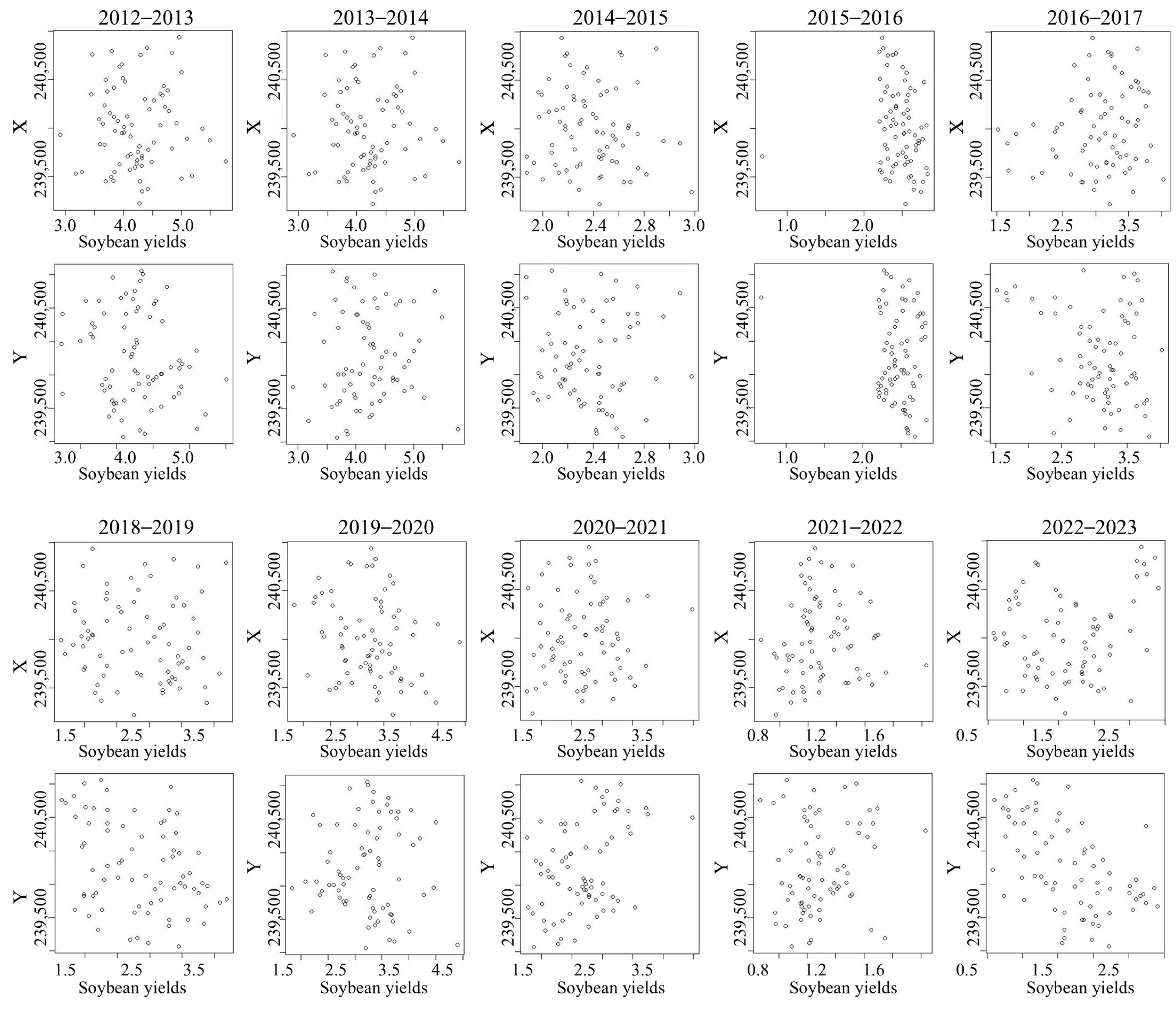
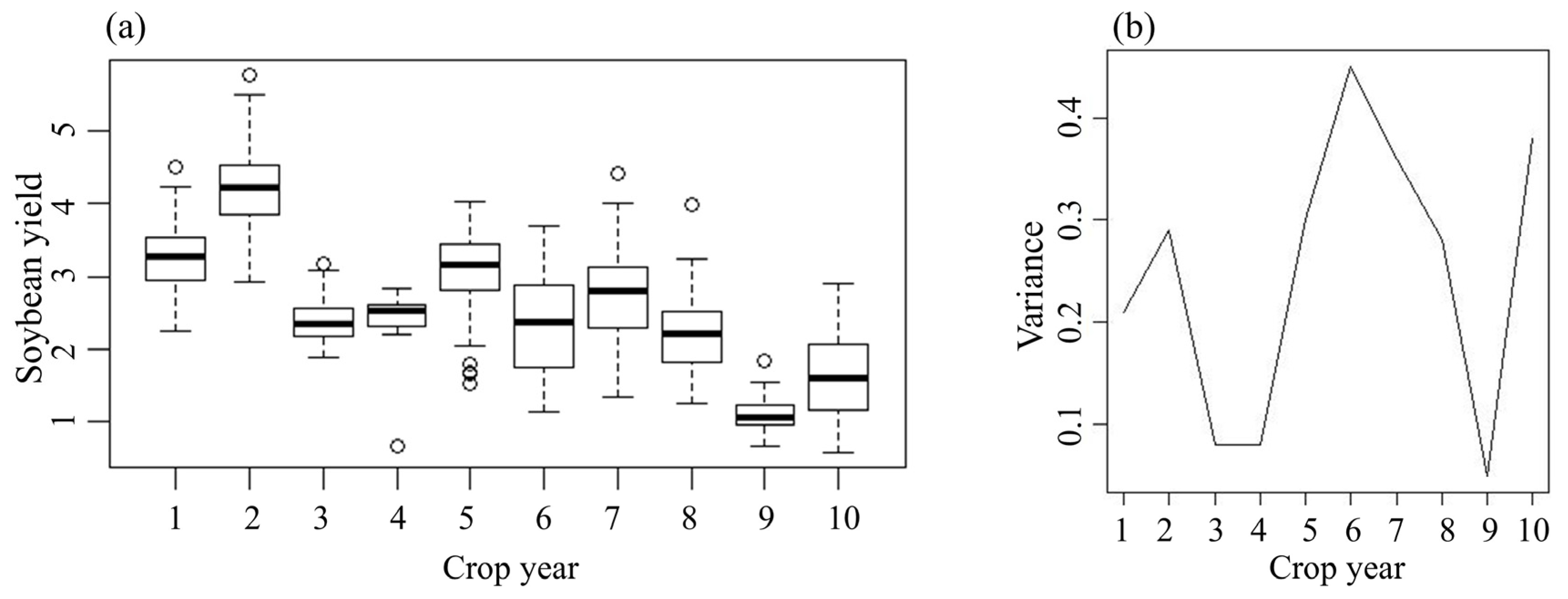
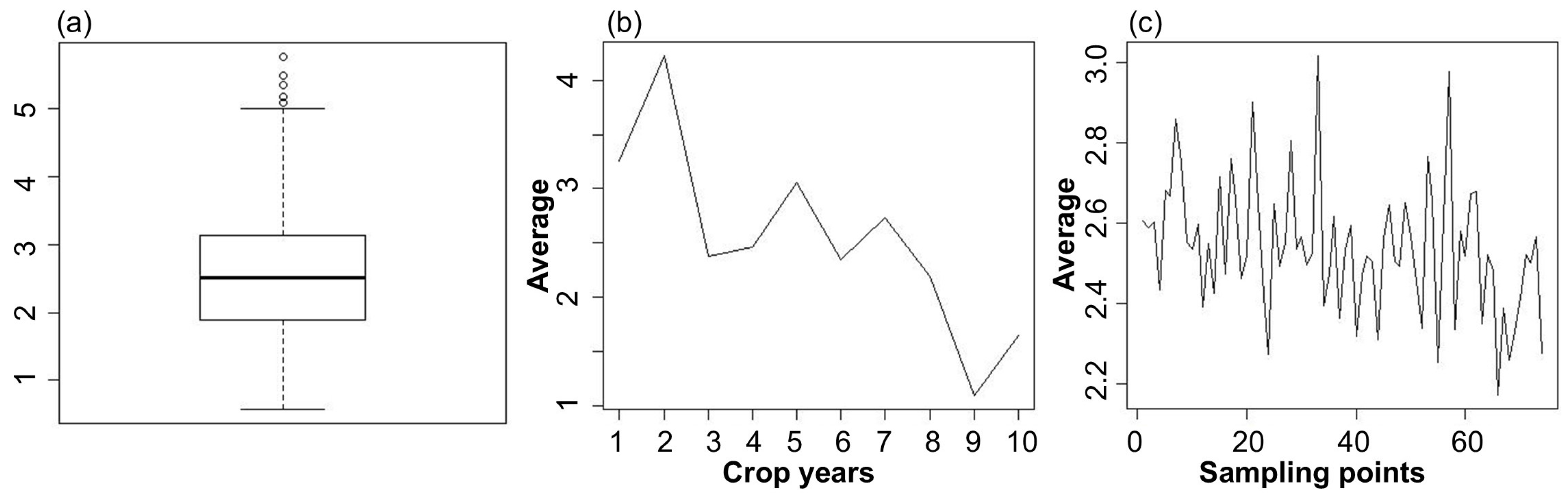
3.1. Descriptive Analysis of Soybean Yields

For most of the crop years, the soybean yield presented homogeneous data (CV ≤ 30), with the exception of the 2022–2023 crop year, which showed heterogeneity (CV > 30) (Table 1). Notably, the most homogeneous yields were observed in the 2014–2015 and 2015–2016 crop years (Table 1).

Table 1. Descriptive statistical table of soybean yield (t ha⁻¹) for each crop year.

Crop Year	Min.	Average	Max.	S.D	Var.	C.V (%)	Coef. X rp	Coef. Y rp	I Moran (p-Value)
2012–2013	2.24	3.26	4.51	0.46	0.21	14.20	−0.10 (0.37)	−0.19 (0.11)	0.36
2013–2014	2.91	4.23	5.77	0.54	0.29	12.81	0.01 (0.90)	0.09 (0.45)	0.71
2014–2015	1.87	2.38	3.18	0.28	0.08	11.76	−0.09 (0.43)	−0.02 (0.87)	0.11
2015–2016	0.67	2.46	2.83	0.28	0.08	11.21	−0.13 (0.26)	−0.15 (0.20)	0.05
2016–2017	1.52	3.06	4.03	0.55	0.30	17.91	0.17 (0.16)	−0.26 (0.03 *)	0.00
2018–2019	1.14	2.34	3.69	0.67	0.45	28.56	−0.07 (0.55)	−0.30 (0.004 *)	0.00
2019–2020	1.34	2.73	4.40	0.60	0.36	21.96	−0.22 (0.06)	0.01 (0.99)	0.00
2020–2021	1.26	2.18	3.99	0.53	0.28	24.28	0.03 (0.77)	0.41 (0.0003 *)	0.00
2021–2022	0.67	1.09	1.83	0.22	0.05	19.79	0.06 (0.61)	0.15 (0.20)	0.02
2022–2023	0.58	1.65	2.91	0.62	0.38	37.60	0.22 (0.06)	−0.53 (0.000001 *)	0.00

Min.: minimum value; Max.: maximum value; S.D: standard deviation; Var.: data variance (t² ha⁻¹); C.V (%): coefficient of variation; Coef. X and Coef. Y: Pearson’s linear correlation coefficient $\left(rp\right)$ of soybean yield data versus X and Y coordinates; * significant at 5% probability level; I Moran (p-value): spatial autocorrelation.

The minimum soybean yield was 0.58 t ha⁻¹, for the 2022–2023 crop year, while the maximum reached 5.77 t ha⁻¹, for the crop year 2013–2014 (Table 1). The lowest average soybean yield was observed in 2021–2022 at 1.09 t ha⁻¹, whereas the highest average yield occurred in 2013–2014, reaching 4.23 t ha⁻¹.

Also, the Moran test revealed that the soybean yield in the 2015–2016 crop year exhibits spatial dependence, indicating the suitability of a spatial modeling approach. The proximity matrix was constructed using the inverse Euclidean distance between the geographic coordinates of the sampling points (Table 1). Regarding the directional trend, the soybean yields (t ha⁻¹) from the 2018–2019, 2020–2021, and 2022–2023 crop years exhibited a moderate linear association with the Y-axis coordinates, with an $rp$ value exceeding 0.30. This relationship was confirmed by the significance test, yielding a p-value of < 0.05, leading to the rejection of the null hypothesis (H₀) at the 5% significance level. This indicates a significant correlation between the soybean yield and the Y-axis coordinates.

Additionally, the 2016–2017 crop year also presented a p-value of < 0.05, suggesting a correlation between the yield values and Y-axis coordinates, albeit a weak one, as its $rp$ value remained below 0.30 (Table 1). These directional trend patterns are further illustrated in Figure 4.

Figure 4. The graph of the dispersion of the X and Y axis coordinates with the values of the soybean yields of each crop year.

For most of the crop years, the soybean yield values varied across different locations, except for the 2018–2019 and 2022–2023 crop years, which exhibited more uniform distributions (Figure 5). The distributions for the 2015–2016 and 2016–2017 crop years were negatively skewed, whereas the remaining crop years displayed positive skewness (Figure 5). Some crop years also showed higher dispersion, and the observed trend in the mean values suggests that the process should not be considered independent (Figure 5a,b).

Figure 5. The boxplot of the soybean yield (t ha⁻¹) ($\circ$ outliers) (a) and the dispersion graph of the soybean yield variance (t ha⁻¹) (b) in the following crop years: 2012–2013 (1), 2013–2014 (2), 2014–2015 (3), 2015–2016 (4), 2016–2017 (5), 2018–2019 (6), 2019–2020 (7), 2020–2021 (8), 2021–2022 (9), and 2022–2023 (10).

The post plot graph (Figure 6) visualizes the spatial distribution of the soybean yield sampling points, with the colors representing yield values according to quartile-based intervals. The results indicate that the average soybean yield varied across the study area, with the highest yields typically concentrated in the southern or northern regions (Figure 6).

Figure 6. The post plot of the soybean yield (t ha⁻¹) in the following crop years: 2012–2013 (a), 2013–2014 (b), 2014–2015 (c), 2015–2016 (d), 2016–2017 (e), 2018–2019 (f), 2019–2020 (g), 2020–2021 (h), 2021–2022 (i), and 2022–2023 (j) ($\uparrow \mathbf{N}$ north direction).

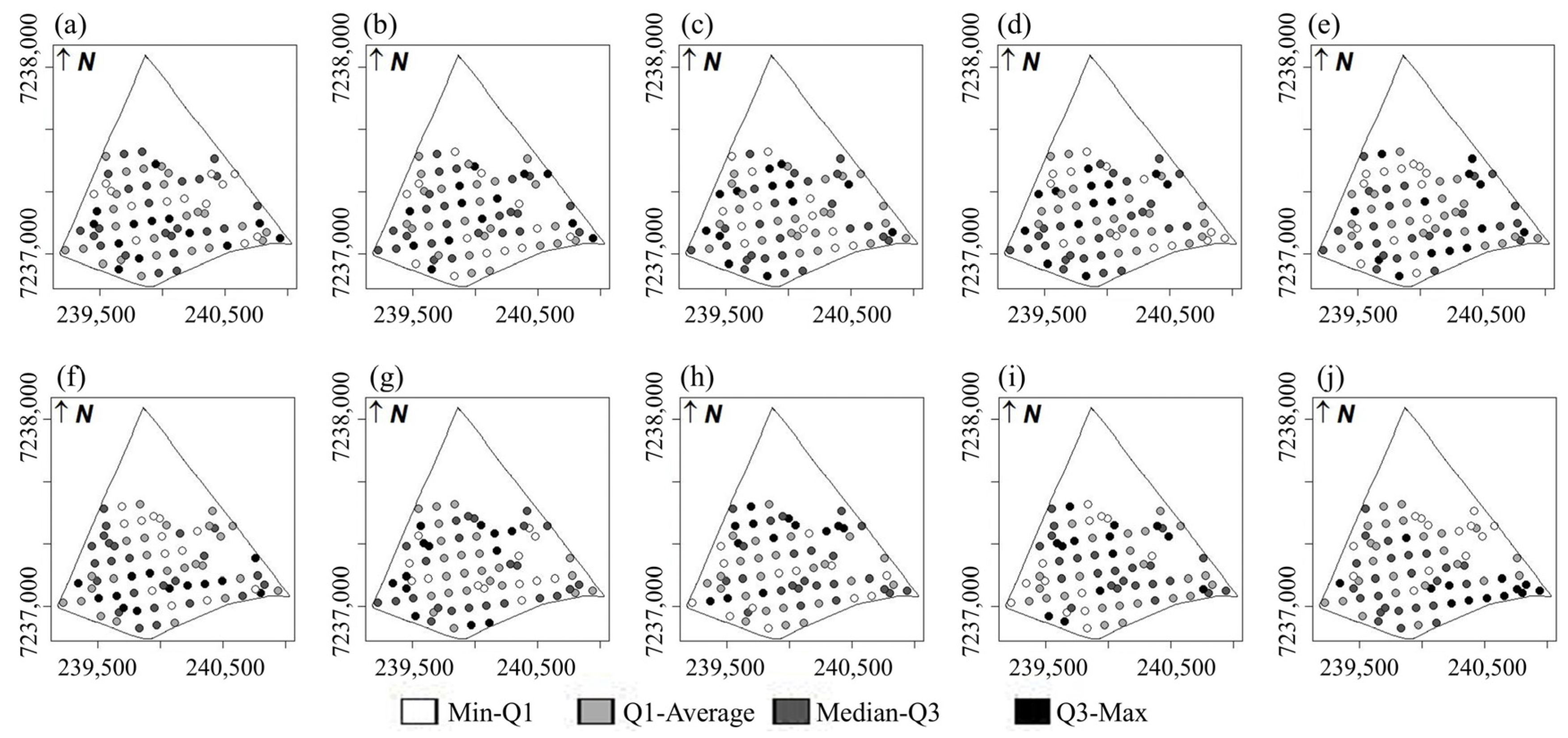
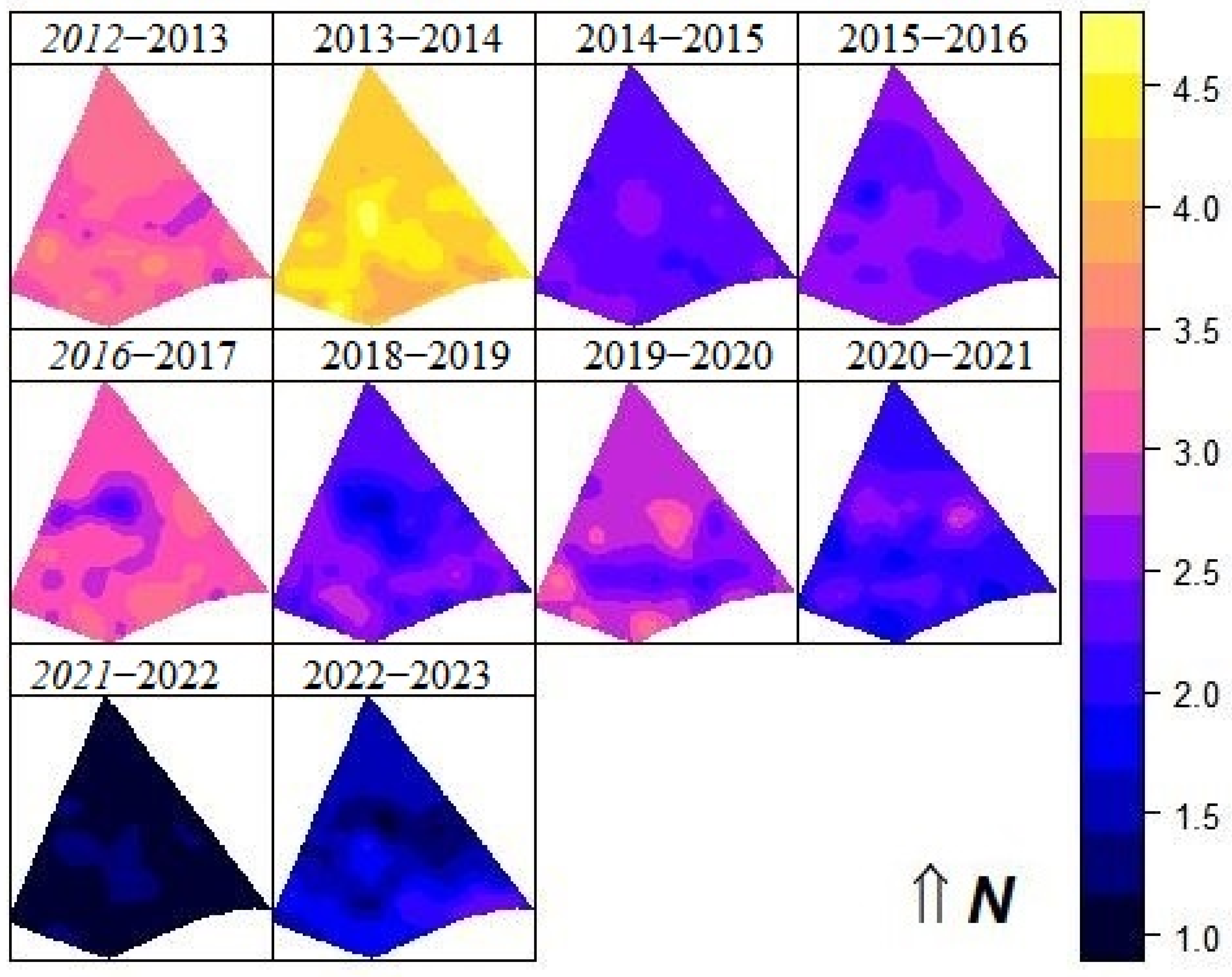
3.2. Spatio Temporal Analyses

Regarding the temporal correlations of the soybean yields, the Pearson’s linear correlation coefficients between each crop year (Table 2) show a statistically significant linear correlation (p-value < 0.05) for the following pairs: 2012–2013 and 2016–2017; 2013–2014 and 2015–2016; 2013–2014 and 2016–2017; 2013–2014 and 2018–2019; 2013–2014 and 2019–2020; 2013–2014 and 2022–2023; 2014–2015 and 2016–2017; 2014–2015 and 2021–2022; 2014–2015 and 2022–2023; 2015–2016 and 2018–2019; 2015–2016 and 2022–2023; 2019–2020 and 2020–2021; and 2020–2021 and 2021–2022. These correlations were assessed using Fisher’s z-transformation test. In contrast, the correlations between other crop years were not statistically significant (p-value > 0.05).

Table 2. The matrix of the temporal linear correlations between the crop years of the soybean yields.

Crop Year	2012–2013	2013–2014	2014–2015	2015–2016	2016–2017	2018–2019	2019–2020	2020–2021	2021–2022	2022–2023
2012–2013	1.00	0.29	−0.16	−0.12	−0.05	0.19	−0.08	−0.15	−0.07	0.09
2013–2014	0.29	1.00	−0.07	−0.04	0.00	0.01	0.01	0.14	−0.13	−0.02
2014–2015	−0.16	0.07	1.00	0.59	0.02	−0.07	0.38	−0.05	0.06	−0.01
2015–2016	−0.12	−0.04	0.59	1.00	0.17	0.04	0.17	−0.26	0.12	−0.05
2016–2017	−0.05	0.00	0.02	0.17	1.00	0.28	−0.20	−0.13	0.15	0.39
2018–2019	0.19	0.01	−0.07	0.04	0.28	1.00	−0.17	−0.25	−0.12	0.30
2019–2020	−0.08	0.01	0.38	0.17	−0.20	−0.17	1.00	−0.05	−0.08	−0.08
2020–2021	−0.15	0.14	−0.05	−0.26	−0.13	−0.25	−0.05	1.00	0.03	−0.25
2021–2022	−0.07	−0.13	0.06	0.12	0.15	−0.12	−0.08	0.03	1.00	−0.07
2022–2023	0.09	−0.02	−0.01	−0.05	0.39	0.30	−0.08	−0.25	−0.07	1.00

Considering the study of the 74 georeferenced sampling points during the period of 10 crop years in the same area (2012–2013 to 2022–2023), the average soybean yield was 2.54 t ha⁻¹, presenting the heterogeneity of its values in relation to the average (CV > 30%) (Table 3).

Table 3. The descriptive statistics of the soybean yield values (t ha⁻¹) at the 74 sampling points during the 10-crop-year study (2012–2013 to 2022–2023).

Statistics	nT	Min.	Average	Max.	S.D	Var.	C.V (%)	Coef. X (rp)	p-Value	Coef. Y (rp)	p-Value
Overall soybean yield	740	0.58	2.54	5.77	0.96	0.92	37.83	−0.01 NS	0.94	−0.05 NS	0.14

Min.: minimum value; Max.: maximum value; S.D: standard deviation; Var.: data variance; C.V (%): coefficient of variation; Coef. X and Coef. Y: Pearson’s linear correlation coefficient (rp) of data versus X and Y coordinates, respectively; NS: not significant at 5% probability level.

The soybean yield did not show a directional trend with respect to the X and Y coordinates (Table 3). The significance test results show that the correlation between the soybean yield and both the X and Y coordinates has p-values of greater than 0.05. This indicates that the null hypothesis that the linear correlation is zero is not rejected $(H_0:\rho =0)$ at the level of 5% significance; that is, there is no significant linear correlation between the soybean yield and the X and Y axis coordinates; consequently, there is no directional trend (Table 3).

The average soybean yield across all the crop years continued to exhibit variability, with disparate data points (Figure 7a).

Figure 7. Boxplot of overall soybean yield (t ha⁻¹) ($\circ$ outliers) (a), temporal average (b), and spatial average (c) of soybean yield (t ha⁻¹), considering all crop years.

The temporal average of the soybean yield (t ha⁻¹), considering all the spatial locations, shows the nature of and variations in the soybean yields over the crop years (Figure 7b). Notably, a peak can be observed for the 2013–2014 crop year and a great fall for the 2021–2022 crop year (Figure 7b). As for the spatial average of the soybean yield, considering all the crop years, it can be seen that there is variation in the values of these productivities at the sampling points of the area under study (Figure 7c).

3.3. Gaussian Linear Spatial Model Analysis with Multiple Independent Repetitions (${\mathit{\Sigma }}_{\mathit{T}\mathit{S}}={\mathit{\Sigma }}_{\mathit{T}}\otimes {\mathit{\Sigma }}_{\mathit{S}}$, Considering ${\mathit{\Sigma }}_{\mathit{T}}={\mathit{I}}_{\mathit{T}}$ and ${\mathit{\Sigma }}_{\mathit{S}}={\phi }_1{I}_n+{\phi }_2{R}_S\left({\phi }_3\right))$

Considering all the points sampled ($n$ = 74) in all the crop years ($T$ = 10), the best adjusted model was the Matérn, with a smoothing parameter of k = 1 (Table 4), according to the criteria of AIC, BIC, cross-validation, and trace.

Table 4. The estimates obtained by ML of the parameters of the chosen model, Matérn, with k = 1, for the covariance structure of the soybean yield, considering all the crop years (asymptotic standard errors in parentheses).

$\widehat{\mathit{\mu }}$	${\widehat{\mathit{\phi }}}_1$	${\widehat{\mathit{\phi }}}_2$	${\widehat{\mathit{\phi }}}_3$	$\widehat{\mathit{\alpha }}$
2.5357 (0.0343)	0.3142 (0.2405)	0.2526 (0.2439)	74.5948 (52.8771)	298.2691

$\widehat{\mathit{\mu }}:$ estimated mean; ${\widehat{\mathit{\phi }}}_1$: estimated nugget effect; ${\widehat{\mathit{\phi }}}_2:$ estimated contribution; ${\widehat{\mathit{\phi }}}_3$: estimated range function; $\widehat{\mathit{\alpha }}$: estimated practical range.

Figure 8 shows the distribution of the soybean yield, considering the structure of the Gaussian linear spatial model with multiple independent repetitions for each crop year (${\mathit{\Sigma }}_{\mathit{T}}={\mathit{I}}_{10})$. The same behaviors of the individual soybean yield maps of each crop year were observed, presenting the highest soybean yields in the crop year 2013–2014 and the lowest in the crop years 2021–2022 and 2022–2023, with adverse weather possibly having affected soybean production. Also, for the crop years 2012–2013, 2016–2017, 2018–2019, and 2022–2023, the highest values for the soybean yield were found in the southern region of the study area, while the lowest values were in the central region (Figure 8). For the 2015–2016 crop year, the lowest values of the soybean yield were scattered in the southern and northern regions (Figure 8). For the years 2013–2014, 2014–2015, and 2019–2020, the lowest values of the soybean yield were located in the southern region, while for the 2020–2021 and 2021–2022 crop years, the highest values for the soybean yield were in the central region.

Figure 8. The map of the soybean yields (t ha⁻¹), considering the Gaussian linear spatial model with independent multiple repetitions, for the following crop years: 2012–2013, 2013–2014, 2014–2015, 2015–2016, 2016–2017, 2018–2019, 2019–2020, 2020–2021, 2021–2022, and 2022–2023 ($\uparrow \mathbf{N}$ north direction).

3.4. Model with Separable Covariance Structure (${\mathit{\Sigma }}_{\mathit{T}\mathit{S}}={\mathit{\Sigma }}_{\mathit{T}}\otimes {\mathit{\Sigma }}_{\mathit{S}}$, Considering ${\mathit{\Sigma }}_{\mathit{T}}={\mathit{R}}_{\mathit{T}}\left({\mathit{\phi }}_4\right)$ and ${\mathit{\Sigma }}_{\mathit{S}}={\phi }_1{I}_n+{\phi }_2^{*}{R}_S\left({\phi }_3\right))$

Considering all the points sampled ($n$ = 74) in all the crop years ($T$ = 10), the best adjusted model for ${\mathit{\Sigma }}_{\mathit{T}}$ e ${\mathit{\Sigma }}_{\mathit{S}}$ was the Matérn family, with a smoothing parameter of k = 0.5 (exponential), according to the criteria of the cross-validation and the trace. The fixed parameter ${\phi }_3$ was 120 m from the previous analysis (the geostatistical analysis of individual soybean yields) (Table 5).

Table 5. The estimates obtained by ML of the parameters of the chosen model, the Matérn family, with k = 0.5, using the EM algorithm (standard asymptotic errors in parentheses).

$\widehat{\mathit{\mu }}$	${\widehat{\mathit{\phi }}}_1$	${\widehat{\mathit{\phi }}}_2$	${\widehat{\mathit{\phi }}}_4$
2.5310 (0.0607)	0.5088 (0.4445)	0.0048 (0.0005)	0.4924 (0.0529)

$\widehat{\mu }:$ estimated mean; ${\widehat{\phi }}_1$: estimated nugget effect; ${\widehat{\phi }}_2^{*}={\displaystyle \frac{{\phi }_2}{{\left({\phi }_3\right)}^{2\kappa }}}:$ estimated contribution; ${\widehat{\phi }}_4$: the estimated time parameter of the Matérn family model, with the smoothing parameter k = 0.5.

Table 6 shows the values of the root mean square error, and the lower the value, the better the model performed. Therefore, by comparing the observed values with the predicted values, by RMSE, it can be seen that the lowest value was presented for the 2020–2021 crop year.

Table 6. The root mean square error values of the model for each crop year.

RMSE	2012–2013	2013–2014	2014–2015	2015–2016	2016–2017	2018–2019	2019–2020	2020–2021	2021–2022	2022–2023
	0.5590	1.0427	0.2494	0.2353	0.5366	0.5621	0.2574	0.2329	0.8359	0.6877

The RMSE = $\sqrt{\sum _{i=1}^n{\displaystyle \raisebox{1ex}{${({\widehat{y}}_i-y_i)}^2$}\!\left/ \!\raisebox{-1ex}{$n$}\right.}}$, where ${\widehat{y}}_1, \dots , {\widehat{y}}_n$ are predicted values; $y_1, \dots , y_n$ are observed values; and n is the number of observations.

Thus, the covariance matrix is given by ${\widehat{\mathit{\Sigma }}}_{\mathit{T}\mathit{S}}=R_T\left(0.4924\right)⨂(0.5088\ast I_{74}+0.0048R_S\left(120\right))$, being

$$R_T\left(0.4924\right)={\displaystyle \frac{1}{\Gamma \left(0.5\right)}}{\left({\displaystyle \frac{u_t}{0.4924}}\right)}^{0.5}{K}_{0.5}\left({\displaystyle \frac{u_t}{0.4924}}\right), \mathrm{t}=1,\dots ,\mathrm{T}, u_t>0$$

$${\mathit{R}}_{\mathit{S}}\left(120\right)=\left\{\begin{array}{c}1, se i=j \\ {\displaystyle \frac{1}{\Gamma \left(0.5\right)}}\left({120\delta }_{ij}\right)K_{0.5}\left({\displaystyle \frac{{\delta }_{ij}}{120}}\right), se i\ne je{\delta }_{ij}>0\end{array}\right.$$

where $i,j=1,\dots ,n$, ${\delta }_{ij}$ is the euclidean distance between $i$ locations, and $j$ and $u_t=\left|t_l-t_m\right|,l,m=1,\dots ,T.$

Analyzing the semivariogram in the temporal sense, an oscillation of the semivariance values is observed with the increase in the temporal distances. When analyzing in the spatial sense, we can see a more evident increase in the semivariance values for the first spatial lags with a rapid stabilization, indicating a low radius of spatial dependence (Figure 9).

Figure 9. Three-dimensional semivariogram.

Figure 10 shows the distribution of the soybean yield for each crop year, considering the model with a separable covariance structure $\left({\widehat{\mathit{\Sigma }}}_{\mathit{T}\mathit{S}}\right)$. The highest soybean yield was recorded in the 2013–2014 crop year, whereas the lowest yields were observed in 2021–2022 and 2022–2023.

Figure 10. The map of the soybean yields (t ha⁻¹), considering the linear spatial model with separable covariance structures, for the following crop years: 2012–2013, 2013–2014, 2014–2015, 2015–2016, 2016–2017, 2018–2019, 2019–2020, 2020–2021, 2021–2022, and 2022–2023 ($\uparrow \mathbf{N}$ north direction).

Also, for the crop years 2012–2013, 2013–2014, and 2016–2017, the highest values for the soybean yield are found in the southern region of the study area, while the lowest values are in the central region (Figure 10). The 2014–2015 and 2015–2016 crop years showed little variation in soybean yield values in the area. For the crop year 2018–2019, the lowest values of soybean yield are located in the central region, and the highest yields are located in the southwest region of the area. In the 2019–2020 crop year, soybean production was highest in the central and southwest regions of the study area. In contrast, during the 2020–2021, 2021–2022, and 2022–2023 crop years, the highest yields were concentrated in the south–central region.

Overall, for the last five crop years, the findings largely align with the producer’s practical survey, confirming the observed yield patterns in the study area.

Figure 11 and Table 7 show a comparative analysis of the thematic maps of the soybean yield, considering both the spatiotemporal model with a separable covariance structure and the Gaussian linear spatial model with multiple independent repetitions. The estimated values of Global-GA’s inaccuracies were lower than 0.85, and the concordance indices, the Kp’s and Kpw’s, were lower than 0.67 for all the crop years, suggesting notable differences in the spatial patterns captured by each model.

Figure 11. The map of the soybean yields (t ha⁻¹), considering the Gaussian linear spatial model with multiple independent repetitions and the spatial time model with separable covariance structures, for the following crop years: 2012–2013, 2013–2014, 2014–2015, 2015–2016, 2016–2017, 2018–2019, 2019–2020, 2020–2021, 2021–2022, and 2022–2023 ($\uparrow \mathbf{N}$ north direction).

Table 7. The estimated values of the Similarity Measures Global Accuracy (GA), Kappa (K_p), and weighted Kappa (K_pw) metrics, comparing the maps generated considering the Gaussian linear spatial model with multiple independent repetitions and the spatiotemporal model with separable covariance structures for the following crop years: 2012–2013, 2013–2014, 2014–2015, 2015–2016, 2016–2017, 2018–2019, 2019–2020, 2020–2021, 2021–2022, and 2022–2023.

Crop Years/Index	GA	Kp	Kpw
2012–2013	0.0131	−0.0299	0.0880
2013–2014	0.0000	−0.0006	0.0290
2014–2015	0.1702	−0.1043	0.3238
2015–2016	0.5180	0.1087	0.2571
2016–2017	0.0639	−0.0124	0.1453
2018–2019	0.4001	0.0798	0.4499
2019–2020	0.3981	0.0886	0.4230
2020–2021	0.1471	−0.0208	0.1694
2021–2022	0.0000	−0.2500	0.0006
2022–2023	0.0350	−0.0301	0.1061

The GA of < 0.85 and the Kp and Kpw of < 0.67 indicate that the maps are dissimilar; that is, they present low accuracy between the maps generated by the two methods.

This study brings a benefit to precision agriculture as it makes it possible to analyze the variable of interest both in space and in time, which helps in the demand for guidance in making decisions regarding soil management practices, such as for future indications of localized applications.

4. Discussion

It is worth remembering that the data quality and the elimination of possible errors in data collection are extremely important for the consistency of the results presented by the models and their accuracy.

It was observed that, for most crop years, the average soybean productivity was considered low in relation to the state and national productivity levels [40], except for the 2012–2013 crop year, which presented high productivity in relation to the national productivity (2.938 t ha⁻¹) and low productivity in relation to the state productivity (3.348 t ha⁻¹). The 2013–2014 crop year presented high productivity in relation to the national (2.854 t ha⁻¹) and state (2.950 t ha⁻¹) productivity [40]. Working with similar sample points [41], we also found that for the 2020–2021 crop year, the average soybean productivity was lower than the national and state productivity. This variation in the average soybean productivity throughout the crop years is influenced by several factors, mainly by climatic factors, such as an excess or lack of rainfall; these climate interactions can indicate the best periods for planting and harvesting soybeans [42].

For most of the agricultural years, the soybean productivity presented homogeneous data (CV ≤ 30); that is, the soybean productivity values were less dispersed in relation to the average productivity [43].

Regarding the directional trend, most of the crop years did not show a linear association between the respective soybean productivity values and the X or Y axis coordinates, with $rp$ values of lower than 0.30 [44].

There was a peak in soybean productivity for the 2013–2014 crop year, and a large drop in productivity for the 2021–2022 crop year. This fact can be explained by climatic conditions. The influence of the La Niña phenomenon in the 2021–2022 crop year in the southern region of the country, for example, caused a drastic reduction in rainfall in November and December 2021, being a determining factor in the reduction in productivity [40].

The temporal averages of soybean productivity in each location are important because they allow the interpretation of the soybean production over the years [45].

A comparative study of the thematic maps of the soybean yield constructed by performing an individual analysis year by year with the Gaussian linear spatial model with multiple independent repetitions verified the estimated value of the Global Accuracy Index, GA, of higher than 0.85, indicating that the maps are similar [37]. Furthermore, the values of the Kappa, K_p, and weighted Kappa, K_pw, concordance indices indicated high accuracy between the maps generated by the two methods, with values of greater than 0.80 [38].

A visual assessment reveals that the thematic maps of the soybean yield, generated using the spatiotemporal model with a separable covariance structure and the Gaussian linear spatial model with multiple independent repetitions, do not exhibit similarity (Figure 11).

This discrepancy is confirmed by the low accuracy index values (GA < 0.85 and K_p, K_pw < 0.67) [37,38], indicating that the maps differ in their representation of the soybean yield distribution across the study area. These differences suggest that the soybean yield was influenced by temporal factors over the years. Additionally, it is observed that the temporal component leads to a smoothing effect over time, producing more-homogenized maps with fewer segmented areas. Despite this, a temporal trend remains perceptible in the distribution patterns (Figure 11).

5. Conclusions

This analysis of soybean yields over ten crop years (2012–2013 to 2021–2022) revealed significant temporal and spatial variability. The lowest average yield was recorded in the 2021–2022 crop year, whereas the highest yield occurred in 2013–2014. These variations highlight the influence of climatic conditions and other environmental factors on soybean productivity over time.

A comparative evaluation of the thematic maps generated using the Gaussian linear spatial model with multiple independent repetitions and the spatiotemporal model with a separable covariance structure demonstrated that the latter provides a more informative and comprehensive analysis. The spatiotemporal model accounts for both the spatial and temporal dependencies, offering a more detailed representation of the soybean yield distribution.

Furthermore, the presence of spatial trends in the data reinforces the suitability of the spatiotemporal model. While the Gaussian linear spatial model captures independent spatial variations for each crop year, it does not incorporate temporal correlations, potentially overlooking key patterns related to yield evolution. The separable covariance structure, on the other hand, provides a refined framework that integrates spatial and temporal dependencies, reducing uncertainties and improving predictive capabilities.

Additionally, the analysis confirmed that the soybean yield exhibited spatial dependence in certain crop years, justifying the application of geostatistical methods. The findings also indicate that temporal trends tend to smooth yield distributions over time, further supporting the need for an integrated spatiotemporal modeling approach. In conclusion, incorporating a spatiotemporal model with a separable covariance structure enhances the accuracy and interpretability of soybean yield analyses, making it a more effective tool for decision-making in precision agriculture.

This article presented a limitation regarding the application of a formal separability test, due to the limited temporal extension of our dataset (10 crop years); however, we decided to work with space–time separability to overcome the computational complexity of non-separable models.

Future research will focus on extending the dataset to include additional crop years, which will allow for a more robust analysis of long-term trends. Expanding the temporal scope will also enable the application of non-separable covariance structures, which may provide a more flexible and accurate representation of spatiotemporal dependencies. This advancement will be essential for refining predictive models and improving agricultural decision-making strategies.

References

- Lima, V.A.; Dos Santos, I.C. Atividades de inovação em agricultura de precisão no Brasil e o longo caminho para o ODS 2. Rev. Electrónica Mens. 2019, 3, 1–15. [Google Scholar]
- Barbosa, D.P.; Bottega, E.L.; Valente, D.S.M.; Santos, N.T.; Guimarães, W.D.; Ferreira, M.D.P. Influence geometric anisotropy in management zones delineation. Rev. Ciênc. Agron. 2019, 50, 543–551. [Google Scholar]
- Noetzold, R.; Da Silva, L.M.; Schoninger, E.L.; Tomé, P.C.D.T.; Alves, M.C. Variabilidade espacial e temporal de atributos químicos do solo durante cinco safras. Rev. Bras. Geom. 2018, 6, 328–345. [Google Scholar] [CrossRef]
- Ortega, R.A.; Santibanez, O.A. Determination of management zones in corn (Zea mays L.) based on soil fertility. Comput. Electron. Agric. 2007, 58, 49–59. [Google Scholar] [CrossRef]
- Cressie, N. Comment on “an approach to statistical spatial-temporal modeling of meteorological fields” by m. s. handcock and j. r. wallis. J. Am. Stat. Assoc. 1994, 89, 379–382. [Google Scholar]
- Goodall, C.; Mardia, K.V. Challenges in multivariate spatio-temporal modeling. In Proceedings of the XVII-th International Biometric Conference, Hamilton, ON, Canada, 8–12 August 1994; Volume 39, pp. 1–17. [Google Scholar]
- Cressie, N.; Shi, T.; Kang, E.L. Fixed rank filtering for spatio-temporal data. J. Comput. Graph. Stat. 2010, 19, 724–745. [Google Scholar] [CrossRef]
- Cressie, N.; Wikle, C.K. Statistics for Spatio-Temporal Data; John Wiley & Sons: Hoboken, NJ, USA, 2011; p. 585. [Google Scholar]
- De Bastiani, F.; Galea, M.; Cysneiros, A.H.M.A.; Uribe-Opazo, M.A. Gaussian spatial linear models with repetitions: An application to soybean productivity. Spat. Stat. 2017, 21, 319–335. [Google Scholar] [CrossRef]
- Zhuo, Z.; Xing, A.; Li, Y.; Huang, Y.; Nie, C. Spatio-temporal variability and the factors influencing soil-available heavy metal micronutrients in different agricultural sub-catchments. Sustainability 2019, 11, 5912. [Google Scholar]
- Yang, H.; Song, X.; Zhao, Y.; Wang, W.; Cheng, Z.; Zhang, Q.; Cheng, D. Temporal and spatial variations of soil C, N contents and C: N stoichiometry in the major grain-producing region of the North China Plain. PLoS ONE 2021, 16, e0253160. [Google Scholar]
- Saavedra-Nievas, J.C.; Nicolis, O.; Galea, M.; Ibacache-Pulgar, G. Influence diagnostics in gaussian spatial–temporal linear models with separable covariance. Environ. Ecol. Stat. 2023, 30, 131–155. [Google Scholar]
- Santos, H.G.; Jacomine, P.T.; Anjos, L.H.C.; Oliveira, V.A.; Lumbreras, J.F.; Coelho, M.R.; Araujo Filho, J.O.; Oliveira, J.B.; Cunha, T.J.F. Brazilian Soil Classification System, 5th ed.; Embrapa: Brasília, Brazil, 2018. [Google Scholar]
- Aparecido, L.; Rolim, G.S.; Richetti, J.; Souza, P.S.; Johann, J.A. Köppen, Thornthwaite and Camargo climate classifications for climatic zoning in the State of Paraná, Brazil. Ciênc Agrotecnologia 2016, 40, 405–417. [Google Scholar] [CrossRef]
- Chipeta, M.G.; Terlouw, D.J.; Phiri, K.S.; Diggle, P.J. Inhibitory geostatistical designs for spatial prediction taking account of uncertain covariance structure. Environmetrics 2017, 28, e2425. [Google Scholar] [CrossRef]
- Maltauro, T.C.; Guedes, L.P.C.; Uribe-Opazo, M.A.; Canton, L.E.D. Spatial multivariate optimization for a sampling redesign with a reduced sample size of soil chemical properties. Rev. Bras. Ciênc. Solo 2023, 47, e0220072. [Google Scholar] [CrossRef]
- Arruda, M.R.; Moreira, A.; Pereira, J.C.R. Amostragem e Cuidados na Coleta de Solo Para Fins de Fertilidade; Embrapa Amazônia Ocidental Manaus: Itacoatiara, Brazil, 2014. [Google Scholar]
- Walkley, A.; Black, I.A. An examination of the Degtjareff method for determining soil organic matter and a proposed modification of the chromic acid titration method. Soil Sci. 1934, 37, 29–38. [Google Scholar] [CrossRef]
- Mardia, K.V.; Marshall, R.J. Maximum likelihood estimation of models for residual covariance in spatial regression. Biometrika 1984, 71, 135–146. [Google Scholar] [CrossRef]
- Uribe-Opazo, M.A.; Borssoi, J.A.; Galea, M. Influence diagnostics in Gaussian spatial linear models. J. Appl. Stat. 2012, 39, 615–630. [Google Scholar] [CrossRef]
- Uribe-Opazo, M.A.; Dalposso, G.H.; Galea, M.; Johann, J.A.; De Bastiani, F.; Moyano, E.N.C.; Grzegozewski, D.M. Spatial variability of wheat yield using the gaussian spatial linear model. Aust. J. Crop Sci. 2023, 17, 179–189. [Google Scholar] [CrossRef]
- De Bastiani, F.; Cysneiros, A.H.M.A.; Uribe-Opazo, M.A.; Galea, M. Influence diagnostics in elliptical spatial linear models. Sociedad de Estadística e Investigación Operativa. TEST 2015, 24, 322–340. [Google Scholar] [CrossRef]
- Silva, A.S.; Ribeiro Jr, P.J. Modelos gaussianos geoestatísticos espaço-temporais e aplicações. Rev. Mat. Estat. 2000, 20, 1–10. [Google Scholar]
- Finkenstadt, B.; Held, L.; Isham, V. Statistical Methods for Spatio-Temporal Systems, 1st ed.; Chapman and Hall/CRC: New York, NY, USA, 2006; p. 286. [Google Scholar]
- Gneiting, T.; Genton, M.G.; Guttorp, P. Geostatistical space-time models, stationarity, separability, and full symmetry. Monogr. Stat. App. Probab. 2006, 107, 151. [Google Scholar]
- Matérn, B. Spatial Variation, 2nd ed.; Lecture Notes in Statistics; Springer: Berlin/Heidelberg, Germany, 1986. [Google Scholar]
- Diggle, P.J.; Giorgi, E. Model-Based Geostatistics for Global Public Health: Methods and Applications, 1st ed.; Chapman and Hall/CRC: New York, NY, USA, 2019; p. 274. [Google Scholar]
- Cappello, C.; De Iaco, S.; Posa, D. Testing the type of non-separability and some classes of space-time covariance function models. Stoch Environ. Res Risk. Assess 2018, 32, 17–35. [Google Scholar] [CrossRef]
- Uribe-Opazo, M.A.; De Bastiani, F.; Galea, M.; Schemmer, R.C.; Assumpção, R.A.B. Influence diagnostics on a reparameterized t-Student spatial linear model. Spat. Stat. 2021, 41, 100481. [Google Scholar] [CrossRef]
- Zhang, H. Inconsistent estimation and asymptotically equal interpolations in model-based geostatistics. J. Am. Stat. Assoc. 2004, 99, 250–261. [Google Scholar] [CrossRef]
- Zhang, H.; Zimmerman, D.L. Hybrid estimation of semivariogram parameters. Math. Geol. 2007, 39, 247–260. [Google Scholar] [CrossRef]
- Zhang, H.; El-Shaarawi, A. On spatial skew-gaussian processes and applications. Environmetrics 2010, 21, 33–47. [Google Scholar] [CrossRef]
- Stein, M.L. (Ed.) Interpolation of Spatial Data: Some Theory for Kriging; Springer Science & Business Media: Berlin/Heidelberg, Germany, 1999. [Google Scholar]
- Lange, K.L.; Little, R.J.A.; Taylor, J.M.G. Robust statistical modeling using the t distribution. J Am Stat Assoc 1989, 84, 881–896. [Google Scholar] [CrossRef]
- Mitchell, A.F.S. The information matrix, skewness tensor and α-connections for the general multivariate elliptic distribution. Ann. Inst. Stat. Math. 1989, 41, 289–304. [Google Scholar] [CrossRef]
- Landim, P.M.B. Sobre Geoestatística e mapas. Terra E Didat. 2006, 2, 19–33. [Google Scholar] [CrossRef]
- Anderson, J.F.; Hardy, E.E.; Roach, J.T.; Witmer, R.E. A Land Use and Land Cover Classification System for Use with Remote Sensor Data; Government Print Office: Alexandria, VA, USA, 2001. [Google Scholar]
- Krippendorff, K. Content Analysis: An Introduction to Its Methodology, 2nd ed.; Sage Publications Ltd.: Thousand Oaks, CA, USA, 2013. [Google Scholar]
- R Development Core Team. R: A Language and Environment for Statistical Computing; R Foundation for Statistical Computing: Vienna, Austria, 2024; Available online: https://www.R-project.org/ (accessed on 5 January 2024).
- CONAB—Companhia Nacional de Abastecimento. Séries Históricas: Soja Brasil—Safras 1976/1977 a 2024/2025. Available online: https://www.conab.gov.br/info-agro/safras/serie-historica-das-safras?start=30 (accessed on 5 January 2025).
- Dalposso, G.H.; Uribe-Opazo, M.A.; De Oliveira, M.P. Comparison between Matheron and Genton semivariance function estimators in spatial modeling of soybean yield. Aust. J. Crop Sci. 2022, 16, 916–921. [Google Scholar] [CrossRef]
- Gasparin, P.P.; da Silva, E.M.; Becker, W.R.; Paludo, A.; Guedes, L.P.C.; Johann, J.A. Agroclimatic and spectral regionalization for soybean in different agricultural settings in the state of Paraná, Brazil. J. Agric. Sci. 2024, 162, 291–306. [Google Scholar] [CrossRef]
- Pimentel-Gomes, F.; Garcia, C.H. Estatística Aplicada a Experimentos Agronômicos e Florestais; FEALQ: Piracicaba, Brazil, 2002. [Google Scholar]
- Callegari-Jacques, S.M. Bioestatística: Princípios e Aplicações; Artmed: Porto Alegre, Brasil, 2003. [Google Scholar]
- Wikle, C.K.; Zammit-Mangion, A.; Cressie, N. Spatio-Temporal Statistics with R; CRC Press; Taylor & Francis Group: Boca Raton, FL, USA, 2019; p. 380. [Google Scholar]
Disclaimer/Publisher’s Note: The statements, opinions and data contained in all publications are solely those of the individual author(s) and contributor(s) and not of MDPI and/or the editor(s). MDPI and/or the editor(s) disclaim responsibility for any injury to people or property resulting from any ideas, methods, instructions or products referred to in the content. |
© 2025 by the authors. Licensee MDPI, Basel, Switzerland. This article is an open access article distributed under the terms and conditions of the Creative Commons Attribution (CC BY) license (https://creativecommons.org/licenses/by/4.0/).