Coupling Coordination Development Between Cultivated Land and Agricultural Water Use Efficiency in Arid Regions: A Case Study of the Turpan–Hami Basin

Abstract

The coupling coordination relationship between cultivated land and water resources in arid regions is crucial for ecological security and sustainable food production. This study explores the interaction between these resources to optimize the allocation of water–land resources, ecological resources, and agricultural resources and promote synergistic development. Taking the Turpan–Hami Basin as a case study, this research analyzed the utilization efficiency of cultivated land and agricultural water resources from 2000 to 2023 using a super-efficiency SBM-DEA model. A coupling coordination degree model was constructed to evaluate their coordinated development level, with spatial autocorrelation and other methods used to examine spatiotemporal patterns. Key findings include: (1) The overall utilization efficiency of both resources was relatively low, with mean values of 0.516 and 0.596, showing a fluctuating upward trend and significant spatial heterogeneity; (2) The mean coupling coordination degree (CCD) ranked as follows: Barkol Kazakh Autonomous County (0.587) > Yiwu County (0.563) > Gaochang District (0.494) > Shanshan County (0.437) > Tuokexun County (0.417) > Yizhou District (0.342), with an annual growth rate of 4.6%; (3) Regional disparities were dominated by intra-regional differences (42.0%), followed by transvariation density (30.64%). This study provides scientific evidence for optimizing resource allocation in arid regions.

1. Introduction

As critical components of ecosystems, the coordinated development of water and soil resources plays a vital role in advancing ecosystem sustainability [1]. Climate warming and intensified human activities have heightened ecological pressures, exacerbating the conflict between cultivated land and water scarcity in arid regions, which has emerged as a major threat to food security and ecological balance [2]. The report of the 20th National Congress of the Communist Party of China explicitly emphasized the need to comprehensively strengthen food security foundations, enforce joint governmental responsibility for food security, strictly maintain the 1.8 billion mu (≈120 million hectares) cultivated land redline, and coordinate the management of water resources, water environments, and aquatic ecosystems to promote ecological conservation in major rivers and lakes [3]. Currently, China faces tight food security conditions, with cultivated land and water resources serving as the two fundamental resources and rigid constraints for grain production [4]. Cultivated land is the most essential means of agricultural production and livelihood security, while water resources are an indispensable component of agricultural processes and a critical factor limiting the sustainable development of cultivated land [3]. Xinjiang Uygur Autonomous Region, a crucial energy and grain reserve area in China, suffers from severe water scarcity [5], with over 96% of its water consumption allocated to agriculture [6]. The Turpan–Hami Basin is characterized by a typical continental arid climate, with dry weather, severe water scarcity, and serious over-exploitation of groundwater. Water-use conflicts are particularly prominent, and the irrational utilization of water resources has become a major constraint and bottleneck to the high-quality development of the Turpan–Hami Basin [7]. In recent years, the region has been facing dual pressures of agricultural water shortages and increasing demand for cultivated land. Due to the uneven temporal and spatial distribution of water resources and low utilization efficiency, a significant mismatch exists between the use of arable land and water resources. How to achieve the sustainable use of cultivated land under limited water conditions has become a pressing issue in the region. Therefore, studying the coordination between cultivated land and water resources in the Turpan–Hami Basin holds important practical significance for the rational development, utilization, and sustainable management of these resources.

Existing research on cultivated land and agricultural water resource utilization efficiency primarily focuses on three aspects. First, efficiency measurement at national, economic zone, provincial, or municipal scales employs methods such as Stochastic Frontier Analysis (SFA) [8,9], Data Envelopment Analysis (DEA) [10,11,12], and super-efficiency Slack-Based Measure (SBM) models [13,14]. Second, influencing factor analyses utilize Tobit models [15], LMDI [16], and GTWR [17], exploring variables like technological innovation, GDP, agricultural water use, and mechanization. For instance, Tong et al. [18] identified factors affecting agricultural water use efficiency in the Yangtze River Basin, including per capita water availability, precipitation, the proportion of rice cultivation, the share of water-saving irrigation area, irrigation water pricing, and the logarithm of agricultural product import–export volume. Vila-Traver [19] examined the impacts of historical climatic and cropland changes on four water-related performance indicators of agroecosystems in a Mediterranean country (Spain) during 1922–2016: crop water requirements (actual evapotranspiration), net water intensity based on primary productivity, violet water, and water stress. Lamy et al. [20] assessed the potential effects of evolving water resource management on environmental components by applying Westerlund’s (2007) [21] panel cointegration approach and the Common Correlated Effects Mean Group (CCE-MG) estimator to a 35-year dataset (1990–2015) from six Middle Eastern and North African (MENA) economies. Third, the coupling relationships between cultivated land, water resources, and other associated elements have also been explored. Xue et al. [22] measured agricultural water resource ecological resilience and utilization efficiency in the Yellow River Basin using entropy-weighted TOPSIS and super-efficiency SBM models, analyzing spatiotemporal coordination patterns. Xu [23] evaluated coupling coordination changes in Taihu Lake’s socio-ecological water governance system, while Hu [24] quantified water–energy–carbon linkages in Central Asia. Krishna et al. [25] developed a coupling model to assess water–energy–food (WEF) nexus sustainability in India. Coupling models, recognized as effective tools for integrating subsystems and revealing interaction mechanisms [26], enhance resource efficiency and security [27]. Cultivated land and water resources, as interdependent subsystems in agricultural ecosystems, exhibit nonlinear interactions shaped by their endowments, spatial–temporal patterns, and utilization practices [28].

In summary, although substantial progress has been made in both domestic and international research on the utilization of cultivated land and water resources, several critical gaps remain. Existing studies have predominantly focused on evaluating the efficiency of a single resource—either cultivated land or water—primarily from the perspective of resource utilization or economic performance, while relatively limited attention has been paid to the coupling coordination relationship between the utilization efficiencies of cultivated land and agricultural water resources. Most of the current literature investigates the relationships between cultivated land or water resources and sectors such as food production [29], economic development [30], energy systems [31], and technological innovation [32,33], primarily examining their contribution to sectoral productivity or sustainability. However, few studies have examined the coupling coordination between the utilization efficiencies of cultivated land and agricultural water resources. In addition, existing research is mostly concentrated at the national [34], provincial [35,36], Yellow River Basin [37], and Yangtze River Economic Belt [38] levels, with limited attention paid to arid regions, where land and water are both scarce and interdependent. By contrast, empirical studies targeting arid regions remain notably insufficient. Additionally, although regional disparities in resource utilization have been widely recognized [39], the spatial dependence and potential spillover effects between cultivated land and water use efficiencies—especially in the Turpan–Hami Basin—have not been systematically investigated. To address these research gaps, this study employs a super-efficiency SBM-DEA model to measure the utilization efficiency of cultivated land and agricultural water resources in the Turpan–Hami Basin during the period 2000–2023. A Coupling Coordination Degree Model (CCDM) is constructed to assess the coordination level between these two types of resource efficiencies. Furthermore, kernel density estimation, Dagum Gini coefficient decomposition, and spatial autocorrelation analysis are applied to explore the spatiotemporal evolution, regional disparities, and spatial agglomeration characteristics of the coupling coordination degree (CCD). The findings are expected to provide a theoretical foundation for enhancing the integrated utilization of cultivated land and water resources, thereby promoting sustainable and coordinated agricultural development in arid regions.

2. Materials and Methods

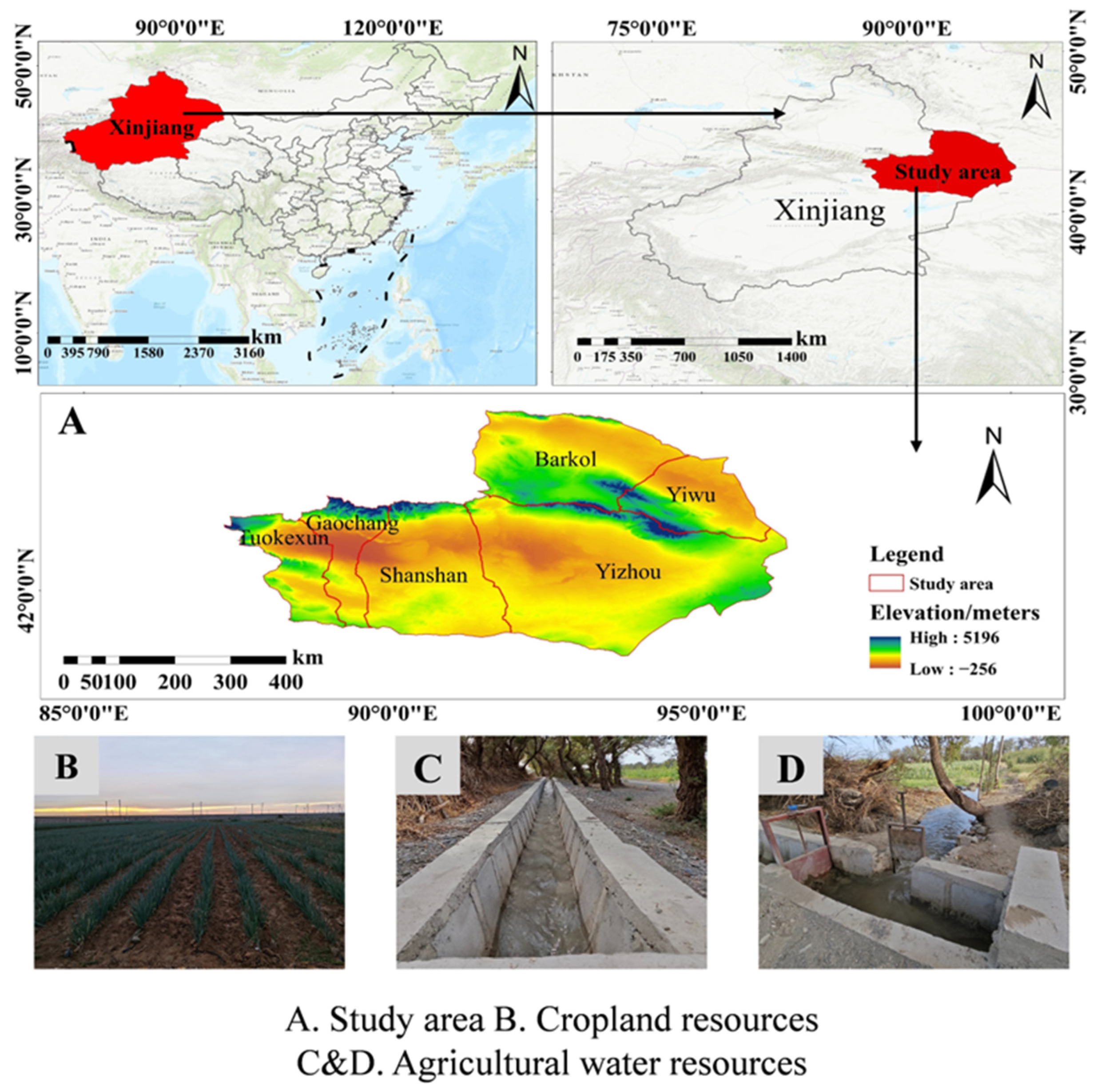
2.1. Overview of the Study Area

The Turpan–Hami Basin is located in eastern Xinjiang (87°16′–96°23′ E, 40°52′–45°05′ N), covering an area of approximately 210,000 km², which accounts for 12.6% of Xinjiang’s total land area (Figure 1). The basin encompasses six administrative divisions: Gaochang District, Shanshan County, Tuokexun County, Yizhou District, Barkol Kazakh Autonomous County, and Yiwu County. Characterized by hot, arid summers with extremely low precipitation (average annual rainfall of 47.5 mm) and strong evaporation (average annual evaporation exceeding 2000 mm), the region has an average annual temperature ranging from approximately 10.00 °C to 14.50 °C, with high temperatures peaking at up to 48.7 °C during the summer months. The region suffers from severe water scarcity, sparse vegetation, extensive land desertification, and a highly fragile ecosystem [40,41].

2.2. Data

2.2.1. Indicator System

Drawing on previous relevant studies [42,43,44] and taking into account the specific conditions of the Turpan–Hami Basin, an indicator system for evaluating the efficiency of cultivated land and agricultural water use was constructed based on panel data from statistical yearbooks, including cropping systems, capital input, labor input, resource endowment, and means of production, along with scientific validity (

Table 1. Indicator system for farmland and agricultural water resource efficiency evaluation.

Indicator Category	Data Types	Cultivated Land Indicators	Agricultural Water Resource Indicators
Input Indicators	Cropping System	Crop sown area, mu	Effective irrigated area, mu
	Capital Input	Total agricultural machinery power, kW	Total fixed asset investment, 10,000 CNY
	Labor Input	Employment in primary industry, persons	Employment in primary industry, persons
	Resource Endowment	Pesticide usage, kg	Total agricultural water use, 10,000 m3
	Means of Production	Plastic film coverage area, mu	Total grain production, tons
		Chemical fertilizer application, tons	Chemical fertilizer application, tons
Output Indicators		Gross agricultural output value, 10,000 CNY	Gross agricultural output value, 10,000 CNY

). The input indicators included resource inputs such as cultivated land, capital, machinery, labor, and water resources, while the output indicator focused on the total agricultural output value.

2.2.2. Data Sources

Based on the principle of data availability, this study utilized data from the Turpan–Hami Basin spanning 2000–2023. The primary sources include the Turpan Statistical Yearbook, Hami Statistical Yearbook, Statistical Materials of Hami Region during the 10th Five-Year Plan, Statistical Materials of Hami Region during the 11th Five-Year Plan, and the Water Resources Bulletin. Missing data were supplemented using the linear interpolation method to ensure continuity and reliability of the dataset.

2.3. Methods

2.3.1. Super-Efficiency SBM-DEA

In this study, a Super-efficiency SBM-DEA model was used to measure the efficiency of cropland resources and agricultural water use. This model was chosen due to its ability to incorporate undesirable outputs, handle slack variables directly, and enable ranking among efficient units, offering more accurate and realistic efficiency assessments in agricultural contexts. Tone [45] constructed a new SBM-DEA model that included non-expected outputs to make the assessment more realistic. $X$ is the input, assuming a total of m indicators, and $Y^g$ and $Y^b$ are the desired and undesired outputs, assuming a total of $S^1$ and $S^2$ indicators, respectively. If both the input and output indicators are greater than zero, the SBM-DEA, which contains the undesired output, takes the following form:

$${\theta }^{\ast }=\mathrm{m}\mathrm{i}\mathrm{n}{\displaystyle \frac{1-\frac{1}{m}\sum _{i=1}^m\frac{s_i^{-}}{x_{i0}}}{1+\frac{1}{r_1+r_2}\left(\sum _{q=1}^{r_1}\frac{s_q^g}{y_{q0}^g}+\sum _{t=1}^{r_2}\frac{s_t^b}{y_{t0}^b}\right)}},s.t.\left\{\begin{array}{l}X\gamma +s^{-}=x_0\\ Y^g\gamma -s^g=y_0^g\\ Y^b\gamma +s^b=y_0^b\\ \gamma \ge 0,s^{-}\ge 0,s^g\ge 0,s^b\ge 0\end{array}\right.$$

(1)

In Equation (1), ${\theta }^{\ast }$ represents the efficiency value, and $\gamma$ denotes the coefficient. $s^{-}$, $s^g$, and $s^b$ represent the slack variables for the input, desirable output, and undesirable output, respectively. When the water use efficiency is high (${\theta }^{\ast }$ = 1), $s^{-}$ = $s^g$ = $s^b$ = 0, indicating that the decision-making unit (DMU) has achieved DEA efficiency; when the water use efficiency is suboptimal (0 < ${\theta }^{\ast }$ < 1), the inputs and outputs can be adjusted to optimize efficiency.

Since the efficiency value ${\theta }^{\ast }$ ranges between 0 and 1, multiple DMUs may exhibit efficiency values equal to 1, resulting in ranking inefficiency among the DMUs. To address this limitation, Tone [46] proposed a super-efficiency SBM model, formulated as follows:

$${\rho }^{\ast }=\mathrm{m}\mathrm{i}\mathrm{n}{\displaystyle \frac{\frac{1}{m}\sum _{i=1}^m\frac{{\overline{x}}_i}{x_{i0}}}{\frac{1}{r_1+r_2}\left(\sum _{q=1}^{r_1}\frac{{\overline{y}}_q^s}{y_{q0}^s}+\sum _{t=1}^{r_2}\frac{{\overline{y}}_r^b}{y_{i0}^s}\right)}},s.t.\left\{\begin{array}{l}\overline{x}\ge \sum _{j=1,\ne k}^n{x}_j{\gamma }_j\\ {\overline{y}}^g\le \sum _{j=1,\ne k}^n{y}_j^g{\gamma }_j\\ {\overline{y}}^b\ge \sum _{j=1,\ne k}^n{y}_j^b{\gamma }_j\\ \overline{x}\ge x_0,{\overline{y}}^g\le y_0^g,{\overline{y}}^b\ge y_0^b,{\overline{y}}^g\ge 0,\gamma \ge 0\end{array}\right.$$

(2)

The functional value of ρ* is no longer confined to the [0, 1] range, thereby enabling effective ranking of water use efficiency across different units. Since these efficiency scores are relative rather than absolute measures, they are unitless and dimensionless, reflecting the comparative performance of each DMU in relation to the efficiency frontier.

2.3.2. Coupling Coordination Degree Model

The concept of coupling originates from physics, referring to the degree of mutual dependence between two or more entities, and has since been introduced into research fields such as geography, sociology, and economics [47]. The coupling degree model can be applied to explore coupling coordination relationships among systems such as regional economies [48], ecological environments [49], tourism industries [50], and ecological services [51]. This study focuses on the relationship between cultivated land and agricultural water resources within the agricultural system. The calculation formula for the coupling degree is as follows:

$$C=\sqrt{{\displaystyle \frac{U_1{\times U}_2}{{\left(\frac{U_1+U_2}{2}\right)}^2}}}$$

(3)

$U_1$ and $U_2$ represent the efficiency of cultivated land resources and agricultural water resource utilization, respectively. C denotes the coupling degree, with a range of [0, 1]. A higher C value indicates stronger interaction between the two systems.

$$T=\alpha U_1+\beta U_2$$

(4)

T is the comprehensive coordination index. $\alpha$ and $\beta$ are undetermined coefficients satisfying $\alpha +\beta =1$. To ensure equal status between the cultivated land and agricultural water resource systems in statistical measurement, this study assigns $\alpha =\beta =0.5$.

$$D=\sqrt{C\times T}$$

(5)

D represents the CCD, ranging from [0, 1]. A higher D value signifies better coordination between the systems.

Based on the current status of cultivated land and agricultural water resources in the Turpan–Hami Basin and studies by Zhu Lijuan et al. [4], the classification criteria for CCD levels are established as shown in

Table 2. Classification criteria for coupling coordination degree.

CCD	Classification Criteria
0 < D ≤ 0.2	Severe Imbalance
0.2 < D ≤ 0.4	Mild Imbalance
0.4 < D ≤ 0.6	Moderate Coordination
0.6 < D ≤ 0.8	Good Coordination
0.8 < D ≤ 1	High-quality Coordination

.

2.3.3. Kernel Density Estimation Model

Kernel density estimation (KDE) is a non-parametric method that derives continuous density functions from the data to characterize periodic and dynamic patterns of variables [52]. In this study, KDE is employed to analyze the periodic distribution characteristics and temporal evolution of the CCD between cultivated land and agricultural water resources utilization efficiency in the Turpan–Hami Basin. While traditional KDE can reveal the distribution morphology of variables, it fails to capture specific changes in a region over time. In contrast, spatial KDE estimates the probability density function of state transitions in stochastic processes, enabling precise identification of dynamic patterns through three-dimensional plots and density contour maps. This approach facilitates the exploration of regional trends over time. For the stochastic kernel estimation, the Gaussian kernel function is adopted, expressed as:

$$g\left(y|x\right)={\displaystyle \frac{f\left(x,y\right)}{f\left(x\right)}}$$

(6)

In this equation, $f\left(x\right)$ denotes the marginal kernel density function of $x$, and $f\left(x,y\right)$ represents the joint kernel density function of $x$ and $y,$ which is expressed as:

$$f\left(x,y\right)={\displaystyle \frac{1}{N{h}_x{h}_y}}{\sum }_{i=1}^N{K}_x\left({\displaystyle \frac{X_i-x}{h_x}}\right)K_y\left({\displaystyle \frac{Y_i-x}{h_y}}\right)$$

(7)

2.3.4. Dagum Gini Coefficient Decomposition Method

The Dagum Gini coefficient decomposition is a classical approach for examining spatial differentiation sources. Its core idea involves decomposing the overall Gini coefficient into contributions from intra-regional disparities, inter-regional disparities, and transvariation density by grouping subpopulations and analyzing sample distributions, effectively addressing cross-sample overlap issues [22]. The specific calculation steps are as follows:

(1) Following Dagum’s subgroup decomposition method [53], the overall Gini coefficient for the CCD between cultivated land and agricultural water resources in the Turpan–Hami Basin is defined as shown in Equation (8):

$$G={\sum }_{j=1}^k{\sum }_{h=1}^k{\sum }_{i=1}^{n_j}{\sum }_{r=1}^{n_h}{\displaystyle \frac{\left|y_{ji}-y_{hr}\right|}{2n^2\overline{y}}}$$

(8)

(2) Measurement of Intra- and Inter-Regional Gini Coefficients. Prior to decomposition, the mean coupling coordination degrees (CCDs) of counties/districts are ranked as: $Ya\le \cdots \le Yd\le \cdots \le Yk$. Based on this ranking, the intra-regional Gini coefficient $Gjj$ for region $j$ and the inter-regional Gini coefficient Gjh between regions $j$ and $h$ are calculated using Equations (9) and (10):

$$G_{jj}={\displaystyle \frac{\frac{1}{2{\overline{Y}}_j}{\Sigma }_{i=1}^{n_j}{\Sigma }_{r=1}^{n_j}\left|y_{ji}-y_{jr}\right|}{n_j^2}}$$

(9)

$$G_{jh}={\displaystyle \frac{\sum _{i=1}^{n_j}\sum _{r=1}^{n_h}\left|y_{ji}-y_{hr}\right|}{n_j{n}_h\left(\overline{Y_j}+\overline{Y_h}\right)}}$$

(10)

(3) Let $p_j=nj/Y$,$sj=njYj/nY$, where $j=\mathrm{1,2},3,\dots ,k$; $D_{jh}$ denotes the interaction intensity of CCDs between regions $j$ and $h$, $d_{jh}$ represents the difference in CCDs between regions, defined as the mathematical expectation of $y_{ji}-y_{hr}>0$, and $p_{jh}$ represents the mathematical expectation of $y_{ji}-y_{hr}<0$. These are calculated using Equations (11)–(13):

$$D_{jh}=\left(d_{jh}-p_{jh}\right)/\left(d_{jh}+p_{jh}\right)$$

(11)

$$d_{jh}={\int }_0^{\mathrm{\infty }}d{F}_J\left(y\right){\int }_0^y\left(y-x\right)d{F}_h\left(x\right)$$

(12)

$$p_{jh}={\int }_0^{\mathrm{\infty }}d{F}_h\left(y\right){\int }_0^y\left(y-x\right)d{F}_j\left(y\right)$$

(13)

(4) Dagum decomposes the Gini coefficient (G) into three components [54]: intra-regional disparity contribution (G_w), inter-regional net disparity contribution (G_b), and transvariation density (G_t), satisfying the relationship $G=G_{\mathrm{w}}+G_{\mathrm{b}}+G_{\mathrm{t}}$. Here, G_t quantifies the impact of cross-regional overlapping terms on the overall disparity. The calculations for G_w, G_b, and G_t are shown in Equation (14):

$$G_{\mathrm{w}}={\sum }_{j=1}^k{G}_{jj}{p}_j{s}_j$$

(14)

$$G_{\mathrm{b}}={\sum }_{j=2}^k{\sum }_{h=1}^{j-1}{G}_{jh}\left(p_j{s}_h+p_h{s}_j\right)D_{jh}$$

(15)

$$G_{\mathrm{t}}={\sum }_{j=2}^k{\sum }_{h=1}^{j-1}{G}_{jh}\left(p_j{s}_h+p_h{s}_j\right)\left(1-D_{jh}\right)$$

(16)

2.3.5. Moran’s I

Moran’s I is one of the most critical metrics for measuring and characterizing the spatial distribution patterns and interdependencies of variables, as well as their clustering tendencies. In this study, Moran’s I is employed to further analyze the spatial correlation of the CCD between cultivated land and agricultural water resources utilization efficiency in the Turpan–Hami Basin. The Moran’s I encompasses global and local spatial autocorrelation, with the formulas defined as follows:

$$Global Mora{n}^{’}s I = {\displaystyle \frac{n{\sum }_{i=1}^n{\sum }_{j=1}^n{W}_{ij}(x_i-\overline{x})(x_j-\overline{x})}{\left({\sum }_{i=1}^n{\sum }_{j=1}^n{W}_{ij}\right){\sum }_{i=1}^n{(x_i-\overline{x})}^2}}$$

(17)

$$Local Mora{n}^{’}s I = {\displaystyle \frac{n(x_i-\overline{x}){\sum }_{j=1}^n{W}_{ij}(x_j-\overline{x})}{{\sum }_{i=1}^n{(x_i-\overline{x})}^2}}$$

(18)

where $n$ denotes the number of spatial units, $xi$ and $xj$ represent the values of variable $x$ at spatial locations $i$ and $j,$ respectively, $\overline{x}$ is the mean value of $x$, and $W_{ij}$ is the spatial weight matrix. In this study, a contiguity-based spatial weight matrix is adopted, where $W_{ij}$ is assigned a value of 1 if regions $i$ and $j$ are adjacent, and 0 otherwise.

Drawing on insights from relevant high-quality research and aligning with the innovative aspects of this study, the main analytical framework is illustrated in Figure 2.

3. Results

3.1. Analysis of Cultivated Land and Agricultural Water Resource Utilization Efficiency

To explore the spatiotemporal characteristics of cultivated land and agricultural water resource utilization efficiency in the Turpan–Hami Basin, a non-radial super-efficiency SBM model with variable returns to scale (VRS) in DEARUN 3.2.0 was applied. The results are detailed in

Table 3. Cultivated land and agricultural water use efficiency values in Turpan–Hami Basin (unitless scores).

Year	Farmland Resources						Agricultural Water Resource Utilization Efficiency
	Gaochang	Shanshan	Tuokexun	Yizhou	Barkol	Yiwu	Gaochang	Shanshan	Tuokexun	Yizhou	Barkol	Yiwu
2000	0.122	0.072	0.069	0.115	2.830	0.142	0.205	0.102	0.377	0.208	1.050	1.330
2001	0.179	0.108	0.137	0.114	0.803	0.151	0.286	0.166	0.412	0.165	0.745	0.448
2002	0.158	0.152	0.221	0.125	0.706	0.168	0.427	0.188	1.013	0.163	1.016	0.357
2003	0.196	0.143	0.263	0.144	0.714	0.243	0.529	0.201	0.543	0.179	1.040	0.841
2004	0.176	0.179	0.162	0.157	1.011	0.279	0.536	0.241	0.231	0.234	1.024	1.010
2005	0.204	0.177	0.268	0.164	0.265	0.322	1.052	0.238	0.355	0.274	1.029	1.024
2006	0.236	0.252	0.237	0.175	0.219	0.382	1.026	0.251	0.343	0.226	0.673	0.547
2007	0.269	0.326	0.340	0.188	0.276	0.526	1.024	0.302	0.399	0.234	0.702	0.775
2008	0.276	0.343	0.281	0.205	0.397	1.007	0.525	0.310	0.383	0.228	1.049	1.043
2009	0.282	0.369	0.397	0.234	0.392	0.524	0.407	0.346	0.323	0.235	0.499	0.661
2010	0.300	0.370	0.369	0.256	0.461	0.627	0.394	0.423	0.344	0.256	0.459	0.632
2011	0.342	0.374	0.315	0.300	0.466	1.021	0.397	0.384	0.272	0.307	0.480	1.015
2012	0.444	0.437	0.398	0.329	0.487	0.626	0.505	1.011	0.275	0.340	0.504	0.528
2013	0.588	0.525	0.382	0.363	0.565	0.701	0.754	0.507	0.306	0.298	0.494	0.649
2014	0.612	0.442	0.390	0.332	0.565	0.701	1.011	0.443	0.335	0.297	0.511	0.538
2015	0.659	0.495	0.427	0.349	1.020	0.841	1.014	0.563	0.344	0.312	0.583	0.849
2016	0.689	0.541	0.475	0.371	1.022	1.025	0.561	0.528	0.368	0.346	0.853	1.109
2017	0.644	0.480	0.465	0.335	0.790	0.696	0.469	0.476	0.355	0.328	0.714	0.882
2018	0.729	0.521	0.437	0.317	0.704	0.609	0.595	0.634	0.347	0.338	0.629	0.587
2019	0.729	0.546	0.481	0.357	0.675	0.653	0.633	1.208	0.363	0.358	0.812	0.695
2020	0.765	0.832	0.595	0.428	0.736	0.868	0.870	0.978	0.450	0.422	1.048	0.837
2021	0.917	1.042	0.756	0.455	0.723	1.028	1.052	1.016	0.564	0.493	0.810	1.031
2022	1.091	1.063	1.012	0.477	1.085	0.959	1.144	0.796	1.026	0.775	1.040	1.045
2023	1.008	1.002	1.175	0.375	0.892	0.679	1.026	1.052	0.981	1.036	1.021	1.069
Mean	0.484	0.450	0.419	0.278	0.746	0.616	0.685	0.515	0.446	0.335	0.783	0.812

and Figure 3a. The analysis reveals that the overall efficiency of cultivated land utilization in the Turpan–Hami Basin remained relatively low during the study period, with an average value of 0.516, indicating significant room for improvement. The ranking of mean efficiency across counties/districts is as follows: Barkol Kazakh Autonomous County (0.746) > Yiwu County (0.616) > Gaochang District (0.484) > Shanshan County (0.450) > Tuokexun County (0.419) > Yizhou District (0.278). Although Barkol Kazakh Autonomous County ranked first, its efficiency exhibited a fluctuating trend, initially rising and then declining sharply. Notably, the cultivated land efficiency in Barkol plummeted between 2000 and 2001. This decline is primarily attributed to a dramatic increase in agricultural production costs driven by the surge in plastic film usage. Although Barkol Kazakh Autonomous County ranked first in cultivated land resource efficiency, it exhibited an overall trend of initial fluctuation upward followed by a decline. A notably sharp decrease occurred during the period from 2000 to 2001, primarily due to the rapid expansion of plastic film mulching area. Specifically, the area covered by plastic film increased dramatically from 60 mu in 2000 to 705 mu in 2001, and further to 1350 mu in 2002, representing a 21.5-fold increase. This surge in plastic film usage directly led to significant rises in agricultural production costs, including materials and labor, whereas other input indicators, such as crop sowing area and total agricultural machinery power, did not experience significant growth during the same period. Consequently, the cultivated land resource efficiency of Barkol Kazakh Autonomous County experienced a precipitous decline from 2000 to 2001. In contrast, the efficiency growth of cultivated land utilization in Turpan far exceeded that of Hami. Gaochang District, Shanshan County, and Tuokexun County achieved efficiency increases exceeding 85%, while Yizhou District’s efficiency remained below 0.5. Notably, Barkol even experienced negative growth. These findings suggest that Turpan’s practices in enhancing land-use efficiency could offer valuable insights for Hami to address its inefficiencies.

As shown in Table 3 and Figure 3b, the agricultural water resource utilization efficiency in the Turpan–Hami Basin exhibits a fluctuating upward trend, with overall efficiency values higher than those of cultivated land utilization. From 2000 to 2023, Shanshan County achieved the most significant efficiency growth at 90.3%. Specifically, the water resource utilization efficiency in Gaochang District and Yiwu County exhibits a distinct ‘W’-shaped fluctuation pattern. In Yiwu County, although the efficiency level was relatively high in 2000, it subsequently declined—a trend potentially associated with the rapid expansion of fixed asset investments. From 2000 to 2002, Yiwu County’s total fixed asset investment surged from CNY 9.58 million to CNY 86.50 million, marking a 7.95-fold increase over three years. However, this substantial capital influx failed to drive concurrent improvements in critical agricultural water efficiency indicators, such as total agricultural water consumption and effective irrigated area, revealing a disconnect between investment scale and resource productivity. Parallel to the cultivated land resource trends, Yizhou District demonstrates persistently low efficiency values with minimal growth, primarily attributable to its arid climate characterized by low annual precipitation and high evaporation rates. Agricultural water supply in this region relies heavily on limited groundwater extraction and river diversions, resulting in chronic water scarcity that directly constrains irrigation efficiency. In contrast, Barkol Kazakh Autonomous County and Tuokexun County achieved notable efficiency improvements post-2010, likely driven by the adoption of agricultural mechanization and water-saving technologies. Future strategies should prioritize scaling water-saving innovations to enhance agricultural water-use efficiency and mitigate water supply–demand imbalances.

3.2. Coupling Coordination Degree Analysis of Cultivated Land and Agricultural Water Resource Utilization Efficiency

3.2.1. Temporal Evolution Characteristics of Coupling Coordination Degree

The temporal variation of the CCD (D-value) between cultivated land resources and agricultural water resource utilization efficiency in the Turpan–Hami Basin is shown in Figure 4. During the study period, the mean D-values across districts/counties ranked as follows: Barkol Kazakh Autonomous County (0.587) > Yiwu County (0.563) > Gaochang District (0.494) > Shanshan County (0.437) > Tuokexun County (0.417) > Yizhou District (0.342). The regional averages clustered around 0.4, indicating no significant hierarchical imbalance. The temporal evolution exhibited a phased improvement trend with distinct spatial heterogeneity, divided into three stages: firstly, 2000–2010 marked a low-efficiency fluctuation period, characterized by D-values below 0.5 in most districts/counties, dominated by moderate imbalance, with Gaochang District and Yizhou District persistently stagnating at low D-values (0.2–0.3) due to inadequate mechanization levels; secondly, 2010–2020 represented a gradual ascending phase, during which D-values achieved an average annual growth rate of 5.2% driven by water-saving technological advancements and policy interventions, with Gaochang District and Yiwu County becoming the first regions to reach moderate coordination or higher levels; finally, 2020–2023 emerged as a high-efficiency synergy phase, where multiple districts/counties surpassed the D-value threshold of 0.7, including Gaochang District and Tuokexun County, which achieved high-quality coordination.

The Turpan–Hami Basin exhibited significant spatial heterogeneity, demonstrating a “dual-core driving–marginal lagging” pattern. Gaochang District and Yiwu County formed the “dual-core drivers”, while Yizhou District remained in sub-moderate coordination, representing a peripheral lagging zone. Barkol Kazakh Autonomous County experienced drastic early-stage fluctuations, attributable to abrupt increases in plastic mulch coverage, intensified water resource pressures, and disconnects between policies and technologies. Tuokexun County and Yizhou District displayed smoother curves with sustained higher coordination levels, reflecting stable inter-system harmonization. In contrast, Yiwu County showed greater D-value volatility, indicating unstable coordination between systems.

Overall, the coupling coordination degrees of the six counties exhibited an upward trend with notable spatial differentiation. Based on the observed trends, preliminary projections suggest that if current improvements in water-use efficiency continue, most counties in the Turpan–Hami region could reach a “good coordination” level by 2035. However, in scenarios where efficiency stagnates, CCD growth may slow or even decline. These scenario-based insights, although exploratory, highlight the importance of proactive water and land management strategies in shaping future coordination outcomes.

To further examine the temporal evolution of the CCD between cultivated land and agricultural water resources, a linear regression analysis was conducted for each county based on the CCD values presented in Figure 4, with results summarized in

Table 4. Linear regression analysis.

County/District	Regression Equation	R2	Trend Interpretation
Gaochang	$y$ = −35.09098 + $0.01769x$	0.81949	Moderate-to-strong upward trend
Shanshan	$y$= −46.38997 + $0.02328x$	0.93279	Strong and steady upward trend
Tuokexun	$y$ = −23.96546 + $0.01212x$	0.54497	Moderate upward trend
Yizhou	$y$= −25.57487 + $0.01288x$	0.91584	Significant upward trend
Barkol	$y$= 0.5828 + $0.0003x$	0.0004	No meaningful linear trend
Yiwu	$y$= −23.78798 + $0.01211x$	0.54231	Moderate upward trend

. The regression equations and coefficients of determination (R²) reflect significant regional differences in the coordination process. Shanshan County, Yizhou District, and Gaochang District showed strong linear relationships, with R² values of 0.93279, 0.91584, and 0.81949, respectively, indicating a clear upward trend in CCD over time and a strong capacity for coordinated land–water development. Tuokexun and Yiwu Counties exhibited weaker fits (R² = 0.54497 and 0.54231), suggesting general improvement but with more pronounced fluctuations. In contrast, Barkol County’s regression showed almost no explanatory power (R² = 0.0004), and the slope was close to zero, indicating high variability and a lack of a clear linear trend during the study period. To further explore this issue, the CCD of Barkol County was analyzed in two phases: 2000–2011 and 2012–2023. As shown in Figure 5, the first phase exhibited a negative regression slope and an R² of 0.602, reflecting a declining trend with significant fluctuations. This decline coincided with several extreme drought events in Xin-jiang (e.g., 2001 and 2006), which, along with high temperatures and reduced precipitation, likely limited water supply and agricultural productivity—contributing to the weakening of coordination between land and water resources [55]. In the second phase (2012–2023), the slope turned positive and the R² value increased, suggesting a slow recovery in coordination, potentially driven by the promotion of water-saving technologies and supportive regional policies. However, fluctuations persisted; for example, the severe drought in 2013 continued to disrupt progress, highlighting the ongoing vulnerability of land–water systems to extreme climatic events, even amid gradual improvement.

Building on the temporal analysis, kernel density plots were employed to reveal the dynamic evolution of the coupling coordination between cultivated land and agricultural water resources utilization efficiency in the Turpan–Hami Basin. As shown in Figure 6: (1) In terms of distribution position, the overall kernel density curves exhibit bell-shaped fluctuations, particularly in low coupling coordination intervals (D < 0.3). The primary peak shifts rightward over time, indicating gradual improvements in coordination levels, consistent with earlier findings. Specifically, the curves display a multi-layered oscillating trend (“left-right-left-right”), with minor peaks emerging in low coordination regions (near D = 0). The height of these peaks reflects the density or concentration of data points in specific intervals. Significant fluctuations in low coordination regions (D < 0.3) suggest substantial inter-system disparities during early stages, likely attributable to external factors or developmental instability. Post-2010, the dominant peak progressively shifts toward higher coordination values (D > 0.5), signaling enhanced systemic synergy and clustering of high-coordination data points. (2) In terms of distribution pattern, regional disparities in coordination levels show a narrowing trend. The height of the primary peak undergoes a “rise-fall-rise” evolution, while its width gradually contracts. The kernel density curves transition from flat and wide (indicating pronounced regional disparities) to sharp and narrow (reflecting reduced absolute differences), suggesting improved coordination homogeneity across the Turpan–Hami Basin over the study period. (3) In terms of distribution extensibility, the density curves exhibit rightward tailing, implying an increase in the number of counties/districts with higher coordination degrees (D ≥ 0.6). A distinct peak persists near D = 0, followed by a gradual density decline and a minor tail in the 0.7–0.8 range. This pattern illustrates a gradual shift from low coordination (D ≈ 0) to moderate-high coordination (D ≈ 0.6) intervals, demonstrating the system’s incremental progression toward higher coordination. While long-term coordination remains predominantly low-to-moderate, the trend toward higher values underscores maturing coordination mechanisms and enhanced collaborative capacity, albeit with residual fluctuations and disparities in specific periods or domains. (4) In terms of polarization trend, despite persistent fluctuations, polarization becomes increasingly pronounced. Early years feature prominent peaks in low-coordination regions (D < 0.3), indicating weak inter-system collaboration. Post-2010, the number of peaks transitions from bimodal to unimodal, and the dominant peak shifts rightward, concentrating near D = 0.6. This evolution highlights intensified polarization toward moderate-high coordination levels, reflecting systemic maturation and targeted efficiency enhancements.

3.2.2. Spatial Evolution Characteristics of Coupling Coordination Degree

To investigate the spatial evolution of the CCD between cultivated land and agricultural water resources utilization efficiency in the Turpan–Hami Basin, ArcGIS 10.4 (ESRI, NY Str., Redlands, CA, USA) software was used to visualize the CCD (D-value) at four key time points: 2005, 2011, 2017, and 2023 (Figure 7). Combined with the efficiency values of cultivated land and agricultural water resources from 2000 to 2023 (Table 2), the lag types of coordination in each county/district were further analyzed. Overall, areas with good coordination in the Turpan–Hami Basin evolved from scattered points to clustered patterns, expanding from west to northeast, forming a “dual-core driving–marginal lagging” spatial structure, and progressing toward higher coordination levels, consistent with the conclusions above. Specifically, in 2005, Gaochang District, Barkol Kazakh Autonomous County, and Yiwu County exhibited moderate coordination, while other counties/districts were in mild imbalance. By 2011, Yiwu County transitioned to good coordination, and Shanshan County improved to general coordination. In 2017, all three counties/districts in Turpan City achieved moderate coordination, while Yizhou District in Hami City remained in mild imbalance, though Barkol Kazakh Autonomous County advanced to good coordination. By 2023, the number of areas with good coordination increased to five, with only Yizhou District reaching primary coordination.

Based on the evolution of coordination types in counties/districts, three development pathways emerged: leapfrog, growth, and stable types. During the study period, Turpan City exhibited balanced and steady improvements in coupling coordination, transitioning from mild imbalance to good coordination. Despite being an ecologically fragile and water-scarce region, its coordination improved significantly in recent years due to ecological restoration and enhanced water-use efficiency, representing a stable development pathway. Yizhou District in Hami City followed a growth-type pathway, shifting from mild imbalance to primary coordination. However, its overall coordination remained low, with insignificant upward trends and a notable lag in water resource efficiency. Barkol Kazakh Autonomous County and Yiwu County followed a leapfrog-type pathway, advancing from intermediate to high-quality coordination. Their late-stage coordination peaked but displayed fluctuations in the efficiency of cultivated land and water resource utilization.

3.3. Analysis of Regional Differences in Coupling Coordination Degree

To further investigate the sources and evolution of spatial differentiation in the CCD between cultivated land and agricultural water resource utilization efficiency in the Turpan–Hami Basin, the study area was geographically divided into two subregions. The Dagum Gini coefficient decomposition method was employed to quantify the overall Gini coefficient (G), intra-regional disparities, inter-regional disparities, and the intensity of transvariation (

Table 5. Dagum Gini Coefficient.

Year	Gini Coefficient	Intra-Regional Disparity		Inter-Regional Disparity	Contribution Rate (%)
		Turpan	Hami	Turpan–Hami	Intra-Regional	Inter-Regional	Hypervariation Density
2000	0.374	0.152	0.298	0.488	34.78	65.05	0.17
2001	0.213	0.092	0.243	0.246	42.37	41.16	16.46
2002	0.221	0.149	0.253	0.238	46.15	14.22	39.63
2003	0.200	0.113	0.213	0.229	42.50	33.10	24.41
2004	0.213	0.072	0.204	0.273	36.05	56.25	7.70
2005	0.137	0.112	0.123	0.156	43.05	30.99	25.95
2006	0.114	0.096	0.111	0.123	45.68	1.16	53.16
2007	0.120	0.071	0.144	0.132	44.83	3.44	51.72
2008	0.169	0.024	0.185	0.222	34.36	43.26	22.38
2009	0.092	0.005	0.120	0.118	35.51	24.07	40.42
2010	0.092	0.018	0.116	0.115	37.82	26.65	35.53
2011	0.135	0.036	0.155	0.165	38.64	52.16	9.20
2012	0.085	0.094	0.068	0.089	47.61	5.92	46.48
2013	0.090	0.087	0.092	0.091	49.45	0.19	50.35
2014	0.103	0.103	0.084	0.113	45.27	10.81	43.92
2015	0.113	0.097	0.111	0.121	46.33	11.91	41.76
2016	0.126	0.051	0.125	0.160	36.35	39.98	23.67
2017	0.100	0.039	0.101	0.127	36.27	33.82	29.91
2018	0.079	0.066	0.087	0.082	48.12	5.32	46.56
2019	0.089	0.082	0.088	0.092	47.94	12.34	39.72
2020	0.079	0.067	0.085	0.083	47.80	8.20	44.00
2021	0.080	0.054	0.093	0.088	45.07	29.59	25.34
2022	0.049	0.023	0.064	0.056	43.39	39.69	16.93
2023	0.046	0.006	0.057	0.062	32.53	67.47	0.00
Mean	0.130	0.071	0.134	0.153	42.00	27.36	30.64

, Figure 8).

As shown in Table 4, the overall Gini coefficient (G-value) of CCD in the Turpan–Hami Basin exhibited a significant downward trend from 0.374 in 2000 to 0.046 in 2023, with an average annual decline of 8.7%, indicating a narrowing trend in regional disparities. The process can be categorized into three phases: 2000–2007 saw a sharp reduction in the G-value, potentially linked to the adoption of water-saving technologies and the establishment of interregional collaboration mechanisms. Next, 2007–2016 was characterized by pronounced fluctuations in the G-value, with an average annual decline of 5%, primarily attributable to uneven resource allocation and insufficient policy coverage. Then, 2016–2023 entered a low-disparity stabilization phase, during which the G-value approached zero, and the contribution of hypervariability density dropped to 0%, signifying a balanced and coordinated development pattern across all districts/counties.

Regarding intra-regional differences (Figure 8a), the Gini coefficient in Turpan decreased from 0.152 in 2000 to 0.006 in 2023, with an annual decline of 9.2%, reflecting rapid internal homogenization of resource utilization efficiency. In contrast, Hami consistently exhibited higher intra-regional disparities than Turpan, likely due to uneven distribution of irrigation technologies and facilities, though improvements became evident post-2015.

For inter-regional differences, the disparities between Turpan and Hami showed a fluctuating downward trend over time, peaking in 2000 due to severe resource coordination imbalances. This was attributed to uneven regional development during the rapid economic growth of the “12th Five-Year Plan” period (2011–2015), driven by variations in resource endowments, industrial structures, fiscal policies, and rural development levels. Subsequent policies, such as the 13th Five-Year Plan for High-Quality Development in Xinjiang [56], the Arid Region Ecological Protection and Restoration Action Plan [57], and the implementation of large-scale water-saving agricultural demonstration zones, promoting high-quality regional development and ecological protection, mitigated these disparities.

In terms of contributions to regional differences (Figure 8b), intra-regional disparities (G_w) contributed the most (42.0%) with minimal fluctuations, followed by transvariation density (G_t) at 30.64%, which first rose and then declined. Inter-regional disparities (G_b) contributed the least (27.36%) but exhibited the largest fluctuations. These results indicate that intra-regional differences and transvariation density from cross-regional overlaps are the primary sources of spatial differentiation in coordination development.

3.4. Spatial Aggregation Characteristics of Coupling Coordination Degree

To explore the spatial aggregation characteristics of the CCD between cultivated land and agricultural water resources in the Turpan–Hami Basin, the global Moran’s I was calculated using an inverse distance spatial weight matrix in ArcGIS. As shown in

Table 6. Global Moran index.

Year	Moran’s I	Z	p-Value
2000	0.13	1.003	0.158
2004	0.061	0.793	0.214
2013	−0.562	−1.1	0.136
2023	−0.054	0.443	0.329

, from 2000 to 2023 (excluding 2000), Moran’s I values were negative, fluctuating between −0.56 and −0.32, showing an overall “first decline then rise” trend. This indicates that the spatial distribution pattern of the CCD in the Turpan–Hami Basin tends to be random with weak spatial aggregation. Specifically, it can be divided into three periods: Positive Correlation Period (2000–2004): In 2000, Moran’s I = 0.13 (p = 0.158), which did not pass the significance test but reflected weak spatial clustering of efficiency values in the early stage. Negative Correlation Dominance Period (2005–2020): In 2013, Moran’s I reached its lowest value of −0.56 (p = 0.136), indicating expanded differences in resource utilization efficiency and enhanced spatial heterogeneity. Recovery Period (2021–2023): By 2023, Moran’s I rose to −0.054 (p = 0.329).

Due to the limited number of spatial units (six counties), the global Moran’s I values from 2000 to 2023 did not pass the significance test (p > 0.1). This is consistent with expectations, as spatial autocorrelation results are often sensitive to small sample sizes. Moreover, the weak and insignificant spatial aggregation reflects the spatially fragmented nature of CCD distribution in the region, shaped by uneven development and heterogeneous land–water resource conditions.

To further investigate the spatial clustering patterns of the CCD in the Turpan–Hami Basin from 2000 to 2023, the local Moran’s I index was employed. The analysis revealed a significant “core–periphery” polarization pattern, with clustering types undergoing phased changes in response to policy shifts and environmental constraints. As shown in

Table 7. Local Moran index.

Types	2000	2010	2016	2020	2023
High-High (HH) Cluster	Barkol	Shanshan			Gaochang
High-Low (HL) Cluster					Shanshan Barkol
Low-High (LH) Cluster	Yizhou	Yizhou	Yizhou	Yizhou	Yizhou
Low-Low (LL) Cluster	Shanshan		Gaochang Shanshan		Yiwu

, Shanshan County and Gaochang District were classified as high-high clustering types in 2010 and 2023, indicating their high internal coordination levels and synchronized efficiency improvements with adjacent Tuokexun County. These counties should continue to enhance the sharing of water-saving and irrigation technologies to drive synergistic development in surrounding areas. Barkol Kazakh Autonomous County and Shanshan County exhibited high-low clustering characteristics in 2023, reflecting their high internal coordination but neighboring Yizhou District’s persistently low efficiency (D < 0.5). Cross-regional technology transfer and infrastructure co-construction should be prioritized to avoid “island effects” and actively guide the orderly transfer of local resources to neighboring low-coordination areas. Yizhou District remained a low-high clustering type over the long term, indicating its low coordination level despite higher efficiency in adjacent counties. This area should leverage resource spillovers from neighboring regions to address bottlenecks such as aging irrigation facilities. Yiwu County exhibited low-low clustering in 2023, constrained by resource underutilization and geographic isolation, with neighboring Yizhou District also showing low coordination. Policy incentives and ecological compensation mechanisms are essential to break the cycle of low coordination. Overall, approximately 60% of districts/counties in the Turpan–Hami Basin failed to pass significance tests (p > 0.1), demonstrating weak spatial aggregation effects and fragmented synergy patterns, which reflect persistent challenges in technology diffusion and policy coverage [58,59].

4. Discussion

4.1. Spatiotemporal Differentiation Characteristics of Coupling Coordination Degree

This study measured the utilization efficiency of cultivated land and agricultural water resources in six counties/districts of the Turpan–Hami Basin from 2000 to 2023 based on the coupling mechanism between these resources, using a super-efficiency non-radial SBM-DEA model. The spatiotemporal distribution characteristics of their CCD were analyzed. The integration of the super-efficiency SBM-DEA model with the traditional coupling coordination model achieved scientific optimization of comprehensive development indicators. First, the super-efficiency SBM-DEA model, by objectively assigning weights based on DEA, avoids biases from subjective weighting methods like entropy weighting and dynamically reflects the actual marginal contributions of input-output indicators. Second, the model corrects raw data efficiency using slack variables, with the super-efficiency design breaking the 1.0 efficiency limit. Combined with global frontier construction, it enhances the comparability of intertemporal technical efficiency [46]. This method significantly improves the accuracy of resource coupling coordination evaluation in arid regions through an “efficiency optimization-indicator reconstruction-system coordination” integration pathway, particularly suitable for identifying typical issues like “high input, low efficiency, weak coordination” in Turpan–Hami agriculture, providing robust technical support for precise water-saving technologies and differentiated regulatory policies.

The results show that the mean CCD in the Turpan–Hami Basin increased from 0.32 (moderate imbalance) to 0.68 (good coordination) during the study period, with an annual growth rate of 4.6%, exhibiting a three-stage transition: “low-efficiency fluctuation–steady improvement–high-quality synergy”. This aligns with findings from typical arid regions such as Xinjiang [3,60], the lower Yellow River Basin [36], and the Hexi Corridor [61], confirming the positive role of technological progress and policy interventions in promoting efficient resource synergy. However, compared to the Huai River Basin [62] (annual growth rate ≈ 8.9%), Turpan–Hami’s slower growth reflects ecological fragility’s constraints on regional coordination.

Second, the CCD exhibited a “dual-core driving–marginal lagging” spatial pattern. Gaochang District and Yiwu County formed high-efficiency “dual cores”, with coordination degrees reaching 0.71 and 0.65 in 2023, while Yizhou District remained in low-coordination fluctuation due to imbalanced resource allocation and delayed adoption of water-saving technologies. Three-dimensional kernel density analysis further revealed that high-coordination areas (D ≥ 0.6) gradually expanded toward peripheral regions post-2015 but failed to form contiguous synergy, highlighting spatially uneven technology diffusion. Therefore, future efforts should prioritize inter-regional technology exchange and policy coordination to optimize resource allocation and advance arid agricultural resource coupling systems toward higher-level, broader coordination.

4.2. Analysis of Regional Spatial Differences

The Dagum Gini coefficient decomposition revealed that intra-regional disparity (G_w) contributed the most to the total disparity (mean contribution of 42.0%), followed by supervariability density (G_t, 30.64%) and inter-regional disparity (G_b, 27.36%). This result aligns with findings from the Chengdu–Chongqing urban agglomeration [63] (G_t contribution: 27.12%), but the significantly higher inter-regional contribution reflects intensified cross-district competition for resources in the Turpan–Hami Basin. For instance, Barkol Kazakh Autonomous County exhibited an artificially inflated coordination degree (D = 0.93) during 2000–2002 due to a sharp increase in plastic mulch coverage, yet its technological pathway failed to diffuse to neighboring areas, exacerbating inter-regional disparities.

Global Moran’s I analysis indicated weak overall spatial correlation of coordination degrees (Moran’s I = −0.56 to −0.32) but significant local clustering. Shanshan County and Gaochang District displayed high-high clustering (HH type, p < 0.1) in 2016 and 2023, while Yizhou District persistently exhibited low-high clustering (LH type), mirroring the polarization patterns observed in county-level ecological-economic system coordination in Jiangsu Province [64]. As a typical LH-type area, Yizhou District’s low coordination degree starkly contrasted with the high coordination of its neighbor, Shanshan County. This disparity suggests that highly coordinated regions may generate a “siphon effect” [65], attracting resource concentration while inhibiting resource diffusion and synergistic development in adjacent areas.

This study, guided by the concept of high-quality development, establishes a coupling coordination analysis framework between cultivated land and agricultural water resources, revealing the theoretical mechanism of their integrated optimization in arid regions. It helps address current gaps in understanding the non-linear relationships and spatial heterogeneity within resource systems. However, as the CCDM is essentially descriptive, it simplifies causal mechanisms and dynamic feedback. Future studies could incorporate causal inference approaches (e.g., econometric models) or simulation tools (e.g., system dynamics) to better capture how policy, economic, and environmental factors interact and influence land–water coordination over time. Integrating these approaches will help support more adaptive management strategies and provide stronger decision-making support for sustainable resource planning in arid regions.

5. Conclusions

This study measured the utilization efficiency of cultivated land and agricultural water resources in the Turpan–Hami Basin from 2000 to 2023, analyzing their coordinated development levels, spatiotemporal evolution patterns, and spatial aggregation effects using CCDM. Key findings include: The overall efficiency of cultivated land and agricultural water resources utilization in Turpan–Hami was relatively low, with mean values of 0.516 and 0.596, respectively, showing fluctuating upward trends and significant spatial heterogeneity. The top three efficient areas were Barkol Kazakh Autonomous County, Yiwu County, and Gaochang District. The mean CCD across regions ranked as: Barkol Kazakh Autonomous County (0.587) > Yiwu County (0.563) > Gaochang District (0.494) > Shanshan County (0.437) > Tuokexun County (0.417) > Yizhou District (0.342). The regional mean CCD increased from 0.32 (moderate imbalance) to 0.68 (good coordination), with an annual growth rate of 4.6%, exhibiting three phases: “low-efficiency fluctuation (2000–2010), steady improvement (2010–2020), high-quality synergy (2020–2023).” Regional disparities were pronounced: Gaochang District and Yiwu County formed high-efficiency “dual cores” (D = 0.75 and 0.72 in 2023), while Yizhou District (0.55) remained in low coordination due to a technological lag and resource mismatch. Three-dimensional kernel density analysis revealed post-2015 diffusion of high coordination (D ≥ 0.6) to peripheral areas without forming contiguous synergy. Dagum Gini coefficient decomposition showed that intra-regional differences (G_w) contributed 42.0%, transvariation density (G_t) 30.64%, and inter-regional differences (G_b) 27.36% to the total variation. Spatial autocorrelation analysis identified a “core-periphery” polarization pattern, with Gaochang District and Shanshan County as high-high clusters (HH type) and Yizhou District as a persistent low-high cluster (LH type).

References

1. Fan, H.; Fu, W.G. Agricultural water-soil resource matching and agricultural economic growth in China from a water footprint perspective: A case study of the Yangtze River Economic Belt. Chin. J. Agric. Resour. Reg. Plan. 2020, 41, 193–203. [Google Scholar]
2. Huang, S.; Fu, Y.; Zhang, Y.; Yang, J. Coupling coordinated development of water-energy-food-forest systems in the Yangtze River Basin. Acta Ecol. Sin. 2024, 32, 1193–1205. [Google Scholar]
3. Jiang, S.; Hu, B. Spatial evolution measurement of cultivated land and water resources in arid regions: A case study of Xinjiang. Water Resour. Dev. Res. 2023, 23, 26–32. [Google Scholar]
4. Zhu, L.; Lu, Q. Spatial correlation analysis of cultivated land and irrigation water resource utilization efficiency and their coupling coordination degree in China’s provinces. J. China Agric. Univ. 2022, 27, 297–308. [Google Scholar]
5. Chen, J.; Yu, X.; Qiu, L.; Deng, M.; Dong, R. Study on vulnerability and coordination of Water-Energy-Food system in Northwest China. Sustainability 2018, 10, 3712. [Google Scholar] [CrossRef]
6. Yang, Y.; Yang, J.; Xu, Y.; Zhao, X. Analysis of production water use changes in Xinjiang based on LMDI method. Arid Land Geogr. 2016, 39, 67–76. [Google Scholar]
7. Hu, J.; Ding, J.; Zhang, Z.; Wang, J.; Liu, J. Estimation of vegetation ecological water demand in the Turpan-Hami region over the past 30 years. Acta Ecol. Sin. 2024, 44, 8699–8715. [Google Scholar]
8. Junran, D.; Desheng, W. An Evaluation of the Impact of Ecological Compensation on the Cross-Section Efficiency Using SFA and DEA: A Case Study of Xin’an River Basin. Sustainability 2020, 12, 7966. [Google Scholar]
9. Abudureheman, A.; Wang, Y.; Rao, F. Factors influencing cotton farmers’ water resource utilization efficiency under participatory irrigation management: A case study in Awat County, Xinjiang. J. Arid Land Resour. Environ. 2018, 9, 183–189. [Google Scholar]
10. Li, M. Research on agricultural water resource utilization efficiency in China based on DEA method. Chin. J. Agric. Resour. Reg. Plan. 2017, 38, 106–114. [Google Scholar]
11. Liu, X.; Liu, X.; Adingo, S.; Yv, J.; Li, X. Spatiotemporal characteristics of agricultural resource utilization efficiency in Gansu Province, China based on DEA method. J. Resour. Ecol. 2024, 15, 1461–1475. [Google Scholar]
12. Maimaitijiang, R.; Shi, J. Research on agricultural water resource utilization efficiency in Xinjiang based on three-stage DEA and Malmquist index. Guangdong Water Resour. Hydropower 2023, 2, 45–50. [Google Scholar]
13. Deng, G.; Li, L.; Song, Y. Provincial water use efficiency measurement and factor analysis in China: Based on SBM-DEA model. Ecol. Indic. 2016, 69, 12–18. [Google Scholar] [CrossRef]
14. Lina, T.; Baohui, M. Evaluation of water resource use efficiency in Beijing-Tianjin-Hebei based on three-dimensional water ecological footprint. Ecol. Indic. 2023, 154, 113651. [Google Scholar]
15. Muli, H.; Makau, J.; Mugure, L. Determinants of farmer empowerment in agriculture in Kenya: A Tobit approach. Heliyon 2022, 8, e11888. [Google Scholar]
16. Maruf, M.; Kai, L. Decomposition analysis of natural gas consumption in Bangladesh using an LMDI approach. Energy Strategy Rev. 2022, 40, 100724. [Google Scholar]
17. Youchen, S.; Kees, H.; Oliver, S. Europe-wide air pollution modeling from 2000 to 2019 using geographically weighted regression. Environ. Int. 2022, 168, 107485. [Google Scholar]
18. Tong, J.; Ma, J.; Wang, S.; Qin, T.; Wang, Q. Agricultural water use efficiency in the Yangtze River Basin: Based on super-efficiency DEA and Tobit model. Resour. Environ. Yangtze Basin 2015, 24, 603–608. [Google Scholar]
19. Jaime, V.; Manuel, M.; Juan, I. Disentangling the effect of climate and cropland changes on the water performance of agroecosystems (Spain, 1922–2016). J. Clean. Prod. 2022, 344, 130811. [Google Scholar]
20. Lamy, M.; HAMED, M.; Latifa, D.; Zehri, F.; Sofien, T.; Houda, B. Examining the relationship between the economic growth, energy use, CO2 emissions, and water resources: Evidence from selected MENA countries. J. Saudi Soc. Agric. Sci. 2024, 23, 415–423. [Google Scholar]
21. Westerlund, J. Testing for Error Correction in Panel Data. Ox. Bull. Econ. Stat. 2007, 69, 709–748. [Google Scholar] [CrossRef]
22. Xue, X.; Fan, X.; Xie, Q. Coupling coordination and driving factors of agricultural water resource ecological resilience and utilization efficiency in the Yellow River Basin. Water Saving Irrig. 2024, 7, 62–74. [Google Scholar]
23. Liting, X.; Shuang, S. Coupling coordination degree between social-economic development and water environment: A case study of Taihu lake basin, China. Ecol. Indic. 2023, 148, 113651. [Google Scholar]
24. Hu, Y.; Duan, W.; Zou, S.; Chen, Y.; Philippe, D.; Tim, V.; Kaoru, T.; Mindje, K.; Alishir, K.; Peter, L. Coupling coordination analysis of the water-food-energy-carbon nexus for crop production in Central Asia. Appl. Energy 2024, 369, 123584. [Google Scholar] [CrossRef]
25. Krishna, M.; Chandranath, C.; Rajendra, S. Examining the coupling and coordination of water-energy-food nexus at a sub-national scale in India–Insights from the perspective of Sustainable Development Goals. Sustain. Prod. Consum. 2023, 43, 140–154. [Google Scholar]
26. Yang, S. Prediction and regulation of coordinated development between urban environment and economy in Guangzhou. Sci. Geogr. Sin. 1994, 14, 136–143. [Google Scholar]
27. Wichelns, D. The water-energy-food: Is the increasing attention warranted, from either a research or policy perspective. Environ. Sci. Policy 2017, 69, 113–123. [Google Scholar] [CrossRef]
28. Zhao, R.; Li, Z.; Han, Y.; Milind, K.; Zhang, Z. Analysis of regional “water-soil-energy-carbon” coupling mechanism. Acta Geogr. Sin. 2016, 71, 1613–1628. [Google Scholar]
29. Chang, M.; Chen, S.; Ma, B.; Liu, Y. Analysis of grain water resource utilization efficiency and influencing factors: An empirical study based on provincial panel data in China. J. Ecol. Rural Environ. 2020, 36, 145–151. [Google Scholar]
30. Yan, M.; Zhang, Q. Analysis of coupling and coordinated development between water resources and socio-economy in Xinjiang. Mark. Res. 2020, 03, 18–20. [Google Scholar]
31. Han, C.; Han, X.; Ma, B.; Li, D.; Wang, Z. Research on the Coupling Coordination Relationship and Spatial Equilibrium Measurement of the Water–Energy–Food Nexus System in China. Water 2025, 17, 527. [Google Scholar] [CrossRef]
32. Sun, F.; Guo, J.; Huang, X.; Shang, Z.; Jin, B. Spatio-temporal characteristics and coupling coordination relationship between industrial green water efficiency and science and technology innovation: A case study in China. Ecol. Indic. 2024, 159, 111651. [Google Scholar] [CrossRef]
33. Xiong, C.; Zhang, Y.; Wang, W. An Evaluation Scheme Driven by Science and Technological Innovation—A Study on the Coupling and Coordination of the Agricultural Science and Technology Innovation-Economy-Ecology Complex System in the Yangtze River Basin of China. Agriculture 2024, 14, 1844. [Google Scholar] [CrossRef]
34. He, L.; Du, X.; Zhao, J.; Zhao, J.; Chen, H. Exploring the coupling coordination relationship of water resources, socio-economy and eco-environment in China. Sci. Total Environ. 2024, 918, 170705. [Google Scholar] [CrossRef]
35. Yang, X.; Li, D.; Wang, M.; Shi, X.; Wu, Y.; Li, L.; Cai, W. Coupling coordination degree of land, ecology, and food and its influencing factors in Henan Province. Agriculture 2024, 14, 1612. [Google Scholar] [CrossRef]
36. Zhang, L.; Aihemaitijiang, G.; Wan, Z.; Li, M.; Zhang, J. Exploring Spatio-Temporal Variations in Water and Land Resources and Their Driving Mechanism Based on the Coupling Coordination Model: A Case Study in Western Jilin Province, China. Agriculture 2025, 15, 98. [Google Scholar] [CrossRef]
37. Xue, J. Spatiotemporal characteristics of coupling coordination of urban water-soil resource utilization efficiency in the Yellow River Basin. Ecol. Econ. 2024, 40, 160–169. [Google Scholar]
38. Lv, Y.; Li, Y.; Chen, F. Spatio-temporal evolution pattern and obstacle factors of water-energy-food nexus coupling coordination in the Yangtze River economic belt. J. Clean. Prod. 2024, 444, 141229. [Google Scholar] [CrossRef]
39. Feng, Y.; Peng, J.; Deng, Z.; Wang, J. Spatiotemporal differentiation of cultivated land use efficiency in China under dual perspectives of non-point source pollution and carbon emissions. China Popul. Resour. Environ. 2015, 25, 18–25. [Google Scholar]
40. Gao, Y.; Bai, L.; Zhou, K.; Kou, Y.; Yuan, W. Study on the Coupling Coordination Degree and Driving Mechanism of “Production-Living-Ecological” Space in Ecologically Fragile Areas: A Case Study of the Turpan–Hami Basin. Sustainability 2024, 16, 9054. [Google Scholar] [CrossRef]
41. Bai, S.; Abulizi, A.; Mamitimin, Y.; Wang, J.; Yuan, L. Coordination analysis and evaluation of population, water resources, economy, and ecosystem coupling in the Tuha region of China. Sci. Rep. 2024, 14, 17517. [Google Scholar] [CrossRef] [PubMed]
42. Fang, L.; Wu, F.; Wang, X.; Wu, H.; Zheng, X. Measurement and Improvement Potential of Agricultural Water Use Efficiency Based on a Meta-Frontier SBM Model. Resour. Environ. Yangtze Basin 2018, 27, 2293–2304. [Google Scholar]
43. Sun, C.; Ma, Q.; Zhao, L. Research on Green Efficiency Changes of Water Resources in China Based on SBM-Malmquist Productivity Index Model. Resour. Sci. 2018, 40, 993–1005. [Google Scholar]
44. Liu, M.; Zhang, A.; Xiong, Y. Spatial Differences and Interactive Spillover Effects between Urban Land Use Ecological Efficiency and Industrial Structure Upgrading in the Yangtze River Economic Belt. China Popul. Resour. Environ. 2022, 32, 125–139. [Google Scholar]
45. Tone, K. A Slacks-Based Measure of Efficiency in Data Envelopment Analysis. Eur. J. Oper. Res. 2001, 130, 498–509. [Google Scholar] [CrossRef]
46. Tone, K. A Slacks-Based Measure of Super-Efficiency in Data Envelopment Analysis. Eur. J. Oper. Res. 2002, 143, 32–41. [Google Scholar] [CrossRef]
47. Zhu, Y.; Wang, Z.; Luo, J.; Zhao, R.; Zhang, W. Coupling Coordination between New Urbanization and Food Security in Key Agricultural Regions of Central China: A Case Study of Henan Province. Sci. Geogr. Sin. 2021, 41, 1947–1958. [Google Scholar]
48. Cha, J.; Li, F.; Zheng, S.; Deng, Y. Assessment of county level urbanization with the consideration of coupling coordination among population–economy–space–society–green in the Lower Yellow River basin of China. Environ. Dev. Sustain. 2024, 1–19. [Google Scholar] [CrossRef]
49. Sheng, J.; Yang, H. Collaborative models and uncertain water quality in payments for watershed services: China’s Jiuzhou River eco-compensation. Ecosyst. Serv. 2024, 70, 101671. [Google Scholar] [CrossRef]
50. Liu, T.; Guo, W.; Yang, S. Coupling Dynamics of Resilience and Efficiency in Sustainable Tourism Economies: A Case Study of the Beijing–Tianjin–Hebei Urban Agglomeration. Sustainability 2025, 17, 2860. [Google Scholar] [CrossRef]
51. Peng, T.; Zhuo, N.; Yang, H. Embodied CO2 in China’s trade of harvested wood products based on an MRIO model. Ecol. Indic. 2022, 137, 108742. [Google Scholar] [CrossRef]
52. Lu, X.; Yang, X.; Chen, Z. Measurement and Spatiotemporal Evolution of Urban Land Green Use Efficiency in China. China Popul. Resour. Environ. 2020, 30, 83–91. [Google Scholar]
53. Dagum, C. Decomposition and Interpretation of Gini and the Generalized Entropy Inequality Measures. Statistica 1997, 57, 295–308. [Google Scholar]
54. Dagum, C. A New Approach to the Decomposition of the Gini Income Inequality Ratio. Empir. Econ. 1997, 22, 515–531. [Google Scholar] [CrossRef]
55. Mirgol, B.; Dieppois, B.; Northey, J. Future changes in agrometeorological extremes in the southern Mediterranean region: When and where will they affect croplands and wheatlands? Agric. For. Meteorol. 2024, 358, 110232. [Google Scholar] [CrossRef]
56. Liu, N.; Wang, S.; Wang, L.; Yipar, A.; Zulikatiayi, A.; Dong, X.; Wang, X. Evaluation of the Implementation Effect of the “13th Five-Year Plan” for Tuberculosis Prevention and Control in Xinjiang Uygur Autonomous Region. J. Trop. Med. 2024, 24, 1026–1030. [Google Scholar]
57. Wang, G.; Shen, L.; Ye, P. The Conference on “Water Resources Forum—Coordinated Development of Water Resources, Ecology and Environment” Held in Xinjiang. Resour. Sci. 2005, 6, 194–195. [Google Scholar]
58. Fan, Q.; Lu, Q.; Yang, X. Spatiotemporal Assessment of Recreation Ecosystem Service Flow from Green Spaces in Zheng-zhou’s Main Urban Area. Humanit. Soc. Sci. Commun. 2025, 12, 97. [Google Scholar]
59. Fan, Q.; Zhang, Y.; Wei, G.; Huang, X. Coupling Coordination Analysis of Urban Social Vulnerability and Human Activity Intensity. Environ. Res. Commun. 2025, 7, 035009. [Google Scholar]
60. Jiang, C.; Pu, C.; Dong, L.; Yan, Z. Study on water resource pressure and cultivated land use efficiency changes and their coupling relationship in Xinjiang. Hubei Agric. Sci. 2022, 61, 165–172. [Google Scholar]
61. Wang, L.; Zhu, R.; Chen, Z.; Yin, Z.; Lu, R. Coupling coordination characteristics of water and soil resources in Hexi region, Gansu Province from 2000 to 2019. J. Desert Res. 2022, 42, 44–53. [Google Scholar]
62. He, G.; Zhang, S.; Bao, K.; Yang, X.; Hou, X. Coupling coordination and spatiotemporal differentiation of land and water resource utilization efficiency in the Huai River Basin. Bull. Soil Water Conserv. 2023, 43, 283–293. [Google Scholar]
63. Xiang, S.; Huang, X.; Lin, N.; Yi, Z. Synergistic reduction of air pollutants and carbon emissions in Chengdu-Chongqing urban agglomeration, China: Spatial-temporal characteristics, regional differences, and dynamic evolution. J. Clean. Prod. 2025, 493, 144929. [Google Scholar] [CrossRef]
64. Li, Z.; Zhang, X. Spatial differentiation and influencing factors of eco-economic system coordination degree at county level in Jiangsu Province. Res. Soil Water Conserv. 2017, 24, 209–215. [Google Scholar]
65. Sun, X.; Zhang, W.; Kuang, X. Radiation effect or siphon effect? Coupled coordination and spatial effects of digital economy and green manufacturing efficiency—Evidence from spatial Durbin modelling. PLoS ONE 2024, 19, e0313654. [Google Scholar] [CrossRef]
Figure 1. Schematic diagram of the study area (Map approval number: No. GS (2024) 0650).
Agriculture 15 01153 g001
Figure 2. Analytical framework.
Agriculture 15 01153 g002
Figure 3. Cultivated land and agricultural water use efficiency values in Turpan–Hami Basin.
Agriculture 15 01153 g003
Figure 4. Coupling coordination degree timing diagram.
Agriculture 15 01153 g004
Figure 5. Segmented linear regression for Barkol.
Agriculture 15 01153 g005
Figure 6. Three-dimensional kernel density map.
Agriculture 15 01153 g006
Figure 7. Spatial pattern evolution of coupling coordination degree. (A) 2005; (B) 2011; (C) 2017; (D) 2023.
Agriculture 15 01153 g007
Figure 8. Variation and contribution of the Dagum Gini coefficient of coupling coordination degree.
Agriculture 15 01153 g008