
Edge–Region Collaborative Segmentation of Potato Leaf Disease Images Using Beluga Whale Optimization Algorithm with Danger Sensing Mechanism


Abstract
1. Introduction
- (1)
- The introduction of DSBWO’s image edge–region collaborative optimization strategy, which enhances the quality of threshold segmentation.
- (2)
- The application of CEC 2017 testing functions and other segmentation experiments to evaluate the performance of DSBWO and compare it with other optimization algorithms.
- (3)
- The innovative integration of Otsu–Sobel edge detection, significantly improving the accuracy and segmentation quality of lesion localization.
- (4)
- The verification of the improved algorithm’s effectiveness in potato leaf segmentation, offering a novel solution for the early diagnosis of agricultural diseases.
2. Materials and Methods
2.1. Beluga Whale Optimization Algorithm with Danger Sensing Mechanism
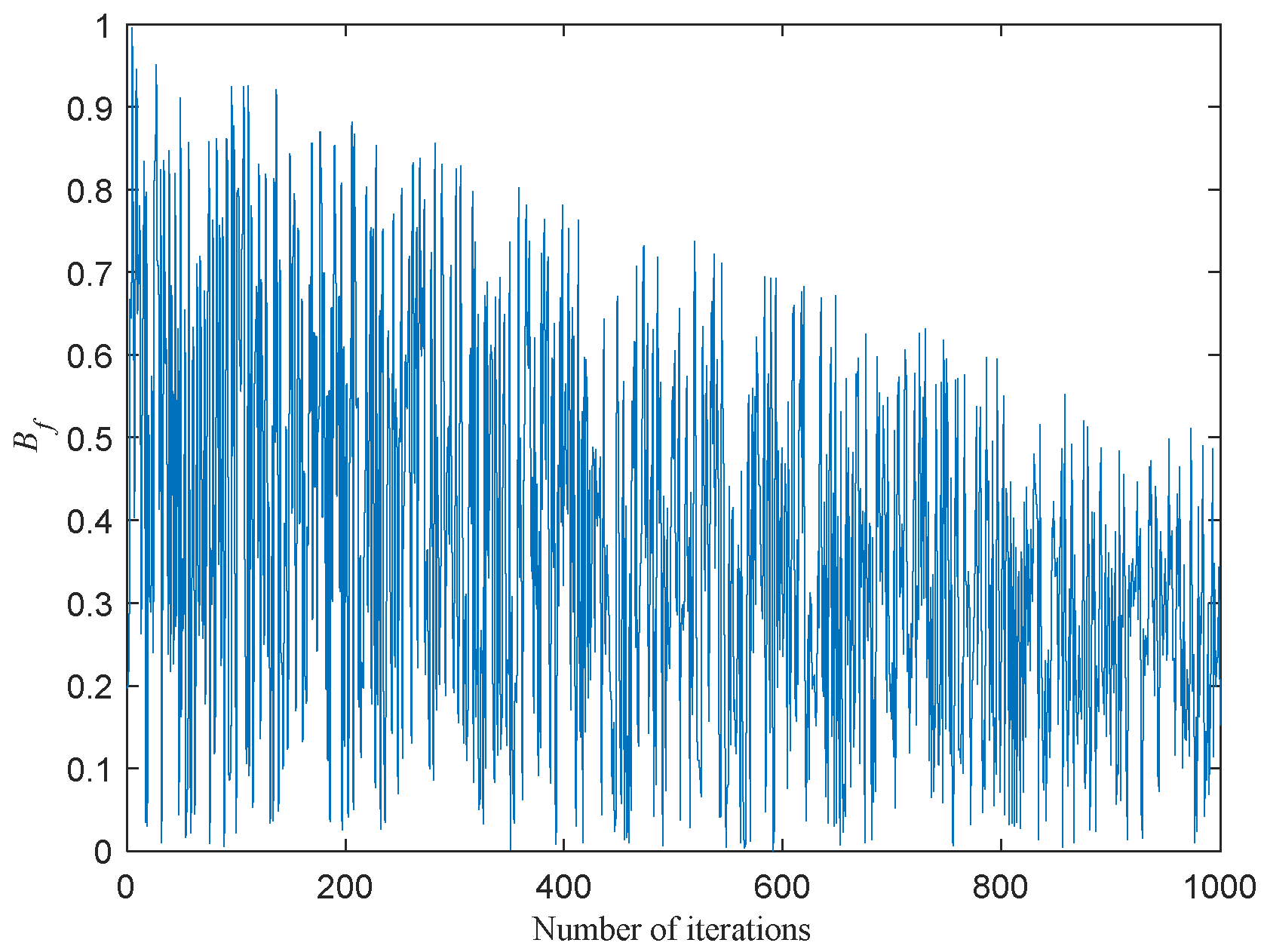
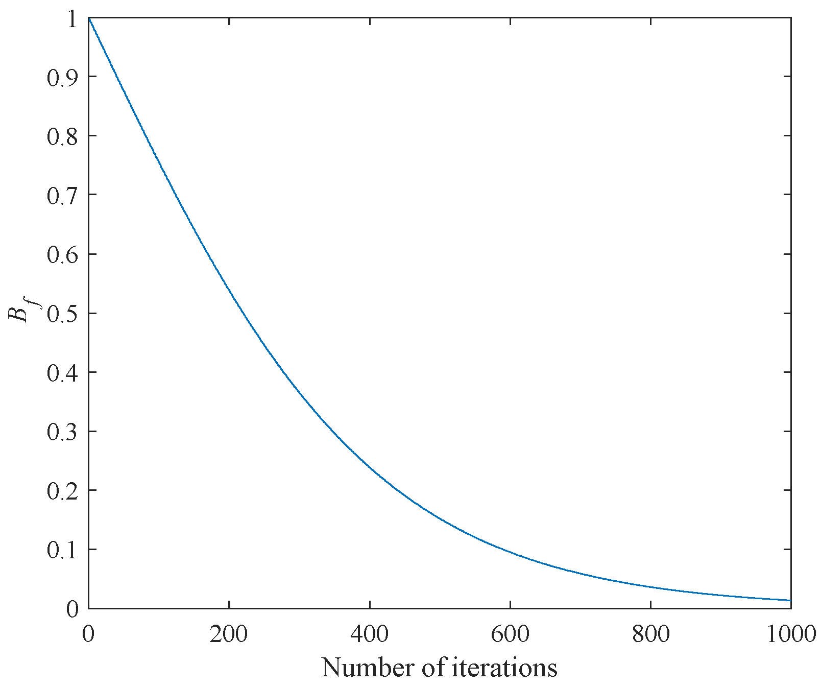
2.1.1. Control Parameters Based on S-Shaped Function
2.1.2. Danger Sensing Mechanism
2.1.3. Dynamic Foraging Mechanism
2.1.4. Improved Whale Fall Strategy
2.1.5. The Flowchart of DSBWO
| Algorithm 1: DSBWO |
| Input: N, D ST, vb,Tmax, UB, LB; Output: the best solution Xbest; |
| 1. The initial population X is generated according to Equation (14). 2. Evaluate the population and find the optimal individual Xbest. 3. t = 1; |
| 4. while (t < Tmax) 5. for i = 1: N 6. Calculate the Bf according to Equation (1). 7. if Bf > 0.5% Exploration phase 8. Update the position of the i-th using danger sensing mechanism in Equation (7). 9. Else %Exploitation phase 10. Update the position of the i-th using dynamic foraging mechanism in Equation (8). 11. End if 12. Calculate and rank the fitness values of beluga whales in the population. 13. Find the beluga whales in the best Xbest, middle Xmid, and worst Xworst positions. 14. Calculate the Wf according to Equation (11). 15. if Bf ≤ Wf % Whale fall phase 16. Update X according Equation (12). 17. End if 18. End for 19. t = t + 1. 20. End while |
2.1.6. Complexity Analysis
2.2. Thresholding Methods
3. Experimental Setup
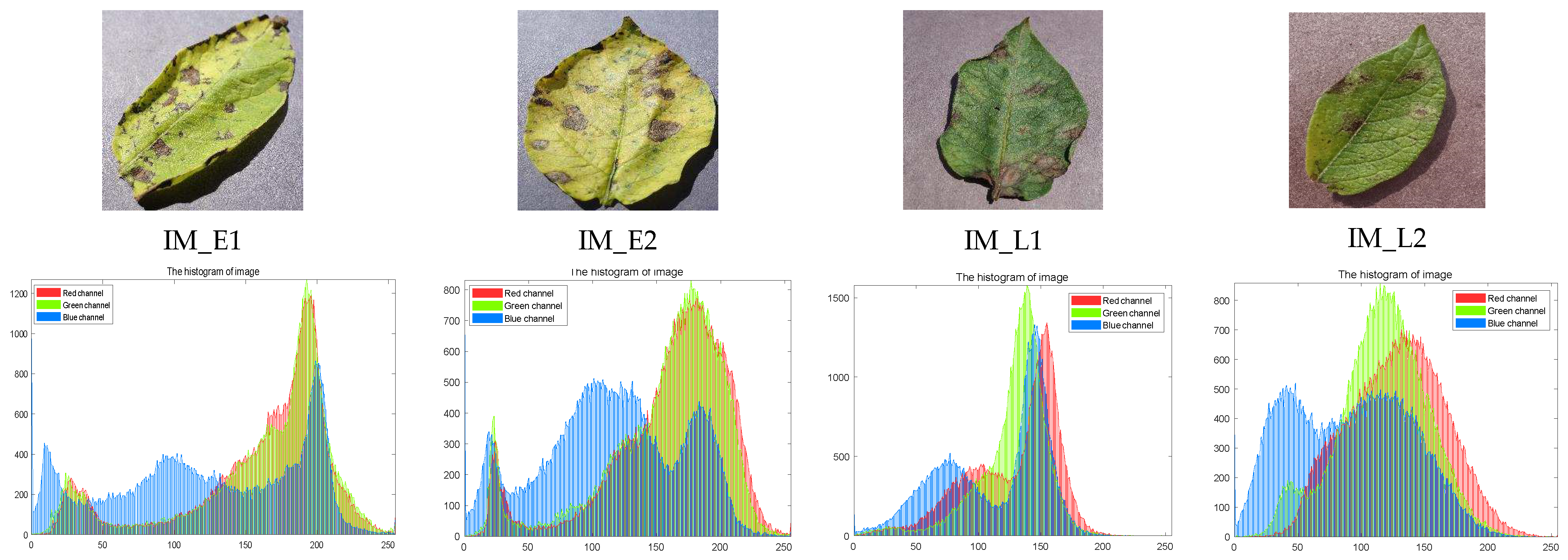
3.1. Experimental Preparation
3.2. Performance Measures
4. Results
4.1. Statistical Results for CEC 2017
4.1.1. Analysis of CEC 2017 Statistical Results
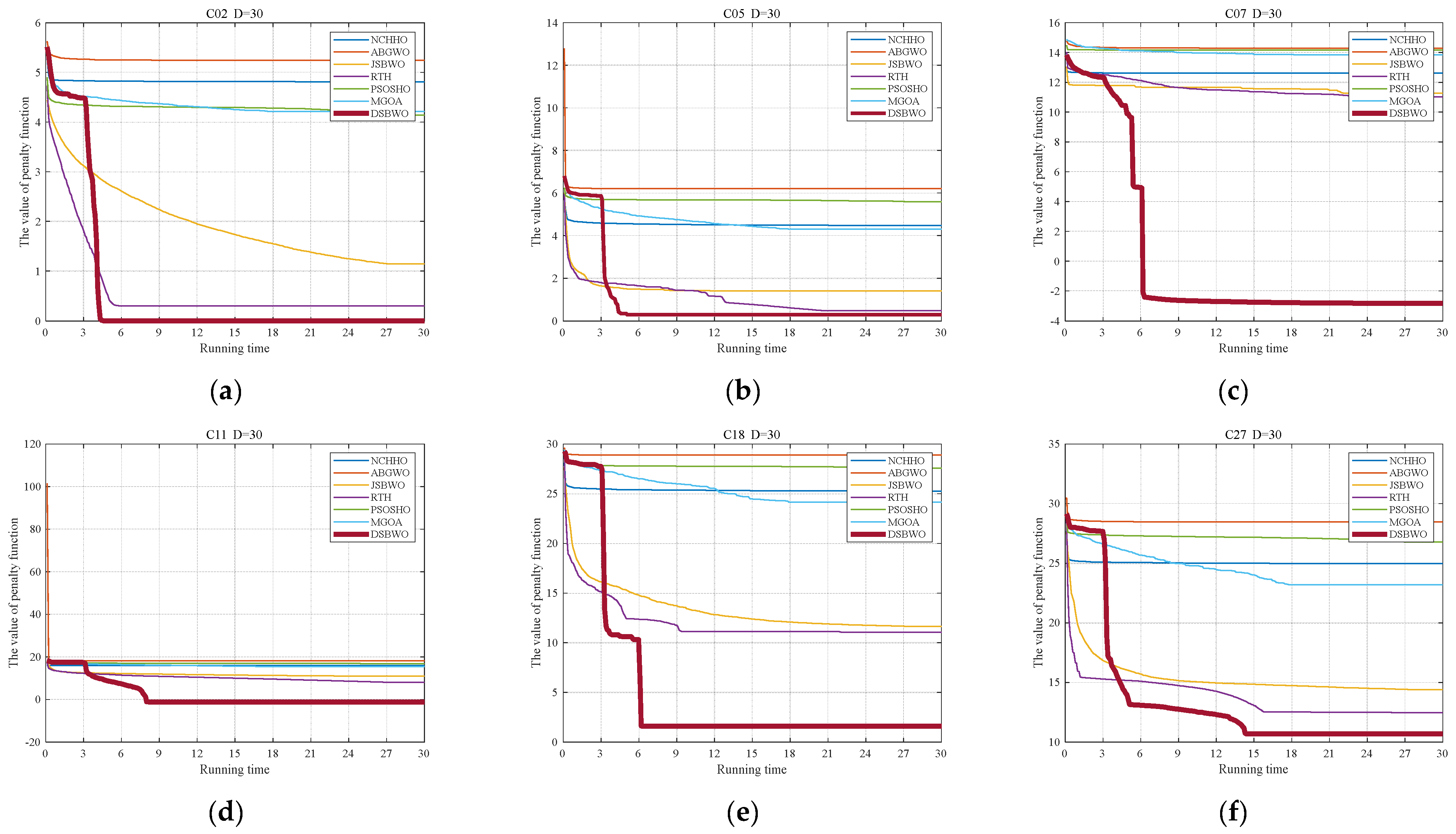
4.1.2. Convergence Curve Analysis
4.2. Otsu Segmentation Experiment Results
4.3. Results of Otsu–Sobel Collaborative Segmentation of Potato Disease Images
4.4. Collaborative Segmentation Experiments Under Different Noise Intensities
4.5. Discussion
5. Conclusions
Supplementary Materials
Author Contributions
Funding
Institutional Review Board Statement
Data Availability Statement
Acknowledgments
Conflicts of Interest
References
- Liu, Y.; Feng, H.; Yue, J.; Li, Z.; Yang, G.; Song, X.; Yang, X.; Zhao, Y. Remote-sensing estimation of potato above-ground biomass based on spectral and spatial features extracted from high-definition digital camera images. Comput. Electron. Agric. 2022, 198, 107089. [Google Scholar] [CrossRef]
- Xu, X.; Pan, S.; Cheng, S.; Zhang, B.; Mu, D.; Ni, P.; Zhang, G.; Yang, S.; Li, R.; Wang, J.; et al. Genome sequence and analysis of the tuber crop potato. Nature 2011, 475, 189–195. [Google Scholar] [PubMed]
- Ray, S.S.; Jain, N.; Arora, R.K.; Chavan, S.; Panigrahy, S. Utility of Hyperspectral Data for Potato Late Blight Disease Detection. J. Indian Soc. Remote Sens. 2011, 39, 161–169. [Google Scholar] [CrossRef]
- Kaitlin, M.G.; Philip, A.T.; Adam, C.; Ittai, H.; John, J.C.; Eric, L.; Gevens, A.J. Hyperspectral Measurements Enable Pre-Symptomatic Detection and Differentiation of Contrasting Physiological Effects of Late Blight and Early Blight in Potato. Remote Sens. 2020, 2, 286. [Google Scholar]
- Franceschini, M.H.D.; Bartholomeus, H.; Van Apeldoorn, D.F.; Suomalainen, J.; Kooistra, L. Feasibility of Unmanned Aerial Vehicle Optical Imagery for Early Detection and Severity Assessment of Late Blight in Potato. Remote Sens. 2019, 11, 224. [Google Scholar] [CrossRef]
- Lees, A.K.; Anne, H. Black dot (Colletotrichum coccodes): An increasingly important disease of potato. Plant Pathol. 2003, 52, 3–12. [Google Scholar] [CrossRef]
- Bueno, A.d.F.; Sutil, W.P.; Jahnke, S.M.; Carvalho, G.A.; Cingolani, M.F.; Colmenarez, Y.C.; Corniani, N. Biological Control as Part of the Soybean Integrated Pest Management (IPM): Potential and Challenges. Agronomy 2023, 13, 2532. [Google Scholar] [CrossRef]
- FAO. Making agrifood systems more resilient to shocks and stresses. In The State of Food and Agriculture 2021; FAO: Rome, Italy, 2021. [Google Scholar]
- Yang, C. Remote Sensing and Precision Agriculture Technologies for Crop Disease Detection and Management with a Practical Application Example. Engineering 2020, 6, 528–532. [Google Scholar] [CrossRef]
- Ding, W.; Abdel-Basset, M.; Alrashdi, I.; Hawash, H. Next generation of computer vision for plant disease monitoring in precision agriculture: A contemporary survey, taxonomy, experiments, and future direction. Inf. Sci. 2024, 665, 120338. [Google Scholar] [CrossRef]
- Lv, P.; Xu, H.; Zhang, Y.; Zhang, Q.; Pan, Q.; Qin, Y.; Chen, Y.; Cao, D.; Wang, J.; Zhang, M.; et al. An Improved Multi-Scale Feature Extraction Network for Rice Disease and Pest Recognition. Insects 2024, 15, 827. [Google Scholar] [CrossRef]
- Song, H.; Wang, J.; Bei, J.; Wang, M. Modified snake optimizer based multi-level thresholding for color image segmentation of agricultural diseases. Expert Syst. Appl. 2024, 255, 124624. [Google Scholar] [CrossRef]
- Anne-Katrin, M. Plant Disease Detection by Imaging Sensors–Parallels and Specific Demands for Precision Agriculture and Plant Phenotyping. Plant Dis. 2016, 100, 241–251. [Google Scholar]
- Otsu, N. A Threshold Selection Method from Gray-Level Histograms. IEEE Trans. Syst. Man Cybern. 1979, 9, 62–66. [Google Scholar] [CrossRef]
- Kadhim, M.K.; Der, C.S.; Phing, C.C. Enhanced dynamic hand gesture recognition for finger disabilities using deep learning and an optimized Otsu threshold method. Eng. Res. Express 2025, 7, 015228. [Google Scholar] [CrossRef]
- Goulart, J.T.; Bassani, R.A.; Bassani, J.W.M. Application based on the Canny edge detection algorithm for recording contractions of isolated cardiac myocytes. Comput. Biol. Med. 2017, 81, 106–110. [Google Scholar] [CrossRef]
- Chen, D.; Mirebeau, J.M.; Shu, H.; Cohen, L.D. A Region-Based Randers Geodesic Approach for Image Segmentation. Int. J. Comput. Vis. 2023, 132, 349–391. [Google Scholar] [CrossRef]
- Kumar, A.; Kumar, A.; Vishwakarma, A.; Singh, G.K. Multilevel thresholding for crop image segmentation based on recursive minimum cross entropy using a swarm-based technique. Comput. Electron. Agric. 2022, 203, 107488. [Google Scholar] [CrossRef]
- Sankur, B.L.; Sezgin, M. Survey over image thresholding techniques and quantitative performance evaluation. J. Electron. Imaging 2004, 13, 146–168. [Google Scholar] [CrossRef]
- Houssein, E.H.; Hussain, K.; Abualigah, L.; Abd Elaziz, M.; Alomoush, W.; Dhiman, G.; Djenouri, Y.; Cuevas, E. An improved opposition-based marine predators algorithm for global optimization and multilevel thresholding image segmentation. Knowl.-Based Syst. 2021, 229, 107348. [Google Scholar] [CrossRef]
- Serbet, F.; Kaya, T. New comparative approach to multi-level thresholding: Chaotically initialized adaptive meta-heuristic optimization methods. Neural Comput. Appl. 2025, 37, 8371–8396. [Google Scholar] [CrossRef]
- Odiathevar, M.; Seah, W.K.G.; Frean, M. A Bayesian Approach To Distributed Anomaly Detection In Edge AI Networks. IEEE Trans. Parallel Distrib. Syst. 2022, 33, 3306–3320. [Google Scholar] [CrossRef]
- Zhu, D.; Shen, J.; Zheng, Y.; Li, R.; Zhou, C.; Cheng, S.; Yao, Y. Multi-strategy learning-based particle swarm optimization algorithm for COVID-19 threshold segmentation. Comput. Biol. Med. 2024, 176, 108498. [Google Scholar] [CrossRef]
- Rahaman, J.; Sing, M. An efficient multilevel thresholding based satellite image segmentation approach using a new adaptive cuckoo search algorithm. Expert Syst. Appl. 2021, 174, 114633. [Google Scholar] [CrossRef]
- Kong, W.; Chen, J.; Song, Y.; Fang, Z.; Yang, X.; Zhang, H. Sobel Edge Detection Algorithm with Adaptive Threshold based on Improved Genetic Algorithm for Image Processing. Int. J. Adv. Comput. Sci. Appl. 2023, 14, 557–562. [Google Scholar] [CrossRef]
- Abd Elaziz, M.; Ewees, A.A.; Oliva, D. Hyper-heuristic method for multilevel thresholding image segmentation. Expert Syst. Appl. 2020, 146, 113201. [Google Scholar] [CrossRef]
- Qadri, S.A.A.; Huang, N.F.; Wani, T.M.; Bhat, S.A. Advances and Challenges in Computer Vision for Image-Based Plant Disease Detection: A Comprehensive Survey of Machine and Deep Learning Approaches. IEEE Trans. Autom. Sci. Eng. 2024, 22, 2639–2670. [Google Scholar] [CrossRef]
- Kim, K.S.; Yoo, B.H.; Shelia, V.; Porter, C.H.; Hoogenboom, G. START: A data preparation tool for crop simulation models using web-based soil databases. Comput. Electron. Agric. 2018, 154, 256–264. [Google Scholar] [CrossRef]
- Zhong, C.; Li, G.; Meng, Z. Beluga whale optimization: A novel nature-inspired metaheuristic algorithm. Knowl. Based Syst. 2022, 251, 109215. [Google Scholar] [CrossRef]
- Yuan, X.; Hu, G.; Zhong, J.; Wei, G. HBWO-JS: Jellyfish search boosted hybrid beluga whale optimization algorithm for engineering applications. J. Comput. Des. Eng. 2023, 10, 1615–1656. [Google Scholar] [CrossRef]
- Shen, X.; Wu, Y.; Li, L.; Zhang, T. A modified adaptive beluga whale optimization based on spiral search and elitist strategy for short-term hydrothermal scheduling. Electr. Power Syst. Res. 2023, 228, 110051. [Google Scholar] [CrossRef]
- Feng, O.Y.; Chen, Y.; Han, Q.; Carroll, R.J.; Samworth, R.J. Nonparametric, Tuning-Free Estimation of S-Shaped Functions. J. R. Stat. Soc. Ser. B Stat. Methodol. 2022, 84, 1324–1352. [Google Scholar] [CrossRef]
- Yang, P.; Hu, Z.; Zhou, Y.; Su, Q.; Xiong, W. Grey prediction evolution algorithm with a dominator guidance strategy for solving multi-level image thresholding. Appl. Soft Comput. 2025, 174, 112947. [Google Scholar] [CrossRef]
- Liu, X.; Zhang, Z.; Hao, Y.; Zhao, H.; Yang, Y. Optimized OTSU Segmentation Algorithm-Based Temperature Feature Extraction Method for Infrared Images of Electrical Equipment. Sensors 2024, 24, 1126. [Google Scholar] [CrossRef]
- Moussa, M.; Guedri, W.; Douik, V.A. A Novel Metaheuristic Algorithm for Edge Detection Based on Artificial Bee Colony Technique. Trait. Du Signal 2020, 37, 405–412. [Google Scholar] [CrossRef]
- Li, Z. Optimized image registration algorithm at subpixel level for Geostationary Operational Environmental Satellite-R Advanced Baseline Imager navigation and registration performance assessment. J. Appl. Remote Sens. 2023, 17, 026504. [Google Scholar] [CrossRef]
- Fan, T. Research on Edge Detection of Agricultural Pest and Disease Leaf Image Based on LVQ Neural Network. Recent Adv. Comput. Sci. Commun. 2021, 14, 1903–1911. [Google Scholar] [CrossRef]
- Yadav, G.S.; Sathish, T.; Suresh, G.R. Detection of fire in forest area using chromatic measurements by Sobel edge detection algorithm compared with Prewitt gradient edge detector. AIP Conf. Proc. 2024, 2853, 020221. [Google Scholar]
- Song, H.; Wang, J.; Song, L.; Zhang, H.; Bei, J.; Ni, J.; Ye, B. Improvement and application of hybrid real-coded genetic algorithm. Appl. Intell. 2022, 52, 17410–17448. [Google Scholar] [CrossRef]
- Wang, J.; Bei, J.; Song, H.; Zhang, H.; Zhang, P. A whale optimization algorithm with combined mutation and removing similarity for global optimization and multilevel thresholding image segmentation. Appl. Soft Comput. 2023, 137, 110130. [Google Scholar] [CrossRef]
- Dehkordi, A.A.; Sadiq, A.S.; Mirjalili, S.; Ghafoor, K.Z. Nonlinear-based Chaotic Harris Hawks Optimizer: Algorithm and Internet of Vehicles application. Appl. Soft Comput. 2021, 109, 107574. [Google Scholar] [CrossRef]
- Wang, J.; Lin, D.; Zhang, Y.; Huang, S. An adaptively balanced grey wolf optimization algorithm for feature selection on high-dimensional classification. Eng. Appl. Artif. Intell. 2022, 114, 105088. [Google Scholar] [CrossRef]
- Ferahtia, S.; Houari, A.; Rezk, H.; Djerioui, A.; Machmoum, M.; Motahhir, S.; Ait-Ahmed, M. Red-tailed hawk algorithm for numerical optimization and real-world problems. Sci. Rep. 2023, 13, 12950. [Google Scholar] [CrossRef] [PubMed]
- Hasanien, H.M.; Alsaleh, I.; Tostado-Veliz, M.; Zhang, M.; Alateeq, A.; Jurado, F.; Alassaf, A. Hybrid particle swarm and sea horse optimization algorithm-based optimal reactive power dispatch of power systems comprising electric vehicles. Energy 2024, 286, 129583. [Google Scholar] [CrossRef]
- Ingle, K.K.; Jatoth, R.K. Non-linear channel equalization using modified grasshopper optimization algorithm. Appl. Soft Comput. 2024, 153, 110091. [Google Scholar] [CrossRef]
- Huynh-Thu, Q.; Ghanbari, M. Scope of validity of PSNR in image/video quality assessment. Electron. Lett. 2008, 44, 800–801. [Google Scholar] [CrossRef]
- Wang, Z.; Bovik, A.C.; Sheikh, H.R.; Simoncelli, E.P. Image quality assessment: From error visibility to structural similarity. IEEE Trans Image Process 2004, 13, 600–612. [Google Scholar] [CrossRef]
- Zhang, L.; Huang, Z.; Yang, Z.; Yang, B.; Yu, S.; Zhao, S.; Zhang, X.; Li, X.; Yang, H.; Lin, Y.; et al. Tomato Stem and Leaf Segmentation and Phenotype Parameter Extraction Based on Improved Red Billed Blue Magpie Optimization Algorithm. Agriculture 2025, 15, 180. [Google Scholar] [CrossRef]
- Friedman, M. A Comparison of Alternative Tests of Significance for the Problem of $m$ Rankings. Ann. Math. Stat. 1940, 11, 86–92. [Google Scholar] [CrossRef]
- Liao, C.; Li, S.; Luo, Z. Gene Selection Using Wilcoxon Rank Sum Test and Support Vector Machine for Cancer Classification. In Lecture Notes in Computer Science, Proceedings of the Computational Intelligence and Security (CIS 2006), Guangzhou, China, 3–6 November 2006; Springer: Berlin/Heidelberg, Germany, 2006. [Google Scholar]


| Algorithm | References | Parameters |
|---|---|---|
| NCHHO | [41] | E0 = [0, 1]. |
| ABGWO | [42] | A = [−2, 2], C = [0, 2]; |
| JSBWO | [30] | φ = [0, 1], γ = 1, α = 3, β r = [0, 1]. |
| RTH | [43] | s = 0.01, β = 1.5, A = 15, R0 = 0.5. |
| PSOSHO | [44] | s = 0.01, p = 0.5, u = 0.5, v = 0.5. |
| MGOA | [45] | Cmin = 0.0001, Cmax = 1, l = 1.5, β = 0.4. |
| DSBWO | - | ST = [0, 0.3], vb = [−1, 1]. |
| Image | TH | NCHHO | ABGWO | JSBWO | RTH | PSOSHO | MGOA | DSBWO |
|---|---|---|---|---|---|---|---|---|
| Friedman mean rank | 2.625 | 3.6 | 4.68 | 4.75 | 2.9375 | 2.5 | 7 | |
| Rank | 6 | 4 | 3 | 2 | 5 | 7 | 1 | |
| Dimension | Significant Level | χ2 | p-Value | Null Hypothesis | Alternative Hypothesis | |
|---|---|---|---|---|---|---|
| D = 30 | α = 0.05 | 133.18 | 12.59 | 2.7508 × 10⁻²⁶ | Reject | Accept |
| Comparison | w | t | l | p-Value | Significance |
|---|---|---|---|---|---|
| DSBWO vs. NCHHO | 28 | 0 | 0 | 4.6471 × 10⁻⁶ | Yes |
| DSBWO vs. ABGWO | 27 | 0 | 1 | 1.6445 × 10⁻⁷ | Yes |
| DSBWO vs. JSBWO | 23 | 0 | 5 | 0.03382 | Yes |
| DSBWO vs. RTH | 25 | 0 | 3 | 0.1469 | No |
| DSBWO vs. PSOSHO | 28 | 0 | 0 | 5.5521 × 10⁻⁷ | Yes |
| DSBWO vs. MGOA | 28 | 0 | 0 | 1.6961 × 10⁻⁵ | Yes |
| Algorithms | NCHHO | ABGWO | JSBWO | RTH | PSOSHO | MGOA | DSBWO |
|---|---|---|---|---|---|---|---|
| Friedman mean rank | 2.625 | 3.6 | 4.68 | 4.75 | 2.9375 | 2.5 | 7 |
| Rank | 6 | 4 | 3 | 2 | 5 | 7 | 1 |
| TH | NCHHO | ABGWO | JSBWO | RTH | PSOSHO | MGOA | DSBWO | |||||||
|---|---|---|---|---|---|---|---|---|---|---|---|---|---|---|
| PSNR | SSIM | PSNR | SSIM | PSNR | SSIM | PSNR | SSIM | PSNR | SSIM | PSNR | SSIM | PSNR | SSIM | |
| 4 | 3.7 | 4.3 | 2.2 | 3.7 | 4.5 | 4.7 | 5.7 | 3.3 | 3.2 | 2.8 | 2 | 2.7 | 6.7 | 6.5 |
| 8 | 4.3 | 3.9 | 3.2 | 3.9 | 4.9 | 3.3 | 2.6 | 3.7 | 3.1 | 3.9 | 3 | 2.3 | 6.9 | 7 |
| 15 | 4.5 | 3.1 | 3.5 | 4.2 | 3.6 | 4.8 | 4.1 | 3.7 | 3.3 | 2.8 | 2.5 | 2.7 | 6.5 | 6.65 |
| 20 | 3.7 | 3.8 | 2.4 | 4.3 | 5.1 | 5.4 | 4.2 | 2.9 | 3.5 | 3.3 | 2.5 | 2.9 | 6.6 | 6.8 |
| TH | χ2 | p-Value | Null Hypothesis | Alternative Hypothesis | |
|---|---|---|---|---|---|
| 4 | 42.77 | 12.59 | 1.2944 × 10⁻⁷ | Reject | Accept |
| 8 | 30.39 | 12.59 | 3.3197 × 10⁻⁵ | Reject | Accept |
| 15 | 27.09 | 12.59 | 1.0000 × 10⁻⁴ | Reject | Accept |
| 20 | 36.16 | 12.59 | 6.2733 × 10⁻⁶ | Reject | Accept |
| TH | NCHHO vs. DSBWO | ABGWO vs. DSBWO | JSBWO vs. DSBWO | RTH vs. DSBWO | PSOSHO vs. DSBWO | MGOA vs. DSBWO | ||||||
|---|---|---|---|---|---|---|---|---|---|---|---|---|
| p | h | p | h | p | h | p | h | p | h | p | h | |
| 4 | 0.0290 | 1 | 0.0409 | 1 | 0.0513 | 0 | 0.0413 | 1 | 0.0013 | 1 | 0.0172 | 1 |
| 8 | 0.0452 | 1 | 0.0113 | 1 | 0.0173 | 1 | 0.0257 | 1 | 0.0091 | 1 | 0.0091 | 1 |
| 15 | 0.0211 | 1 | 0.0211 | 1 | 0.0022 | 1 | 0.0073 | 1 | 0.0257 | 1 | 0.0257 | 1 |
| 20 | 0.0211 | 1 | 0.0173 | 1 | 0.0257 | 1 | 0.0064 | 1 | 0.0312 | 1 | 0.0036 | 1 |
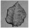
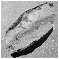
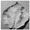
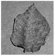
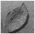
| Image | TH = 4 | TH = 8 | TH = 15 | TH = 20 |
|---|---|---|---|---|
| IM_E1 |  |  |  |  |
 |  |  |  | |
 |  |  |  | |
| IM_E2 |  |  |  |  |
 |  |  |  | |
 |  |  |  | |
| IM_L1 |  |  |  |  |
 |  |  |  | |
 |  |  |  | |
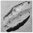
| IM_L2 |  |  |  |  |
 |  |  |  | |
 |  |  |  |
| Algorithms | NCHHO | ABGWO | JSBWO | RTH | PSOSHO | MGOA | DSBWO |
|---|---|---|---|---|---|---|---|
| Friedman mean rank | 2.625 | 3.6 | 4.68 | 4.75 | 2.9375 | 2.5 | 7 |
| Rank | 6 | 4 | 3 | 2 | 5 | 7 | 1 |
| Image | NCHHO | ABGWO | JSBWO | RTH | PSOSHO | MGOA | DSBWO | |||||||
|---|---|---|---|---|---|---|---|---|---|---|---|---|---|---|
| PSNR | SSIM | PSNR | SSIM | PSNR | SSIM | PSNR | SSIM | PSNR | SSIM | PSNR | SSIM | PSNR | SSIM | |
| IM_E1 | 3.75 | 3 | 3.5 | 4.375 | 3.5 | 4.7 | 5 | 4.5 | 3.75 | 2.375 | 1.75 | 2.875 | 6.75 | 7 |
| IM_E2 | 3 | 2. 875 | 3.25 | 4.375 | 4.5 | 3.3 | 3.25 | 6 | 4 | 3.875 | 3 | 2 | 7 | 6.75 |
| IM_L1 | 3 | 3.25 | 4.5 | 4 | 3.25 | 4.8 | 5.75 | 5.25 | 3.5 | 3 | 1.75 | 1.75 | 6.25 | 7 |
| IM_L2 | 3 | 2 | 2.4 | 3.25 | 2.75 | 5.4 | 4.75 | 6 | 4 | 4.5 | 3.5 | 3 | 7 | 7 |
| Image | NCHHO | ABGWO | JSBWO | RTH | PSOSHO | MGOA | DSBWO | |||||||
|---|---|---|---|---|---|---|---|---|---|---|---|---|---|---|
| IoU | CPU | IoU | CPU | IoU | CPU | IoU | CPU | IoU | CPU | IoU | CPU | IoU | CPU | |
| IM_E1 | 0.8541 | 1.782 | 0.89544 | 1.783 | 0.8409 | 1.793 | 0.8797 | 1.787 | 0.8442 | 1.778 | 0.8525 | 1.768 | 0.8769 | 1.763 |
| IM_E2 | 0.8654 | 1.791 | 0.8614 | 1.846 | 0.8650 | 1.802 | 0.8617 | 1.792 | 0.8539 | 1.811 | 0.8607 | 1.782 | 0.8716 | 1.771 |
| IM_L1 | 0.8613 | 1.867 | 0.8561 | 1.875 | 0.8676 | 1.851 | 0.8733 | 1.873 | 0.8685 | 1.855 | 0.8573 | 1.854 | 0.8828 | 1.830 |
| IM_L2 | 0.8692 | 1.914 | 0.8683 | 1.871 | 0.8476 | 1877 | 0.8721 | 1.866 | 0.8613 | 1.872 | 0.8638 | 1.865 | 0.8867 | 1.851 |
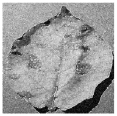
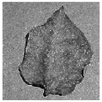
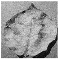
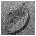
| Image | IM_E1 | IM_E2 | IM_L1 | IM_L2 |
|---|---|---|---|---|
| p = 0.01 | 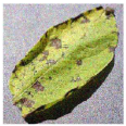 | 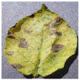 |  | 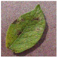 |
 |  |  |  | |
| p = 0.02 | 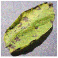 | 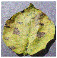 | 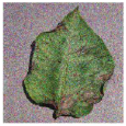 |  |
 |  |  | 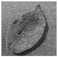 | |
| p = 0.03 | 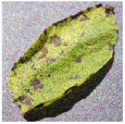 |  | 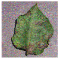 | 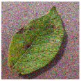 |
 |  |  |  |
| Image | p | NCHHO | ABGWO | JSBWO | RTH | PSOSHO | MGOA | DSBWO | |||||||
|---|---|---|---|---|---|---|---|---|---|---|---|---|---|---|---|
| PSNR | SSIM | PSNR | SSIM | PSNR | SSIM | PSNR | SSIM | PSNR | SSIM | PSNR | SSIM | PSNR | SSIM | ||
| IM_E1 | 0.01 | 31.08 | 0.8482 | 30.74 | 0.8283 | 30.48 | 0.8443 | 31.17 | 0.8760 | 31.02 | 0.8278 | 30.85 | 0.8068 | 31.29 | 0.8653 |
| 0.02 | 30.73 | 0.8134 | 30.15 | 0.8007 | 30.12 | 0.8122 | 30.80 | 0.8541 | 30.64 | 0.8093 | 30.17 | 0.8005 | 31.01 | 0.8432 | |
| 0.03 | 29.68 | 0.7912 | 28.92 | 0.7824 | 29.83 | 0.8001 | 30.42 | 0.8223 | 30.20 | 0.8001 | 29.69 | 0.7946 | 30.78 | 0.8221 | |
| IM_E2 | 0.01 | 32.20 | 0.8291 | 32.34 | 0.8546 | 32.30 | 0.8342 | 32.37 | 0.8479 | 32.19 | 0.8221 | 32.17 | 0.8271 | 32.40 | 0.8571 |
| 0.02 | 32.01 | 0.8132 | 31.71 | 0.8233 | 32.11 | 0.8240 | 32.15 | 0.8236 | 31.23 | 0.8097 | 32.01 | 0.8128 | 32.22 | 0.8468 | |
| 0.03 | 31.55 | 0.8062 | 31.34 | 0.8071 | 31.96 | 0.8102 | 32.02 | 0.8134 | 31.14 | 0.8003 | 31.54 | 0.8060 | 32.15 | 0.8324 | |
| IM_L1 | 0.01 | 33.17 | 0.8580 | 33.22 | 0.8619 | 33.07 | 0.8432 | 33.27 | 0.8653 | 33.01 | 0.8407 | 33.08 | 0.8432 | 33.30 | 0.8691 |
| 0.02 | 33.06 | 0.8365 | 33.12 | 0.8434 | 32.86 | 0.8331 | 33.16 | 0.8546 | 32.85 | 0.8235 | 32.91 | 0.8331 | 33.22 | 0.8568 | |
| 0.03 | 32.81 | 0.8173 | 32.94 | 0.8208 | 32.53 | 0.8023 | 33.02 | 0.8301 | 32.45 | 0.8010 | 32.62 | 0.8023 | 33.14 | 0.8423 | |
| IM_L2 | 0.01 | 30.36 | 0.8617 | 30.32 | 0.8608 | 30.37 | 0.8701 | 30.42 | 0.8726 | 30.29 | 0.8602 | 30.35 | 0.8615 | 30.44 | 0.8728 |
| 0.02 | 30.20 | 0.8562 | 30.11 | 0.8524 | 30.15 | 0.8526 | 30.25 | 0.8623 | 30.13 | 0.8515 | 30.21 | 0.8562 | 30.27 | 0.8630 | |
| 0.03 | 29.92 | 0.8513 | 29.88 | 0.8503 | 29.86 | 0.8502 | 30.13 | 0.8547 | 29.84 | 0.8501 | 29.94 | 0.8515 | 30.16 | 0.8551 | |
| Image | p | NCHHO | ABGWO | JSBWO | RTH | PSOSHO | MGOA | DSBWO | |||||||
|---|---|---|---|---|---|---|---|---|---|---|---|---|---|---|---|
| IoU | CPU | IoU | CPU | IoU | CPU | IoU | CPU | IoU | CPU | IoU | CPU | IoU | CPU | ||
| IM_E1 | 0.01 | 0.8540 | 1.822 | 0.8544 | 1.830 | 0.8531 | 1.829 | 0.8557 | 1.817 | 0.8532 | 1.828 | 0.8534 | 1.819 | 0.8559 | 1.813 |
| 0.02 | 0.8532 | 1.825 | 0.8537 | 1.833 | 0.8517 | 1.831 | 0.8544 | 1.821 | 0.8523 | 1.831 | 0.8526 | 1.824 | 0.8548 | 1.820 | |
| 0.03 | 0.8517 | 1.837 | 0.8518 | 1.846 | 0.8492 | 1.842 | 0.8523 | 1.834 | 0.8504 | 1.844 | 0.8505 | 1.835 | 0.8530 | 1.831 | |
| IM_E2 | 0.01 | 0.8643 | 1.841 | 0.8633 | 1.846 | 0.8644 | 1.842 | 0.8647 | 1.840 | 0.8554 | 1.841 | 0.8621 | 1.844 | 0.8661 | 1.840 |
| 0.02 | 0.8626 | 1.850 | 0.8628 | 1.852 | 0.8624 | 1.848 | 0.8634 | 1.846 | 0.8543 | 1.847 | 0.8613 | 1.849 | 0.8654 | 1.845 | |
| 0.03 | 0.8608 | 1.857 | 0.8604 | 1.858 | 0.8606 | 1.856 | 0.8601 | 1.853 | 0.8529 | 1.855 | 0.8594 | 1.858 | 0.8638 | 1.853 | |
| IM_L1 | 0.01 | 0.8543 | 1.877 | 0.8554 | 1.875 | 0.8545 | 1.876 | 0.8556 | 1.875 | 0.8545 | 1.878 | 0.8542 | 1.878 | 0.8557 | 1.873 |
| 0.02 | 0.8522 | 1.881 | 0.8542 | 1.880 | 0.8533 | 1.882 | 0.8547 | 1.881 | 0.8536 | 1.883 | 0.8534 | 1.883 | 0.8549 | 1.880 | |
| 0.03 | 0.8507 | 1.893 | 0.8525 | 1.891 | 0.8517 | 1.893 | 0.8521 | 1.891 | 0.8518 | 1.894 | 0.8521 | 1.892 | 0.8530 | 1.889 | |
| IM_L2 | 0.01 | 0.8439 | 1.923 | 0.8436 | 1.921 | 0.8422 | 1.923 | 0.8448 | 1.918 | 0.8434 | 1.922 | 0.8428 | 1.922 | 0.8450 | 1.915 |
| 0.02 | 0.8428 | 1.926 | 0.8428 | 1.923 | 0.8418 | 1.925 | 0.8438 | 1.923 | 0.8425 | 1.927 | 0.8420 | 1.927 | 0.8442 | 1.922 | |
| 0.03 | 0.8413 | 1.932 | 0.8414 | 1.931 | 0.8406 | 1.932 | 0.8427 | 1.930 | 0.8411 | 1.934 | 0.8409 | 1.933 | 0.8331 | 1.930 | |
Disclaimer/Publisher’s Note: The statements, opinions and data contained in all publications are solely those of the individual author(s) and contributor(s) and not of MDPI and/or the editor(s). MDPI and/or the editor(s) disclaim responsibility for any injury to people or property resulting from any ideas, methods, instructions or products referred to in the content. |
© 2025 by the authors. Licensee MDPI, Basel, Switzerland. This article is an open access article distributed under the terms and conditions of the Creative Commons Attribution (CC BY) license (https://creativecommons.org/licenses/by/4.0/).
Share and Cite
Bei, J.-L.; Wang, J.-Q. Edge–Region Collaborative Segmentation of Potato Leaf Disease Images Using Beluga Whale Optimization Algorithm with Danger Sensing Mechanism. Agriculture 2025, 15, 1123. https://doi.org/10.3390/agriculture15111123
Bei J-L, Wang J-Q. Edge–Region Collaborative Segmentation of Potato Leaf Disease Images Using Beluga Whale Optimization Algorithm with Danger Sensing Mechanism. Agriculture. 2025; 15(11):1123. https://doi.org/10.3390/agriculture15111123
Chicago/Turabian StyleBei, Jin-Ling, and Ji-Quan Wang. 2025. "Edge–Region Collaborative Segmentation of Potato Leaf Disease Images Using Beluga Whale Optimization Algorithm with Danger Sensing Mechanism" Agriculture 15, no. 11: 1123. https://doi.org/10.3390/agriculture15111123
APA StyleBei, J.-L., & Wang, J.-Q. (2025). Edge–Region Collaborative Segmentation of Potato Leaf Disease Images Using Beluga Whale Optimization Algorithm with Danger Sensing Mechanism. Agriculture, 15(11), 1123. https://doi.org/10.3390/agriculture15111123