
Early Yield Prediction of Oilseed Rape Using UAV-Based Hyperspectral Imaging Combined with Machine Learning Algorithms


Abstract

1. Introduction
2. Materials and Methods
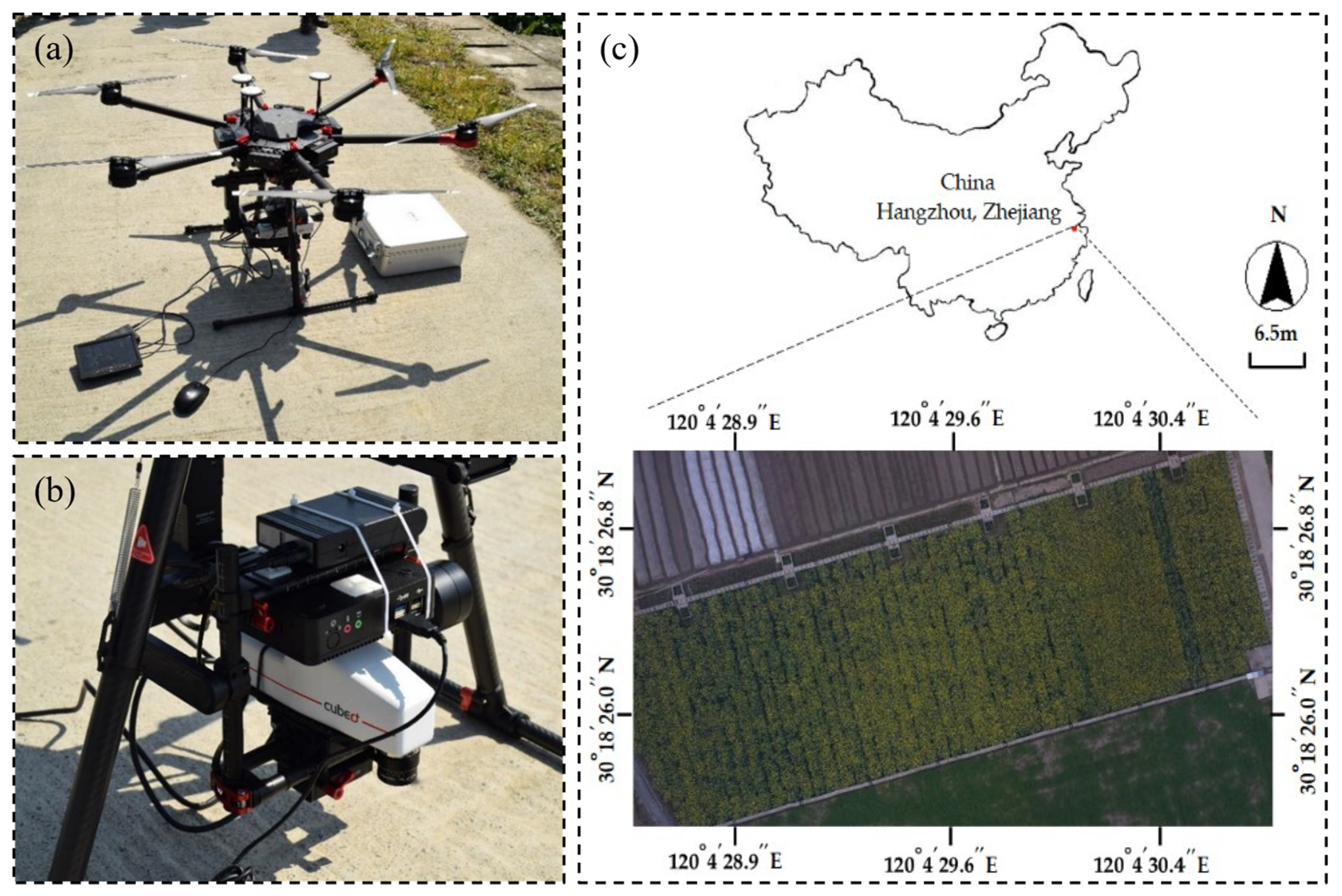
2.1. Experimental Location and Crop Husbandry
2.2. Hyperspectral Imaging Data Acquisition
2.3. Data Processing
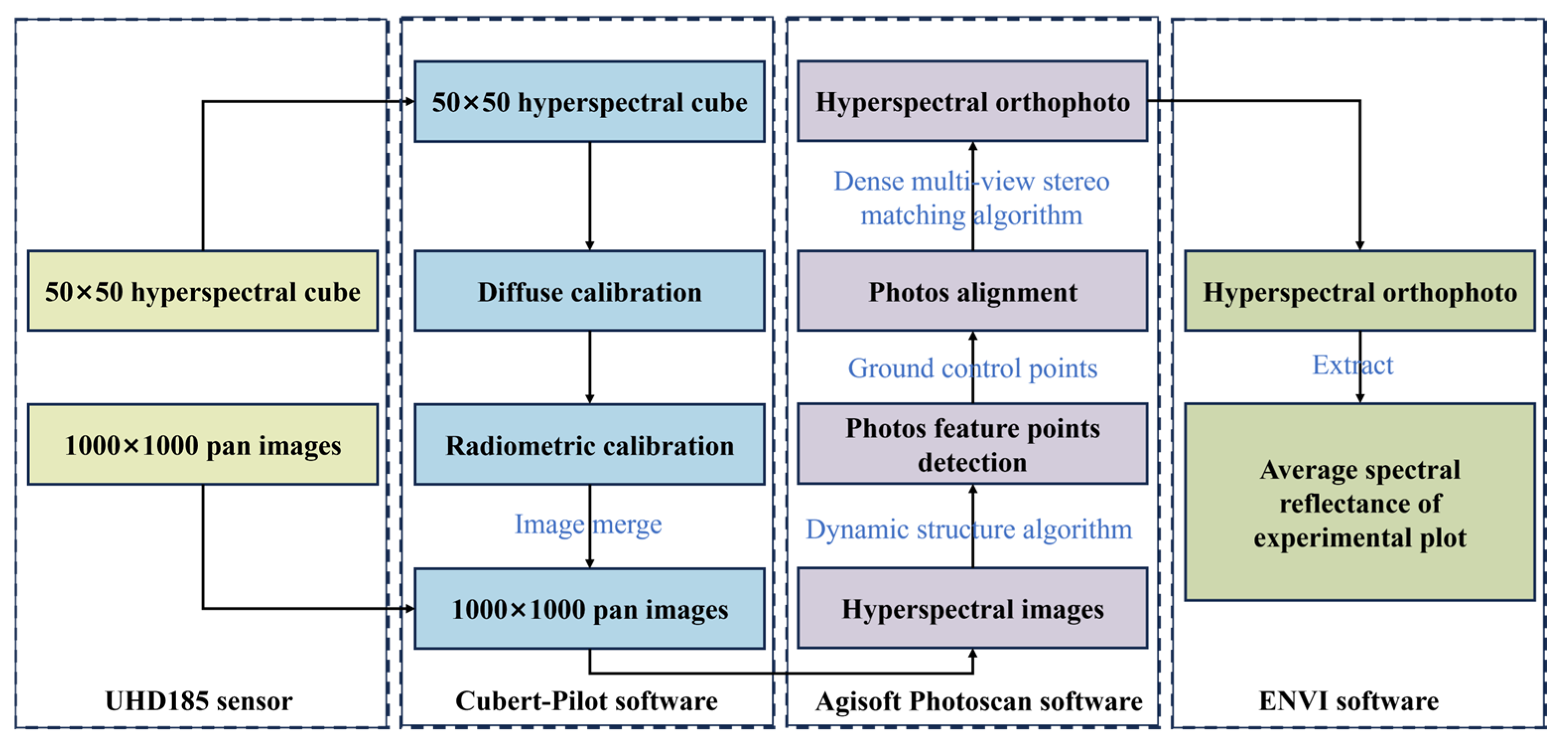
2.3.1. Hyperspectral Remote Sensing Image Processing
2.3.2. Radiation Calibration
2.3.3. Spectral Preprocessing
2.3.4. Wavelength Variable Selection
2.3.5. Vegetation Indices
2.3.6. Machine Learning Algorithms
2.3.7. Model Evaluation
3. Results and Analysis
3.1. Investigating Yield Metrics and Spectral Attributes in Oilseed Rape Treatment
3.1.1. Descriptive Statistics of Measured Yield
3.1.2. The Effect of Different Pretreatment Methods on the Yield Prediction of Oilseed Rape
3.1.3. Analysis of Spectral Features
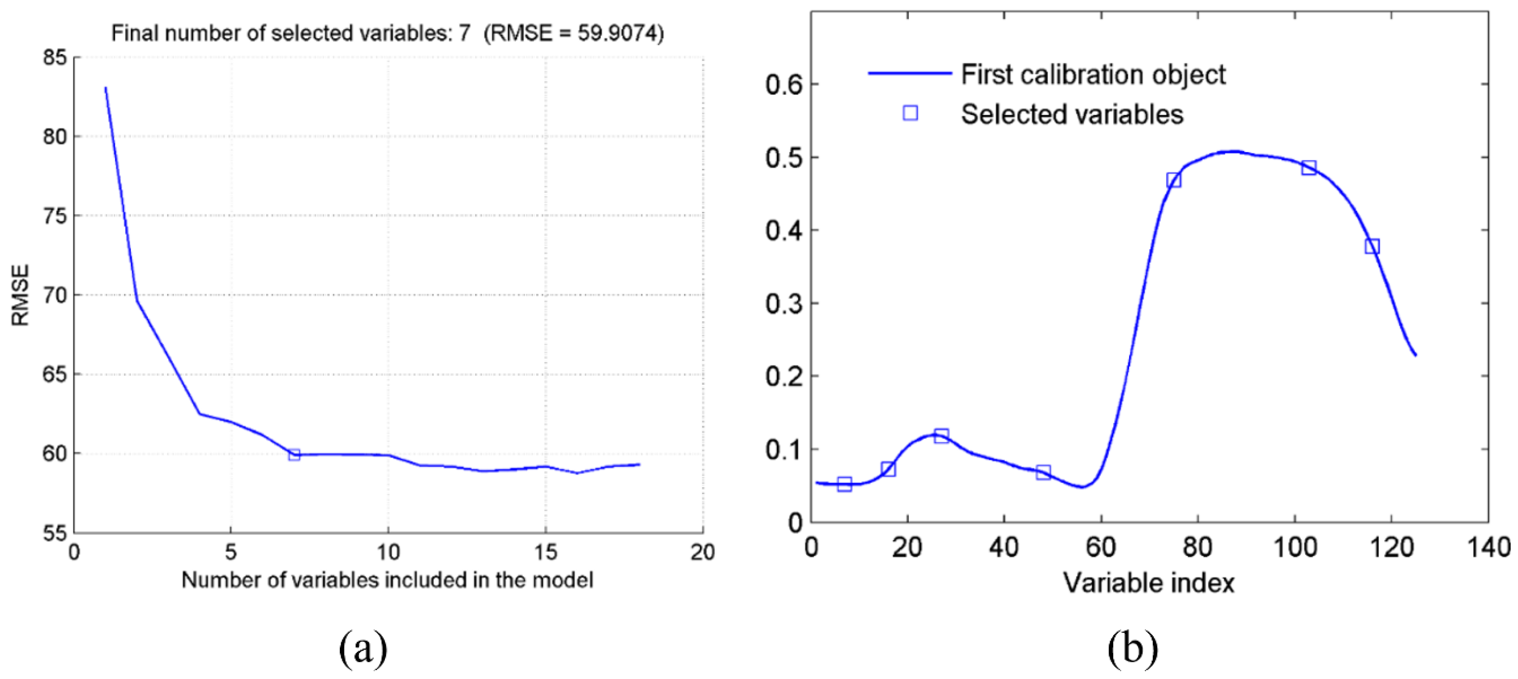
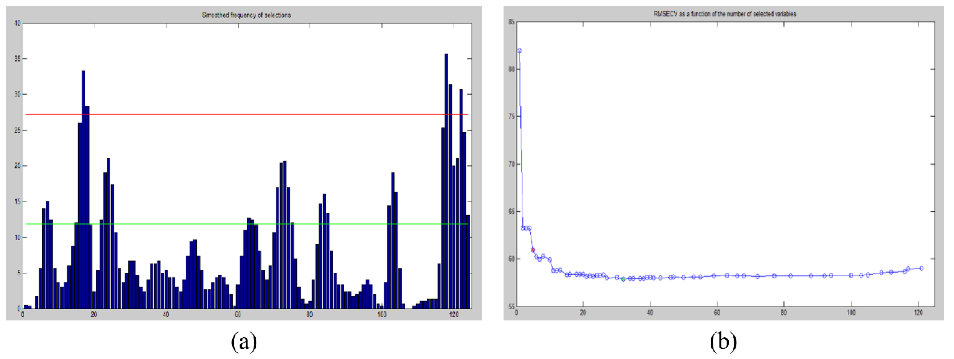
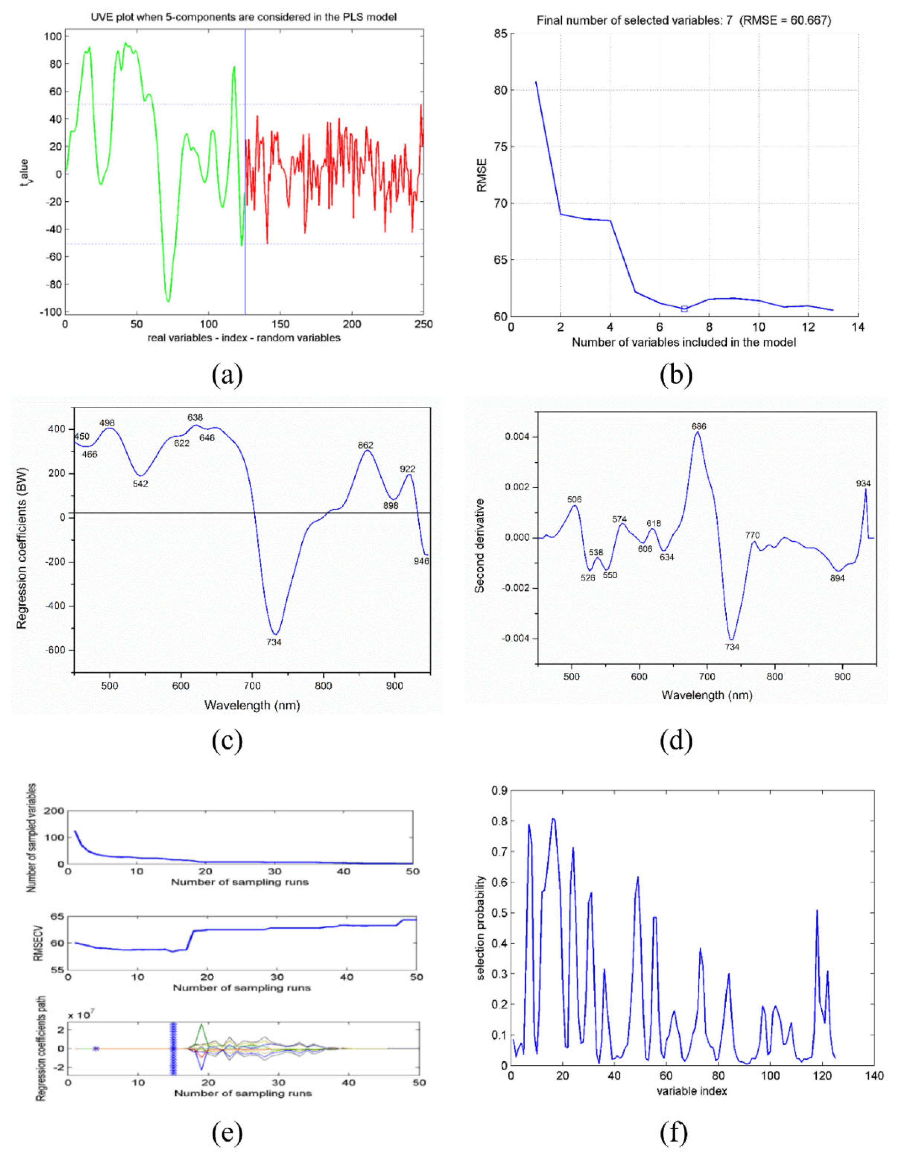
3.2. Feature Wavelength Selection and Comparison
3.3. The Yield Prediction of Oilseed Rape Based on the Effective Wavelength
3.4. Optimal Narrow-Band Vegetation Index Selection and Analysis
3.5. The Yield Prediction of Oilseed Rape Based on the Vegetation Index
4. Discussion
5. Conclusions
Supplementary Materials
Author Contributions
Funding
Institutional Review Board Statement
Data Availability Statement
Conflicts of Interest
Abbreviations
| UAV | unmanned aerial vehicle |
| EWs | effective wavelengths |
| VIs | vegetation indices |
| MLR | multiple linear regression |
| PLSR | partial least squares regression |
| ELM | extreme learning machine |
| LS-SVM | least squares support vector machine |
| CARS-ELM | competitive adaptive reweighted sampling-extreme learning machine |
| DN | digital number |
| SG | Savitzky–Golay smoothing |
| MAS | moving average smoothing |
| SNV | standard normalized variate |
| MSC | multiplicative scatter correction |
| 1-Der | first derivative |
| 2-Der | second derivative |
| WT | wavelet transform |
| SPA | successive projection algorithms |
| BW | weighted regression coefficient |
| GAPLS | genetic algorithm partial least squares |
| GA | genetic algorithm |
| UVE | uninformative variable elimination |
| CARS | competitive adaptive reweighted sampling |
| RF | random frog |
| PLS | partial least squares |
| LV | latent variable |
| SVM | support vector machine |
| R | correlation coefficient |
| RMSE | root mean square error |
| SNV-Detrending | standard normalized variable detrending |
| CV | cross-validation |
| ANOVA | one-way analysis of variance |
References
- Chen, X.; Lütken, H.; Liang, K.; Liu, F.; Favero, B.T. Superior osmotic stress tolerance in oilseed rape transformed with wild-type Rhizobium rhizogenes. Plant Cell Rep. 2024, 43, 1–12. [Google Scholar] [CrossRef] [PubMed]
- Kortesniemi, M.; Vuorinen, A.L.; Sinkkonen, J.; Yang, B.; Rajala, A.; Kallio, H. NMR metabolomics of ripened and developing oilseed rape (Brassica napus) and turnip rape (Brassica rapa). Food Chem. 2015, 172, 63–70. [Google Scholar] [CrossRef] [PubMed]
- Msanne, J.; Kim, H.; Cahoon, E.B. Biotechnology tools and applications for development of oilseed crops with healthy vegetable oils. Biochimie 2020, 178, 4–14. [Google Scholar] [CrossRef]
- Yong, K.J.; Wu, T.Y. Second-generation bioenergy from oilseed crop residues: Recent technologies, techno-economic assessments and policies. Energy Convers. Manag. 2022, 267, 115869. [Google Scholar] [CrossRef]
- Maes, W.H.; Steppe, K. Perspectives for Remote Sensing with Unmanned Aerial Vehicles in Precision Agriculture. Trends Plant Sci. 2019, 24, 152–164. [Google Scholar] [CrossRef]
- Overgaard, S.I.; Isaksson, T.; Kvaal, K.; Korsaeth, A. Comparisons of two hand-held, multispectral field radiometers and a hyperspectral airborne imager in terms of predicting spring wheat grain yield and quality by means of powered partial least squares regression. J. Near Infrared Spectrosc. 2010, 18, 247–261. [Google Scholar] [CrossRef]
- Swain, K.C.; Thomson, S.J.; Jayasuriya, H.P. Adoption of an unmanned helicopter for low-altitude remote sensing to estimate yield and total biomass of a rice crop. Trans. ASABE 2010, 53, 21–27. [Google Scholar] [CrossRef]
- Sunoj, S.; Yeh, B.; Marcaida, M., III; Longchamps, L.; van Aardt, J.; Ketterings, Q.M. Maize grain and silage yield prediction of commercial fields using high-resolution UAS imagery. Biosyst. Eng. 2023, 235, 137–149. [Google Scholar] [CrossRef]
- Verger, A.; Vigneau, N.; Cheron, C.; Gilliot, J.M.; Comar, A.; Baret, F. Green area index from an unmanned aerial system over wheat and rapeseed crops. Remote Sens. Environ. 2014, 152, 654–664. [Google Scholar] [CrossRef]
- Zhang, C.H.; Kovacs, J.M. The application of small unmanned aerial systems for precision agriculture: A review. Precis. Agric. 2012, 13, 693–712. [Google Scholar] [CrossRef]
- Ninomiya, S. High-throughput field crop phenotyping: Current status and challenges. Breed. Sci. 2022, 72, 3–18. [Google Scholar] [CrossRef] [PubMed]
- Araus, J.L.; Cairns, J.E. Field high-throughput phenotyping: The new crop breeding frontier. Trends Plant Sci. 2014, 19, 52–61. [Google Scholar] [CrossRef]
- López-García, P.; Ortega, J.F.; Pérez-Álvarez, E.P.; Moreno, M.A.; Ramírez, J.M.; Intrigliolo, D.S.; Ballesteros, R. Yield estimations in a vineyard based on high-resolution spatial imagery acquired by a UAV. Biosyst. Eng. 2022, 224, 227–245. [Google Scholar] [CrossRef]
- Adao, T.; Hruska, J.; Padua, L.; Bessa, J.; Peres, E.; Morais, R.; Sousa, J.J. Hyperspectral Imaging: A Review on UAV-Based Sensors, Data Processing and Applications for Agriculture and Forestry. Remote Sens. 2017, 9, 110. [Google Scholar] [CrossRef]
- Hassan, M.A.; Yang, M.; Rasheed, A.; Yang, G.; Reynolds, M.; Xia, X.; He, Z. A rapid monitoring of NDVI across the wheat growth cycle for grain yield prediction using a multi-spectral UAV platform. Plant Sci. 2019, 282, 95–103. [Google Scholar] [CrossRef]
- Kyratzis, A.C.; Skarlatos, D.P.; Menexes, G.C.; Vamvakousis, V.F.; Katsiotis, A. Assessment of Vegetation Indices Derived by UAV Imagery for Durum Wheat Phenotyping under a Water Limited and Heat Stressed Mediterranean Environment. Front. Plant Sci. 2017, 8, 1114. [Google Scholar] [CrossRef]
- Yu, N.; Li, L.J.; Schmitz, N.; Tiaz, L.F.; Greenberg, J.A.; Diers, B.W. Development of methods to improve soybean yield estimation and predict plant maturity with an unmanned aerial vehicle based platform. Remote Sens. Environ. 2016, 187, 91–101. [Google Scholar] [CrossRef]
- Dhillon, R.; Takoo, G.; Sharma, V.; Nagle, M. Utilizing Machine Learning Framework to Evaluate the Effect of Climate Change on Maize and Soybean Yield. Comput. Electron. Agric. 2024, 221, 108982. [Google Scholar] [CrossRef]
- Tmušić, G.; Manfreda, S.; Aasen, H.; James, M.R.; Gonçalves, G.; Ben-Dor, E.; Brook, A.; Polinova, M.; Arranz, J.J.; Mészáros, J.; et al. Current Practices in UAS-based Environmental Monitoring. Remote Sens. 2020, 12, 1001. [Google Scholar] [CrossRef]
- Bazzo, C.O.G.; Kamali, B.; Hütt, C.; Bareth, G.; Gaiser, T. A review of estimation methods for aboveground biomass in grasslands using UAV. Remote Sens. 2023, 15, 639. [Google Scholar] [CrossRef]
- Savitzky, A.; Golay, M.J. Smoothing and differentiation of data by simplified least squares procedures. Anal. Chem. 1964, 36, 1627–1639. [Google Scholar] [CrossRef]
- Barnes, R.; Dhanoa, M.S.; Lister, S.J. Standard normal variate transformation and de-trending of near-infrared diffuse reflectance spectra. Appl. Spectrosc. 1989, 43, 772–777. [Google Scholar] [CrossRef]
- Helland, I.S.; Næs, T.; Isaksson, T. Related versions of the multiplicative scatter correction method for preprocessing spectroscopic data. Chemom. Intell. Lab. Syst. 1995, 29, 233–241. [Google Scholar] [CrossRef]
- Norris, K.; Williams, P. Optimization of mathematical treatments of raw near-infrared signal in the. Cereal Chem. 1984, 61, 158–165. [Google Scholar]
- Subasi, A.; Ahmed, A.; Alickovic, E.; Hassan, A.R. Effect of photic stimulation for migraine detection using random forest and discrete wavelet transform. Biomed. Signal Process. Control 2019, 49, 231–239. [Google Scholar] [CrossRef]
- Zhu, H.; Chu, B.; Fan, Y.; Tao, X.; Yin, W.; He, Y. Hyperspectral imaging for predicting the internal quality of kiwifruits based on variable selection algorithms and chemometric models. Sci. Rep. 2017, 7, 7845. [Google Scholar] [CrossRef]
- Zhu, H.Y.; Chu, B.Q.; Zhang, C.; Liu, F.; Jiang, L.J.; He, Y. Hyperspectral Imaging for Presymptomatic Detection of Tobacco Disease with Successive Projections Algorithm and Machine-learning Classifiers. Sci. Rep. 2017, 7, 4125. [Google Scholar] [CrossRef]
- Xie, C.; Shao, Y.; Li, X.; He, Y. Detection of early blight and late blight diseases on tomato leaves using hyperspectral imaging. Sci. Rep. 2015, 5, 16564. [Google Scholar] [CrossRef]
- ElMasry, G.; Sun, D.W.; Allen, P. Near-infrared hyperspectral imaging for predicting colour, pH and tenderness of fresh beef. J. Food Eng. 2012, 110, 127–140. [Google Scholar] [CrossRef]
- Kamruzzaman, M.; ElMasry, G.; Sun, D.W.; Allen, P. Prediction of some quality attributes of lamb meat using near-infrared hyperspectral imaging and multivariate analysis. Anal. Chim. Acta 2012, 714, 57–67. [Google Scholar] [CrossRef]
- Leardi, R. Application of genetic algorithm–PLS for feature selection in spectral data sets. J. Chemom. 2000, 14, 643–655. [Google Scholar] [CrossRef]
- Han, Q.J.; Wu, H.L.; Cai, C.B.; Xu, L.; Yu, R.Q. An ensemble of Monte Carlo uninformative variable elimination for wavelength selection. Anal. Chim. Acta 2008, 612, 121–125. [Google Scholar] [CrossRef] [PubMed]
- Ye, S.; Wang, D.; Min, S. Successive projections algorithm combined with uninformative variable elimination for spectral variable selection. Chemom. Intell. Lab. Syst. 2008, 91, 194–199. [Google Scholar] [CrossRef]
- Li, H.; Liang, Y.; Xu, Q.; Cao, D. Key wavelengths screening using competitive adaptive reweighted sampling method for multivariate calibration. Anal. Chim. Acta 2009, 648, 77–84. [Google Scholar] [CrossRef]
- Li, H.D.; Xu, Q.S.; Liang, Y.Z. Random frog: An efficient reversible jump Markov Chain Monte Carlo-like approach for variable selection with applications to gene selection and disease classification. Anal. Chim. Acta 2012, 740, 20–26. [Google Scholar] [CrossRef]
- Zarco-Tejada, P.J.; Gonzalez-Dugo, V.; Berni, J.A.J. Fluorescence, temperature and narrow-band indices acquired from a UAV platform for water stress detection using a micro-hyperspectral imager and a thermal camera. Remote Sens. Environ. 2012, 117, 322–337. [Google Scholar] [CrossRef]
- Ma, L.; Li, M.C.; Ma, X.X.; Cheng, L.; Du, P.J.; Liu, Y.X. A review of supervised object-based land-cover image classification. Isprs J. Photogramm. Remote Sens. 2017, 130, 277–293. [Google Scholar] [CrossRef]
- Singh, A.; Ganapathysubramanian, B.; Singh, A.K.; Sarkar, S. Machine Learning for High-Throughput Stress Phenotyping in Plants. Trends Plant Sci. 2016, 21, 110–124. [Google Scholar] [CrossRef]
- Wu, D.; Sun, D.W. Advanced applications of hyperspectral imaging technology for food quality and safety analysis and assessment: A review—Part I: Fundamentals. Innov. Food Sci. Emerg. Technol. 2013, 19, 1–14. [Google Scholar] [CrossRef]
- Ding, S.F.; Zhao, H.; Zhang, Y.N.; Xu, X.Z.; Nie, R. Extreme learning machine: Algorithm, theory and applications. Artif. Intell. Rev. 2015, 44, 103–115. [Google Scholar] [CrossRef]
- Wang, J.; Lu, S.; Wang, S.H.; Zhang, Y.D. A review on extreme learning machine. Multimed. Tools Appl. 2022, 81, 41611–41660. [Google Scholar] [CrossRef]
- Raccuglia, P.; Elbert, K.C.; Adler, P.D.; Falk, C.; Wenny, M.B.; Mollo, A.; Norquist, A.J. Machine-learning-assisted materials discovery using failed experiments. Nature 2016, 533, 73–76. [Google Scholar] [CrossRef] [PubMed]
- Zhang, F.; O’Donnell, L.J. Support vector regression. In Machine Learning; Academic Press: Cambridge, MA, USA, 2020; pp. 123–140. [Google Scholar] [CrossRef]
- Weber, V.S.; Araus, J.L.; Cairns, J.E.; Sanchez, C.; Melchinger, A.E.; Orsini, E. Prediction of grain yield using reflectance spectra of canopy and leaves in maize plants grown under different water regimes. Field Crops Res. 2012, 128, 82–90. [Google Scholar] [CrossRef]
- Liu, D.; Sun, D.W.; Zeng, X.A. Recent Advances in Wavelength Selection Techniques for Hyperspectral Image Processing in the Food Industry. Food Bioprocess Technol. 2014, 7, 307–323. [Google Scholar] [CrossRef]
- Hansen, P.M.; Schjoerring, J.K. Reflectance measurement of canopy biomass and nitrogen status in wheat crops using normalized difference vegetation indices and partial least squares regression. Remote Sens. Environ. 2003, 86, 542–553. [Google Scholar] [CrossRef]
- Blackburn, G.A. Spectral indices for estimating photosynthetic pigment concentrations: A test using senescent tree leaves. Int. J. Remote Sens. 1998, 19, 657–675. [Google Scholar] [CrossRef]
- Broge, N.H.; Leblanc, E. Comparing prediction power and stability of broadband and hyperspectral vegetation indices for estimation of green leaf area index and canopy chlorophyll density. Remote Sens. Environ. 2001, 76, 156–172. [Google Scholar] [CrossRef]
- Carter, G.A. Ratios of leaf reflectances in narrow wavebands as indicators of plant stress. Remote Sens. 1994, 15, 697–703. [Google Scholar] [CrossRef]
- Chen, J.M. Evaluation of vegetation indices and a modified simple ratio for boreal applications. Can. J. Remote Sens. 1996, 22, 229–242. [Google Scholar] [CrossRef]
- Dash, J.; Curran, P.J. The MERIS terrestrial chlorophyll index. Int. J. Remote Sens. 2004, 25, 5403–5413. [Google Scholar] [CrossRef]
- Datt, B. Remote sensing of water content in Eucalyptus leaves. Aust. J. Bot. 1999, 47, 909–923. [Google Scholar] [CrossRef]
- Daughtry, C.S.; Walthall, C.L.; Kim, M.S.; De Colstoun, E.B.; McMurtrey Iii, J.E. Estimating corn leaf chlorophyll concentration from leaf and canopy reflectance. Remote Sens. Environ. 2000, 74, 229–239. [Google Scholar] [CrossRef]
- Diker, K.; Bausch, W.C. Potential use of nitrogen reflectance index to estimate plant parameters and yield of maize. Biosyst. Eng. 2003, 85, 437–447. [Google Scholar] [CrossRef]
- Gamon, J.A.; Penuelas, J.; Field, C.B. A narrow-waveband spectral index that tracks diurnal changes in photosynthetic efficiency. Remote Sens. Environ. 1992, 41, 35–44. [Google Scholar] [CrossRef]
- Gitelson, A.A.; Kaufman, Y.J.; Merzlyak, M.N. Use of a green channel in remote sensing of global vegetation from EOS-MODIS. Remote Sens. Environ. 1996, 58, 289–298. [Google Scholar] [CrossRef]
- Gitelson, A.A.; Zur, Y.; Chivkunova, O.B.; Merzlyak, M.N. Assessing carotenoid content in plant leaves with reflectance spectroscopy. Photochem. Photobiol. 2002, 75, 272–281. [Google Scholar] [CrossRef]
- Haboudane, D.; Miller, J.R.; Tremblay, N.; Zarco-Tejada, P.J.; Dextraze, L. Integrated narrow-band vegetation indices for prediction of crop chlorophyll content for application to precision agriculture. Remote Sens. Environ. 2002, 81, 416–426. [Google Scholar] [CrossRef]
- Haboudane, D.; Miller, J.R.; Pattey, E.; Zarco-Tejada, P.J.; Strachan, I.B. Hyperspectral vegetation indices and novel algorithms for predicting green LAI of crop canopies: Modeling and validation in the context of precision agriculture. Remote Sens. Environ. 2004, 90, 337–352. [Google Scholar] [CrossRef]
- Hernández-Clemente, R.; Navarro-Cerrillo, R.M.; Suárez, L.; Morales, F.; Zarco-Tejada, P.J. Assessing structural effects on PRI for stress detection in conifer forests. Remote Sens. Environ. 2011, 115, 2360–2375. [Google Scholar] [CrossRef]
- Huete, A.R. A soil-adjusted vegetation index (SAVI). Remote Sens. Environ. 1988, 25, 295–309. [Google Scholar] [CrossRef]
- Huete, A.; Didan, K.; Miura, T.; Rodriguez, E.P.; Gao, X.; Ferreira, L.G. Overview of the radiometric and biophysical performance of the MODIS vegetation indices. Remote Sens. Environ. 2002, 83, 195–213. [Google Scholar] [CrossRef]
- Inoue, Y.; Sakaiya, E.; Zhu, Y.; Takahashi, W. Diagnostic mapping of canopy nitrogen content in rice based on hyperspectral measurements. Remote Sens. Environ. 2012, 126, 210–221. [Google Scholar] [CrossRef]
- Jiang, Z.; Huete, A.R.; Didan, K.; Miura, T. Development of a two-band enhanced vegetation index without a blue band. Remote Sens. Environ. 2008, 112, 3833–3845. [Google Scholar] [CrossRef]
- Jordan, C.F. Derivation of leaf-area index from quality of light on the forest floor. Ecology 1969, 50, 663–666. [Google Scholar] [CrossRef]
- Kaufman, Y.J.; Tanre, D. Strategy for direct and indirect methods for correcting the aerosol effect on remote sensing: From AVHRR to EOS-MODIS. Remote Sens. Environ. 1996, 55, 65–79. [Google Scholar] [CrossRef]
- Kim, M.S.; Daughtry, C.; Chappelle, E.; McMurtrey, J.; Walthall, C. The use of high spectral resolution bands for estimating absorbed photosynthetically active radiation (A par). In CNES, Proceedings of the 6th International Symposium on Physical Measurements and Signatures in Remote Sensing, Val D’Isere, France, 1 January 1994; NASA: Washington, DC, USA, 1994; No. GSFC-E-DAA-TN72921. [Google Scholar]
- Maccioni, A.; Agati, G.; Mazzinghi, P. New vegetation indices for remote measurement of chlorophylls based on leaf directional reflectance spectra. J. Photochem. Photobiol. B Biol. 2001, 61, 52–61. [Google Scholar] [CrossRef]
- Mahlein, A.K.; Rumpf, T.; Welke, P.; Dehne, H.W.; Plümer, L.; Steiner, U.; Oerke, E.C. Development of spectral indices for detecting and identifying plant diseases. Remote Sens. Environ. 2013, 128, 21–30. [Google Scholar] [CrossRef]
- Merton, R. Monitoring community hysteresis using spectral shift analysis and the red-edge vegetation stress index. In Proceedings of the Seventh Annual JPL Airborne Earth Science Workshop, Pasadena, CA, USA, 12–16 January 1998; pp. 12–16. [Google Scholar]
- Pearson, R.L.; Miller, L.D. Remote mapping of standing crop biomass for estimation of the productivity of the shortgrass prairie, Pawnee National Grasslands, Colorado. In Proceedings of the Eighth International Symposium on Remote Sensing of Environment, Ann Arbor, MI, USA, 2–6 October 1972. [Google Scholar]
- Peñuelas, J.; Gamon, J.; Fredeen, A.; Merino, J.; Field, C. Reflectance indices associated with physiological changes in nitrogen-and water-limited sunflower leaves. Remote Sens. Environ. 1994, 48, 135–146. [Google Scholar] [CrossRef]
- Peñuelas, J.; Filella, I.; Lloret, P.; Mun Oz, F.; Vilajeliu, M. Reflectance assessment of mite effects on apple trees. Int. J. Remote Sens. 1995, 16, 2727–2733. [Google Scholar] [CrossRef]
- Qi, J.; Chehbouni, A.; Huete, A.R.; Kerr, Y.H.; Sorooshian, S. A modified soil adjusted vegetation index. Remote Sens. Environ. 1994, 48, 119–126. [Google Scholar] [CrossRef]
- Rouse, J.W.; Haas, R.H.; Schell, J.A.; Deering, D.W. Monitoring vegetation systems in the Great Plains with ERTS. NASA Spec. Publ 1974, 351, 309. [Google Scholar]
- Rondeaux, G.; Steven, M.; Baret, F. Optimization of soil-adjusted vegetation indices. Remote Sens. Environ. 1996, 55, 95–107. [Google Scholar] [CrossRef]
- Roujean, J.-L.; Breon, F.-M. Estimating PAR absorbed by vegetation from bidirectional reflectance measurements. Remote Sens. Environ. 1995, 51, 375–384. [Google Scholar] [CrossRef]
- Sims, D.A.; Gamon, J.A. Relationships between leaf pigment content and spectral reflectance across a wide range of species, leaf structures and developmental stages. Remote Sens. Environ. 2002, 81, 337–354. [Google Scholar] [CrossRef]
- Vogelmann, J.E.; Rock, B.N.; Moss, D.M. Red edge spectral measurements from sugar maple leaves. Remote Sens. 1993, 14, 1563–1575. [Google Scholar] [CrossRef]
- Wu, C.; Niu, Z.; Tang, Q.; Huang, W. Estimating chlorophyll content from hyperspectral vegetation indices: Modeling and validation. Agric. For. Meteorol. 2008, 148, 1230–1241. [Google Scholar] [CrossRef]
- Zarco-Tejada, P.J.; Miller, J.R.; Noland, T.L.; Mohammed, G.H.; Sampson, P.H. Scaling-up and model inversion methods with narrowband optical indices for chlorophyll content estimation in closed forest canopies with hyperspectral data. IEEE Trans. Geosci. Remote Sens. 2001, 39, 1491–1507. [Google Scholar] [CrossRef]
- Zarco-Tejada, P.J.; Berjón, A.; Lopez-Lozano, R.; Miller, J.R.; Martín, P.; Cachorro, V.; De Frutos, A. Assessing vineyard condition with hyperspectral indices: Leaf and canopy reflectance simulation in a row-structured discontinuous canopy. Remote Sens. Environ. 2005, 99, 271–287. [Google Scholar] [CrossRef]
- Zarco-Tejada, P.J.; Berni, J.A.; Suárez, L.; Sepulcre-Cantó, G.; Morales, F.; Miller, J.R. Imaging chlorophyll fluorescence with an airborne narrow-band multispectral camera for vegetation stress detection. Remote Sens. Environ. 2009, 113, 1262–1275. [Google Scholar] [CrossRef]


| Sample Sets | Number | Minimum (kg/hm2) | Maximum (kg/hm2) | Mean (kg/hm2) | Median (kg/hm2) | Standard Deviation (SD) | Coefficient of Variation (%) | Kurtosis | Skewness |
|---|---|---|---|---|---|---|---|---|---|
| Calibration | 248 | 2217.3 | 3586.3 | 2942.68 | 2977.70 | 274.23 | 9.31 | −0.41 | −0.37 |
| Prediction | 125 | 2217.3 | 3526.8 | 2947.24 | 3023.80 | 292.97 | 9.94 | −0.20 | −0.53 |
| Preprocessing Method | Models | LVs | Calibration | Prediction | ||
|---|---|---|---|---|---|---|
| Rcal | RMSEC | Rpre | RMSEP | |||
| - | PLSR | 4 | 0.7771 | 172.3 | 0.7770 | 183.8 |
| MAS | PLSR | 4 | 0.7750 | 173.0 | 0.7733 | 207.4 |
| SG | PLSR | 4 | 0.7768 | 172.4 | 0.7771 | 183.8 |
| MSC | PLSR | 5 | 0.7178 | 190.5 | 0.6365 | 225.5 |
| SNV | PLSR | 9 | 0.7182 | 190.4 | 0.6384 | 225.1 |
| SNV-Detrending | PLSR | 9 | 0.7141 | 191.6 | 0.6122 | 231.5 |
| 1-Der | PLSR | 5 | 0.7144 | 191.5 | 0.6722 | 216.1 |
| 2-Der | PLSR | 2 | 0.6430 | 209.6 | 0.5026 | 257.1 |
| WT | PLSR | 4 | 0.7767 | 172.4 | 0.7775 | 183.6 |
| Algorithms | (No.) | Selected EWs (nm) |
|---|---|---|
| SPA | 7 | 858, 474, 746, 638, 510, 554, and 910 |
| GAPLS | 32 | 918, 514, 922, 934, 518, 510, 914, 938, 542, 930, 738, 734, 926, 538, 858, 546, 730, 742, 862, 782, 474, 778, 854, 470, 786, 942, 698, 478, 534, 702, 506, and 746 |
| UVE | 52 | 486–522, 582–754, 914–922, and 938 |
| UVE-SPA | 7 | 730, 494, 486, 650, 914, 754, and 938 |
| BW | 12 | 450, 466, 498, 542, 622, 638, 646, 734, 862, 898, 922, and 946 |
| 2-Der | 13 | 506, 526, 538, 550, 574, 606, 618, 634, 686, 734, 770, 894, and 934 |
| CARS | 8 | 478, 498, 506, 542, 598, 914, 918, and 922 |
| RF | 29 | 510, 514, 474, 478, 506, 542, 518, 502, 642, 538, 498, 522, 494, 570, 638, 566, 918, 546, 666, 670, 646, 470, 738, 742, 590, 574, 634, 934, and 782 |
| Wavelength Selection Algorithms | EWs | Models | LVs/(γ, σ2)/ Hidden Neurons | Calibration | Prediction | ||
|---|---|---|---|---|---|---|---|
| Rcal | RMSEC | Rpre | RMSEP | ||||
| - | 125 | PLSR | 4 | 0.7767 | 172.4 | 0.7775 | 183.6 |
| - | 125 | MLR | - | 0.8988 | 140.1 | 0.6588 | 247.2 |
| - | 125 | LS-SVM | (76.4, 5.6 × 10³) | 0.8012 | 163.9 | 0.7703 | 186.1 |
| - | 125 | ELM | 48 | 0.8221 | 155.8 | 0.8019 | 175.2 |
| SPA | 7 | PLSR | 4 | 0.7760 | 172.6 | 0.7787 | 183.2 |
| SPA | 7 | MLR | - | 0.7805 | 171.1 | 0.7919 | 179.0 |
| SPA | 7 | LS-SVM | (127.0, 392.1) | 0.7894 | 168.0 | 0.7783 | 183.2 |
| SPA | 7 | ELM | 20 | 0.7963 | 165.5 | 0.8056 | 173.1 |
| GAPLS | 32 | PLSR | 4 | 0.7803 | 171.1 | 0.7824 | 181.9 |
| GAPLS | 32 | MLR | - | 0.7999 | 164.3 | 0.7846 | 181.0 |
| GAPLS | 32 | LS-SVM | (6.4 × 10³, 3.6 × 10⁴) | 0.7893 | 168.1 | 0.7888 | 179.4 |
| GAPLS | 32 | ELM | 39 | 0.8100 | 160.5 | 0.8060 | 172.9 |
| UVE | 52 | PLSR | 4 | 0.7793 | 171.5 | 0.7803 | 182.6 |
| UVE | 52 | MLR | - | 0.8459 | 147.3 | 0.7037 | 214.0 |
| UVE | 52 | LS-SVM | (347.2, 2.7 × 10³) | 0.8006 | 164.0 | 0.7464 | 194.4 |
| UVE | 52 | ELM | 47 | 0.8281 | 153.4 | 0.7888 | 180.2 |
| UVE-SPA | 7 | PLSR | 4 | 0.7756 | 172.8 | 0.7773 | 183.8 |
| UVE-SPA | 7 | MLR | - | 0.7816 | 170.7 | 0.7858 | 180.6 |
| UVE-SPA | 7 | LS-SVM | (9.4 × 10³, 5.1 × 10³) | 0.7895 | 168.0 | 0.7881 | 179.7 |
| UVE-SPA | 7 | ELM | 29 | 0.8069 | 161.7 | 0.8050 | 173.4 |
| BW | 12 | PLSR | 4 | 0.7798 | 171.7 | 0.7750 | 184.5 |
| BW | 12 | MLR | - | 0.7853 | 169.8 | 0.7707 | 186.1 |
| BW | 12 | LS-SVM | (2.2 × 10³, 5.3 × 10³) | 0.7914 | 167.3 | 0.7798 | 182.7 |
| BW | 12 | ELM | 31 | 0.8101 | 160.5 | 0.7980 | 176.0 |
| 2-Der | 13 | PLSR | 4 | 0.7705 | 174.5 | 0.7694 | 186.5 |
| 2-Der | 13 | MLR | - | 0.7810 | 170.9 | 0.7594 | 189.9 |
| 2-Der | 13 | LS-SVM | (44.5, 279.1) | 0.7916 | 167.3 | 0.7453 | 194.6 |
| 2-Der | 13 | ELM | 8 | 0.7734 | 173.5 | 0.7879 | 179.9 |
| CARS | 8 | PLSR | 4 | 0.7750 | 173.0 | 0.7853 | 180.8 |
| CARS | 8 | MLR | - | 0.7844 | 169.8 | 0.7979 | 176.0 |
| CARS | 8 | LS-SVM | (381.5, 333.1) | 0.7952 | 166.0 | 0.7737 | 184.9 |
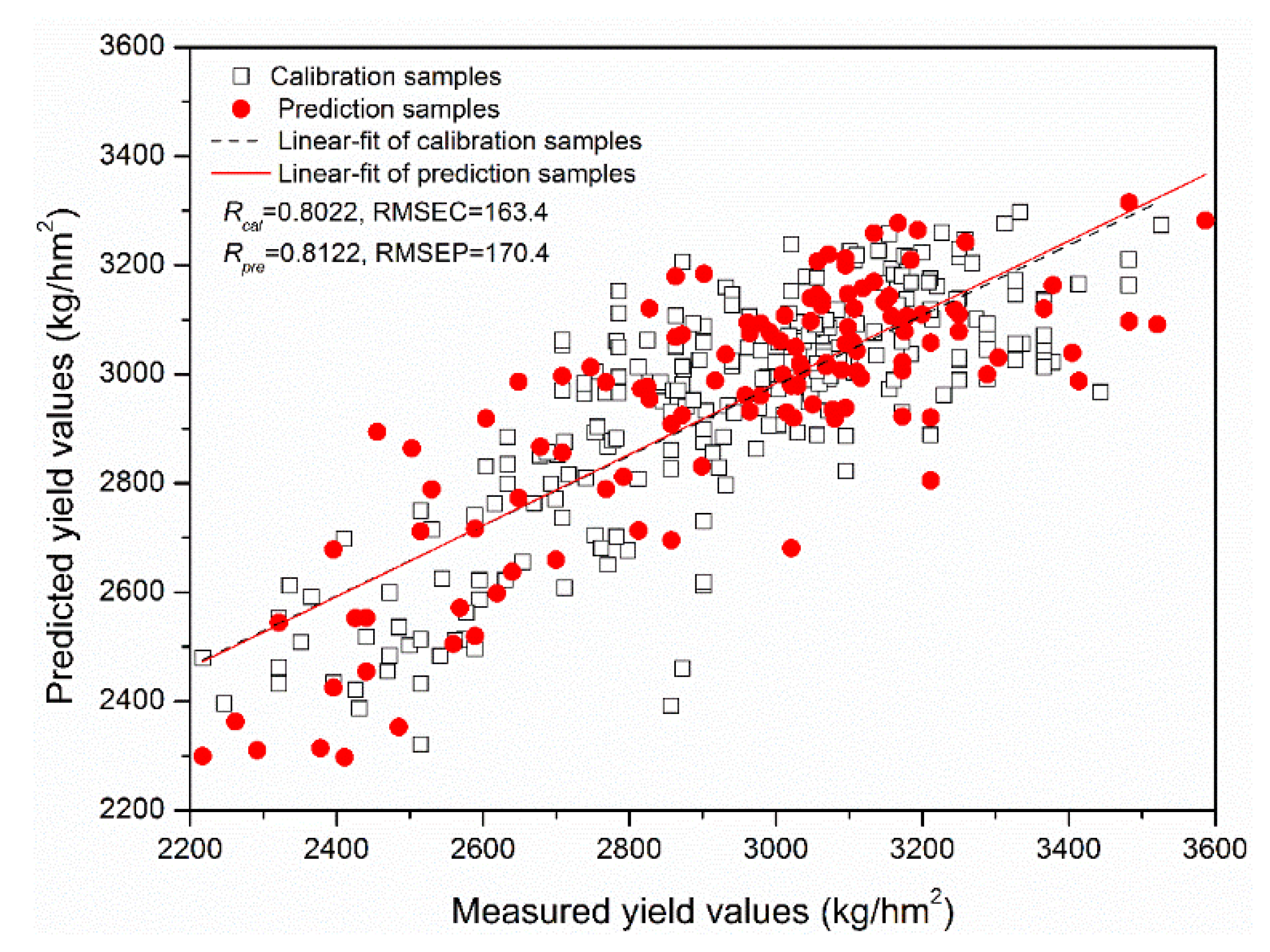
| CARS | 8 | ELM | 21 | 0.8022 | 163.4 | 0.8122 | 170.3 |
| RF | 29 | PLSR | 4 | 0.7792 | 171.5 | 0.7906 | 179.0 |
| RF | 29 | MLR | - | 0.8136 | 160.5 | 0.7743 | 186.2 |
| RF | 29 | LS-SVM | (2.1 × 10³, 2.8 × 10³) | 0.8078 | 161.4 | 0.7746 | 184.6 |
| RF | 29 | ELM | 39 | 0.8224 | 155.7 | 0.8018 | 175.0 |
| (No.) | Models | LVs/(γ, σ2)/ Hidden Neurons | Calibration | Prediction | ||
|---|---|---|---|---|---|---|
| Rcal | RMSEC | Rpre | RMSEP | |||
| 14 | PLSR | 2 | 0.7605 | 177.7 | 0.7736 | 185.4 |
| 14 | MLR | - | 0.7813 | 170.8 | 0.7670 | 187.4 |
| 14 | LS-SVM | (0.80, 72.2) | 0.7952 | 166.3 | 0.7493 | 193.5 |
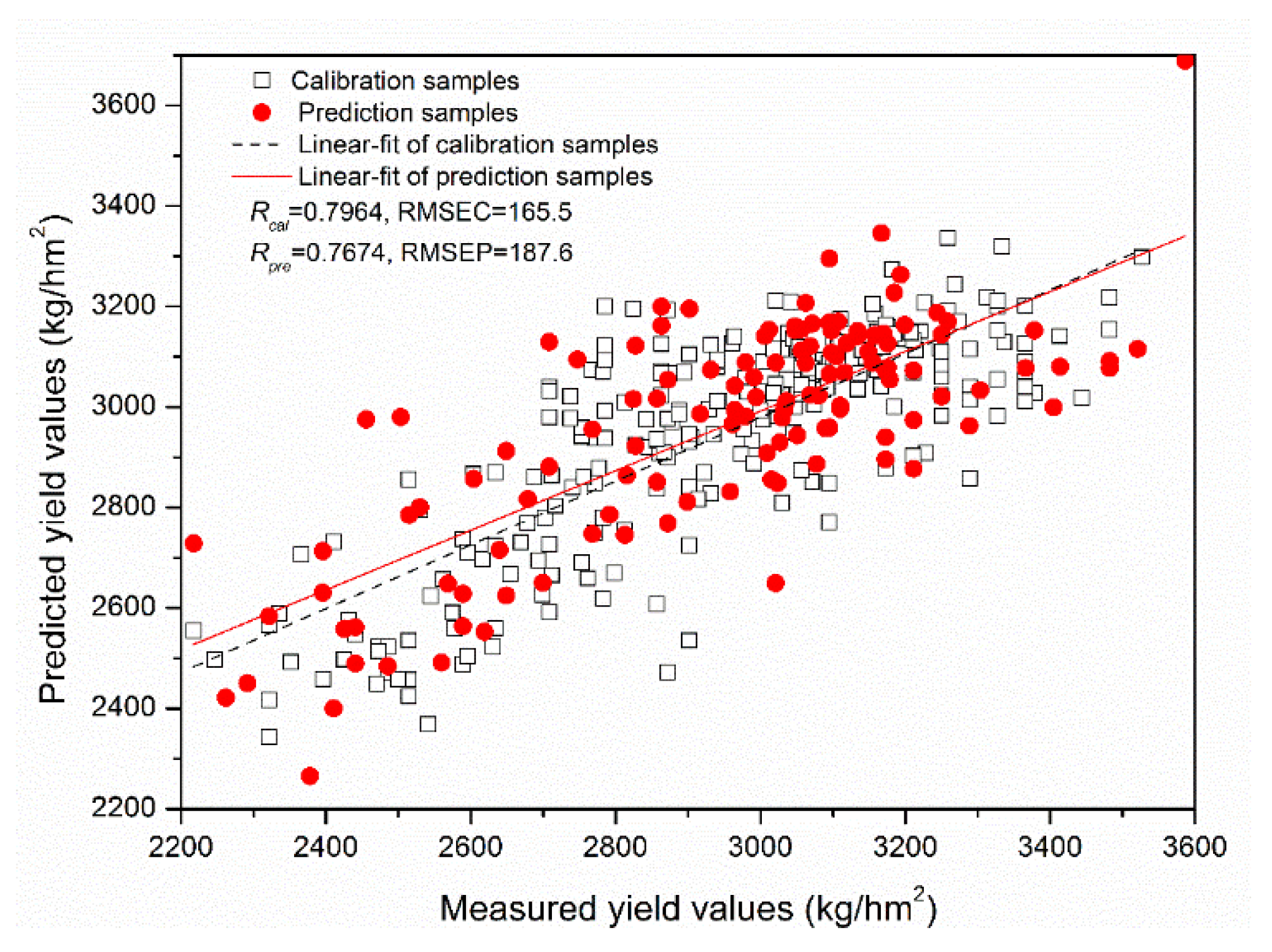
| 14 | ELM | 27 | 0.7964 | 165.5 | 0.7674 | 187.6 |
Disclaimer/Publisher’s Note: The statements, opinions and data contained in all publications are solely those of the individual author(s) and contributor(s) and not of MDPI and/or the editor(s). MDPI and/or the editor(s) disclaim responsibility for any injury to people or property resulting from any ideas, methods, instructions or products referred to in the content. |
© 2025 by the authors. Licensee MDPI, Basel, Switzerland. This article is an open access article distributed under the terms and conditions of the Creative Commons Attribution (CC BY) license (https://creativecommons.org/licenses/by/4.0/).
Share and Cite
Zhu, H.; Lin, C.; Dong, Z.; Xu, J.-L.; He, Y. Early Yield Prediction of Oilseed Rape Using UAV-Based Hyperspectral Imaging Combined with Machine Learning Algorithms. Agriculture 2025, 15, 1100. https://doi.org/10.3390/agriculture15101100
Zhu H, Lin C, Dong Z, Xu J-L, He Y. Early Yield Prediction of Oilseed Rape Using UAV-Based Hyperspectral Imaging Combined with Machine Learning Algorithms. Agriculture. 2025; 15(10):1100. https://doi.org/10.3390/agriculture15101100
Chicago/Turabian StyleZhu, Hongyan, Chengzhi Lin, Zhihao Dong, Jun-Li Xu, and Yong He. 2025. "Early Yield Prediction of Oilseed Rape Using UAV-Based Hyperspectral Imaging Combined with Machine Learning Algorithms" Agriculture 15, no. 10: 1100. https://doi.org/10.3390/agriculture15101100
APA StyleZhu, H., Lin, C., Dong, Z., Xu, J.-L., & He, Y. (2025). Early Yield Prediction of Oilseed Rape Using UAV-Based Hyperspectral Imaging Combined with Machine Learning Algorithms. Agriculture, 15(10), 1100. https://doi.org/10.3390/agriculture15101100