Article

Hyperspectral Estimation of Tea Leaf Chlorophyll Content Based on Stacking Models

1
College of Resources and Environment, Yili Normal University, Yining 835000, China
2
Institute of Resources and Ecology, Yili Normal University, Yining 835000, China
3
College of Ecology and Environment, Baotou Teachers’ College, Baotou 014030, China
4
School of Geographic Sciences, East China Normal University, Shanghai 200241, China
*
Author to whom correspondence should be addressed.
Agriculture 2025, 15(10), 1039; https://doi.org/10.3390/agriculture15101039
Submission received: 15 March 2025 / Revised: 4 May 2025 / Accepted: 7 May 2025 / Published: 11 May 2025
(This article belongs to the Section Digital Agriculture)

Abstract

:
Chlorophyll is an essential pigment for photosynthesis in tea plants, and fluctuations in its content directly impact the growth and developmental processes of tea trees, thereby influencing the final quality of the tea. Therefore, achieving rapid and non-destructive real-time monitoring of leaf chlorophyll content (LCC) is beneficial for precise management in tea plantations. In this study, derivative transformations were first applied to preprocess the tea hyperspectral data, followed by the use of the Stable Competitive Adaptive Reweighted Sampling (SCARS) algorithm for feature variable selection. Finally, multiple individual machine learning models and stacking models were constructed to estimate tea LCC based on hyperspectral data, with a particular emphasis on analyzing how the selection of base models and meta-models affects the predictive performance of the stacking models. The results indicate that derivative processing enhances the sensitivity of hyperspectral data to tea LCC; furthermore, compared with individual machine learning models, the stacking models demonstrate superior predictive accuracy and generalization ability. Among the 17 constructed stacking configurations, when the meta-model is fixed, the predictive performance of the stacking model improves continuously with an increase in the number and accuracy of the base models and with a decrease in the structural similarity among the selected base models. Therefore, when constructing stacking models, the base model combination should comprise various models with minimal structural similarity while ensuring robust predictive performance, and the meta-model should be chosen as a simple linear or nonlinear model.

1. Introduction

Chlorophyll is a vital pigment for plant photosynthesis, helping plants convert solar energy into chemical energy [1]. Changes in chlorophyll content in tea leaves can affect the photosynthesis of the tea tree, thereby influencing its growth and development. In addition, the chlorophyll content in tea leaves is closely related to the content of an important chemical component—catechins [2]. In summary, as a crucial pigment in tea trees, the chlorophyll content in tea leaves not only reflects the photosynthetic capacity and growth stage of the tree but also has a critical impact on the final tea quality [3,4,5]. Accurate and timely monitoring of chlorophyll content in tea leaves is advantageous for implementing precision management strategies in tea plantation operations. Traditional laboratory chemical analysis methods are time-consuming, labor-intensive, and highly destructive, making them unsuitable for real-time, large-scale monitoring in the field [6]. Remote sensing technology, a prime example of non-destructive monitoring, enables the rapid assessment of plant physiological and biochemical parameters using spectral reflectance and vegetation index data [7,8]. With the ongoing advancement of remote sensing in agriculture, its application for real-time, accurate, and rapid monitoring of LCC in crops at various scales (including ground, aerial, and satellite remote sensing) has become a significant driver of precision agriculture [8,9,10].
Although hyperspectral data provide rich spectral information, adjacent bands often show high correlation and redundancy. Additionally, noise signals, sample humidity, and experimental conditions during data acquisition can degrade the quality of hyperspectral data [11]. Therefore, employing various preprocessing methods to extract meaningful spectral information from a large number of spectral bands is essential for subsequent modeling [12]. To minimize the influence of external factors, common preprocessing techniques include Savitzky–Golay (S-G) smoothing, mathematical transformations, derivative transformations (first-order derivative (FD), second-order derivative (SD)), standard normal variate (SNV), wavelet transform (WT), and multiplicative scatter correction (MSC). Each of these methods offers distinct advantages, such as smoothing spectra, eliminating instrumental errors, reducing noise, and enhancing weak spectral features. He et al. found that hyperspectral data processed with FD, SNC, and S-G exhibited higher signal-to-noise ratios than raw spectral data from similar samples [13]. Jin et al., in their study of tracking canopy transpiration in desert plants, found that the derivative spectral index was more effective than the original reflectance index for tracking canopy transpiration [14]. This further highlights the critical role of spectral data preprocessing in enhancing the effectiveness of hyperspectral analysis. Spectral derivatives, a widely used preprocessing method, effectively eliminate baseline drift, reduce noise, enhance weak spectral features, and remove spectral overlaps [15]. Zhang et al. applied the CR, MSC, and SD algorithms to preprocess hyperspectral data of apple leaves and found that the CatBoost model built using SD preprocessing exhibited the best predictive performance [16]. Similarly, Zhou et al. employed SG, SNV, MSC, FD, and SD preprocessing methods for hyperspectral data of lettuce leaves and discovered that the modeling accuracy was highest for the data preprocessed with FD and SD [17]. These studies demonstrate the advantages of derivative transformations in enhancing the predictive performance of hyperspectral data.
Variable selection algorithm, as a key step in modeling hyperspectral data, reduces the redundancy of hyperspectral data and improves the prediction performance of the model by eliminating useless spectral information and filtering the characteristic bands [18,19]. Yun et al.’s study also proves the importance of variable selection algorithms in the complex analysis system [20]. In the past, random forest (RF), successive projection algorithm (SPA), variable combination cluster analysis (VCPA), CARS, and other algorithms have been widely used for dimensionality reduction of hyperspectral data, in which the CARS algorithm can adaptively reweight and select spectral bands by simulating the process of “biological evolution”, eliminating redundant and unimportant bands. It also shows better robustness while having better stability [21,22,23,24]. Chen et al. compared the two variable selection algorithms of CARS and RF, and found that the CARS algorithm has a unique advantage in retaining effective spectral features and reducing modeling redundancy [25]. Li et al. investigated modeling results based on SPA, CARS, SiPLS, and SiPLS-SPA, and found that the CARS algorithm provided the highest modeling accuracy when used to extract sensitive spectral bands [26]. These findings underscore the distinct advantage of the CARS algorithm in processing hyperspectral data. In addition, Tan et al. applied the CARS algorithm to airborne hyperspectral data and successfully constructed an inversion model for soil heavy metal content [27]. By comprehensively considering the stability of the selected variables, Zheng et al. proposed the SCARS algorithm based on the CARS algorithm. By comparing the SCARS algorithm with the selected variables of CARS, MCUVE, and MWPLS, they found that SCARS provides the smallest RMSECV and the smallest number of potential variables while selecting the fewest variables [28]. Jiang et al.’s research shows that compared with the CARS algorithm, the PLS-DA model based on the SCARS algorithm to select wavelength variables has the best accuracy [29].
Recent years have witnessed notable advancements in constructing predictive regression frameworks. Among traditional machine learning models, PLSR and SVM are key representatives of linear and nonlinear models, respectively. Both models exhibit strong generalization ability and robustness and offer distinct advantages when dealing with high-dimensional data and small sample sizes [30,31]. For example, Subi et al. found that the PLSR model outperformed others in predicting Cr concentration in farmland in arid areas [32]. With the ongoing development of machine learning algorithms, a variety of models, such as the ELM, GBDT, GPR, RF, XGBoost, BPNN, and LSTM, have been widely used in studies on plant parameters, soil parameters, and healthcare due to their strong data mining and fitting capabilities [8,27,33]. For example, Yue et al. observed in their research on estimating crop leaf area index and chlorophyll content that the LACNet deep learning model showed significantly better predictive performance compared to traditional machine learning models [34]. Sudu et al.’s study showed that the DNN model outperformed traditional models such as PLSR, SVM, and XGBoost in predicting maize SAPD values [35]. In recent years, GA, PSO, and ACO have been applied to optimize machine learning model parameters, enhancing their global search ability and prediction performance. Chang et al. implemented the DPSO algorithm for parameter optimization in BPNN architectures, demonstrating that this hybrid computational framework exhibits superior operational consistency and predictive accuracy compared to traditional approaches [36]. Wang et al. combined GA with machine learning models and successfully improved prediction performance [37].
When using a single machine learning model, its predictive performance is often limited by the model’s inherent structure, and it is highly susceptible to overfitting, particularly when processing small sample sizes [38,39,40]. In the study of crop parameters, Huang et al. improved the model’s predictive performance by generating training data using physical models [41]. Among various machine learning models, ensemble learning methods such as bagging, boosting, and stacking enhance predictive performance by leveraging the diversity of results from multiple models [42,43]. For example, Lin et al. demonstrated that combining the AdaBoost algorithm with machine learning models can significantly improve model stability and accuracy [42]. In contrast to bagging and boosting, which construct the training set by sampling or combining multiple similar models iteratively, the stacking model introduces a two-layer structure consisting of a base model and a meta-model [44]. In the first layer, multiple machine learning models are used to train the dataset and generate predictions [45,46]. In the second layer, the outputs of these base models are combined as inputs for the meta-model, which produces the final predictions [47]. This unique two-tier structure makes stacking a powerful solution to the limitations of single machine learning models and helps reduce overfitting. For instance, studies such as Tan et al. prove the advantages of the stacking model in improving model prediction performance and reducing model overfitting ability [27]. In addition, studies by Yao and Huang et al. have shown that the predictive accuracy of stacking models based on a dual-layer model structure outperforms that of individual machine learning models [41,48].
Although the stack model has been widely used in the inversion of soil and plant physicochemical properties [41,49], crop seed variety discrimination [50], water quality index prediction [51], etc., few scholars have estimated tea chlorophyll content based on the stack model. In this study, derivative transformations were applied to preprocess the hyperspectral data of tea leaves, followed by the use of the SCARS algorithm to extract sensitive spectral bands. Multiple machine learning models were then constructed. By conducting comparative analyses between the stacked ensemble framework and standalone machine learning models, we comprehensively evaluated the potential of stacked modeling in alleviating overfitting issues while simultaneously boosting prediction accuracy. Moreover, through rigorous assessment of stacked models built with varying base model configurations and meta-model architectures, we study how these factors affect the overall performance of stacked models.

2. Materials and Methods

2.1. Experimental Design

The research site is situated in the Chahui Tea Garden, located in Xihu District, Hangzhou City, Zhejiang Province (120°04′–120°10′ E, 30°10′–30°16′ N). This area experiences a characteristic subtropical monsoon climate, featuring a mean yearly temperature that spans 17 °C to 18 °C. The region receives 1300–1600 mm of yearly rainfall, with the majority (78.6%) concentrated during summer cultivation periods. Geographically, the area is characterized by low mountains and hills, with higher elevations in the western and central parts, resulting in a relatively complex terrain. The main soil types in the tea gardens of Xihu District are yellow clay soil and white sandy soil, with soil pH values ranging from 4.6 to 5.0, which is highly suitable for tea tree growth. To ensure the representativeness of the experimental data both temporally and spatially, sampling was carried out in April 2021, during the peak growing season of the tea trees, when the average daily temperature had stabilized above 15 °C for 10 consecutive days. All samples were immediately sealed in polyethylene self-sealing bags, which had been sterilized beforehand, and properly stored in a temperature-controlled box to maintain their stability. The spatial arrangement of the sampling points is depicted in Figure 1.

2.2. HYPERSPECTRAL Data Measurement and Pre-Processing

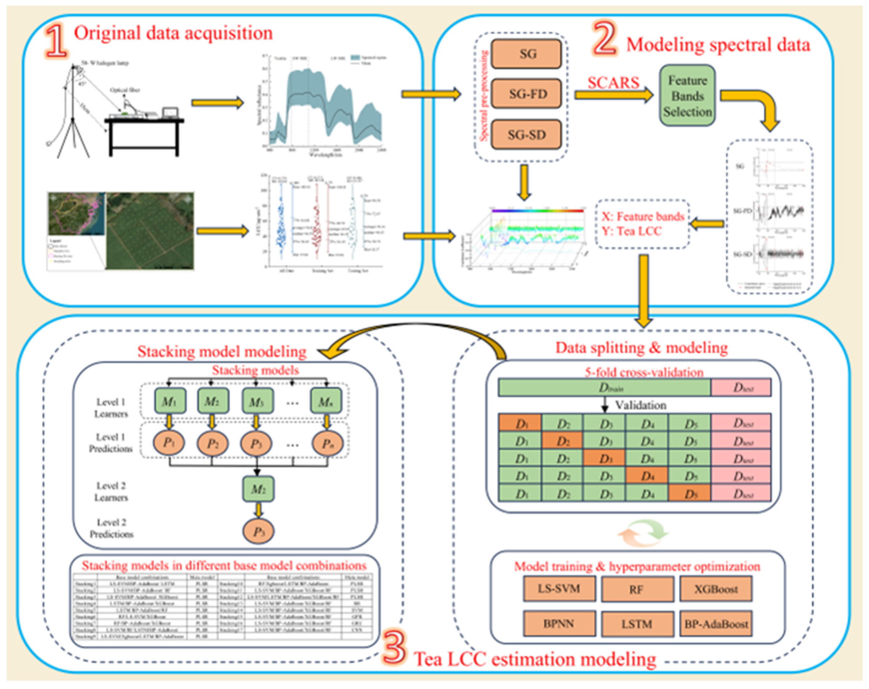
The hyperspectral reflectance of tea leaves was measured using a portable field spectroradiometer ASD FieldSpec 3® Hi-Res (Analytical Spectral Devices, Inc., Boulder, CO, USA), which covers a spectral range of 350–2500 nm. To minimize the interference of ambient light, the measurements were conducted in a darkroom, as shown in Figure 2. A 50 W halogen lamp was set at a zenith angle of 45° and positioned 35 cm from the sample. The optical probe was adjusted using a bracket so that it was located 3 cm directly above the sample stage, with a field of view of 25°. Each sample was measured 10 times, and the average spectral reflectance was taken as the final reflectance value. A white reference calibration was performed before each measurement. To reduce the impact of noise on hyperspectral data in the future, we removed the 350–399 nm and 2401–2500 nm spectral bands, and then applied the Savitzky–Golay (S-G) filter to the remaining hyperspectral data [8,52], which was considered as the original hyperspectral data. Furthermore, to further reduce noise and enhance weak spectral features, derivative transformation methods in Origin 2022 were applied, utilizing first- and second-order derivatives to process the original hyperspectral data.

2.3. LCC Measurement

The LCC was determined using laboratory chemical analysis methods. First, a hole puncher (diameter: 0.846 cm) was used to punch holes on one side of the leaf, avoiding the veins. The punched sections were subsequently sliced into smaller fragments using scissors and transferred into stoppered test tubes. Next, 10 mL of 80% acetone solution was added, and the tubes were kept in the dark. They were shaken several times until the leaf tissues turned white, after which the absorbance of the supernatant at 646.8 nm and 663.2 nm was measured using a UV-6100 UV–visible spectrophotometer (Shanghai Yuanxi Instruments Co., Ltd., Shanghai, China). Finally, the chlorophyll content of the tea leaves was calculated according to Equations (1) and (2) [53].
C a + b = 18.71 A 646.8 + 7.15 A 663.2
C = C a + b V 1000 S
where C a + b is the total chlorophyll concentration in the extract (mg/L), A 646 and A 663 are the absorbance values of chloroplast pigments at 646 nm and 663 nm, respectively, C is the chloroplast pigment content (µg/cm2), V is the volume of the extract (L), and S is the area of the leaf (cm2).

2.4. Variable Selection Algorithm

The Stability Competitive Adaptive Reweighted Sampling (SCARS) algorithm is an improved version of the CARS algorithm. It incorporates variable stability considerations to enhance the robustness of selected features and improve the model’s prediction accuracy [29]. The SCARS algorithm initially constructs a PLS model by randomly choosing a subset of samples from the calibration set using Monte Carlo sampling. It then calculates the stability of variables across spectral bands. Subsequently, Forced Band Selection and Adaptive Reweighted Sampling (ARS) techniques are employed to select spectral features based on variable stability. The selected variables are retained as a subset for use in the next iteration. After completing all iterations, multiple variable subsets are generated, and the Monte Carlo RMSECV of the PLS model is computed. The band combination yielding the smallest RMSECV value is identified as the optimal configuration.

2.5. Constructing Models

2.5.1. LS-SVM

LS-SVM, an improved version of SVM, uses a least squares linear system as the loss function, solving a set of linear equations rather than the complex quadratic optimization problem in the traditional SVM [54]. Consequently, LS-SVM operates significantly faster than SVM. When applying LS-SVM, it is essential to choose an appropriate kernel function. The polynomial kernel function is commonly used with LS-SVM because it can find the decision boundary in high-dimensional space without explicitly calculating the coordinates in that space, thus effectively handling nonlinear problems. The general form of the polynomial kernel function is:
k ( x , y ) = ( x · y + c ) d
where x and y are two input vectors, c is a constant term, and d is the degree (or power) of the polynomial kernel function. By adjusting the parameters c and d, the complexity of the polynomial kernel in the feature space can be controlled to better suit different datasets and problems. In this study, we set the constant term c = 1 and the degree of the polynomial kernel d = 3.

2.5.2. RF

Random forest (RF) is an ensemble algorithm based on a collection of decision trees [55]. It is known for its simplicity, fast computation, and low computational overhead. The RF algorithm begins by using a bootstrap method to randomly draw K samples from the full dataset. Each time, the number of samples drawn matches the number of trees in the forest, resulting in K training subsets. For each sample, a random subset of features is also selected. These randomly selected subsets and their corresponding feature subsets are then used to construct classification or regression trees, which together form a forest. For the regression trees, the average predicted value of all trees is computed. In this study, the number of decision trees is set to 100, with the minimum number of observations per leaf (cotyledons) set to 5.

2.5.3. XGBoost

The XGBoost model is a typical ensemble algorithm [56]. It builds a strong predictive model by successively training multiple weak models (decision trees). In each iteration, XGBoost optimizes the model by minimizing the gradient of the objective function. Specifically, it trains a new classifier in each iteration based on the error from the previous round of predictions. The predictions from these classifiers are weighted and combined to form the final output of the model. The XGBoost model was configured with 100 boosting iterations, a learning rate of 0.1, a maximum tree depth of 5, an L1 regularization coefficient (α) of 0.1, and an L2 regularization coefficient (λ) of 1.0.

2.5.4. LSTM

LSTM (Long Short-Term Memory) is a type of recurrent neural network (RNN) designed to address the issues of gradient vanishing and gradient explosion in traditional RNN structures. It effectively controls the flow of information through a gating mechanism [57]. The LSTM model consists of three components: the input layer, the output layer, and the hidden layers, where the hidden layers contain multiple LSTM units. Each LSTM unit has three gates: the input gate, the forget gate, and the output gate. These gates manage the inflow, retention, and outflow of information through logical operations, enabling the capture of long-term dependencies in sequential data. Set the maximum number of training iterations to 500, the initial learning rate to 0.01, the learning rate decay factor to 0.1, and the regularization parameter to 1 × 10⁻⁴.

2.5.5. BPNN

The backpropagation neural network (BPNN) effectively models arbitrary non-linear mappings from input to output by continuously adjusting the weights and thresholds through backpropagation [58]. This process minimizes network error, and the learning results are then fed back to the hidden layer to update the weight coefficient matrix, thereby achieving the desired learning outcome. Set the number of iterations to 1000, the learning rate to 0.01, and the error threshold to 1 × 10⁻⁶. The selection of the number of hidden layers is calculated using an empirical formula [59], as shown in Equation (4):
y = a + b + c
In the equation, y represents the number of neurons in the hidden layer; a represents the number of neurons in the input layer; b represents the number of neurons in the output layer; and c is an integer from 1 to 10.

2.5.6. BP-AdaBoost

The BP-AdaBoost algorithm is an ensemble learning method that combines BP neural networks with AdaBoost techniques to construct a strong regression model by using multiple BP neural networks as weak regressors [60]. Initially, each sample is assigned an equal weight to balance its effect on the model. Through iterative training, each iteration is based on the prediction error of the previous iteration, optimizing the overall model’s performance. This approach helps reduce the overfitting issue of the BP neural network in regression tasks and enhances the model’s ability to predict new data. Ultimately, the predictions of all weak regressors are weighted and combined to form the final output of the model. In this study, the number of weak regressors is set to 10, the number of iterations is 1000, and the learning rate is 0.01. In this study, the number of hidden layers is determined using Equation (4), the number of weak regressors is set to 10, the number of iterations is 1000, and the learning rate is set to 0.01.

2.5.7. PLSR

Partial Least Squares Regression (PLSR) combines dimensionality reduction with regression modeling by projecting the independent variables into latent components that maximize covariance with the response variable [27]. This approach effectively handles multicollinearity while enhancing both prediction accuracy and model stability. In the current study, the optimal number of latent components was determined to be 3 through cross-validation.

2.5.8. RR

Ridge Regression is an enhanced linear regression algorithm developed to address multicollinearity (high correlation between features) in the data. It increases the reliability of the regression coefficients by compromising the unbiasedness of the least squares method [61]. In this study, the regularization parameter of RR is set to 0.1.

2.5.9. SVM

Support Vector Machine Regression (SVMR), a typical nonlinear model, transforms the original features into a higher-dimensional space using a kernel function [62]. Different kernel functions can lead to different modeling results. In this study, the RBF is employed for modeling.

2.5.10. GPR

Gaussian Process Regression (GPR) is a typical non-parametric regression model. It is trained using past data to update the prior distribution, transforming it into a posterior model that generates statistically significant predictions [63].

2.5.11. GRU

The Gated Recurrent Unit (GRU) is a variation of the Recurrent Neural Network (RNN) developed for processing sequential data [64]. It is designed such that the network’s output from the previous time step serves as the input for the current time step through connections between the nodes in the hidden layer. This structure allows the GRU to capture long-term dependencies better. Set the maximum number of iterations to 1000, the initial learning rate to 0.01, and the regularization parameter to 1 × 10⁻⁴.

2.5.12. CNN

Convolutional Neural Network (CNN) is a deep learning model that utilizes a feed-forward neural network structure with convolutional computation and a multi-layer architecture [65]. The basic components of a CNN include the input layer, convolutional layer, activation layer, pooling layer, and fully connected layer. When processing spectral data, the convolutional layer automatically extracts feature bands. After convolution, a bias is typically added, followed by a nonlinear activation function, which produces the final prediction result. Set the number of iterations to 1000, the initial learning rate to 0.001, and the regularization parameter to 1 × 10⁻³.

2.5.13. Stacking Model

The stacking model, a typical ensemble algorithm, is usually constructed as a two-level learning network. The first level consists of multiple base models, and the second level consists of a meta-model [66]. In this approach, the prediction results from each base model on the first level are used as input parameters for the meta-model on the second level. To achieve model diversity, base models are typically selected from different algorithms with significant differences in their principles and performance, and their parameters are optimized using cross-validation. Compared with a single machine learning model, the stacking algorithm utilizes the advantages of multiple algorithms to provide better nonlinear fitting and generalization capabilities [42].
In this study, the prediction performance of LS-SVM, RF, LSTM, BPNN, BP-AdaBoost, and XGBoost models at 0th-order, 1st-order, and 2nd-order was comprehensively compared. Finally, following the requirement that base model selections maintain maximum diversity, various combinations of LS-SVM, RF, XGBoost, BP-AdaBoost, and LSTM were designated as first-level base models. To systematically investigate how meta-model selection impacts the predictive performance of stacked models, we selected two linear models (PLSR, RR), two nonlinear models (SVM, GPR), and two deep learning architectures (GRU, CNN) as candidate meta-models. In this study, both variable selection algorithms and machine learning model development were implemented using MATLAB R2024a.

2.6. Evaluation Indicators

In this study, the predictive performance of the model was evaluated using the R2, RMSE, MAE, MAPE, and RPD. The formulas for these metrics are as follows:
R 2 = 1 i = 1 n ( x i x ^ i ) 2 i = 1 n ( x i x ¯ ) 2
R M S E = i = 1 n ( x i x ^ i ) 2 n
M A E = 1 n | x i x ^ i | n
M A P E = 1 n | x i x ^ i x i | n × 100 %
R P D = S D R M S E
where n is the number of samples, x i is the ith measured LCC for each sample, x ^ i is the ith estimated LCC for each sample, x ¯ is the mean LCC, and S D is the standard deviation.

3. Results

3.1. Descriptive Statistics

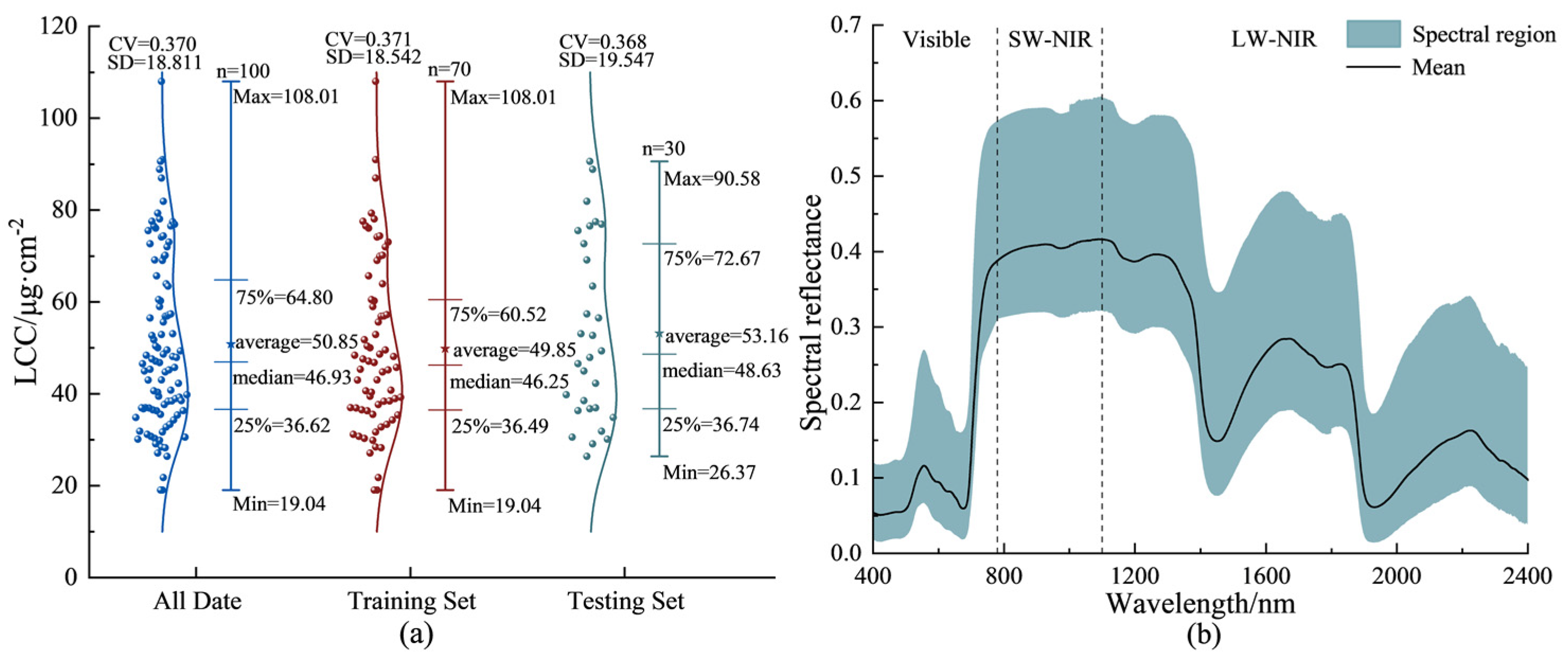
One hundred tea samples were collected for this study. Due to the small sample size, the tea leaves were reordered by their LCC values, from low to high, to improve the accuracy of model predictions. The training and test sets were then sequentially extracted in a 7:3 ratio. Descriptive statistics for both the test and training sets are presented in Figure 3a. The LCC values of the leaf samples ranged from 19.04 to 108.01 μg/cm2, with an average of 50.85 μg/cm2. The distribution ranges of LCC, coefficient of variation (CV), and standard deviation (SD) are similar for both sets, indicating that the division of the training and test sets is reasonable and suitable for subsequent training and testing.
The distribution range of leaf hyperspectral curves, along with the average hyperspectral curves, is presented in Figure 3b. Both the distribution ranges of the original hyperspectral curves and the average curves of the samples display the reflectance characteristics of typical healthy vegetation in the visible range (400–780 nm). The spectral curves of the leaf samples overlapped significantly in the 400–750 nm interval, indicating a narrower spectral range. The reflectance of tea leaves increased rapidly in the 670–750 nm range, and beyond 750 nm, the spectral reflectance varied more noticeably. Chlorophyll strongly absorbs blue and red light while reflecting green light, leading to two absorption valleys and one reflection peak in the visible range (400–780 nm). Furthermore, due to the influence of leaf water content, two additional absorption valleys are observed in the spectral curves at 1450 nm and 1950 nm.

3.2. Feature Variable Selection

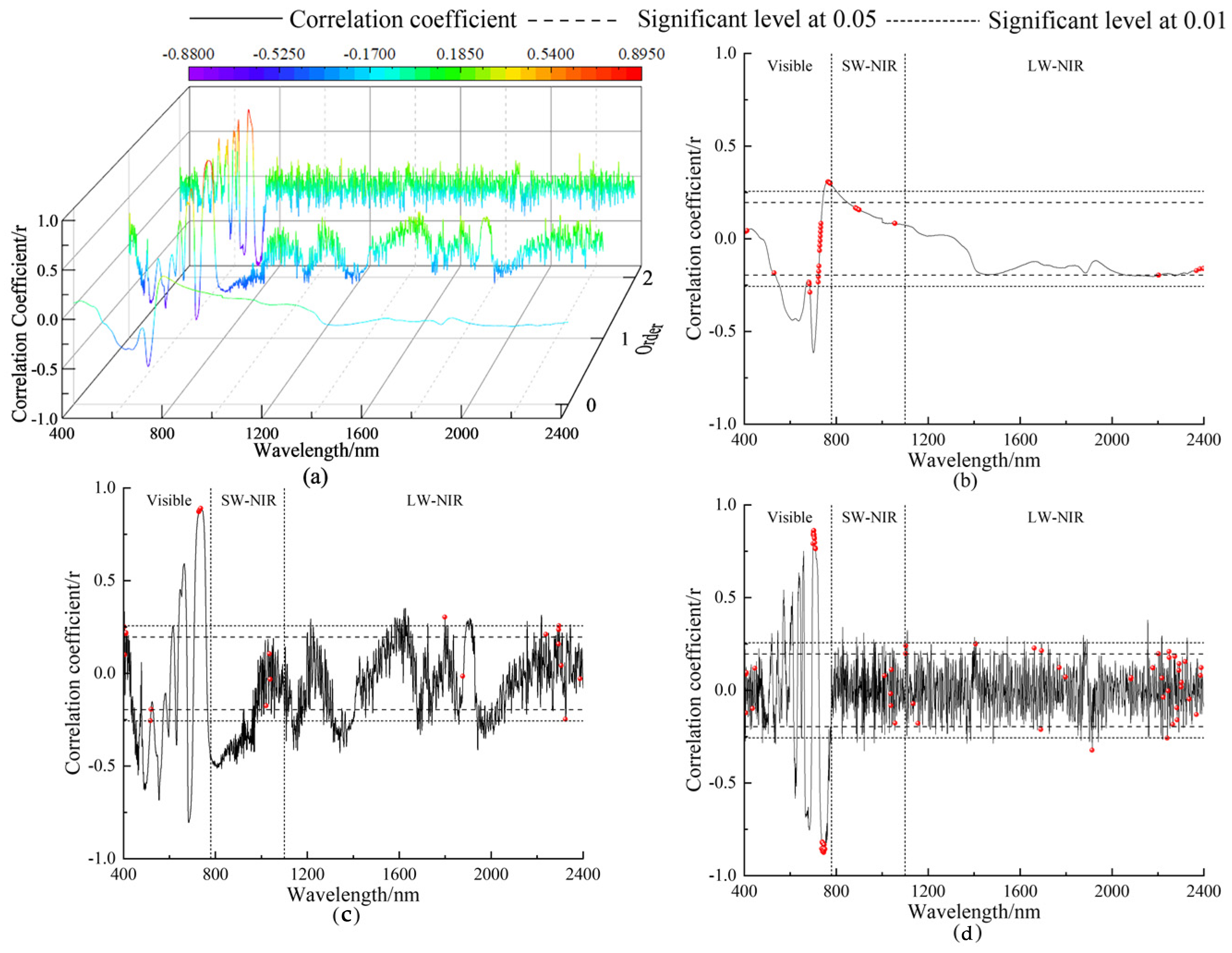
The original spectral data and the tea leaf hyperspectral dataset transformed by the 1st-order and 2nd-order derivatives were analyzed using Pearson correlation with tea LCC, where the correlation coefficient (r) ranges from −1 to 1. As shown in Figure 4a, the Pearson correlation results between the 0–2 order spectral datasets of tea leaves and the LCC are presented. Comparative analysis indicates that derivative transformation can, to some extent, enhance the sensitivity of leaf spectral data to LCC. Table 1 presents the positive and negative correlations, as well as the total number of bands, between the 0–2 order spectral datasets and the LCC based on a 0.01 correlation threshold, with R_max representing the maximum absolute value of the correlation coefficient. The number of positive, negative, and total bands after the 1st-order derivative transformation is greater than that of the 0th-order derivative transformation. For the 2nd-order derivative transformation, the total number of bands is similar to that of the 0th-order data, but the number of positive bands is larger. Notably, the correlation coefficient reaches its maximum value of 0.891 at the 736 nm band after the 1st-order derivative transformation.
To select the best modeling variables and reduce redundant information, thereby improving modeling accuracy, this study applied the SCARS algorithm to select feature variables from the 0–2 order spectral data. As shown in Figure 4b–d, the number of feature bands selected by the SCARS algorithm is 44, 22, and 68, respectively, with the increase in derivative order. The selected regions are roughly similar. By comparing and analyzing the selected band position with its correlation coefficient, it is found that the selected band in the 1st-order and 2nd-order hyperspectral data sets contains the spectrum interval with the largest correlation coefficient, except for the selected band in the original spectral data set.

3.3. Tea LCC Estimation Model

3.3.1. Tea LCC Single Model Construction

The best feature band combinations selected using the SCARS algorithm were used as input parameters for the model, with the tea LCC serving as the output parameter. Estimation models for tea LCC were then established using the LS-SVM, RF, LSTM, BPNN, BP-AdaBoost, and XGBoost algorithms. The prediction performance of the six models was uniformly evaluated using R2, RMSE, MAE, MAPE, and RPD, with the training and test set division shown in Figure 3a. As presented in Table 2, among the six regression models, the LSTM model demonstrated the best performance when the original spectral data were used as input (test set R2 = 0.903, RMSE = 5.971 µg/cm2, MAPE = 10.659%, RPD = 3.224 µg/cm2), followed by the BP-AdaBoost model (test set R2 = 0.881, MAPE = 10.899%, RPD = 2.940 µg/cm2). The RF model, however, had the lowest R2 and RPD, showing the worst performance on the test set. When spectral data with 1st-order and 2nd-order derivatives were used as input, the LSTM model with 1st-order differentiation achieved the best performance, with an R2 of 0.926 and an RPD of 4.535 on the test set, followed by the BP-AdaBoost model with 1st-order differentiation (R2 = 0.918, RMSE = 5.503 µg/cm2, MAPE = 10.478%, RPD = 3.817 µg/cm2).
The regression models for predicting tea LCC were constructed using the original spectral data, as well as the spectral data after 1st-order and 2nd-order derivative transformations. The predictive performances of the six models revealed distinct patterns. The model using the original spectral data showed the poorest performance, while the model with 1st-order derivative transformation achieved the best performance, followed by the model with 2nd-order differentiation. Comprehensive analysis of the models built using 0–2 order differentiated data shows that the LSTM model performed the best, followed by BP-AdaBoost and BPNN. The overall performance ranking of the six models is as follows: LSTM > BP-AdaBoost > BPNN > XGBoost > RF > LS-SVM. Among all the models, the LS-SVM model performed the worst, while the model built with 1st-order derivative transformation achieved the best prediction results, followed by the 2nd-order model. The LSTM model, built with 1st-order differential processing, achieved the highest R2 and RPD, as well as the lowest RMSE and MAPE. The BP-AdaBoost and BPNN models also showed strong performance, while the LS-SVM and XGBoost models exhibited slight overfitting when the original spectral data were used as input. It is noteworthy that among the six aforementioned machine learning models, the LSTM, BPNN, and BP-AdaBoost models achieved R2 values above 0.9 on some test sets. However, their MAPE still exceeded 10%, which may be due to substantial deviations in the predictions for certain samples, thereby inflating the MAPE values.

3.3.2. Stacking Integrated Learning Algorithm and Model Estimation Results

The stacking integration algorithm enhances model generalization and prediction performance by combining multiple base regression models with a meta-regression model to form a stronger overall prediction model. Considering the structure and prediction performance of the six machine learning models discussed earlier, this study constructs 12 different stacking models by using various combinations of LS-SVM, XGBoost, RF, BP-AdaBoost, and LSTM as base models, with PLSR as the meta-model. The base model combinations for the stacking algorithm are shown in Table 3. The training and test sets used for the stacking models are the same as those used for the single-model predictions.
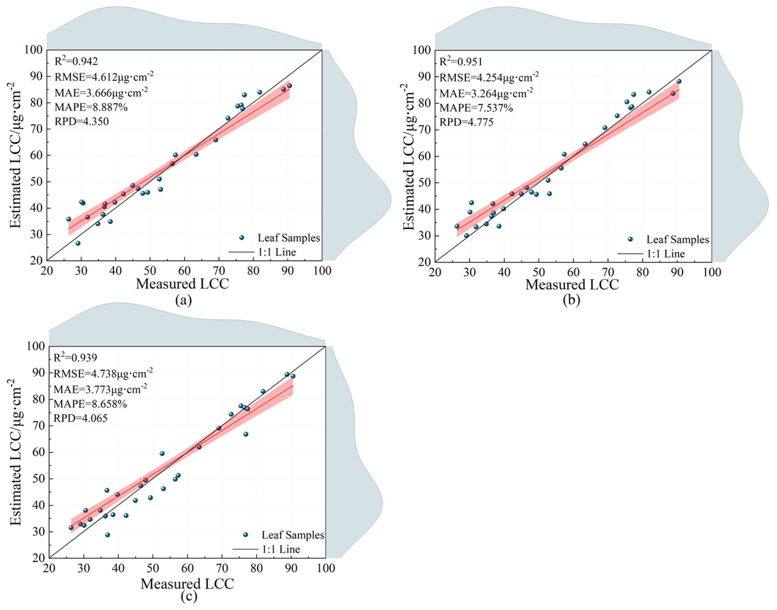
The modeling results for the stacking integrated models, constructed using 12 different combinations of base models, are shown in Table 4. The tea LCC estimation models were built using the original spectral data, as well as the spectral data processed by 1st-order and 2nd-order derivative transformations, as input parameters. Comparing Table 4 with Table 2 reveals that the models after derivative transformations generally outperform those using the original spectral data. Notably, Stacking2, built with 1st-order differentiation, achieved the best prediction performance (test set R2 = 0.951, RMSE = 4.254 µg/cm2, MAPE = 7.537%, RPD = 4.775 µg/cm2, Figure 5b), followed by Stacking8 (R2 = 0.939, RMSE = 4.738 µg/cm2, MAPE = 8.658%, RPD = 4.065 µg/cm2, Figure 5c) constructed with 2nd-order differentiation, and Stacking12 (R2 = 0.939, RMSE = 4.746 µg/cm2, MAPE = 8.831%, RPD = 4.056 µg/cm2).
When raw spectral data were used as input, the prediction performance of Stacking6 (R2 = 0.817, RMSE = 8.228 µg/cm2, MAPE = 13.621%, RPD = 2.338 µg/cm2) and Stacking10 (R2 = 0.869, RMSE = 6.963 µg/cm2, MAPE = 13.362%, RPD = 2.777 µg/cm2) was lower than some of the single-model results. However, the prediction performance of most other stacking models improved to varying degrees compared to the single models. However, the prediction performance of most other stacking models improved to varying degrees compared to the single models. Except for the lower performance of Stacking6 and Stacking10 with raw data, all 12 stacking models, constructed with different combinations of base models, achieved R2 values greater than 0.91, MAPEs below 14%, and RPDs greater than 3 µg/cm2, demonstrating strong prediction capabilities. Among them, Stacking4, built with the original spectral data, achieved the best performance (test set R2 = 0.942, RMSE = 4.612 µg/cm2, MAPE = 8.887%, RPD = 4.350 µg/cm2, Figure 5a).
By comparing the predictive performance of the models in Table 2 and Table 4, it can be observed that, compared to the LS-SVM model, the predictive performance of the 12 stacking models has improved to varying degrees over three ensemble models (RF, XGBoost, and BP-AdaBoost) and two deep learning models (BPNN and LSTM). Except for Stacking6 and Stacking10, the predictive performance of the stacking models has significantly enhanced compared to individual machine learning models. When using the original hyperspectral data as well as spectral data processed by first-order and second-order derivatives as input parameters for the models, the R2 values of the stacking models, compared to the LS-SVM model, increased by 0.262–0.288, 0.141–0.15, and 0.158–0.164, respectively; compared to the three ensemble models, the R2 values increased by 0.035–0.378, 0.024–0.06, and 0.046–0.107, respectively; compared to the two deep learning models, the R2 values increased by 0.013–0.081 and 0.016–0.043, respectively, with a larger increase of 0.024–0.124 for one model. This demonstrates the feasibility and effectiveness of the stacking models in estimating tea LCC.
By comparing and analyzing the relationship between the predictive performance of 11 ensemble models and the stacking models presented in Table 5, it was observed that when both BP-AdaBoost and LSTM models were included in the base model combination, the predictive performance of the stacking model did not exhibit a clear pattern of change as the number of base models increased. However, when the base model combination included only BP-AdaBoost or LSTM models, the predictive performance of the stacking model improved with an increasing number of base models. Nevertheless, no clear pattern was observed between the improvement in the predictive performance of the stacking model and the performance of the added base models.

3.4. Analysis of the Impact of Metamodel Selection on Stacking Models

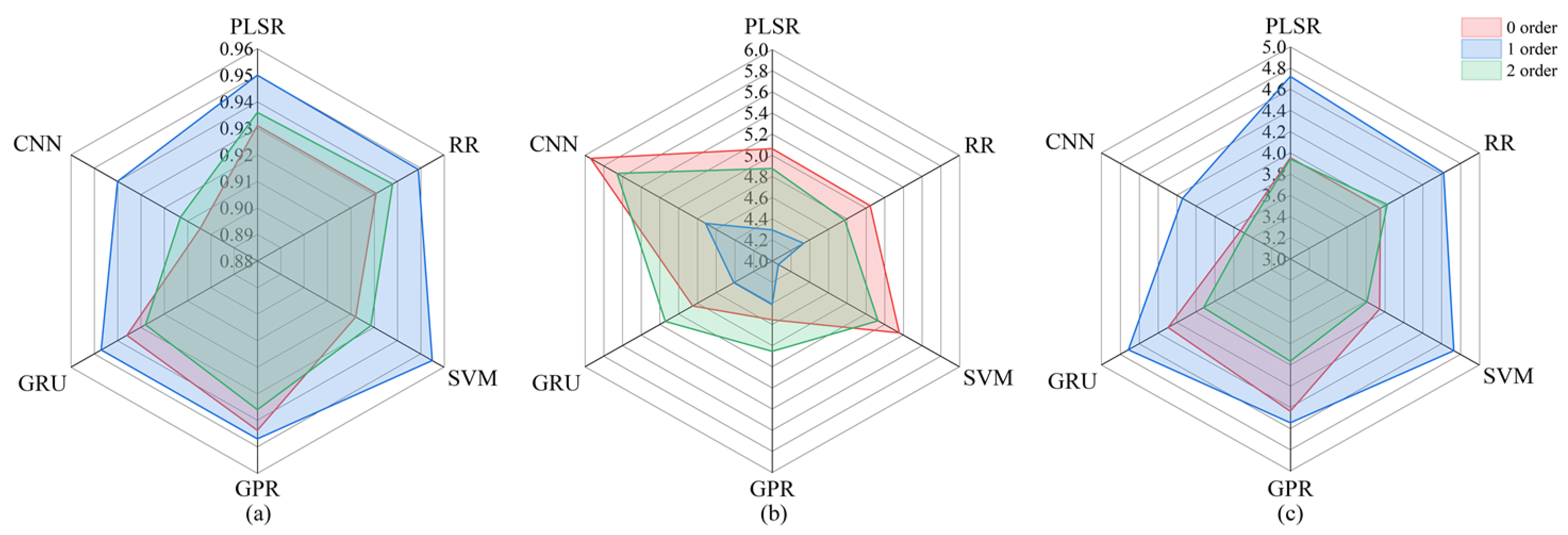
By comprehensively considering the different base model combinations in Table 3 and the predictive performance of the stacking models in Table 4, this study re-designed the base model combinations of Stacking11 for 0th, 1st, and 2nd orders based on the use of PLSR as the meta-model. RR, SVM, GPR, GRU, and CNN were selected as the meta-models, and the corresponding models Stacking13, Stacking14, Stacking15, Stacking16, and Stacking17 were constructed. The predictive performance of these models on the test set is shown in Figure 6.
When comparing and analyzing the prediction performance of stacking models constructed by six different metamodels on the test set, this study aimed to mitigate the influence of low-performing base models on metamodels. By examining the prediction performance of stacking models using spectral datasets transformed by 1st-order and 2nd-order derivatives, it was observed that Stacking11, Stacking13, Stacking14, and Stacking15 exhibited the strongest prediction performance. Among these, Stacking11 and Stacking13 demonstrated the strongest overall predictive performance. However, when constructing the Stacking14 model, it is necessary to experiment with various kernel functions to determine the optimal parameters. During the process of constructing the stacked model using CNN and GRU as base models, even after multiple tests of the model’s hyperparameters, only Stacking16 demonstrated strong predictive performance, while Stacking17 still exhibited relatively low R2 and RPD values, as well as relatively high RMSE.

4. Discussion

Leaf chlorophyll content (LCC), a key biochemical parameter in plants, shows a close relationship with leaf N content, allowing it to function as an essential indicator of nitrogen levels [67]. In addition, variations in LCC concentrations serve as a reliable indicator for evaluating vegetative development stages, nutrient assimilation efficiency, photosynthetic performance, and stress response levels in plants [8]. Hyperspectral remote sensing data, characterized by high spatial and spectral resolution and the ability for large-scale, continuous data collection, allows for rapid, non-destructive, real-time monitoring of LCC, making it a widely used tool for this purpose. To reduce the influence of external factors on hyperspectral data [68], various preprocessing methods such as mathematical transformations, wavelet transforms, integer-order differential transforms, and continuous spectral removal are applied. Among these, integer-order differential transforms are particularly effective in reducing background noise and enhancing the quality of the data. These transforms also excel at improving weak spectral features [69,70].
In this study, integer-order differentiation was applied to process the original hyperspectral data of tea leaves. As illustrated in Figure 4 and Table 1, r-values between hyperspectral measurements and LCC exhibited marked improvement following 1st-order and 2nd-order differentiation. Within the near-infrared range, derivative-processed spectra demonstrated significantly stronger associations compared to raw spectral data. As shown in Table 1, in the 0–2 order spectral datasets, the maximum correlation coefficients are all located in the red-edge region (670–760 nm). This is because variations in chlorophyll content directly influence the spectral reflectance in the red-edge region, rendering its spectral features highly sensitive to changes in chlorophyll content. When the SCARS algorithm is used to select features of 0–2 order hyperspectral data, the selected spectrum interval is similar to that of the hyperspectral feature spectrum interval extracted by Huang et al. [71] using the CARS algorithm from tomato seedling leaves chlorophyll a. This is because different spectral regions carry distinct information about chlorophyll content. In the 0–2 order spectral datasets, the SCARS algorithm selected feature intervals primarily in the green region around 520 nm, where chlorophyll absorption is minimal; the near-infrared region of 700–770 nm, which reflects both chlorophyll content and leaf structure; and the short-wave near-infrared region of 2300–2400 nm, used for monitoring plant health and water status. Notably, after derivative transformation, the absorption region around 1100 nm, associated with water molecules that indirectly indicate chlorophyll content, was also chosen as an input parameter for hyperspectral LCC estimation models.
When feature selection is performed on the 1st-order hyperspectral data set, the number of selected bands is only half of the number of selected bands on the original hyperspectral data set, but when feature selection is performed on the 2nd-order hyperspectral data set, the total number of selected feature bands and the number of selected bands in the LW-NIR range increase rapidly. As seen in Table 2 and Table 4, the regression models built with 0th-order, 1st-order, and 2nd-order spectral data show that the overall prediction performance follows the order: 1st-order > 2nd-order > 0th-order. This result is consistent with the findings of Shi et al. [72]. The reason for this phenomenon is that the 1st-order derivative transform helps balance noise reduction and preserve spectral features, while the 2nd-order derivative transform makes the data too smooth and sensitive to noise, which may reduce the signal-to-noise ratio [73].
Six machine learning algorithms were selected in this study to establish estimation models for tea LCC, with the prediction accuracies of these models shown in Table 2. By comparing two typical ensemble models (RF, XGBoost) with two deep learning models (BPNN, LSTM), it is evident that the deep learning models generally outperform the ensemble models. This finding is consistent with previous studies Chen et al. [74], Wang et al. [75] and Danner et al. [76], and may be due to the fact that deep learning models are more complex, enabling better feature learning and the ability to process high-dimensional data, which helps capture complex relationships among the input parameters. Among the three ensemble models evaluated, the BP-AdaBoost model, which combines the principles of BPNN and Boosting, outperforms RF, XGBoost, and BPNN, demonstrating the advantages of ensemble methods in improving prediction accuracy. Among the six machine learning models evaluated (LS-SVM, RF, LSTM, BPNN, BP-AdaBoost, and XGBoost), BPNN, LSTM, and BP-AdaBoost demonstrated particularly strong predictive performance; however, their hyperparameter tuning procedures proved substantially more intricate than those of LS-SVM, RF, and XGBoost, which in turn further elevated the computational cost of model training.
Among the six conventional algorithmic frameworks evaluated in this investigation, LS-SVM and XGBoost exhibited patterns analogous to Tan et al.’s findings [27], achieving perfect training set performance but reduced test set accuracy, demonstrating pronounced overfitting under limited sample size conditions. This is due to the certainty of model structure, incorrect feature selection, and small sample size in a single machine learning model can reduce predictive performance [27,77]. As a representative ensemble architecture, the stacking algorithm incorporates a meta-learner within its hierarchical framework, synthesizing the strengths of diverse base learners to enhance generalization capacity and predictive accuracy [78,79]. The comparative analysis across Table 2 and Table 4 demonstrates that all 12 stacked architectures maintain overfitting-free performance while surpassing standalone algorithmic approaches in predictive accuracy, thereby confirming the viability of stacked generalization for tea leaf chlorophyll content (LCC) estimation. Unlike the stacking model established by Du et al. [77], this study incorporates deep learning models into part of the base model combinations. Specifically, the stacking integrated model was constructed with 12 different base model combinations, using PLSR as the meta-model. The regression prediction model for LCC was built using the 0–2 order spectral dataset selected by SCARS as the input. By comparing and analyzing Stacking1–7, it can be seen that when the base model combination in the stacking model includes high-performing models such as LSTM or BP-AdaBoost, the predictive performance of the stacking model is far superior to that of stacking models constructed with lower-performing base models like LS-SVM, RF, and XGBoost. Moreover, stacking models built using first-order spectral data outperform those constructed with 0th- and 2nd-order data. This demonstrates that the predictive performance of the base models can significantly affect that of the stacking model.
Furthermore, a comparison of Stacking8–11 reveals that when both LSTM and BP-AdaBoost models are included in the base model combination, the predictive performance of the stacking model is lower than that of Stacking11. In addition, the comparative analysis between Table 4 and Table 5 shows that when both BP-AdaBoost and LSTM models are included in the base model combination, the stacking model’s predictive performance does not exhibit a clear trend with an increasing number of base models, which contradicts the findings of Du et al. [77]. In contrast, when the base model combination consistently includes only BP-AdaBoost or LSTM models, the change in the stacking model’s predictive performance aligns with the results reported by Du et al. [77]. A comprehensive analysis suggests that this may be because when the base model combination contains only one deep learning model, its structural differences with other machine learning algorithms are maximized, thereby enhancing the overall predictive performance. Even though the BPNN is optimized through ensemble algorithms, its model structure, regarding hierarchy, learning process, and error propagation, is similar to that of LSTM. When base learners exhibit similar architectural configurations, the meta-learner’s capacity to capture output feature representations becomes constrained, thereby limiting the ensemble system’s predictive effectiveness and resulting in diminished prediction accuracy. The study indicates that the predictive performance of the stacking model depends not only on the performance of the base models but also on the structure and number of base models used in the ensemble.
By employing two linear regression models (PLSR, RR), two nonlinear regression models (SVM, GPR), and two deep learning models (GRU, CNN) as meta-models, and constructing stacking models with the same base models in various combinations, the analysis of the modeling process and the final results reveals that parameter tuning is necessary when developing meta-models. Moreover, this tuning becomes increasingly complex with higher complexity of the meta-model structures. Additionally, the stability of the stacking model’s predictions tends to diminish as the complexity of the meta-models escalates. Specifically, both the stability and overall predictive performance of the stacking model’s forecasts decline progressively when the meta-models are selected in the order of linear, nonlinear, and deep learning models. Furthermore, excessive model complexity can lead to overfitting, potentially due to the fact that the input parameters for the meta-models are the output parameters of the base models. When the model structure becomes overly complex, it may enhance the interdependence among models, thereby reducing the model’s predictive performance.
In summary, the predictive performance of the stacking model is not solely determined by the performance of the base models. When constructing an ensemble model, the selection of base learning model combinations should ensure both high predictive performance and significant structural diversity to enhance the predictive performance of the stacking model [80,81]. In the process of selecting meta-models, it is advisable to build models using linear or nonlinear regression prediction models with as few parameters as possible and simple structures to reduce the parameter tuning work and avoid overfitting. It should be noted that, although stacking models can improve prediction performance and overcome overfitting caused by insufficient training samples, they require training multiple base models and inputting the results of these base models into a meta-model. During this process, the hyperparameters of each base model and the meta-model need to be adjusted separately, which makes hyperparameter tuning for stacked models very complex. The multi-layer structure of stacked models increases computational costs when changing the model combination or using more complex models. Therefore, in future stacking model development, incorporating lightweight models can reduce computational costs and thereby enhance the practicality of stacking models for crop parameter estimation.
Although this study systematically and comprehensively analyzed the predictive performance of base models and the effects of different base model combinations and meta-model selections on stacking model performance, several limitations remain. First, in terms of dataset selection, experiments and analyses were conducted only on tea leaf data collected during the full growth stage in April; the influence of leaf surface structure and reflectance characteristics at other developmental stages on modeling accuracy was not explored. Second, owing to the limited number of leaf samples, this study examined only how base model combinations and meta-model choices affect stacking model performance on small-sample tea datasets, without investigating their impact on other sample types or large-sample datasets. Future research on stacking models for estimating crop physiological and biochemical parameters could build on this work by (1) exploring lightweight model architectures to reduce computational cost, (2) assessing the influence of environmental variables (e.g., soil background, atmospheric humidity) on model performance, and (3) integrating stacking models with established vegetation-index and physical-modeling approaches for LCC estimation, thereby providing a theoretical foundation for applying stacking ensembles in multi-source remote sensing platforms and data fusion in aerospace and agricultural monitoring.

5. Conclusions

As a key physiological and biochemical indicator in plants, real-time and accurate monitoring of crop LCC is crucial for precision agriculture. In this study, we processed tea leaf hyperspectral data using 1st-order and 2nd-order integer differential transformations and the SCARS algorithm and constructed various machine learning models with the 0–2 order spectral dataset as input. Through an analysis of the prediction performance of individual machine learning models, we found that single models often suffer from overfitting and instability during the modeling process. To overcome these limitations, this study proposes a two-layer stacking regression model, consisting of a base model and a meta-model. The main conclusions are as follows:
(1) The 1st-order and 2nd-order derivatives of the integer-order differential transform both enhance weak spectral features in the original hyperspectral data while improving the sensitivity of the data to LCC (Table 1). Compared to the 2nd-order derivative, the 1st-order derivative strikes a better balance between noise reduction and spectral feature retention.
(2) Among the six individual machine learning models used to construct regression prediction models for tea LCC, the LSTM model demonstrated the best performance (R2: 0.903–0.926, MAPE: 9.623–10.659%, RPD: 3.224–4.535 μg/cm2), followed by the BP-AdaBoost model (R2: 0.832–0.918, MAPE: 10.478–14.131%, RPD: 2.475–3.817 μg/cm2). Overall, the performance of deep learning models (LSTM, BPNN) was superior to that of ensemble models (XGBoost, RF). Moreover, compared with BPNN, the AdaBoost optimization enhanced the performance of the BP-AdaBoost model. The ranking of the models’ predictive performance from best to worst is as follows: LSTM > BP-AdaBoost > BPNN > XGBoost > RF > LS-SVM.
(3) Among all the machine learning models constructed based on tea hyperspectral reflectance data and LCC, the stacking model exhibited superior predictive accuracy and generalization ability compared to individual machine learning models. Moreover, these findings provide both theoretical support and practical guidance for extending the stacking ensemble algorithm to vegetation parameter inversion in aerospace remote sensing, agricultural remote sensing monitoring, and studies of hyperspectral remote sensing data characterized by high dimensionality and significant nonlinearity.
(4) In the stacking model, the predictive performance of the base model does impact the overall performance of the stacking model. However, the structural similarity of the selected base models and the number of base models are also crucial factors. When building a stacking model, it is important to choose base models with strong predictive performance and minimal structural correlation, while opting for simpler linear or nonlinear regression models with fewer parameters for the meta-model to reduce the complexity of parameter adjustments and avoid overfitting.

Author Contributions

Conceptualization, U.H.; methodology, J.G. (Jinfeng Guo) and F.L.; software, J.G. (Jinfeng Guo) and J.G. (Jinxing Guo); investigation, F.L.; data curation, F.L.; writing—original draft preparation, J.G. (Jinfeng Guo) and Z.L.; writing—review and editing, U.H. and D.C.; supervision, U.H. and D.C.; project administration, U.H. and D.C.; funding acquisition, U.H. and D.C. All authors have read and agreed to the published version of the manuscript.

Funding

This research was partially funded by the Science and Technology Project of Yili Kazak Autonomous Prefecture (YJC2024A05); Yili Normal University Research Project (2022YSYY003); and the Third Comprehensive Scientific Expedition to Xinjiang (2022xjkk20220405).

Institutional Review Board Statement

Not applicable.

Data Availability Statement

The data presented in this study are available on request from the corresponding author.

Acknowledgments

The authors fully appreciate the editors and all anonymous reviewers for their constructive comments on this manuscript.

Conflicts of Interest

The authors declare no conflicts of interest.

References

  1. Nürnberg, D.J.; Morton, J.; Santabarbara, S.; Telfer, A.; Joliot, P.; Antonaru, L.A.; Ruban, A.V.; Cardona, T.; Krausz, E.; Boussac, A.; et al. Photochemistry beyond the Red Limit in Chlorophyll f–Containing Photosystems. Science 2018, 360, 1210–1213. [Google Scholar] [CrossRef] [PubMed]
  2. Wei, K.; Wang, L.; Zhou, J.; He, W.; Zeng, J.; Jiang, Y.; Cheng, H. Catechin Contents in Tea (Camellia sinensis) as Affected by Cultivar and Environment and Their Relation to Chlorophyll Contents. Food Chem. 2011, 125, 44–48. [Google Scholar] [CrossRef]
  3. Croft, H.; Chen, J.M.; Wang, R.; Mo, G.; Luo, S.; Luo, X.; He, L.; Gonsamo, A.; Arabian, J.; Zhang, Y.; et al. The Global Distribution of Leaf Chlorophyll Content. Remote Sens. Environ. 2020, 236, 111479. [Google Scholar] [CrossRef]
  4. Sun, Q.; Jiao, Q.; Qian, X.; Liu, L.; Liu, X.; Dai, H. Improving the Retrieval of Crop Canopy Chlorophyll Content Using Vegetation Index Combinations. Remote Sens. 2021, 13, 470. [Google Scholar] [CrossRef]
  5. Elango, T.; Jeyaraj, A.; Dayalan, H.; Arul, S.; Govindasamy, R.; Prathap, K.; Li, X. Influence of Shading Intensity on Chlorophyll, Carotenoid and Metabolites Biosynthesis to Improve the Quality of Green Tea: A Review. Energy Nexus 2023, 12, 100241. [Google Scholar] [CrossRef]
  6. Sun, Z.; Bu, Z.; Lu, S.; Omasa, K. A General Algorithm of Leaf Chlorophyll Content Estimation for a Wide Range of Plant Species. IEEE Trans. Geosci. Remote Sens. 2022, 60, 1–14. [Google Scholar] [CrossRef]
  7. Zhou, J.-J.; Zhang, Y.-H.; Han, Z.-M.; Liu, X.-Y.; Jian, Y.-F.; Hu, C.-G.; Dian, Y.-Y. Evaluating the Performance of Hyperspectral Leaf Reflectance to Detect Water Stress and Estimation of Photosynthetic Capacities. Remote Sens. 2021, 13, 2160. [Google Scholar] [CrossRef]
  8. Hasan, U.; Jia, K.; Wang, L.; Wang, C.; Shen, Z.; Yu, W.; Sun, Y.; Jiang, H.; Zhang, Z.; Guo, J.; et al. Retrieval of Leaf Chlorophyll Contents (LCCs) in Litchi Based on Fractional Order Derivatives and VCPA-GA-ML Algorithms. Plants 2023, 12, 501. [Google Scholar] [CrossRef]
  9. Aasen, H.; Honkavaara, E.; Lucieer, A.; Zarco-Tejada, P.J. Quantitative Remote Sensing at Ultra-High Resolution with UAV Spectroscopy: A Review of Sensor Technology, Measurement Procedures, and Data Correction Workflows. Remote Sens. 2018, 10, 1091. [Google Scholar] [CrossRef]
  10. Liu, L.; Xie, Y.; Zhu, B.; Song, K. Rice Leaf Chlorophyll Content Estimation with Different Crop Coverages Based on Sentinel-2. Ecol. Inform. 2024, 81, 102622. [Google Scholar] [CrossRef]
  11. Xiao, B.; Li, S.; Dou, S.; He, H.; Fu, B.; Zhang, T.; Sun, W.; Yang, Y.; Xiong, Y.; Shi, J.; et al. Comparison of Leaf Chlorophyll Content Retrieval Performance of Citrus Using FOD and CWT Methods with Field-Based Full-Spectrum Hyperspectral Reflectance Data. Comput. Electron. Agric. 2024, 217, 108559. [Google Scholar] [CrossRef]
  12. Ravikanth, L.; Jayas, D.S.; White, N.D.G.; Fields, P.G.; Sun, D.-W. Extraction of Spectral Information from Hyperspectral Data and Application of Hyperspectral Imaging for Food and Agricultural Products. Food Bioprocess Technol. 2017, 10, 1–33. [Google Scholar] [CrossRef]
  13. He, J.; He, J.; Liu, G.; Li, W.; Li, C.; Li, Z. Inversion Analysis of Soil Nitrogen Content Using Hyperspectral Images with Different Preprocessing Methods. Ecol. Inform. 2023, 78, 102381. [Google Scholar] [CrossRef]
  14. Jin, J.; Wang, Q. Hyperspectral Indices Based on First Derivative Spectra Closely Trace Canopy Transpiration in a Desert Plant. Ecol. Inform. 2016, 35, 1–8. [Google Scholar] [CrossRef]
  15. Geng, J.; Lv, J.; Pei, J.; Liao, C.; Tan, Q.; Wang, T.; Fang, H.; Wang, L. Prediction of Soil Organic Carbon in Black Soil Based on a Synergistic Scheme from Hyperspectral Data: Combining Fractional-Order Derivatives and Three-Dimensional Spectral Indices. Comput. Electron. Agric. 2024, 220, 108905. [Google Scholar] [CrossRef]
  16. Zhang, Y.; Chang, Q.; Chen, Y.; Liu, Y.; Jiang, D.; Zhang, Z. Hyperspectral Estimation of Chlorophyll Content in Apple Tree Leaf Based on Feature Band Selection and the CatBoost Model. Agronomy 2023, 13, 2075. [Google Scholar] [CrossRef]
  17. Zhou, X.; Zhao, C.; Sun, J.; Yao, K.; Xu, M.; Cheng, J. Nondestructive Testing and Visualization of Compound Heavy Metals in Lettuce Leaves Using Fluorescence Hyperspectral Imaging. Spectrochim. Acta Part A Mol. Biomol. Spectrosc. 2023, 291, 122337. [Google Scholar] [CrossRef]
  18. Balabin, R.M.; Smirnov, S.V. Variable Selection in Near-Infrared Spectroscopy: Benchmarking of Feature Selection Methods on Biodiesel Data. Anal. Chim. Acta 2011, 692, 63–72. [Google Scholar] [CrossRef]
  19. Guyon, I.; Elisseeff, A. An Introduction to Variable and Feature Selection. J. Mach. Learn. Res. 2003, 3, 1157–1182. [Google Scholar] [CrossRef]
  20. Yun, Y.-H.; Liang, Y.-Z.; Xie, G.-X.; Li, H.-D.; Cao, D.-S.; Xu, Q.-S. A Perspective Demonstration on the Importance of Variable Selection in Inverse Calibration for Complex Analytical Systems. Analyst 2013, 138, 6412–6421. [Google Scholar] [CrossRef]
  21. Duan, H.; Zhu, R.; Xu, W.; Qiu, Y.; Yao, X.; Xu, C. Hyperspectral Imaging Detection of Total Viable Count from Vacuum Packing Cooling Mutton Based on GA and CARS Algorithms. Spectrosc. Spectr. Anal. 2017, 37, 847–852. [Google Scholar]
  22. Li, H.; Liang, Y.; Xu, Q.; Cao, D. Key Wavelengths Screening Using Competitive Adaptive Reweighted Sampling Method for Multivariate Calibration. Anal. Chim. Acta 2009, 648, 77–84. [Google Scholar] [CrossRef]
  23. Vohland, M.; Ludwig, M.; Thiele-Bruhn, S.; Ludwig, B. Determination of Soil Properties with Visible to Near- and Mid-Infrared Spectroscopy: Effects of Spectral Variable Selection. Geoderma 2014, 223, 88–96. [Google Scholar] [CrossRef]
  24. Tan, K.; Wang, H.; Zhang, Q.; Jia, X. An Improved Estimation Model for Soil Heavy Metal(Loid) Concentration Retrieval in Mining Areas Using Reflectance Spectroscopy. J. Soils Sediments 2018, 18, 2008–2022. [Google Scholar] [CrossRef]
  25. Chen, Y.; Li, S.; Zhang, X.; Gao, X.; Jiang, Y.; Wang, J.; Jia, X.; Ban, Z. Prediction of Apple Moisture Content Based on Hyperspectral Imaging Combined with Neural Network Modeling. Sci. Hortic. 2024, 338, 113739. [Google Scholar] [CrossRef]
  26. Li, X.; Wei, Z.; Peng, F.; Liu, J.; Han, G. Estimating the Distribution of Chlorophyll Content in CYVCV Infected Lemon Leaf Using Hyperspectral Imaging. Comput. Electron. Agric. 2022, 198, 107036. [Google Scholar] [CrossRef]
  27. Tan, K.; Ma, W.; Chen, L.; Wang, H.; Du, Q.; Du, P.; Yan, B.; Liu, R.; Li, H. Estimating the Distribution Trend of Soil Heavy Metals in Mining Area from HyMap Airborne Hyperspectral Imagery Based on Ensemble Learning. J. Hazard. Mater. 2021, 401, 123288. [Google Scholar] [CrossRef]
  28. Zheng, K.; Li, Q.; Wang, J.; Geng, J.; Cao, P.; Sui, T.; Wang, X.; Du, Y. Stability Competitive Adaptive Reweighted Sampling (SCARS) and Its Applications to Multivariate Calibration of NIR Spectra. Chemom. Intell. Lab. Syst. 2012, 112, 48–54. [Google Scholar] [CrossRef]
  29. Jiang, H.; Zhang, H.; Chen, Q.; Mei, C.; Liu, G. Identification of Solid State Fermentation Degree with FT-NIR Spectroscopy: Comparison of Wavelength Variable Selection Methods of CARS and SCARS. Spectrochim. Acta Part A Mol. Biomol. Spectrosc. 2015, 149, 1–7. [Google Scholar] [CrossRef]
  30. Mao, B.; Cheng, Q.; Chen, L.; Duan, F.; Sun, X.; Li, Y.; Li, Z.; Zhai, W.; Ding, F.; Li, H.; et al. Multi-Random Ensemble on Partial Least Squares Regression to Predict Wheat Yield and Its Losses across Water and Nitrogen Stress with Hyperspectral Remote Sensing. Comput. Electron. Agric. 2024, 222, 109046. [Google Scholar] [CrossRef]
  31. Zhang, X.; Sun, J.; Li, P.; Zeng, F.; Wang, H. Hyperspectral Detection of Salted Sea Cucumber Adulteration Using Different Spectral Preprocessing Techniques and SVM Method. LWT 2021, 152, 112295. [Google Scholar] [CrossRef]
  32. Subi, X.; Eziz, M.; Zhong, Q.; Li, X. Estimating the Chromium Concentration of Farmland Soils in an Arid Zone from Hyperspectral Reflectance by Using Partial Least Squares Regression Methods. Ecol. Indic. 2024, 161, 111987. [Google Scholar] [CrossRef]
  33. Luo, J.; Zhang, Z.; Fu, Y.; Rao, F. Time Series Prediction of COVID-19 Transmission in America Using LSTM and XGBoost Algorithms. Results Phys. 2021, 27, 104462. [Google Scholar] [CrossRef]
  34. Yue, J.; Wang, J.; Zhang, Z.; Li, C.; Yang, H.; Feng, H.; Guo, W. Estimating Crop Leaf Area Index and Chlorophyll Content Using a Deep Learning—Based Hyperspectral Analysis Method. Computers and Electronics in Agriculture 2024, 227, 109653. [Google Scholar] [CrossRef]
  35. Sudu, B.; Rong, G.; Guga, S.; Li, K.; Zhi, F.; Guo, Y.; Zhang, J.; Bao, Y. Retrieving SPAD Values of Summer Maize Using UAV Hyperspectral Data Based on Multiple Machine Learning Algorithm. Remote Sens. 2022, 14, 5407. [Google Scholar] [CrossRef]
  36. Chang, R.; Chen, Z.; Wang, D.; Guo, K. Hyperspectral Remote Sensing Inversion and Monitoring of Organic Matter in Black Soil Based on Dynamic Fitness Inertia Weight Particle Swarm Optimization Neural Network. Remote Sens. 2022, 14, 4316. [Google Scholar] [CrossRef]
  37. Wang, Y.; Zhang, X.; Sun, W.; Wang, J.; Ding, S.; Liu, S. Effects of Hyperspectral Data with Different Spectral Resolutions on the Estimation of Soil Heavy Metal Content: From Ground-Based and Airborne Data to Satellite-Simulated Data. Sci. Total Environ. 2022, 838, 156129. [Google Scholar] [CrossRef] [PubMed]
  38. Sun, X.; Qu, Y.; Gao, L.; Sun, X.; Qi, H.; Zhang, B.; Shen, T. Ensemble-Based Information Retrieval With Mass Estimation for Hyperspectral Target Detection. IEEE Trans. Geosci. Remote Sens. 2022, 60, 5508123. [Google Scholar] [CrossRef]
  39. Vicente, L.E.; de Souza Filho, C.R. Identification of Mineral Components in Tropical Soils Using Reflectance Spectroscopy and Advanced Spaceborne Thermal Emission and Reflection Radiometer (ASTER) Data. Remote Sens. Environ. 2011, 115, 1824–1836. [Google Scholar] [CrossRef]
  40. Saha, A.; Pal, S.C. Application of Machine Learning and Emerging Remote Sensing Techniques in Hydrology: A State-of-the-Art Review and Current Research Trends. J. Hydrol. 2024, 632, 130907. [Google Scholar] [CrossRef]
  41. Huang, X.; Guan, H.; Bo, L.; Xu, Z.; Mao, X. Hyperspectral Proximal Sensing of Leaf Chlorophyll Content of Spring Maize Based on a Hybrid of Physically Based Modelling and Ensemble Stacking. Comput. Electron. Agric. 2023, 208, 107745. [Google Scholar] [CrossRef]
  42. Lin, N.; Jiang, R.; Li, G.; Yang, Q.; Li, D.; Yang, X. Estimating the Heavy Metal Contents in Farmland Soil from Hyperspectral Images Based on Stacked AdaBoost Ensemble Learning. Ecol. Indic. 2022, 143, 109330. [Google Scholar] [CrossRef]
  43. Cui, B.; Dong, W.; Yin, B.; Li, X.; Cui, J. Hyperspectral Image Classification Method Based on Semantic Filtering and Ensemble Learning. Infrared Phys. Technol. 2023, 135, 104949. [Google Scholar] [CrossRef]
  44. Cao, W.; Zhang, Z.; Fu, Y.; Zhao, L.; Ren, Y.; Nan, T.; Guo, H. Prediction of Arsenic and Fluoride in Groundwater of the North China Plain Using Enhanced Stacking Ensemble Learning. Water Res. 2024, 259, 121848. [Google Scholar] [CrossRef]
  45. Phong, T.N.; Duong, H.H.; Huu, D.N.; Tran, V.P.; Phan, T.T.; Al-Ansari, N.; Hiep, V.L.; Binh, T.P.; Lanh, S.H.; Prakash, I. Improvement of Credal Decision Trees Using Ensemble Frameworks for Groundwater Potential Modeling. Sustainability 2020, 12, 2622. [Google Scholar] [CrossRef]
  46. Osman, A.I.A.; Ahmed, A.N.; Huang, Y.F.; Kumar, P.; Birima, A.H.; Sherif, M.; Sefelnasr, A.; Ebraheemand, A.A.; El-Shafie, A. Past, Present and Perspective Methodology for Groundwater Modeling-Based Machine Learning Approaches. Arch. Comput. Method Eng. 2022, 29, 3843–3859. [Google Scholar] [CrossRef]
  47. Liu, H.; Chen, J.; Xiang, Y.; Geng, H.; Yang, X.; Yang, N.; Du, R.; Wang, Y.; Zhang, Z.; Shi, L.; et al. Improving UAV Hyperspectral Monitoring Accuracy of Summer Maize Soil Moisture Content with an Ensemble Learning Model Fusing Crop Physiological Spectral Responses. Eur. J. Agron. 2024, 160, 127299. [Google Scholar] [CrossRef]
  48. Yao, L.; Xu, M.; Liu, Y.; Niu, R.; Wu, X.; Song, Y. Estimating of Heavy Metal Concentration in Agricultural Soils from Hyperspectral Satellite Sensor Imagery: Considering the Sources and Migration Pathways of Pollutants. Ecol. Indic. 2024, 158, 111416. [Google Scholar] [CrossRef]
  49. Wu, M.; Dou, S.; Lin, N.; Jiang, R.; Zhu, B. Estimation and Mapping of Soil Organic Matter Content Using a Stacking Ensemble Learning Model Based on Hyperspectral Images. Remote Sens. 2023, 15, 4713. [Google Scholar] [CrossRef]
  50. Zou, Z.; Zhen, J.; Wang, Q.; Wu, Q.; Li, M.; Yuan, D.; Cui, Q.; Zhou, M.; Xu, L. Research on Nondestructive Detection of Sweet-Waxy Corn Seed Varieties and Mildew Based on Stacked Ensemble Learning and Hyperspectral Feature Fusion Technology. Spectrochim. Acta Part A Mol. Biomol. Spectrosc. 2024, 322, 124816. [Google Scholar] [CrossRef]
  51. Satish, N.; Anmala, J.; Varma, M.R.R.; Rajitha, K. Performance of Machine Learning, Artificial Neural Network (ANN), and Stacked Ensemble Models in Predicting Water Quality Index (WQI) from Surface Water Quality Parameters, Climatic and Land Use Data. Process Saf. Environ. Prot. 2024, 192, 177–195. [Google Scholar] [CrossRef]
  52. Zarco-Tejada, P.J.; Miller, J.R.; Mohammed, G.H.; Noland, T.L. Chlorophyll Fluorescence Effects on Vegetation Apparent Reflectance: I. Leaf-Level Measurements and Model Simulation. Remote Sens. Environ. 2000, 74, 582–595. [Google Scholar] [CrossRef]
  53. Lichtenthaler, H.K. [34] Chlorophylls and Carotenoids: Pigments of Photosynthetic Biomembranes. In Methods in Enzymology; Plant Cell Membranes; Academic Press: Cambridge, MA, USA, 1987; Volume 148, pp. 350–382. [Google Scholar]
  54. Tang, H.-S.; Xue, S.-T.; Chen, R.; Sato, T. Online Weighted LS-SVM for Hysteretic Structural System Identification. Eng. Struct. 2006, 28, 1728–1735. [Google Scholar] [CrossRef]
  55. Belgiu, M.; Drăguţ, L. Random Forest in Remote Sensing: A Review of Applications and Future Directions. ISPRS J. Photogramm. Remote Sens. 2016, 114, 24–31. [Google Scholar] [CrossRef]
  56. Chen, T.; Guestrin, C. XGBoost: A Scalable Tree Boosting System. In Proceedings of the 22nd ACM SIGKDD International Conference on Knowledge Discovery and Data Mining, San Francisco, CA, USA, 13–17 August 2016; Association for Computing Machinery: New York, NY, USA; pp. 785–794. [Google Scholar]
  57. Dong, F.; Bi, Y.; Hao, J.; Liu, S.; Yi, W.; Yu, W.; Lv, Y.; Cui, J.; Li, H.; Xian, J.; et al. A New Comprehensive Quantitative Index for the Assessment of Essential Amino Acid Quality in Beef Using Vis-NIR Hyperspectral Imaging Combined with LSTM. Food Chem. 2024, 440, 138040. [Google Scholar] [CrossRef]
  58. Zhang, X.; Zhang, F.; Kung, H.; Shi, P.; Yushanjiang, A.; Zhu, S. Estimation of the Fe and Cu Contents of the Surface Water in the Ebinur Lake Basin Based on LIBS and a Machine Learning Algorithm. Int. J. Environ. Res. Public Health 2018, 15, 2390. [Google Scholar] [CrossRef]
  59. Lin, Q.; Yang, S.; Yang, R.; Wu, H. Transistor Modeling Based on LM-BPNN and CG-BPNN for the GaAs pHEMT. Int. J. Numer. Model. Electron. Netw. Devices Fields 2024, 37, e3268. [Google Scholar] [CrossRef]
  60. Jiang, X.; Bu, Y.; Han, L.; Tian, J.; Hu, X.; Zhang, X.; Huang, D.; Luo, H. Rapid Nondestructive Detecting of Wheat Varieties and Mixing Ratio by Combining Hyperspectral Imaging and Ensemble Learning. Food Control 2023, 150, 109740. [Google Scholar] [CrossRef]
  61. Rumere, F.A.O.; Soemartojo, S.M.; Widyaningsih, Y. Restricted Ridge Regression Estimator as a Parameter Estimation in Multiple Linear Regression Model for Multicollinearity Case. J. Phys. Conf. Ser. 2021, 1725, 012021. [Google Scholar] [CrossRef]
  62. Rossel, R.A.V.; Behrens, T. Using Data Mining to Model and Interpret Soil Diffuse Reflectance Spectra. Geoderma 2010, 158, 46–54. [Google Scholar] [CrossRef]
  63. Arefi, A.; Sturm, B.; von Gersdorff, G.; Nasirahmadi, A.; Hensel, O. Vis-NIR Hyperspectral Imaging along with Gaussian Process Regression to Monitor Quality Attributes of Apple Slices during Drying. LWT 2021, 152, 112297. [Google Scholar] [CrossRef]
  64. Yang, Y.; Li, H.; Sun, M.; Liu, X.; Cao, L. A Study on Hyperspectral Soil Moisture Content Prediction by Incorporating a Hybrid Neural Network into Stacking Ensemble Learning. Agronomy 2024, 14, 2054. [Google Scholar] [CrossRef]
  65. Yu, S.; Fan, J.; Lu, X.; Wen, W.; Shao, S.; Liang, D.; Yang, X.; Guo, X.; Zhao, C. Deep Learning Models Based on Hyperspectral Data and Time-Series Phenotypes for Predicting Quality Attributes in Lettuces under Water Stress. Comput. Electron. Agric. 2023, 211, 108034. [Google Scholar] [CrossRef]
  66. Chatzimparmpas, A.; Martins, R.M.; Kucher, K.; Kerren, A. StackGenVis: Alignment of Data, Algorithms, and Models for Stacking Ensemble Learning Using Performance Metrics. IEEE Trans. Vis. Comput. Graph. 2021, 27, 1547–1557. [Google Scholar] [CrossRef] [PubMed]
  67. Gitelson, A.A.; Peng, Y.; Arkebauer, T.J.; Schepers, J. Relationships between Gross Primary Production, Green LAI, and Canopy Chlorophyll Content in Maize: Implications for Remote Sensing of Primary Production. Remote Sens. Environ. 2014, 144, 65–72. [Google Scholar] [CrossRef]
  68. Kong, Y.; Liu, Y.; Geng, J.; Huang, Z. Pixel-Level Assessment Model of Contamination Conditions of Composite Insulators Based on Hyperspectral Imaging Technology and a Semi-Supervised Ladder Network. IEEE Trans. Dielectr. Electr. Insul. 2023, 30, 326–335. [Google Scholar] [CrossRef]
  69. Kusumo, B.H.; Hedley, M.J.; Hedley, C.B.; Hueni, A.; Arnold, G.C.; Tuohy, M.P. The Use of Vis-NIR Spectral Reflectance for Determining Root Density: Evaluation of Ryegrass Roots in a Glasshouse Trial. Eur. J. Soil Sci. 2009, 60, 22–32. [Google Scholar] [CrossRef]
  70. Leyden, K.; Goodwine, B. Fractional-Order System Identification for Health Monitoring. Nonlinear Dyn. 2018, 92, 1317–1334. [Google Scholar] [CrossRef]
  71. Huang, B.; Li, S.; Long, T.; Bai, S.; Zhao, J.; Xu, H.; Lan, Y.; Liu, H.; Long, Y. Research on Predicting Photosynthetic Pigments in Tomato Seedling Leaves Based on Near-Infrared Hyperspectral Imaging and Machine Learning. Microchem. J. 2024, 204, 111076. [Google Scholar] [CrossRef]
  72. Shi, T.; Cui, L.; Wang, J.; Fei, T.; Chen, Y.; Wu, G. Comparison of Multivariate Methods for Estimating Soil Total Nitrogen with Visible/near-Infrared Spectroscopy. Plant Soil 2013, 366, 363–375. [Google Scholar] [CrossRef]
  73. Kemper, T.; Sommer, S. Estimate of Heavy Metal Contamination in Soils after a Mining Accident Using Reflectance Spectroscopy. Environ. Sci. Technol. 2002, 36, 2742–2747. [Google Scholar] [CrossRef] [PubMed]
  74. Chen, X.; Dong, Z.; Liu, J.; Wang, H.; Zhang, Y.; Chen, T.; Du, Y.; Shao, L.; Xie, J. Hyperspectral Characteristics and Quantitative Analysis of Leaf Chlorophyll by Reflectance Spectroscopy Based on a Genetic Algorithm in Combination with Partial Least Squares Regression. Spectrochim. Acta Part A Mol. Biomol. Spectrosc. 2020, 243, 118786. [Google Scholar] [CrossRef] [PubMed]
  75. Wang, S.-M.; Ma, J.-H.; Zhao, Z.-M.; Yang, H.-Z.-Y.; Xuan, Y.-M.; Ouyang, J.-X.; Fan, D.-M.; Yu, J.-F.; Wang, X.-C. Pixel-Class Prediction for Nitrogen Content of Tea Plants Based on Unmanned Aerial Vehicle Images Using Machine Learning and Deep Learning. Expert Syst. Appl. 2023, 227, 120351. [Google Scholar] [CrossRef]
  76. Danner, M.; Berger, K.; Wocher, M.; Mauser, W.; Hank, T. Efficient RTM-Based Training of Machine Learning Regression Algorithms to Quantify Biophysical & Biochemical Traits of Agricultural Crops. ISPRS J. Photogramm. Remote Sens. 2021, 173, 278–296. [Google Scholar] [CrossRef]
  77. Du, R.; Lu, J.; Xiang, Y.; Zhang, F.; Chen, J.; Tang, Z.; Shi, H.; Wang, X.; Li, W. Estimation of Winter Canola Growth Parameter from UAV Multi-Angular Spectral-Texture Information Using Stacking-Based Ensemble Learning Model. Comput. Electron. Agric. 2024, 222, 109074. [Google Scholar] [CrossRef]
  78. Ji, Y.; Liu, R.; Xiao, Y.; Cui, Y.; Chen, Z.; Zong, X.; Yang, T. Faba Bean Above-Ground Biomass and Bean Yield Estimation Based on Consumer-Grade Unmanned Aerial Vehicle RGB Images and Ensemble Learning. Precis. Agric 2023, 24, 1439–1460. [Google Scholar] [CrossRef]
  79. Dietterich, T.G. Ensemble Methods in Machine Learning. In Multiple Classifier Systems; Lecture Notes in Computer Science; Springer: Berlin/Heidelberg, Germany, 2000; Volume 1857, pp. 1–15. ISBN 978-3-540-67704-8. [Google Scholar]
  80. Wang, J.; Zhao, W.; Wang, G.; Pereira, P. Afforestation Changes the Trade-off between Soil Moisture and Plant Species Diversity in Different Vegetation Zones on the Loess Plateau. CATENA 2022, 219, 106583. [Google Scholar] [CrossRef]
  81. Wang, S.; Wu, Y.; Li, R.; Wang, X. Remote Sensing-Based Retrieval of Soil Moisture Content Using Stacking Ensemble Learning Models. Land Degrad. Dev. 2023, 34, 911–925. [Google Scholar] [CrossRef]
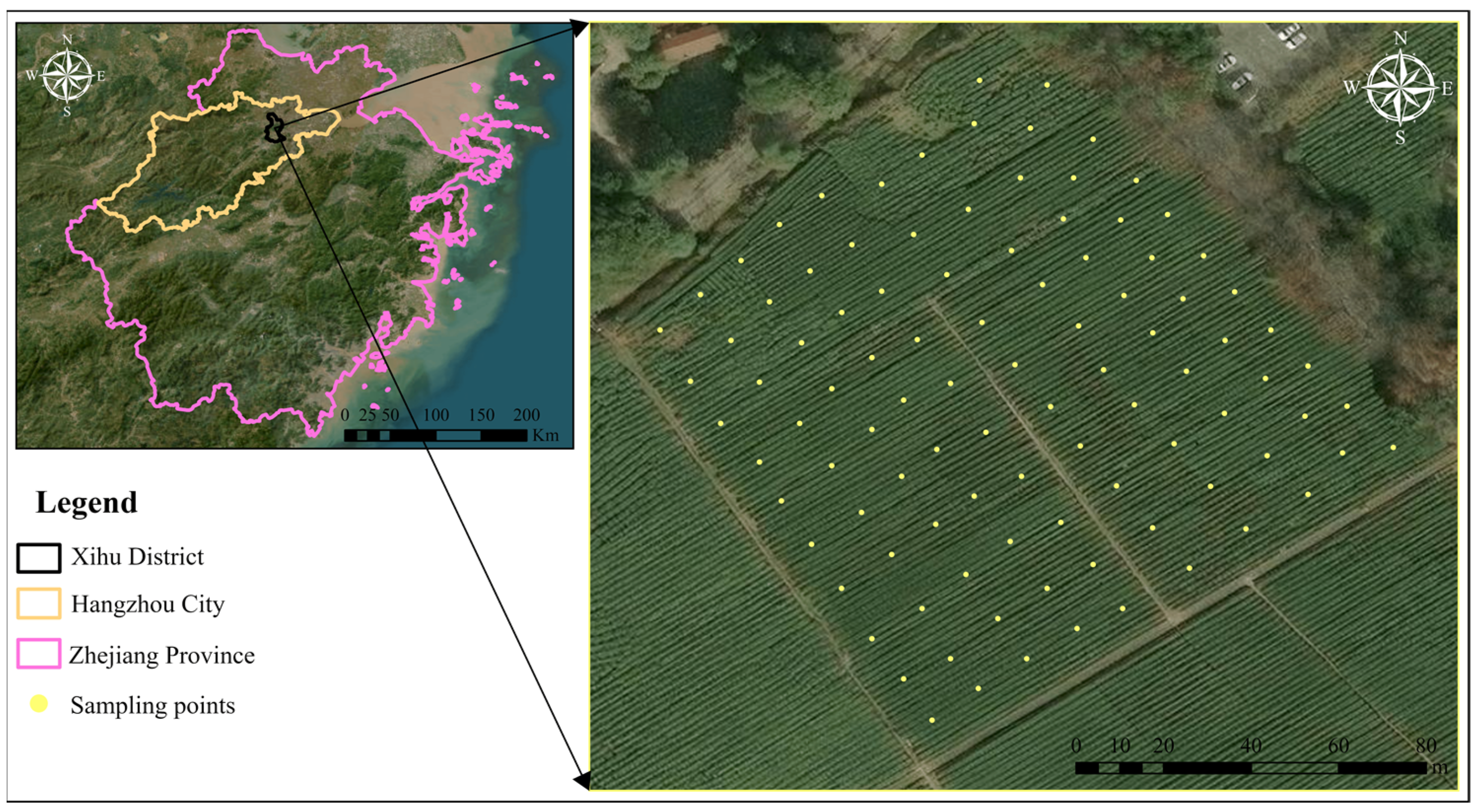
Figure 1. Distribution of tea field locations and sampling points. (Left): geographic location of Xihu District and the Chahui Tea Garden. (Right): spatial distribution of the tea leaf sampling points.
Agriculture 15 01039 g001
Figure 2. Workflow of hyperspectral estimation for tea leaf chlorophyll content, with Part 1 illustrating the acquisition of leaf hyperspectral reflectance and chlorophyll measurements; Part 2 showing preprocessing of raw hyperspectral data and correlation analysis with chlorophyll content; and Part 3 presenting the construction of six individual machine learning models and seventeen stacking models for estimation.
Agriculture 15 01039 g002
Figure 3. (a) Descriptive statistics of tea LCC (SD: standard deviation, CV: coefficient of variation). (b) Range and average spectral curve of tea leaf hyperspectral curve.
Agriculture 15 01039 g003
Figure 4. (a) The correlation coefficient between tea LCC and hyperspectral reflectance of tea leaves; (bd) the red dots indicate the feature bands selected by the SCARS algorithm from the original hyperspectral reflectance curve, the reflectance curve after 1st order derivative transformation, and the reflectance curve after 2nd order derivative transformation, respectively.
Agriculture 15 01039 g004
Figure 5. Based on the prediction of the 0–2-order optimal stacking model and the measured LCC scatter plot, (a) the prediction results of Stacking4 constructed with the original hyperspectral data set as the input parameters of the model; (b) The prediction results of Stacking2, which was constructed with the input parameters of the hyperspectral data set after the first derivative processing; (c) The prediction results of Stacking8, which was constructed with the hyperspectral data set after second-order derivative processing as the input parameters of the model.
Agriculture 15 01039 g005
Figure 6. (ac) Prediction accuracy indices of stacking models constructed with LS-SVM, RF, XGBoost, and BP-AdaBoost as base model combinations and PLSR, RR, SVM, GPR, GRU, and CNN as meta-models, where (a) represents R2, (b) represents RMSE, and (c) represents RPD.
Agriculture 15 01039 g006
Table 1. Pearson correlation analysis results based on 0–2 order hyperspectral data and tea LCC.
OrderPearson Correlation Analysis
PbNbTbR_maxCorresponding Bands/nm
0551502050.615701
11445266700.891736
2109952040.877746
The abbreviations Pb, Nb, and Tb, respectively, correspond to the count of statistically significant positive, negative, and total correlation bands surpassing the 0.01 significance threshold. The parameter R_max indicates the peak absolute correlation coefficient magnitude observed in the analysis.
Table 2. Evaluation results of prediction accuracy index of single model based on 0–2 order.
ModelOrderTraining SetTesting Set
R2RMSEMAEMAPER2RMSEMAEMAPERPD
LS-SVM00.9842.3481.6413.8800.65411.3096.52515.7981.759
11.0000.0140.0100.0240.8018.5826.45316.1522.356
21.0000.0010.0010.0020.7759.1256.96215.3482.119
RF00.7738.7666.22814.0980.56412.69410.18420.8531.526
10.9135.4143.7398.4960.9065.8964.83410.7863.269
20.9274.9663.4248.1520.8876.4575.44211.5932.981
XGBoost00.9872.1071.3453.1160.72410.0897.40415.5521.916
10.9941.3950.6621.7600.8916.3514.99211.9663.027
20.9941.3780.4691.2510.8676.9995.28012.2992.746
LSTM00.8596.9205.01711.8240.9035.9714.67010.6593.224
10.9553.9183.0957.4610.9265.2354.3709.7494.535
20.9931.5001.1322.8850.9095.7824.7209.6233.332
BPNN00.8566.9934.91010.2120.8617.1785.46111.5652.987
10.9245.0792.8676.0030.9085.8404.82311.3303.327
20.8666.7382.9606.6930.8158.2606.75015.0292.404
BP-AdaBoost00.9394.5373.2177.3540.8816.6234.37310.8992.940
10.9613.6392.3835.6680.9185.5034.31510.4783.817
20.9583.7552.9376.4600.8327.8846.40114.1312.475
The units of MAE, RMSE, and RPD are all µg/cm2, and the units of MAPE are %.
Table 3. Twelve kinds of stacking models based on PLSR as a meta-model.
Base Model Assembly Base Model Assembly
Stacking1LS-SVM/BP-AdaBoost/LSTMStacking7RF/BP-AdaBoost/XGBoost
Stacking2LS-SVM/BP-AdaBoost/RFStacking8LS-SVM/RF/LSTM/BP-AdaBoost
Stacking3LS-SVM/BP-AdaBoost/XGBoostStacking9LS-SVM/XGBoost/LSTM/BP-AdaBoost
Stacking4LSTM/BP-AdaBoost/XGBoostStacking10RF/XGBoost/LSTM/BP-AdaBoost
Stacking5LSTM/BP-AdaBoost/RFStacking11LS-SVM/RF/XGBoost/BP-AdaBoost
Stacking6LS-SVM/RF/XGBoostStacking12LS-SVM/RF/XGBoost/LSTM/BP-AdaBoost
Table 4. Evaluation results of prediction accuracy index based on 0–2 order stack model.
ModelOrderTraining SetTesting Set
R2RMSEMAEMAPER2RMSEMAEMAPERPD
Stacking100.8636.8065.26813.1360.9215.4183.8059.7023.811
10.8666.7355.38012.8030.9424.6113.7058.6404.961
20.9195.2324.0839.3330.9384.7913.8268.8174.017
Stacking200.8636.8035.21412.9300.9325.0173.8199.7384.102
10.8537.0705.61113.4610.9514.2543.2647.5374.775
20.9155.3564.2329.6550.9364.8673.9999.3073.949
Stacking300.8696.6695.19912.8110.9334.9593.8829.6714.065
10.8547.0385.66013.7030.9484.3633.2847.7354.672
20.9155.3634.2869.7910.9344.9404.0129.3833.890
Stacking400.8477.2105.83414.1010.9424.6123.6668.8874.350
10.8497.1575.65613.7490.9474.4263.3247.9174.610
20.9155.3744.2009.4120.9344.9434.1609.5763.891
Stacking500.8497.1545.58413.5290.9225.3714.29910.1853.653
10.8656.7625.28712.6260.9464.4493.3867.9005.005
20.9175.2994.1949.4500.9334.9704.0589.1753.877
Stacking600.7499.2156.77216.7510.8178.2285.94413.6212.338
10.7858.5416.56814.9570.9125.6864.80810.4763.384
20.7898.4466.19514.5680.8926.3085.07410.8583.068
Stacking700.8437.3005.59613.6010.9255.2574.1119.9543.800
10.8626.8315.32112.6870.9464.4813.4598.1745.013
20.9185.2784.1229.3080.9374.8143.9258.8964.004
Stacking800.8646.7855.30713.1310.9165.5594.08310.0753.697
10.8686.6825.23312.3630.9484.3793.4457.8995.157
20.9185.2604.0579.3250.9394.7383.7738.6584.065
Stacking900.8696.6565.25512.9240.9235.3463.9249.6123.778
10.8706.6305.18112.3290.9474.4183.4777.9695.081
20.9195.2254.0979.3900.9364.8443.8798.9423.972
Stacking1000.8497.1455.47713.3650.8696.9635.92613.3622.777
10.8666.7365.32512.7730.9434.5773.5268.2634.918
20.9205.2154.0329.0300.9374.8073.9488.9134.010
Stacking1100.8716.6185.17212.8350.9315.0633.9689.9383.954
10.8547.0365.59113.4510.9504.2953.2897.5734.721
20.9165.3304.1799.5080.9364.8754.0189.3673.943
Stacking1200.8696.6655.14012.8120.9185.5144.61411.2293.557
10.8706.6445.15912.2160.9484.3933.4617.8405.100
20.9215.1843.9659.0140.9394.7463.8528.8314.056
The units of MAE, RMSE, and RPD are all µg/cm2, and the units of MAPE are %.
Table 5. Analysis of base model selection differences between three-model and four-model stacking configurations in Stacking1–11.
The Number of Base Models Is 3Add 1 Base ModelThe Number of Base Models Is 4
Stacking1LS-SVM/BP-AdaBoost/LSTMRFStacking8
XGBoostStacking9
Stacking2LS-SVM/BP-AdaBoost/RFLSTMStacking8
XGBoostStacking11
Stacking3LS-SVM/BP-AdaBoost/XGBoostLSTMStacking9
RFStacking11
Stacking4LSTM/BP-AdaBoost/XGBoostLS-SVMStacking9
RFStacking10
Stacking5LSTM/BP-AdaBoost/RFLS-SVMStacking8
XGBoostStacking10
Stacking6RF/LS-SVM/XGBoostLSTMStacking9
BP-AdaBoostStacking11
Stacking7RF/BP-AdaBoost/XGBoostLSTMStacking10
LS-SVMStacking11
Disclaimer/Publisher’s Note: The statements, opinions and data contained in all publications are solely those of the individual author(s) and contributor(s) and not of MDPI and/or the editor(s). MDPI and/or the editor(s) disclaim responsibility for any injury to people or property resulting from any ideas, methods, instructions or products referred to in the content.