CanKiwi: A Mechanistic Competition Model of Kiwifruit Bacterial Canker Disease Dynamics

Abstract

This paper proposes a mathematical model based on a mechanistic approach and previous research findings for the bacterial canker disease development in kiwifruit vines. This disease is a leading cause of severe damage to kiwifruit vines, particularly in humid regions, and contributes to significant economic challenges for growers in many countries. The proposed model contains three parts. The first one is the model of the kiwifruit vine describing its light interception, its carbon acquisition, and the partitioning dynamics. The carbon resource represents the chemical energy required for maintaining the necessary respiration of the living organs and their growth processes. The second part of the model is the dynamics of the pathogenic bacterial population living within the vine’s tissues and competing with them for the carbon resource required for their proliferation. The third part of the model is the carbon dynamics described by a mass conservation formula which computes the remaining amount of carbon available for competition. The model was validated by comparing simulations with experimental results obtained from growth chambers. The results show that the proposed model can simulate reasonably well the functional part of the vine in both the healthy case and the disease case without plant defense mechanisms in which the bacteria are always dominant under favorable environmental conditions. They also show that the environmental effects on the vine’s growth and the infection progress are taken into account and align with the previous studies. The model can be used to simulate the infection process, predict its outcomes, test disease management techniques, and support experimental analyses.

1. Introduction

Kiwifruit Bacterial Canker (KBC) disease, caused by Pseudomonas syringae pv. actinidiae (Psa) bacteria, represents a significant threat to kiwifruit (Actinidia chinensis) production globally resulting in substantial economic losses [1]. Its symptoms include necrotic spots surrounded by yellow halos on the leaves, see Figure 1, blossom necrosis, twig wilting, and bleeding cankers on stems with whitish to red exudate [2]. These symptoms appear only in advanced stages of infection since Psa is a hemibiotrophic bacterium [3]. It behaves as a biotrophic agent during the early infection stages, then as a necrotrophic one, degrading the vine’s tissues after overcoming its defense system, eventually leading to its demise in the late stages of infection [4,5]. Optimal environmental conditions for bacterial proliferation and spread involve high humidity, temperatures ranging between 18 °C and 25 °C, and freezing temperatures during the preceding winter, whereas unfavorable conditions include temperatures exceeding 35 °C and drought [6,7].

Regarding the complexity of the Psa infection process, significant challenges arise when trying to control the disease. Current approaches predominantly rely on chemical bactericides, which provide short-term control but risk diminishing the plant’s natural defenses and fostering bacterial resistance in the long term [8]. Moreover, in advanced infection stages, drastic measures like vine removal become necessary, underscoring the need for more sustainable and integrated disease management strategies [2,9]. The latter require a deep understanding of the infection mechanisms.

Mathematical models have always been a critical tool for studying biological processes and the mechanisms governing them [10,11]. They serve as a virtual twin of the process that can simulate its behaviors, provide quantitative analyses of its components, and test different management procedures to predict their outcomes [12,13]. In this study, we focus on plant growth processes, and the effects of their interaction with both biotic and abiotic environmental factors. Particularly, we focus our study on the interplay between the kiwifruit vine, the Psa bacteria, which is mainly responsible for KBC disease, and their environment, and the resulting impact on the vine’s growth and yield. Models for these kinds of effects still need to be investigated [12]. To our knowledge, there are no previous mathematical models of the physiological interactions between KBC disease and kiwifuit vine in the literature. Existing models, such as the climate suitability model [14] and the infection risk model [15], only focus on estimating the geographical distribution of the disease or its total damage [2,16]. The detailed study of the pathogen effects and their integration into the plant’s model poses a significant challenge due to their diverse and complex nature. Our study addresses this gap by focusing on modeling the impact of Psa on kiwifruit vines, particularly how the Psa competes with the vine for carbon resources. The proposed model can facilitate KBC disease studies, simulate the infection development and increase knowledge in the field of plant–pathogen interactions. It can also be used to explore and test new disease control strategies and predict their outcomes.

Contemporary literature hosts various types of plant models, each tailored to represent a specific process within a particular application case and representation scale. Noteworthy categories include functional models, used to simulate biological phenomena related to plants functioning [17], structural models, used to replicate the geometrical shape of plants [18], and the most recent Functional–Structural Plant Models (FSPMs), which not only consider the relation between plant structure and its biological functioning, but also account for the effects of abiotic environmental factors [19]. Models accounting for the effects of biotic environmental factors are relatively scarce. Constructing such models proves challenging since they integrate the intricate interplay between genetically distinct organisms, or even from different species, including various types of symbiotic relationships [20,21]. Despite this challenge, these models are of substantial importance in predictive ecology, population dynamics, community dynamics, and crop management [20,22].

FSPMs have recently found application in modeling fruit crops, and additional challenges arise in this case of perennials [23]. Among the existing models, we can find, for instance, the L-PEACH model for peaches (Prunus persica) [24], the L-ALMOND model for almonds (Prunus dulcis) [25], the GrapevineXL model for the common grapevine (Vitis vinifera) [26,27], the V-Mango model for mangoes (Mangifera indica) [28], the MappleT model for apples (Malus domestica) [29,30], and the L-KIWI model for the kiwifruit vine (Actinidia chinensis var. deliciosa) [31], among others. These models use a Lindenmayer systems (L-systems) framework to replicate the plant’s 3D structure in simulation, and differential equations or Markov chains for the functional part concerning photosynthesis, carbon dynamics, nutrient transportation, and the growth of organs [32].

The integration of biotic effects into existing FSPMs poses a significant challenge due to the diverse origins and manifestations of these effects. For instance, we have the positive effect of the mycorrhizal fungi, which has been analyzed in [22,33] and combined with a plant model in [21]. We can also find mathematical models for negative effects, for example, in some plant–insect interactions [34], herbivore effects [35,36], and pathogen and pest effects with a focus of interest on the plant’s structure [37,38,39].

In our work, we focus on modeling the effects of pathogens on the plant’s functioning, particularly the PSA bacteria which is responsible for KBC disease. While various disease models exist, our interest lies in understanding the dynamics of the KBC. Previous studies [40,41,42,43] provide detailed insights and reviews on modeling approaches for similar diseases. Notable models include the mummy berry disease model [44] serving as a decision support system for disease management in the USA, a mechanistic weather-driven model [45] for Ascochyta rabiei infection in chickpeas, a ripe rot disease model [13] including the effects of the environment and the host plant on the development of Colletotrichum fungi responsible for the ripe rot of grapes, a mechanistic model for downy mildew infection in grapevines used for infection prediction [46], and a general model exploring the effects of crop management procedures on plant disease epidemics [47].

Existing mathematical models of KBC include the climate suitability model [14], which is analogous to geographical distribution models [48,49] and the infection risk model [15]. In these models, the potential geographical distribution of the disease is computed using different methods. These models use forecasts of weather data, either empirically or semi-mechanistically, to predict areas at high risk of future Psa infection. Additionally, there are the accumulated potential damage model [2] and the productivity impact model [16]. In [2], a mathematical model for estimating the accumulated potential damage caused by PSA on kiwifruit canes during the growing and wintering seasons by computing the amount of symptoms was proposed. However, this model does not account for temperature effects on disease development, nor does it consider vine growth, being developed under the assumption of fixed-size vines with a cane diameter of approximately 10 mm. Finally, in [16], a statistical approach was used to analyze productivity data in 2599 orchards and quantify the impacts of PSA infection and its management practices on productivity.

Therefore, the present study had two specific objectives. The first one consisted of modeling the Actinidia–Psa interaction during the infection and bacterial colonization process, focusing on the in planta competition for carbon (Section 2) through integrating several components with biochemical, physiological, and population dynamics significance. The second one consisted of simulating the obtained model under realistic environmental conditions and comparing its outcomes with experimental results to assess the model’s performance (Section 3). Moreover, as a general objective, this work aimed at providing a basic model on KBC progression in kiwifruit vines that could assist in the development of Psa control methods and possibly in the transferring of knowledge to study other pathosystems.

2. Material and Methods

In this section, we introduce a mechanistic competition model for kiwifruit bacterial canker disease dynamics, abbreviated as the CanKiwi model. The proposed model is illustrated in Figure 2. Unlike conventional approaches, we embed the disease model as a sub-component within the vine’s FSPM. Within this sub-model, we use population dynamics principles [50,51,52,53] to simulate the proliferation of PSA bacteria in the vine [54]. Additionally, we explicitly account for the local environmental conditions and the host effects [51]. However, to avoid high computational complexity, we focus solely on the temporal dynamics of the infection related to the functional part of the competition on carbon resource between PSA bacteria and the Kiwifruit vine formulated as a state-space model [55]. The structural part of the infection dynamics is discarded to avoid high complexity. The rationale behind this will be elaborated later in this paper. The kiwifruit model proposed by [31] is considered as a basis for this infection modeling study. The structural part of the model is kept as is, while its functional part is improved as per the following sections and used in KBC disease modeling.

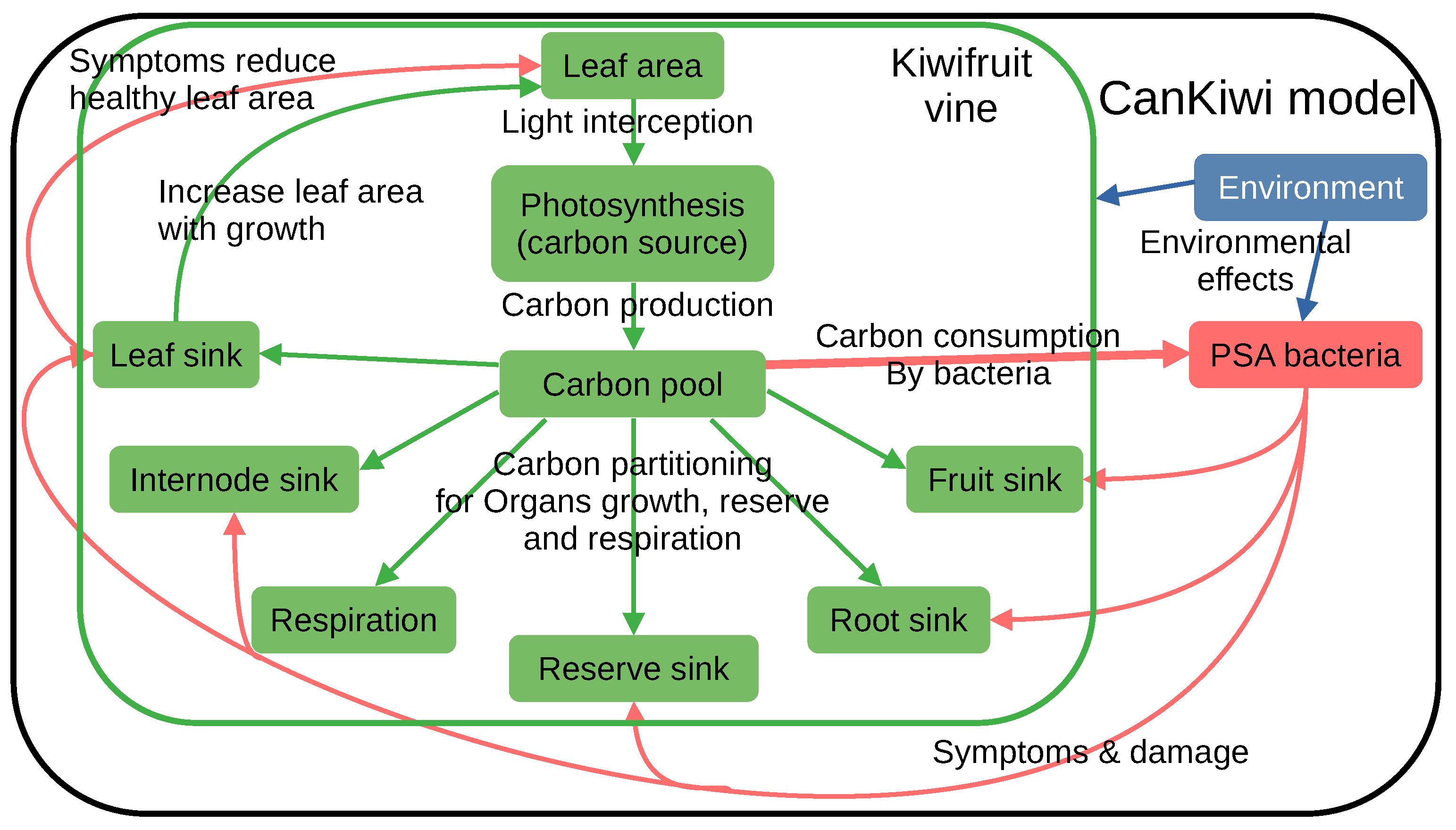
2.1. The Functional Kiwifruit Model

The functional part of the model is a state space representation of carbon dynamics within the plant expressed in terms of dry matter. Carbon is acquired through photosynthesis, and it then flows from its sources (leaves) via the transportation tissues (phloem) until it reaches the sinks (growing organs and storage organs). Therefore, we are developing a source-to-sink model capturing the flow of carbon taken up by leaves into different types of organs depending on their sink capacity. For each organ, this model considers the growth, maintenance of respiration, storage as starch in plant reserves, and carbon acquisition, which vary depending on the type of organ.

2.1.1. Carbon Acquisition (Photosynthesis)

Plant carbon acquisition through photosynthesis is typically estimated from a simulation of light distribution over the vine [56]. To reduce computational complexity, we have opted to use an equation proposed by [17], which reads as follows:

$$I_{0,t}={\overline{I}}_0{\displaystyle \frac{\pi }{2}}sin\left({\displaystyle \frac{\pi t}{p}}\right),0\le t\le p$$

(1)

where $I_{0,t}$ is the irradiance, ${\overline{I}}_0$ its daily average, and p is the photoperiod. Notice that this amount of irradiance should be converted to photosynthetic photon flux density (PPFD) $I_t$ absorbed by the leaves in the 400 to 700 nm waveband. The conversion factor from irradiance $I_{0,t}$ to PPFD $I_t$ is not fixed and depends on the geographical location and its local weather conditions [57]. In our simulation, we use the approximated value of 1 ${\text{w/m}}^2\approx$ 4.57 mol PAR ${\mathrm{m}}^{-2}$${\mathrm{s}}^{-1}$ corresponding to sunlight irradiance [58].

Additionally, according to [17], the daily temperature distribution is given by the following equation:

$$T_t={\tau }_1+{\tau }_{2}sin\left({\displaystyle \frac{\pi }{p}}\left(t-\varphi \right)\right),0\le t\le p$$

(2)

where

$${\tau }_1={\displaystyle \frac{\overline{T}-\left(2T_m/\pi \right)cos\left(\pi \varphi /p\right)}{1-\left(2/\pi \right)cos\left(\pi \varphi /p\right)}}$$

$${\tau }_2={\displaystyle \frac{T_m-\overline{T}}{1-\left(2/\pi \right)cos\left(\pi \varphi /p\right)}}$$

In the above, $T_m$ is the maximum daily temperature at afternoon $t=p/2+\varphi$, $\overline{T}$ is its daily average, and $\varphi$ = 10,800 s = 3 h is the time-shift of the maximum temperature from mid-day. An example of the curves representing the daily irradiance and temperature distributions is given in Figure 3.

The Gross photosynthesis $P_{gross,t}$ of each leaf is then estimated using the following function [59]:

$$P_{gross,t}=P_{max}tanh\left(I_t{\phi }_{app}/P_{max}\right)$$

(3)

where $P_{max}$ is the maximum photosynthesis rate, ${\phi }_{app}$ is the apparent photon yield, and I is the photosynthetic photon flux density absorbed by the leaf. The estimated maximum PPFD at the top of the canopy in a midsummer clear sky is $I_{max}$ = 1300 $\mathsf{\mu }$mol PAR ${\mathrm{m}}^{-2}$${\mathrm{s}}^{-1}$.

2.1.2. Carbon Inflow into Sinks for Organ Growth

Organ growth rate can be determined by its intrinsic potential growth and the amount of carbon flow into the sink. Carbon is distributed over the growing organs based on their respective priorities, which may vary with the seasons. Let f be the function describing the growth rate due to carbon flow into the organ’s sink depending on its priority, and G the function describing the organ’s intrinsic growth rate depending on its type and the environmental condition regulated by the vine’s genome. Consequently, the growth in an organ’s sink size is supposed to follow the equation proposed in [31] and can be written as

$${\displaystyle \frac{d{s}_{i,t}}{dt}}=f\left(q_i,c_t\right)G_{max}\left(·\right)$$

(4)

where $s_{i,t}$ is the size of the sink of type i, $c_t$ is the amount of carbon available, $q_i$ is a parameter controlling sink priority, and $G_{max}\left(·\right)$ is the maximum intrinsic potential growth of the organ depending on environmental condition and sink’s type. In (4), the function $f\left(q_i,c_t\right)$ is the same for all the sinks and is given by

$$f\left(q_i,c_t\right)={\displaystyle \frac{c_t}{q_i+c_t}}$$

(5)

where it can be noticed that, by increasing the value of $q_i$, the carbon inflow into the sink size $s_{i,t}$ will decrease and its growth will then be limited.

2.1.3. Vegetative Growth

Vegetative growth is represented by two state variables $s_{i,t}$ and ${\alpha }_{i,t}$, where the former signifies the size of sink i, and the latter indicates its developmental age. In the context of vegetative growth, the type i can represent either a leaf, an internode, or a root. The developmental age variable ${\alpha }_{i,t}$ serves to constrain the organ’s growth to its final potential size. It accounts for the effects of different environmental conditions on growth, thus replacing the conventional thermal time concept found in other plant models. This approach enables the consideration of a non-linear response, which is unattainable with thermal time. The developmental age is presumed to be proportional to the organ’s maximum specific growth rate, implying that it is inversely proportional to the duration of rapid growth ${\tau }_i\left(T_t\right)$, as shown by the following equation proposed by [60]:

$${\displaystyle \frac{d{\alpha }_{i,t}}{dt}}={\displaystyle \frac{1}{{\tau }_i\left(T_t\right)}}$$

(6)

where $T_t$ is the temperature. More details about this concept are given in [31].

The developmental age variable is used as an input in a growth function, representing the relative growth rate of an organ, given by

$${\displaystyle \frac{d{s}_{i,t}}{dt}}={\displaystyle \frac{1}{{\tau }_i\left(T_t\right)}}{s}_{i,t}\Gamma \left({\alpha }_{i,t}\right)$$

(7)

where ${\displaystyle \frac{1}{{\tau }_i\left(T_t\right)}}$ is the maximum specific growth rate, and $\Gamma \left({\alpha }_{i,t}\right)$ is a logistic growth function given by

$$\Gamma \left({\alpha }_{i,t}\right)={\displaystyle \frac{1}{1+exp\left({\alpha }_{i,t}-{\beta }_i\right)}}$$

(8)

where ${\beta }_i$ is a scaling parameter used to avoid using negative values of developmental age.

The leaf growth rate can then be computed in the same way proposed by [60] as follows:

$${\displaystyle \frac{d{s}_{leaf,t}}{dt}}=f\left(q_{leaf},c_t\right)\left({\displaystyle \frac{\Gamma \left({\alpha }_{leaf,t}\right)\left(s_{leaf,t}-B\left(n\right)\right)}{{\tau }_{leaf}\left(T_t\right)}}\right)$$

(9)

where $B\left(n\right)$ represents the initial growth rate depending on the node number n. $f\left(q_{leaf},c_t\right)$ and $\Gamma \left({\alpha }_{leaf,t}\right)$ are as defined before in Equations (5) and (8), respectively, and $G_{max}\left(·\right)$ is the second term on the r.h.s. (right-hand side) of Equation (9). Then, leaf area $A_{leaf,t}$ can be approximated from leaf sink size by $A_{leaf,t}=L{s}_{leaf,t}$, where the constant L (${\mathrm{m}}^2$${\mathrm{g}}^{-1}$C) is the specific leaf area of the vine.

The internode growth rate is characterized by an expansion in volume to enhance its carbon transportation capacity and an increase in its sink size. These two variables are proportional to each other and can be described by the equation $s_{inde,t}=\rho V_t$, where $\rho$ is the volumetric density, and $V_t$ is the volume of the internode, which can be split into radial and axial growth [61]. We can now use the relative growth rate to formulate the equations of the internode’s growth in length $l_t$ and radius $r_t$:

$${\displaystyle \frac{d{l}_t}{dt}}=f\left(q_{inde,pri},c_t\right)\left({\displaystyle \frac{\Gamma \left({\alpha }_{inde,t}\right)l_t}{{\tau }_{inde}\left(T_t\right)}}\right)$$

(10)

$${\displaystyle \frac{d{r}_t}{dt}}=f\left(q_{inde,sec},c_t\right)\left({\displaystyle \frac{k_{sec}+k_{logistic}\Gamma \left({\alpha }_{inde,t}\right)r_t}{{\tau }_{inde}\left(T_t\right)}}\right)$$

(11)

where $q_{inde,pri}$ and $q_{inde,sec}$ are parameters to control sink priority for primary and secondary growth, respectively, while $k_{sec}$ and $k_{logistic}$ are parameters to control the long-term and the initial rapid radial growth, respectively, to describe the thickening of the internode.

Now, the two previous equations can be combined to obtain the internode’s growth rate, as follows:

$${\displaystyle \frac{d{s}_{inde,t}}{dt}}=\rho {\displaystyle \frac{d{V}_t}{dt}}=\pi r_t^2\rho {\displaystyle \frac{d{l}_t}{dt}}+2\pi r_t{l}_t\rho {\displaystyle \frac{d{r}_t}{dt}}$$

(12)

This equation can be expressed as follows:

$$\begin{array}{c}{\displaystyle \frac{d{s}_{inde,t}}{dt}}=f\left(q_{inde,pri},c_t\right)\left({\displaystyle \frac{\Gamma \left({\alpha }_{inde,t}\right)s_{inde,t}}{{\tau }_{inde}\left(T_t\right)}}\right)\hfill \\ \hfill \hspace{1em}\hspace{1em}\hspace{1em}\hspace{1em}\hspace{1em}\hspace{1em}\hspace{1em}\hspace{1em}\hspace{1em}+f\left(q_{inde,sec},c_t\right)\left({\displaystyle \frac{k_{sec}{A}_{inde,t}\rho +k_{logistic}\Gamma \left({\alpha }_{inde,t}\right)s_{inde,t}}{{\tau }_{inde}\left(T_t\right)}}\right)\end{array}$$

(13)

where $A_{inde,t}=2\pi r_t{l}_t$ is the surface area of the internode.

The relative growth rate of roots is strongly influenced by temperature changes, reaching its maximum potential growth rate in late summer. When including this relative growth rate into the equation of roots sink size, we obtain the following formula derived from the method proposed by [62]:

$${\displaystyle \frac{d{s}_{root,t}}{dt}}=f\left(q_{root},c_t\right)k_{prgr}{s}_{root,t}{e}^{T_{prgr}\left(T_t-20\right)}$$

(14)

where $k_{prgr}$ is a parameter controlling the maximum potential growth rate in the peak time, and $T_{prgr}$ is a parameter to control the response of growth rate to temperature.

2.1.4. Fruit Growth

Kiwifruit grows in two phases, both of which follow a sigmoid growth rate curve where the first phase is faster than the second [63]. The change in fruit sink size in this case can be computed by the following equation:

$${\displaystyle \frac{d{s}_{fruit,t}}{dt}}=f\left(q_{fruit},c_t\right)k_1\left({\displaystyle \frac{0.5}{1+exp\left({\alpha }_{fruit,t}-k_2\right)}}+{\displaystyle \frac{0.5}{1+exp\left({\alpha }_{fruit,t}-k_3\right)}}\right)s_{fruit,t}$$

(15)

where ${\alpha }_{fruit,t}$ is the developmental age of the fruit, and $k_1$, $k_2$, and $k_3$ are parameters controlling the fruit growth rate in the two-phase growth. The temperature effect on the potential fruit growth rate and final fruit size still needs to be investigated.

2.1.5. Maintenance of Respiration

The carbon required to maintain the respiration of an organ $M_{rsp,i,t}$ depends on its total biomass and temperature. A maintenance sink is used to describe the carbon required for the respiration of an organ i, as shown by the following equation proposed by [62]:

$$M_{rsp,i,t}=f\left(q_{rsp,i},c_t\right)s_{i,t}{m}_i{e}^{T_{rsp,i}\left(T_t-20\right)}$$

(16)

where $q_{rsp,i}$ is the respiration sink priority for organ type i, $s_{i,t}$ is its sink size, and $m_i$ and $T_{rsp,i}$ are its coefficients of maintenance and temperature response of the respiration, respectively.

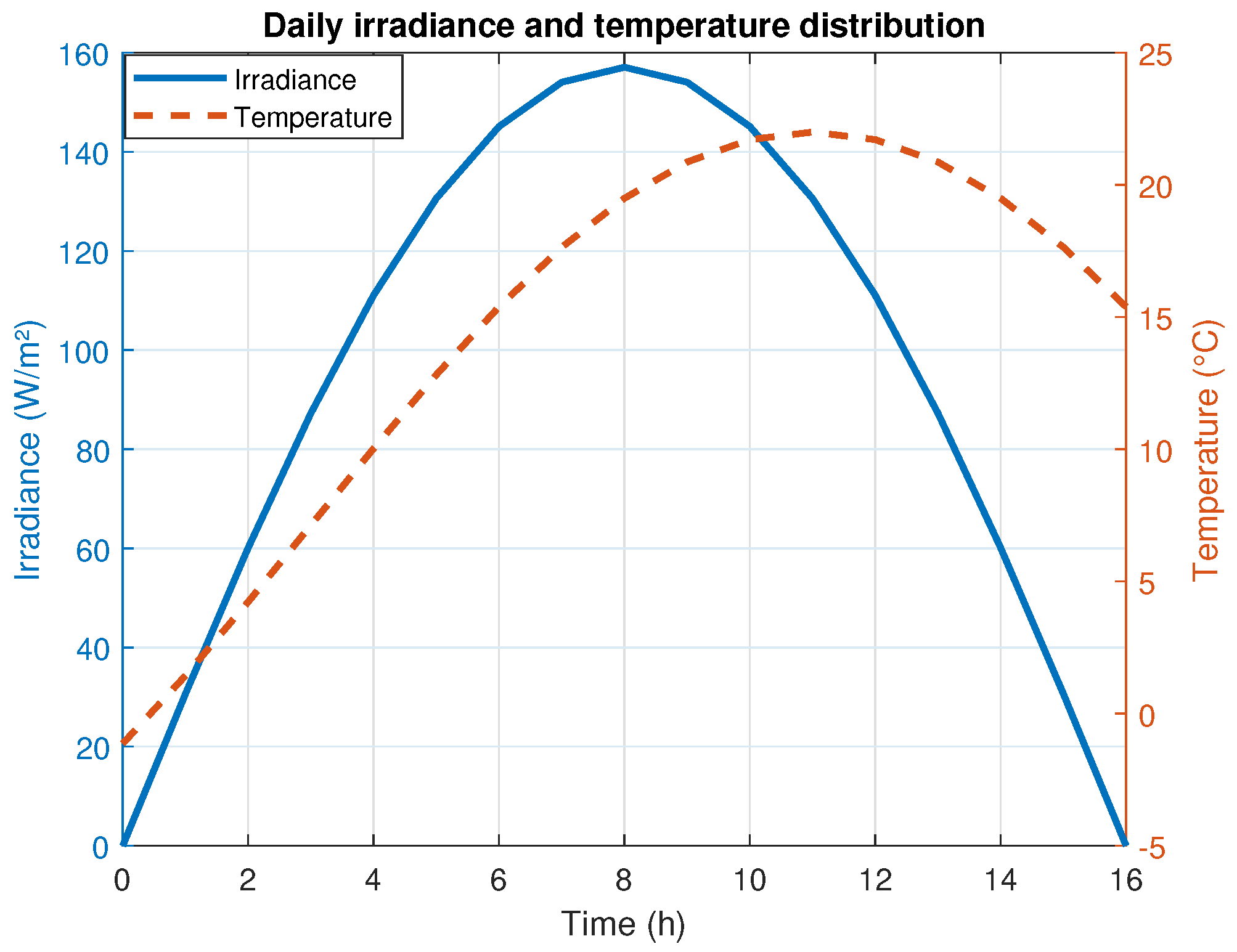
2.1.6. Carbon Acquisition Dynamics

The amount of carbon acquired by the leaves is modeled as a photosynthetic carbon pool of size $s_{src}$. This carbon is then moved to the phloem for transportation and distribution to the different organs according to their priority, which depends on the carbon amount in each one of them and in the transporting phloem [64]. The change in size of the photosynthetic carbon pool is assumed to be given by

$${\displaystyle \frac{d{s}_{src,t}}{dt}}=g\left(q_{src},c_t\right)P_{gross,t}\sigma L\left(1-{\displaystyle \frac{s_{src,t}}{s_{leaf,t}}}\right)s_{src,t}$$

(17)

where we can see that the carbon acquired through photosynthesis is limited by the leaf’s capacity, represented by the its current sink size $s_{leaf,t}$. $\sigma$ is a constant unit conversion coefficient (from $\mathsf{\mu }$mol ${\mathrm{CO}}_2$ to gC), and $g\left(q_{src},c_t\right)$ is a limiting function for carbon flow given by

$$g\left(q_{src},c_t\right)=1-{\displaystyle \frac{c_t}{q_{src}+c_t}}$$

(18)

where $q_{src}$ is a parameter regulating the carbon supply rate.

2.1.7. Reserve Dynamics

Carbon is stored in the form of starch at the internodes and roots levels. Each one of these organs can store an amount of synthesized starch proportional to its size up to a certain capacity. When needed, stored carbon can be re-mobilized and used, and the quantity of re-mobilized carbon depends on the carbon amount outside the reserve and the existing amount within it [64]. Therefore, we can use the following equation to depict the change in the storage sink size:

$${\displaystyle \frac{d{s}_{res,i,t}}{dt}}=f\left(q_{syn},c_t\right)\left(1-{\displaystyle \frac{s_{res,i,t}}{s_{i,t}{s}_{max,i}}}\right)k_{starch}{k}_{syn}{s}_{res,i,t}-g\left(q_{hyd},c_t\right){\displaystyle \frac{k_{hyd}}{k_{starch}}}{s}_{res,i,t}$$

(19)

where the first part in the r.h.s. of the equation is for carbon storage (starch synthesis), happening at rate $k_{syn}$ depending on the carbon amount $c_t$ outside the reserve. Carbon storage is limited at the maximum capacity $s_{max,i}$ depending on the size $s_{i,t}$ of organ i. $k_{starch}$ refers to the amount of starch that can be synthesized from 1 g of carbon. The second term in the r.h.s. of the equation is for carbon re-mobilization (starch hydrolysis), happening at rate $k_{hyd}$, depending on the stored amount of starch and on the carbon amount outside the reserve.

2.2. Bacterial Population Dynamics

This section focuses on modeling the dynamics of PSA bacteria population. We start by considering that the bacterial population size increases exponentially in optimal environmental, physiological, and nutritional conditions as given by the Malthusian model $d{x}_t/dt=\mu x_t$, where $x_t$ is the size, density, or concentration of the population, and $\mu$ is the growth rate defined by the difference between birth rate b and death rate d. Sub-optimal environmental, physiological, and nutritional conditions interfere in this growth model to penalize the growth and reduce its infinite exponential increase. To represent this interference, we propose the following modified model:

$$\begin{array}{c}{\displaystyle \frac{d{x}_t}{dt}}={\displaystyle \frac{q_t}{1+q_t}}{\mu }_{max}{\displaystyle \frac{S_t}{k_s+S_t}}{h}_{t}exp\left(-{\displaystyle \frac{{\left(T_t-T_{opt}\right)}^2}{T_{range}}}\right)\left(1-{\displaystyle \frac{x_t}{x_{max}}}\right)x_t\hfill \\ \hfill \hspace{1em}\hspace{1em}\hspace{1em}\hspace{1em}\hspace{1em}\hspace{1em}\hspace{1em}\hspace{1em}\hspace{1em}\hspace{1em}\hspace{1em}\hspace{1em}\hspace{1em}\hspace{1em}\hspace{1em}\hspace{1em}\hspace{1em}-\left(1-h_t\right){\displaystyle \frac{0.05}{0.05+exp\left(T_{max}-T_t\right)}}{x}_t\end{array}$$

(20)

where the first part of the r.h.s. of this equation represents the increase in population size due to bacteria cells division, while the second part represents the decrease in population size due to cell death. The term ${\displaystyle \frac{q_t}{1+q_t}}$ is known as the adjustment function [65], which depends on the physiological state of the bacteria $q_t$. This function describes the bacteria’s ability to reproduce upon entering a new environment (the vine), and its impact on population size. The adjustment function introduces a delay in the exponential growth curve representing the time taken by the bacteria to adapt to their new environment. The physiological state $q_t$ of the bacteria is a state variable, and its dynamics are assumed to be given by [65]

$${\displaystyle \frac{d{q}_t}{dt}}=\nu q_t$$

(21)

where $\nu$ is the rate of adaptation of the bacteria to the new environment. The delay taken by the bacteria to adapt to their environment decreases when their initial physiological state $q_{t_0}$ representing their maturity or ability to reproduce at the time of inoculation $t_0$ increases, and $q_{t_0}$ depends on the past treatment of the bacteria.

The term $\mu ={\mu }_{max}{\displaystyle \frac{S_t}{k_s+S_t}}$ is a Monod-type growth function used to relate the growth rate to the amount or concentration of a specific nutrient $S_t$. The parameters ${\mu }_{max}$ and $k_s$ are the maximum growth rate and the half saturation constant, respectively. The nutrient in this case is the carbon available to the bacteria, thus it is supposed that $S_t=c_t$, which is the same carbon amount available for the vine’s sinks.

The parameter $h_t$ represents the relative humidity, whereas $\left(1-h_t\right)$ in the second part of the equation represents humidity deficit. It is recognized that the bacterial infection propagates rapidly in a humid environment and the severity of the infection increases proportionally to humidity, while it completely disappears in a dry environment.

The positive temperature effect on the growth rate is modeled by a bell-shaped curve given by $exp\left(-{\displaystyle \frac{{\left(T_t-T_{opt}\right)}^2}{T_{range}}}\right)$, where the growth rate reaches its peak value of $100\%$ of the maximum potential growth rate at an optimal temperature value $T_{opt}$ and decreases gradually when the temperature value moves away from $T_{opt}$ until reaching 0. The parameter $T_{range}$ modifies the temperature range tolerated by the bacteria.

On the other side, the negative temperature effect on the growth rate is modeled by a sigmoid function ${\displaystyle \frac{0.05}{0.05+exp\left(T_{max}-T_t\right)}}$ that starts at a temperature value $T_{max}$ representing the maximum temperature tolerated by the bacteria population at which it starts to decrease, and is saturated at a maximum death rate of 1. The function can be modified by changing the preset values $0.05$.

The term $\left(1-{\displaystyle \frac{x_t}{x_{max}}}\right)$ represents a limitation of the bacteria population size depending on their environment capacity, referring to how much bacteria a kiwi vine can accommodate. The bacteria population in the studied vine or orchard can grow up to a maximum value $x_{max}$ depending on the vine’s total biomass. At this maximum value, the studied vine or orchard is supposed to be saturated, meaning that it is at the final stage of infection.

For simplification reasons, we suppose that the studied vine or orchard is a closed bacterial environment. The spacial dynamics of the infection in this case, including the amounts of bacteria entering or exiting the vine, are not taken into account, since they entail the implementation of a reaction diffusion model and the resolution of complicated high dimensional partial differential equations in addition to Equations (20) and (21). This also explains why the infection effects on the structural part of the kiwifruit model are not considered in this first version of the CanKiwi model. Incorporating the spacial dynamics of the vine alongside those of the bacteria will further complicate the model and can even make it intractable. In our case, the disease simulation using the model (20) and (21) starts at the instant of bacterial infection or inoculation into the studied vine. The amount of inoculated bacteria and their physiological state at that time serve as initial values $x_0$ and $q_0$ in our model, respectively.

2.3. Competition for Resources (Carbon Balance)

The dynamics of carbon resource produced in the leaves and consumed by the different vine’s organs and the bacteria can be derived from the following mass balance principle:

$${\displaystyle \frac{d{c}_t}{dt}}={\displaystyle \frac{d{s}_{src,t}}{dt}}-{\displaystyle \frac{d{s}_{leaf,t}}{dt}}-{\displaystyle \frac{d{s}_{inde,t}}{dt}}-{\displaystyle \frac{d{s}_{root,t}}{dt}}-{\displaystyle \frac{d{s}_{fruit,t}}{dt}}-M_{rsp,t}-{\displaystyle \frac{d{s}_{syn,i,t}}{dt}}+{\displaystyle \frac{d{s}_{hyd,i,t}}{dt}}-K_{bct}{\displaystyle \frac{d{x}_{b,t}}{dt}}$$

(22)

where $c_t$ is the carbon amount at time t, and the terms in the r.h.s of the equation represent the rates of carbon production in the leaves, carbon consumption for the growth of leaves, internodes, roots, and fruits, and, for respiration, carbon synthesis as starch, carbon re-mobilization from storage, and carbon consumption by the bacteria at time t, respectively. These rates are computed separately according to their corresponding source of variation. We have ${\displaystyle \frac{d{s}_{syn,i,t}}{dt}}-{\displaystyle \frac{d{s}_{hyd,i,t}}{dt}}={\displaystyle \frac{d{s}_{res,i,t}}{dt}}$; ${\displaystyle \frac{d{x}_{b,t}}{dt}}$ is the first part in the r.h.s. of Equation (20), indicating the reproduction rate, and $K_{bct}$ is the rate of carbon consumption by one colony forming unit (CFU) of bacteria for reproduction.

2.3.1. Biotrophy Stage

Biotrophy is the stage of infection where the bacteria live in the vine and feed on it without causing noticeable symptoms. By consuming the vine’s resources, the bacteria will reduce the vine’s potential growth, especially when weather conditions favor their activity. This reduction in growth is noticed on the obtained simulation results.

2.3.2. Necrotrophy Stage

Necrotrophy is the stage of infection where the bacteria destroy the plant tissues either by releasing substances into them or by clogging the nutrient transportation tissues. In this case, the tissues of the leaves and the internodes start to deteriorate, subsequently affecting other organs like fruits. This results in the appearance of the aforementioned symptoms and a further decline in the vine’s potential growth. The necrotrophy stage is supposed to start when the bacteria population size $x_t$ exceeds a certain threshold $x_{tre}$ [7]. To model tissue necrosis, a negative term $-k_{x,i}{x}_t$ proportional to the bacteria population size is added to the equations of leaf (9), internode (13), and fruit (15) sinks. Here, $k_{x,i}$ is the parameter controlling the rate of tissues death in organ i based on the bacteria population size. Additionally, during the necrotrophy stage, symptoms typically begin to manifest. We propose to represent them in the model by the following equation:

$${\displaystyle \frac{d{S}_{x,i,t}}{dt}}=k_{x,i}{x}_t$$

(23)

where $S_{x,i,t}$ are the symptoms in organ i, and they are exactly the necrotic tissues resulting from the infection. The presence of necrotic tissues in the leaves reduces the photosynthetic area of leaves, which can be seen in photosynthesis simulation results.

3. Results and Discussion

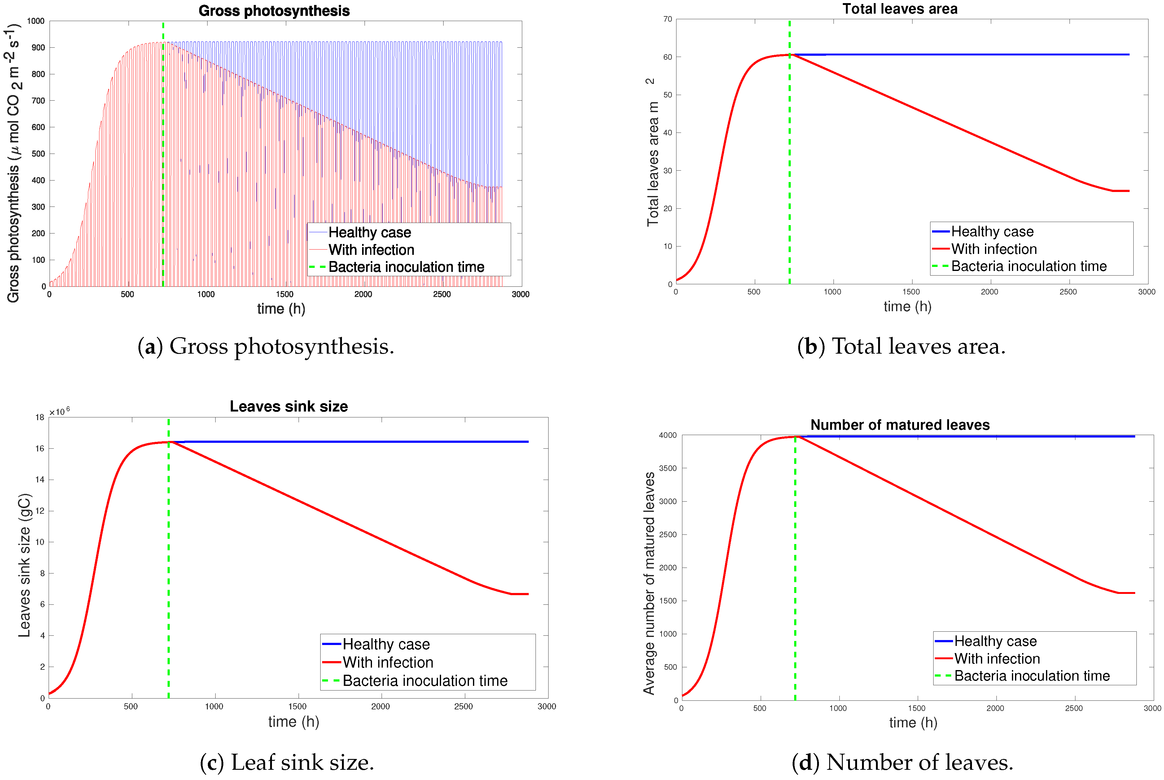
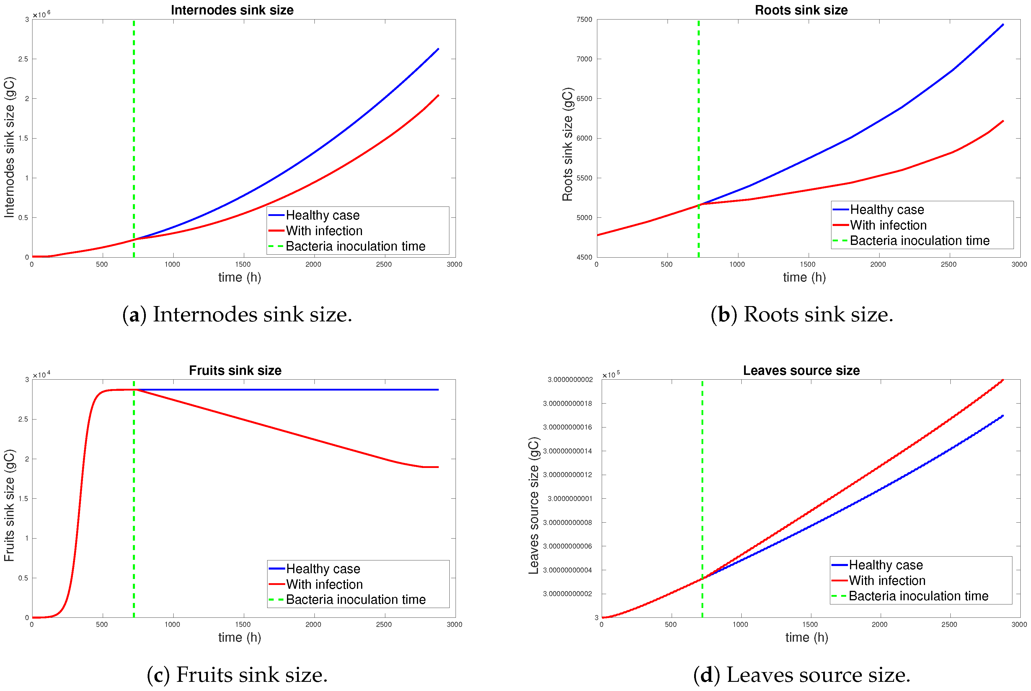
3.1. Simulation Results

The proposed model was implemented in Matlab using the parameter values given in

Table 1. Parameters of the model and their values as used in the simulation.

Parameter	Meaning	Value & Unit
t	Time	1…2880 h
${\overline{I}}_0$	Daily average of irradiance	100 ${\text{w/m}}^2$
$\overline{I}$	Daily average photosynthetic photon flux density absorbed by leaves	457 $\mathsf{\mu }$mol PAR ${\mathrm{m}}^{-2}$${\mathrm{s}}^{-1}$
p	Photoperiod	16 h
$P_{max}$	Maximum rate of photosynthesis	15.2 $\mathsf{\mu }$${\mathrm{molCO}}_2$${\mathrm{m}}^{-2}$${\mathrm{s}}^{-1}$
${\phi }_{app}$	Apparent photon yield	0.039 ${\mathrm{molCO}}_2$${\mathrm{mol}}^{-1}$PAR
${\tau }_{leaf}$	Duration of rapid growth of leaves	68.57 h
${\beta }_i$	Scaling parameter for developmental age	4 dimensionless
$q_{leaf}$	Sink priority for leaf growth	0.01 gC
n	Node number	1 dimensionless
$B\left(n\right)$	Initial growth rate depending on node number n	0 gC
L	Specific leaf area	$3.69\times {10}^{-6}$ ${\mathrm{m}}^2$${\mathrm{g}}^{-1}$C
$\rho$	Internode volumetric density	$1.89\times {10}^{-7}$ ${\mathrm{gCm}}^{-3}$
${\tau }_{inde}$	Duration of rapid growth of internodes	34.285 h
$q_{inde,pri}$	Sink priority for internode elongation	0.01 ${\mathrm{gCm}}^{-3}$
$q_{inde,sec}$	Sink priority for internode thickening	0.05 ${\mathrm{gCm}}^{-3}$
$k_{logistic}$	Rapid initial internode thickening rate	0.28 dimensionless
$k_{sec}$	Long-term internode thickening rate	0.003 dimensionless
$q_{root}$	Sink priority for root growth	30 gC
$k_{prgr}$	Maximum potential growth rate for fibrous root	0.003 ${\mathrm{gCg}}^{-1}$${\mathrm{Ch}}^{-1}$
$T_{prgr}$	Coefficient of root growth response to temperature	$ln\left(2\right)/10$ dimensionless
${\tau }_{fruit}$	Duration of rapid growth of fruits	34.285 h
$q_{fruit}$	Sink priority for fruit growth	30 gC
$k_1$, $k_2$, $k_3$	Parameters controlling fruit growth rate	0.8, 3, 9
$q_{rsp,i}$	Sink priority for maintaining respiration of sink i	$1\times {10}^{-4}$ gC
$m_{leaf}$	Coefficient of maintenance respiration for leaf	$3.3583\times {10}^{-4}$ ${\mathrm{gCg}}^{-1}$${\mathrm{Ch}}^{-1}$
$m_{inde}$	Coefficient of maintenance respiration for internode	$2.1958\times {10}^{-4}$ ${\mathrm{gCg}}^{-1}$${\mathrm{Ch}}^{-1}$
$m_{root}$	Coefficient of maintenance respiration for root	$7.6667\times {10}^{-5}$ ${\mathrm{gCg}}^{-1}$${\mathrm{Ch}}^{-1}$
$m_{fruit}$	Coefficient of maintenance respiration for fruit	0.0596 ${\mathrm{gCg}}^{-1}$${\mathrm{Ch}}^{-1}$
$T_{rsp,i}$	Respiration temperature response coefficient for organ type i	$ln\left(2\right)/10$ dimensionless
$\sigma$	Constant units conversion coefficient	0.0432 gC s $\mathsf{\mu }$${\mathrm{mol}}^{-1}$${\mathrm{CO}}_2$ ${\mathrm{h}}^{-1}$
$q_{src}$	Parameter regulating the leaf carbon supply rate	1 gC
$k_{syn}$	Starch synthesis rate	0.1 ${\mathrm{d}}^{-1}$
$k_{hyd}$	Starch hydrolysis rate	1 ${\mathrm{d}}^{-1}$
$k_{starch}$	Amount of starch made from 1 g of C	2.5 g starch ${\mathrm{g}}^{-1}$C
$q_{syn}$	Sink priority for starch synthesis	0.1 gC
$q_{hyd}$	Reserve carbon supply rate	1 gC
$s_{max,inde}$	Maximum storage capacity level in internodes	0.06 g starch ${\mathrm{g}}^{-1}$C
$s_{max,root}$	Maximum storage capacity level in roots	0.22 g starch ${\mathrm{g}}^{-1}$C
$\nu$	Rate of adaptation of the bacteria to the new environment	0.01 dimensionless
$t_0$	Bacteria inoculation time	720 h
${\mu }_{max}$	Maximum growth rate of bacteria	1 ${\mathrm{h}}^{-1}$
$k_s$	Half saturation constant of bacteria growth	0.5 gC
$T_{opt}$	Optimal temperature for bacteria	21 °C
$T_{range}$	Range of temperature tolerated by the bacteria	10 °C
$T_{max}$	Maximum temperature tolerated by the bacteria	30 °C
$x_{max}$	Maximum amount of bacteria the vine can accommodate	$1\times {10}^{13}$ CFU
$K_{bct}$	Amount of carbon consumed by one unit of bacteria for reproduction	$2\times {10}^{-6}$ gC ${\mathrm{CFU}}^{-1}$
$x_{tre}$	Threshold at which necrotrophy starts	$5\times {10}^{12}$ CFU
$k_{x,leaf}$	Rate of tissues death in the leaves and symptoms appearance	$5\times {10}^{-10}$ gC ${\mathrm{CFU}}^{-1}$${\mathrm{h}}^{-1}$
$k_{x,inde}$	Rate of tissues death in the internodes and symptoms appearance	$3\times {10}^{-11}$ gC ${\mathrm{CFU}}^{-1}$${\mathrm{h}}^{-1}$
$k_{x,fruit}$	Rate of tissues death in the fruits and symptoms appearance	$5\times {10}^{-13}$ gC ${\mathrm{CFU}}^{-1}$${\mathrm{h}}^{-1}$
$k_{x,root}$	Rate of tissues death in the roots and symptoms appearance	$5\times {10}^{-14}$ gC ${\mathrm{CFU}}^{-1}$${\mathrm{h}}^{-1}$
$A_{1leaf}$	Average area of one leaf	0.015239 ${\mathrm{m}}^2$

, collected from previous research works and from experimental observations, and the initial values of variables given in

Table 2. Variables of the model and their initial values as used in the simulation.

Variable	Meaning	Value & Unit
$I_0$	Daily irradiance	0 w/${\mathrm{m}}^2$
I	Daily photosynthetic photon flux density absorbed by leaves	0 $\mathsf{\mu }$mol PAR ${\mathrm{m}}^{-2}$${\mathrm{s}}^{-1}$
T	Daily temperature	16 °C
$P_{gross}$	Gross rate of photosynthesis	0 $\mathsf{\mu }$${\mathrm{molCO}}_2$${\mathrm{m}}^{-2}$${\mathrm{s}}^{-1}$
c	Carbon amount available for the sinks	$1\times {10}^8$ gC
$s_{leaf}$	Size of leaf sink (in carbon amount)	$3\times {10}^5$ gC
${\alpha }_{leaf}$	Developmental age of leaf sink	0 dimensionless
$A_{leaf}$	Leaf area	$L{s}_{leaf}$ ${\mathrm{m}}^2$
$s_{inde}$	Size of internode sink (in carbon amount)	$1\times {10}^4$ gC
${\alpha }_{inde}$	Developmental age of internode sink	0 dimensionless
V	Volume of the internode	$s_{inde}{\rho }^{-1}$ ${\mathrm{m}}^3$
$s_{root}$	Size of root sink (in carbon amount)	4779 gC
$s_{fruit}$	Size of fruit sink (in carbon amount)	1 gC
${\alpha }_{fruit}$	Developmental age of fruit sink	0 dimensionless
$M_{rsp,leaf}$	Carbon amount required for leaf respiration	3 gC
$M_{rsp,inde}$	Carbon amount required for internode respiration	0.1 gC
$M_{rsp,root}$	Carbon amount required for root respiration	4.7 gC
$M_{rsp,fruit}$	Carbon amount required for fruit respiration	0.0001 gC
$s_{src}$	Size of carbon source in the leaves	$3\times {10}^5$ gC
$s_{res,inde}$	Size of carbon reserve in the internode	$1\times {10}^3$ gC
$s_{res,root}$	Size of carbon reserve in the root	$1\times {10}^3$ gC
x	Size of bacteria population	$1\times {10}^8$ CFU at $t=720$ h
q	Physiological state of the bacteria	0.1 dimensionless
h	Relative humidity	70%
$S_{x,leaf}$	Symptoms related to dead tissue in the leaves	0 gC
$S_{x,inde}$	Symptoms related to dead tissue in the internodes	0 gC
$S_{x,root}$	Symptoms related to dead tissue in the roots	0 gC
$S_{x,fruit}$	Symptoms related to dead tissue in the fruits	0 gC

. The big leaf approach was used in the simulation to reduce the computational complexity. This method involves approximating leaf sinks with a single sink representing the total leaf amount. The total leaf area is then computed from this sink, and the number of leaves can then be approximated by dividing the latter on the average area of a matured leaf. Similarly, this principle extends to the sinks of internodes, roots, and fruits. Our simulation spanned 120 days with hourly time steps. We used a temperature range from an average of 16 °C in the first 10 days to 29 °C in the last ones, with each value randomly chosen around the average reflecting realistic environmental conditions. The obtained results are illustrated in Figure 4, Figure 5, Figure 6 and Figure 7. Figure 4a demonstrates a substantial reduction in photosynthetic activity due to an infection-induced decrease in healthy leaf area, as shown in Figure 4b. Furthermore, it can be seen that the biotrophy phase was very short after inoculation, and that the bacterial infection develops quickly under suitable temperature and humidity conditions, whereas the values stabilize at high temperature when bacterial population starts to reduce, as shown in Figure 6d. This period of bacterial inactivity can be a critical window to start intensive treatments if the infection was not detected earlier during biotrophy, rather than removing the vines completely. Similar infection impacts can be seen on the plots of the leaf sink in Figure 4c and the number of healthy leaves in Figure 4d. Notably, total leaf area (Figure 4b), leaf sink size (Figure 4c), and the estimated number of healthy leaves (Figure 4d) display proportional relationships, explaining the similarities in their plots. The infection extends to the other organs, as shown by Figure 5a–c where the potential growth of internode, root, and fruit diminished post-infection. Correspondingly, Figure 6a,b depict reductions in reserve sinks within internodes and roots, which are used to compensate the decrease in carbon produced by the leaves. A substantial reduction in available carbon resource (Figure 6c) caused by the substantial bacterial population activity underlies the declines in potential growth and reserves. The difference in the carbon amounts between the healthy case and the infection case in Figure 6c and in the vine’s sinks reflects the large amounts of carbon consumed by the bacteria during their peak activity period. Figure 6d illustrates bacterial population dynamics, showcasing rapid growth under favorable conditions and a fast switching to the necrotrophy stage, followed by stabilization at saturation, and a subsequent decline with rising temperatures. Figure 5d highlights minimal change in leaf source size, which slightly increases to offset carbon decreases but remains constrained by healthy leaf sink size. Symptom progression and infection-induced damages are evident in Figure 7. As anticipated, symptoms on leaves and internodes, alongside damages to fruits and roots, increase proportionally with bacterial population size during the necrotrophic stage, and they then stabilize when the bacterial population decreases. This version of the CanKiwi model does not incorporate plant recovery or defense dynamics, thus depicting bacterial dominance in conducive environmental conditions.

3.2. Experimental Validation

An experimental validation was conducted in a multi-tier climate chamber (Fitoclima PLH walk-in Aralab, Rio de Mouro, Portugal), at GreenUPorto (Sustainable Agrifood Production Research Center), Faculty of Sciences of the University of Porto. In this experiment, 21 Actinidia chinensis var. deliciosa “Hayward” plants were used for this Psa infection study. More details on the experiment are given in the following sections.

3.2.1. Preparation of the Plants and the Growth Environment

Micropropagated A. chinensis var. deliciosa “Hayward” (most used female cultivar) plants were purchased as plug seedlings (form Cultigar–Fundación PAIDEIA GALIZA, A Coruña, Spain) and transplanted to 2 L pots filled with a previously autoclaved commercial organic substrate (SIRO^® Universal; composted forest residues + Sphagnum peat moss + pine bark humus + mature horse manure with 0.8 g/L of mineral fertilizer NPK 20:5:11) mixed with perlite, at a proportion of 3:1 (v/v), and further grown for three months in the climate chamber with a temperature set to 23 °C during a light period and 21 °C during a dark period, a photoperiod set to 16 h/day with the equipment set to 60% of maximum light intensity, an equivalent to 200 $\mathsf{\mu }$mol ${\mathrm{m}}^{-2}$${\mathrm{s}}^{-1}$ of photosynthetic photon flux density at canopy level, relative humidity set to 80%, and ventilation set to 50%. Fertigation consisted in a daily application of a nutrient solution optimized for kiwifruit and set to a pH value of 5.8 and an electrical conductivity of 1.00 dS/m [66,67]. After this period, the experiment was carried out while maintaining the aforementioned cultivation conditions.

3.2.2. Preparation and Application of the Inoculum

The plants were divided in three groups where the first group contained non-treated healthy vines, the second one contained vines mock-inoculated with 1/4-strength Ringer’s solution (represented by “mock inoculation case” in the results), and the third one contained vines artificially inoculated with the virulent Psa bacteria. A fresh inoculum using the Psa strain CFBP 7286 was prepared according to the procedure described in [68]. The plants were enclosed in transparent plastic bags 24 h before inoculation to promote stomatal opening by creating a water-saturated environment. The bags were removed for spraying a solution of ${10}^7$ CFU/mL of bacteria (or 1/4-strength Ringer’s solution as mock-inoculation) on the abaxial surface of all leaves of each plant until runoff, and the plastic bags were immediately replaced and maintained for more than 24 h. Thus, a humidity value of 100% was considered in the simulation during this 48 h period when plants were maintained enclosed in plastic bags.

3.2.3. Results

After inoculation, the experiment lasted 14 days. The photosynthetic rate of the plants was measured twice, at 7 dpi (days post inoculation) and 14 dpi, with an Infrared Gas Analyzer (IRGA) LI6400 (LI-COR, Lincoln, NE, USA) in the uppermost fully developed leaf. The evolution of the infection was also monitored during these 14 days by visually inspecting and quantifying the symptoms.

Initially, the experiment served as a foundation for understanding KBC disease, resource competition, the Psa infection process, and its impacts on the vine, which resulted in the model development before using it for validation purposes. However, for model validation, the growth conditions in the simulation were adjusted to match those used in the experiment. Furthermore, the dynamics of the vine in the model were slightly decelerated, and the fruiting dynamics were disabled to mimic the vines used in the experiment, which did not undergo a generative stage to produce fruits. Moreover, we endeavored to replicate the vines’ behavior and infection dynamics by manually tuning the parameter values of the model. The obtained results are given in Figure 8 and Figure 9. It is important to note that the complete validation of the model, regarding its high dimension, will require a high number of experiments to validate the vine growth and bacteria proliferation parts separately, and additional experiments to validate their competition for resources and all of the infection dynamics. Also, experiments should be performed using a large number of vines for the assumptions to be statistically valid. Figure 8 shows the leaf dynamics before and after infection, including photosynthetic activity (Figure 8a), leaf area (Figure 8b), leaf sink size (Figure 8c), and the estimated number of leaves (Figure 8d). Biotrophy and necrotrophy phases appear clearly in these results. Similar to the first simulation, it is evident that leaf sink size and the estimated healthy area decrease post-infection, accompanied by a reduction in photosynthetic activity. A comparison of the latter with data obtained from experiments using an IRGA to measure the gas exchanges in the vines’ leaves is depicted in Figure 9c. It can be seen that the photosynthesis simulation results are close to the measured values in both healthy and infection cases, with Mean Absolute Error (MAE) values of 0.342 $\mathsf{\mu }$${\mathrm{molCO}}_2$${\mathrm{m}}^{-2}$${\mathrm{s}}^{-1}$ and 0.124 $\mathsf{\mu }$${\mathrm{molCO}}_2$${\mathrm{m}}^{-2}$${\mathrm{s}}^{-1}$ at 7 dpi and 0.386 $\mathsf{\mu }$${\mathrm{molCO}}_2$${\mathrm{m}}^{-2}$${\mathrm{s}}^{-1}$ and 0.286 $\mathsf{\mu }$${\mathrm{molCO}}_2$${\mathrm{m}}^{-2}$${\mathrm{s}}^{-1}$ at 14 dpi, respectively. Interestingly, the values of mock-inoculated vines fall between the healthy and the infection cases, with MAE values of 0.21$\mathsf{\mu }$${\mathrm{molCO}}_2$${\mathrm{m}}^{-2}$${\mathrm{s}}^{-1}$ at 7 dpi and 0.42 $\mathsf{\mu }$${\mathrm{molCO}}_2$${\mathrm{m}}^{-2}$${\mathrm{s}}^{-1}$ at 14 dpi, respectively, which draws more attention to the vine’s response to mock-inoculation and exploring its use in disease control. Additionally, Figure 9d shows a comparison of the ratio of leaf symptoms to the area obtained from the simulation with data collected from the visual monitoring of the vines’ symptoms. The obtained simulation results in Figure 9d fall within the range of the values observed in the experiment, with MAE values of 0.014% at 7 dpi, 0.002% at 7 dpi, and 0.002% at 14 dpi. Superior results can be achieved by fine tuning the model’s parameters and initial values when more measurements are available. Figure 9a shows the rapid bacteria population evolution, lasting approximately 7 days, that stabilizes at its maximum value limited by the small size of the vines. This fast evolution is mainly due to favorable environmental and physiological conditions, namely an average temperature and a 100% humidity, in addition to the past treatment of the bacteria and the vines. Figure 9b shows the available carbon amount for the vine and bacteria that reduces drastically post-infection. The difference in carbon amount between the healthy and infection cases reflects the amount consumed by the bacteria for proliferation. These results support the theory behind the model development and allow its partial validation. They also demonstrate the model’s capability of simulating the infection at different stages and test different values of the variables of interest to see their effects.

4. Conclusions

The competition on the carbon resource model (CanKiwi) presented in this article marks a significant advancement in FSPM research. The FSPM of the kiwifruit vine was successfully combined with a population dynamics model of the pathogenic bacteria responsible for KBC disease and with the mass conservation principle of the carbon resource. With appropriate parameter values, the model provides stable results and can correctly simulate both healthy growth processes and infection scenarios where the vine is defenseless, leading to a continuous aggravation of the symptoms under conducive environmental conditions. The model accounts for environmental effects on the vine and bacteria, enhancing its applicability to other studies of KBC disease. Developed from experimental observations and prior research in mathematical biology, population dynamics, and biochemistry, the theory behind CanKiwi has been supported by simulation results and experimental validations. The proposed model matches closely the experimental observations with an average MAE of 0.17 $\mathsf{\mu }$${\mathrm{molCO}}_2$${\mathrm{m}}^{-2}$${\mathrm{s}}^{-1}$ in the healthy case and 0.2 $\mathsf{\mu }$${\mathrm{molCO}}_2$${\mathrm{m}}^{-2}$${\mathrm{s}}^{-1}$ in the infection case. The model can give stronger results when its parameters are accurately tuned. Future studies will focus on calibrating the model parameters with data and integrating the vine’s defense mechanisms and recovery processes. In the long run, we envision implementing the model in a reinforcement learning framework to explore and evaluate various disease management strategies for controlling this type of infections in kiwifruit and other cultivars.

References

1. Kim, G.H.; Jung, J.S.; Koh, Y.J. Occurrence and epidemics of bacterial canker of kiwifruit in Korea. Plant Pathol. J. 2017, 33, 351. [Google Scholar] [CrossRef] [PubMed]
2. Do, K.S.; Chung, B.N.; Joa, J.H. D-PSA-K: A model for estimating the accumulated potential damage on kiwifruit canes caused by bacterial canker during the growing and overwintering seasons. Plant Pathol. J. 2016, 32, 537. [Google Scholar] [CrossRef]
3. Petriccione, M.; Di Cecco, I.; Salzano, A.; Arena, S.; Scaloni, A.; Scortichini, M. A proteomic approach to investigate the Actinidia spp./Pseudomonas syringae pv. actinidiae pathosystem. In Proceedings of the I International Symposium on Bacterial Canker of Kiwifruit, Mt. Maunganui, New Zealand, 19–22 November 2013; pp. 95–101. [Google Scholar]
4. Doughari, J. An overview of plant immunity. J. Plant Pathol. Microbiol. 2015, 6, 322. [Google Scholar]
5. Fernandes, A.P.G. Effect of Different Forms of Nitrogen Nutrition on Kiwifruit Development and Resistance to Pseudomonas Syringae pv. actinidiae. Master’s Thesis, Repositorio Aberto, Universidade do Porto, Porto, Portugal, 2019. [Google Scholar]
6. Scortichini, M.; Marcelletti, S.; Ferrante, P.; Petriccione, M.; Firrao, G. Pseudomonas syringae pv. actinidiae: A re-emerging, multi-faceted, pandemic pathogen. Mol. Plant Pathol. 2012, 13, 631–640. [Google Scholar] [CrossRef]
7. Donati, I.; Cellini, A.; Sangiorgio, D.; Vanneste, J.L.; Scortichini, M.; Balestra, G.M.; Spinelli, F. Pseudomonas syringae pv. actinidiae: Ecology, infection dynamics and disease epidemiology. Microb. Ecol. 2020, 80, 81–102. [Google Scholar]
8. Cameron, A.; Sarojini, V. Pseudomonas syringae pv. actinidiae: Chemical control, resistance mechanisms and possible alternatives. Plant Pathol. 2014, 63, 1–11. [Google Scholar] [CrossRef]
9. Santos, M.G.; Nunes da Silva, M.; Vasconcelos, M.W.; Carvalho, S.M. Scientific and technological advances in the development of sustainable disease management tools: A case study on kiwifruit bacterial canker. Front. Plant Sci. 2024, 14, 1306420. [Google Scholar] [CrossRef] [PubMed]
10. Kraikivski, P. Mathematical Modeling in Systems Biology. Entropy 2023, 25, 1380. [Google Scholar] [CrossRef]
11. Pinto, C.M.; Ionescu, C.M. Computational and Mathematical Models in Biology; Springer: Berlin/Heidelberg, Germany, 2023; Volum 38. [Google Scholar]
12. Vittadello, S.T.; Stumpf, M.P. Open problems in mathematical biology. Math. Biosci. 2022, 354, 108926. [Google Scholar] [CrossRef] [PubMed]
13. Ji, T.; Salotti, I.; Dong, C.; Li, M.; Rossi, V. Modeling the effects of the environment and the host plant on the ripe rot of grapes, caused by the Colletotrichum species. Plants 2021, 10, 2288. [Google Scholar] [CrossRef]
14. Narouei-Khandan, H.A.; Worner, S.P.; Viljanen, S.L.; van Bruggen, A.H.; Balestra, G.M.; Jones, E. The Potential Global Climate Suitability of Kiwifruit Bacterial Canker Disease (Pseudomonas syringae pv. actinidiae (Psa)) Using Three Modelling Approaches: CLIMEX, Maxent and Multimodel Framework. Climate 2022, 10, 14. [Google Scholar] [CrossRef]
15. Beresford, R.; Tyson, J.; Henshall, W. Development and validation of an infection risk model for bacterial canker of kiwifruit, using a multiplication and dispersal concept for forecasting bacterial diseases. Phytopathology 2017, 107, 184–191. [Google Scholar] [CrossRef] [PubMed]
16. Froud, K.; Beresford, R.; Cogger, N. Impact of kiwifruit bacterial canker on productivity of cv. Hayward kiwifruit using observational data and multivariable analysis. Plant Pathol. 2018, 67, 671–681. [Google Scholar] [CrossRef]
17. Thornley, J.; Johnson, I. Plant and Crop Modelling: A Mathematical Approach to Plant and Crop Physiology; Oxford University Press: Armidale, UK, 1990. [Google Scholar]
18. Prusinkiewicz, P. Art and science of life: Designing and growing virtual plants with L-systems. In Proceedings of the XXVI International Horticultural Congress: Nursery Crops, Toronto, ON, Canada, 11–17 August 2002; Development, Evaluation, Production and Use 630. pp. 15–28. [Google Scholar]
19. Louarn, G.; Song, Y. Two decades of functional–structural plant modelling: Now addressing fundamental questions in systems biology and predictive ecology. Ann. Bot. 2020, 126, 501–509. [Google Scholar] [CrossRef] [PubMed]
20. Thornley, J.H. Grassland Dynamics: An Ecosystem Simulation Model; CAB International: Wallingford, UK, 1998. [Google Scholar]
21. Thornley, J.H.; Parsons, A.J. Allocation of new growth between shoot, root and mycorrhiza in relation to carbon, nitrogen and phosphate supply: Teleonomy with maximum growth rate. J. Theor. Biol. 2014, 342, 1–14. [Google Scholar] [CrossRef] [PubMed]
22. Orwin, K.H.; Kirschbaum, M.U.; St John, M.G.; Dickie, I.A. Organic nutrient uptake by mycorrhizal fungi enhances ecosystem carbon storage: A model-based assessment. Ecol. Lett. 2011, 14, 493–502. [Google Scholar] [CrossRef] [PubMed]
23. Grisafi, F.; DeJong, T.M.; Tombesi, S. Fruit tree crop models: An update. Tree Physiol. 2022, 42, 441–457. [Google Scholar] [CrossRef] [PubMed]
24. Allen, M.; Prusinkiewicz, P.; Favreau, R.; DeJong, T. L-PEACH, an L-systems based model for simulating architecture, carbohydrate source-sink interactions and physiological responses of growing trees. In Functional-Structural Plant Modelling in Crop Production; Springer: Dordrecht, The Netherlands, 2007; pp. 139–150. [Google Scholar]
25. DeJong, T.; Da Silva, D.; Negron, C.; Cieslak, M.; Prusinkiewicz, P. The L-ALMOND model: A functional-structural virtual tree model of almond tree architectural growth, carbohydrate dynamics over multiple years. In Proceedings of the X International Symposium on Modelling in Fruit Research and Orchard Management, Montpellier, France, 2 June 2015; pp. 43–50. [Google Scholar]
26. Mirás-Avalos, J.M.; Uriarte, D.; Lakso, A.N.; Intrigliolo, D.S. Modeling grapevine performance with ‘VitiSim’, a weather-based carbon balance model: Water status and climate change scenarios. Sci. Hortic. 2018, 240, 561–571. [Google Scholar] [CrossRef]
27. Zhu, J.; Dai, Z.; Vivin, P.; Gambetta, G.A.; Henke, M.; Peccoux, A.; Ollat, N.; Delrot, S. A 3-D functional–structural grapevine model that couples the dynamics of water transport with leaf gas exchange. Ann. Bot. 2018, 121, 833–848. [Google Scholar] [CrossRef] [PubMed]
28. Boudon, F.; Persello, S.; Jestin, A.; Briand, A.S.; Grechi, I.; Fernique, P.; Guédon, Y.; Léchaudel, M.; Lauri, P.É.; Normand, F. V-Mango: A functional–structural model of mango tree growth, development and fruit production. Ann. Bot. 2020, 126, 745–763. [Google Scholar] [CrossRef] [PubMed]
29. Lordan, J.; Reginato, G.H.; Lakso, A.N.; Francescatto, P.; Robinson, T.L. Natural fruitlet abscission as related to apple tree carbon balance estimated with the MaluSim model. Sci. Hortic. 2019, 247, 296–309. [Google Scholar] [CrossRef]
30. Pallas, B.; Da Silva, D.; Valsesia, P.; Yang, W.; Guillaume, O.; Lauri, P.E.; Vercambre, G.; Génard, M.; Costes, E. Simulation of carbon allocation and organ growth variability in apple tree by connecting architectural and source–sink models. Ann. Bot. 2016, 118, 317–330. [Google Scholar] [CrossRef] [PubMed]
31. Cieslak, M.; Seleznyova, A.N.; Hanan, J. A functional–structural kiwifruit vine model integrating architecture, carbon dynamics and effects of the environment. Ann. Bot. 2011, 107, 747–764. [Google Scholar] [CrossRef]
32. DeJong, T. Simulating fruit tree growth, structure, and physiology using L-systems. Crop Sci. 2022, 62, 2091–2106. [Google Scholar] [CrossRef]
33. Landis, F.C.; Fraser, L.H. A new model of carbon and phosphorus transfers in arbuscular mycorrhizas. New Phytol. 2008, 177, 466–479. [Google Scholar] [CrossRef] [PubMed]
34. Wang, M.; Cribb, B.; Clarke, A.R.; Hanan, J. A generic individual-based spatially explicit model as a novel tool for investigating insect-plant interactions: A case study of the behavioural ecology of frugivorous Tephritidae. PLoS ONE 2016, 11, e0151777. [Google Scholar] [CrossRef]
35. Ney, B.; Bancal, M.O.; Bancal, P.; Bingham, I.; Foulkes, J.; Gouache, D.; Paveley, N.; Smith, J. Crop architecture and crop tolerance to fungal diseases and insect herbivory. Mechanisms to limit crop losses. Eur. J. Plant Pathol. 2013, 135, 561–580. [Google Scholar] [CrossRef]
36. Combes, D.; Decau, M.L.; Rakocevic, M.; Jacquet, A.; Simon, J.C.; Sinoquet, H.; Sonohat, G.; Varlet-Grancher, C. Simulating the grazing of a white clover 3-D virtual sward canopy and the balance between bite mass and light capture by the residual sward. Ann. Bot. 2011, 108, 1203–1212. [Google Scholar] [CrossRef] [PubMed]
37. Tivoli, B.; Andrivon, D.; Baranger, A.; Calonnec, A.; Jeger, M. Foreword: Plant and canopy architecture impact on disease epidemiology and pest development. Eur. J. Plant Pathol. 2013, 135, 453–454. [Google Scholar] [CrossRef]
38. Robert, C.; Garin, G.; Abichou, M.; Houlès, V.; Pradal, C.; Fournier, C. Plant architecture and foliar senescence impact the race between wheat growth and Zymoseptoria tritici epidemics. Ann. Bot. 2018, 121, 975–989. [Google Scholar] [CrossRef] [PubMed]
39. Calonnec, A.; Burie, J.B.; Langlais, M.; Guyader, S.; Saint-Jean, S.; Sache, I.; Tivoli, B. Impacts of plant growth and architecture on pathogen processes and their consequences for epidemic behaviour. Eur. J. Plant Pathol. 2013, 135, 479–497. [Google Scholar] [CrossRef]
40. Madden, L.V.; Hughes, G.; van den Bosch, F. The Study of Plant Disease Epidemics; The American Phytopathological Society: Harpenden, UK, 2007. [Google Scholar] [CrossRef]
41. Van Maanen, A.; Xu, X.M. Modelling plant disease epidemics. Eur. J. Plant Pathol. 2003, 109, 669–682. [Google Scholar] [CrossRef]
42. Fedele, G.; Brischetto, C.; Rossi, V.; Gonzalez-Dominguez, E. A Systematic Map of the Research on Disease Modelling for Agricultural Crops Worldwide. Plants 2022, 11, 724. [Google Scholar] [CrossRef] [PubMed]
43. Rossi, V.; Giosuè, S.; Caffi, T. Modelling plant diseases for decision making in crop protection. In Precision Crop Protection—The Challenge and Use of Heterogeneity; Springer: Dordrecht, The Nertherlands, 2010; pp. 241–258. [Google Scholar]
44. Cucak, M.; Harteveld, D.O.; Wasko DeVetter, L.; Peever, T.L.; Moral, R.d.A.; Mattupalli, C. Development of a Decision Support System for the Management of Mummy Berry Disease in Northwestern Washington. Plants 2022, 11, 2043. [Google Scholar] [CrossRef]
45. Salotti, I.; Rossi, V. A mechanistic weather-driven model for ascochyta rabiei infection and disease development in chickpea. Plants 2021, 10, 464. [Google Scholar] [CrossRef]
46. Rossi, V.; Caffi, T.; Giosuè, S.; Bugiani, R. A mechanistic model simulating primary infections of downy mildew in grapevine. Ecol. Model. 2008, 212, 480–491. [Google Scholar] [CrossRef]
47. González-Domínguez, E.; Fedele, G.; Salinari, F.; Rossi, V. A general model for the effect of crop management on plant disease epidemics at different scales of complexity. Agronomy 2020, 10, 462. [Google Scholar] [CrossRef]
48. Wang, R.; Li, Q.; He, S.; Liu, Y.; Wang, M.; Jiang, G. Modeling and mapping the current and future distribution of Pseudomonas syringae pv. actinidiae under climate change in China. PLoS ONE 2018, 13, e0192153. [Google Scholar] [CrossRef]
49. Qin, Z.; Zhang, J.; Jiang, Y.; Wang, R.; Wu, R. Predicting the potential distribution of Pseudomonas syringae pv. actinidiae in China using ensemble models. Plant Pathol. 2020, 69, 120–131. [Google Scholar] [CrossRef]
50. Frisman, E.Y.; Zhdanova, O.; Kulakov, M.; Neverova, G.; Revutskaya, O. Mathematical modeling of population dynamics based on recurrent equations: Results and prospects. Part I. Biol. Bull. 2021, 48, 1–15. [Google Scholar] [CrossRef]
51. Turchin, P. Complex population dynamics. In Complex Population Dynamics; Princeton University Press: Princeton, NJ, USA, 2013. [Google Scholar]
52. Salisbury, A. Mathematical Models in Population Dynamics. Bachelor’s Thesis, Natural Sciences New College of Florida, Sarasota, FL, USA, 2011. [Google Scholar]
53. Bertoin, J. Mathematical Models for Population Dynamics: Randomness Versus Determinism, 2016. Preprint, hal-01262712v2, HAL Open Science. Available online: https://hal.science/hal-01262712/ (accessed on 21 December 2024).
54. Baranyi, J.; Roberts, T.A. A dynamic approach to predicting bacterial growth in food. Int. J. Food Microbiol. 1994, 23, 277–294. [Google Scholar] [CrossRef]
55. Xu, P. Dynamics of microbial competition, commensalism, and cooperation and its implications for coculture and microbiome engineering. Biotechnol. Bioeng. 2021, 118, 199–209. [Google Scholar] [CrossRef] [PubMed]
56. Cieslak, M.; Lemieux, C.; Hanan, J.; Prusinkiewicz, P. Quasi-Monte Carlo simulation of the light environment of plants. Funct. Plant Biol. 2008, 35, 837–849. [Google Scholar] [CrossRef] [PubMed]
57. Alados, I.; Foyo-Moreno, I.; Alados-Arboledas, L. Photosynthetically active radiation: Measurements and modelling. Agric. For. Meteorol. 1996, 78, 121–131. [Google Scholar] [CrossRef]
58. Franklin, J. Plant Growth Chamber Handbook.(Iowa Agriculture and Home Economics Experiment Station Special Report No. 99 (SR-99) and North Central Regional Research Publication No. 340.). Ed. by RW LANGHANS and TW TIBBITS. New Phytol. 1998, 138, 743–750. [Google Scholar] [CrossRef]
59. Greer, D.H.; Seleznyova, A.N.; Green, S.R. From controlled environments to field simulations: Leaf area dynamics and photosynthesis of kiwifruit vines (Actinidia deliciosa). Funct. Plant Biol. 2004, 31, 169–179. [Google Scholar] [CrossRef]
60. Seleznyova, A.N. Dissecting external effects on logistic-based growth: Equations, analytical solutions and applications. Funct. Plant Biol. 2008, 35, 811–822. [Google Scholar] [CrossRef]
61. Pallardy, S.G. Physiology of Woody Plants; Academic Press: Cambridge, MA, USA, 2010. [Google Scholar]
62. Buwalda, J. A mathematical model of carbon acquisition and utilisation by kiwifruit vines. Ecol. Model. 1991, 57, 43–64. [Google Scholar] [CrossRef]
63. Davison, R. The physiology of the kiwifruit vine. In Kiwifruit Science and Management; Warrington, I.J., Weston, G.C., Eds.; Ray Richards Publisher in association with the New Zealand Society for Horticultural Science: Auckland, New Zealand, 1990; pp. 127–154. [Google Scholar]
64. Canell, M.; Dewar, R. Carbon allocation in trees: A review of concepts for modeling. Adv. Ecol. Res. 1994, 25, 59–104. [Google Scholar]
65. Alonso, A.A.; Molina, I.; Theodoropoulos, C. Modeling bacterial population growth from stochastic single-cell dynamics. Appl. Environ. Microbiol. 2014, 80, 5241–5253. [Google Scholar] [CrossRef]
66. Hoagland, D.R.; Arnon, D.I. The Water-Culture Method for Growing Plants Without Soil. 1950; Circular 347, 31p. Available online: https://www.nutricaodeplantas.agr.br/site/downloads/hoagland_arnon.pdf (accessed on 21 December 2024).
67. Purohit, S.; Rawat, J.M.; Pathak, V.K.; Singh, D.K.; Rawat, B. A hydroponic-based efficient hardening protocol for in vitro raised commercial kiwifruit (Actinidia deliciosa). Vitr. Cell. Dev. Biol.-Plant 2021, 57, 541–550. [Google Scholar] [CrossRef]
68. Nunes da Silva, M.; Vasconcelos, M.; Gaspar, M.; Balestra, G.; Mazzaglia, A.; Carvalho, S.M. Early pathogen recognition and antioxidant system activation contributes to Actinidia arguta tolerance against Pseudomonas syringae pathovars actinidiae and actinidifoliorum. Front. Plant Sci. 2020, 11, 1022. [Google Scholar] [CrossRef] [PubMed]
Figure 1. Leaf symptoms of kiwifruit bacterial canker: necrotic spots surrounded by yellow halos on the leaves (pictures from the experiment).
Agriculture 15 00001 g001
Figure 2. CanKiwi model description: the CanKiwi model is in black, the kiwifruit vine and its growth process are in green, the PSA bacteria and their effects are in red, and the environmental effects are in blue. The effects and dynamics are represented by the arrows.
Agriculture 15 00001 g002
Figure 3. Distributions of daily irradiance in blue and temperature in red during daylight with an average photoperiod of 16 h.
Agriculture 15 00001 g003
Figure 4. Evolution in time of gross photosynthesis (a), total leaves area (b), total leaf sinks (c), and number of matured leaves (d).
Agriculture 15 00001 g004
Figure 5. Evolution in time of the sinks size of the internodes (a), roots (b) and fruits (c) and leaves source size (d).
Agriculture 15 00001 g005
Figure 6. Time evolution of the reserves sinks in internodes (a) and roots (b) based on their priorities, available amounts of carbon (c), and size of bacteria population (d).
Agriculture 15 00001 g006
Figure 7. Infection symptoms in the leaves (a) and internodes (b), and the resulting damages in fruits (c) and roots (d), the large amount of symptoms appears on the leaves and internodes and resulting damages appear in smaller amounts in the roots and fruits.
Agriculture 15 00001 g007
Figure 8. Second simulation: Gross photosynthesis (a), total leaves area (b), total leaf sinks (c), and number of matured leaves (d).
Agriculture 15 00001 g008
Figure 9. Second simulation: Size of bacteria population (a), the available amount of carbon (b), gross photosynthesis compared to data (c), and leaf symptoms compared to data (d).
Agriculture 15 00001 g009