Research on Transmission Efficiency Prediction of Heavy-Duty Tractors HMCVT Based on VMD and PSO–BP

Abstract

Transmission efficiency is a key characteristic of Hydro-mechanical Continuously Variable Transmission (HMCVT), which is related to the performance of heavy-duty tractors. Predicting the HMCVT transmission efficiency is beneficial for the real-time adjustment of transmission ratio during heavy-duty tractor operations, so as to obtain better performance. Aiming at the problems of accurate method, low accuracy, and high noise in the prediction of HMCVT transmission efficiency, this paper proposes a method based on Variational Mode Decomposition (VMD), Particle Swarm Optimization (PSO), and Back Propagation (BP) neural networks to improve the quality of transmission efficiency prediction. Firstly, a simple theoretical model was established to obtain the influencing factors of transmission efficiency. Then, based on these factors, the transmission efficiency was tested on the bench under multiple conditions and the influence degree of each factor on transmission efficiency was divided using Partial Least Squares (PLS) method. Finally, the VMD method was used to denoise the test data, and a BP model, which was improved using the PSO method, was established to predict the processed data. The results showed that transmission efficiency of HMCVT is most affected by output speed, followed by power, and least by input speed. The VMD method can accurately extract effective signals and noise signals from the original data, and reconstruct signals, reducing the noise proportion. Using three conditions, the prediction regression accuracy of the PSO–BP model is 7.02%, 7.88%, and 9.26% higher than that of the BP model, respectively. In the three prediction experiments, the maximum differences in the MAE, the MAPE, and the RMSE of the PSO–BP model are 0.002, 0.463%, and 0.004, respectively, which are 0.006, 0.796%, and 0.003 lower than those of the BP model.

1. Introduction

Heavy-duty tractors are an important component of agricultural equipment and a crucial platform for achieving information, intelligence, precision, and green agricultural equipment systems. They are of great significance for optimizing the structure of agricultural machinery [1]. At present, heavy-duty tractors mostly use power shift transmission and continuously variable transmission, which can achieve automatic shift and have advantages in improving overall performance and reducing driver labor intensity [2,3]. Compared to power shift transmissions, HMCVT has the ability to achieve a stepless speed change and better adapt to complex and changing working environments. Therefore, it has more potential to improve the economy, reduce impact, and improve clutch life [4,5,6].

The power transmission of HMCVT depends on gears, clutches, and hydraulic pumps and motors. In addition to conventional churning loss, friction loss, and lubrication loss [7,8,9], there are also volume losses and torque losses in the hydraulic components [10,11], so the transmission efficiency of HMCVT is generally lower than mechanical transmissions. However, by adjusting the HMCVT transmission ratio to make the engine working condition more matched with the load, the fuel economy and power performance of tractors can also be improved [12,13,14]. Due to the strong correlation between the HMCVT transmission ratio and transmission efficiency, researching and predicting transmission efficiency based on different working conditions is beneficial for improving the performance of tractors. In order to obtain the transmission efficiency of HMCVT, scholars have conducted some research. For instance, Carl et al. [15] used PSDD, a power split drive design software developed based on Matlab/simulink, to calculate the transmission efficiency of HMCVT with various power coupling types, and provided applicable scenarios. Zhang et al. [16] proposed a method to calculate transmission efficiency by analyzing the transmission ratio and torque ratio between components, obtaining the relationship between ratio and efficiency. Liang et al. [17] constructed a function to characterize the relationship between the variable pump displacement ratio, planetary characteristic parameters, engine speed, engine torque and transmission efficiency, and calculated the transmission efficiency using the meshing power method. However, the transmission efficiency calculated using purely theoretical methods has lower accuracy and is more cumbersome. With the development of computer technology, the complexity of calculating the HMCVT transmission efficiency can be greatly reduced by establishing a simulation model with an appropriate platform. The calculation accuracy can also be improved by modifying the model through experiments. For instance, Wang et al. [18] established an HMCVT physical model with Simulation X software, improved the model accuracy through calibration tests, and obtained the relationship between engine speed, load, speed ratio, and transmission efficiency, providing a reference for HMCVT optimization design. Zhu et al. [19] established a simulation model for pump–motor efficiency based on Matlab/simulink, analyzed the influence of speed, oil pressure, and displacement ratio on efficiency, and verified it through a test bench, which provided a basis for HMCVT control strategies. Cheng et al. [20] derived the HMCVT transmission efficiency formula and proposed an optimization method based on a genetic algorithm to improve the transmission parameters, which increased the transmission efficiency by 19.53%. Cheng et al. [21] obtained hydraulic system efficiency samples through experiments, modified the theoretical model of transmission efficiency based on samples, and established a more accurate five-parameter semi-empirical model. The experimental data improve the theoretical model accuracy partly, but there are problems such as prolonged testing, high data noise, tedious data collection and processing, and limited verification conditions.

In summary, scholars mostly use numerical simulation methods to obtain HMCVT transmission efficiency under multiple working conditions, and then use experiments to verify the accuracy of simulation results, which requires a lot of cost. However, there are few studies on predicting HMCVT transmission efficiency using intelligent optimization algorithms. On this basis, we used the tractor transmission system test bench to obtain the HMCVT transmission efficiency data of various working conditions and improved the efficiency data signal-to-noise ratio using VMD. Then, a BP neural network model was established to predict the transmission efficiency and a PSO algorithm was used to optimize the parameters of BP to improve the accuracy and efficiency of the model. The research can provide a method reference for predicting the transmission efficiency of heavy-duty tractor HMCVT.

2. Materials and Methods

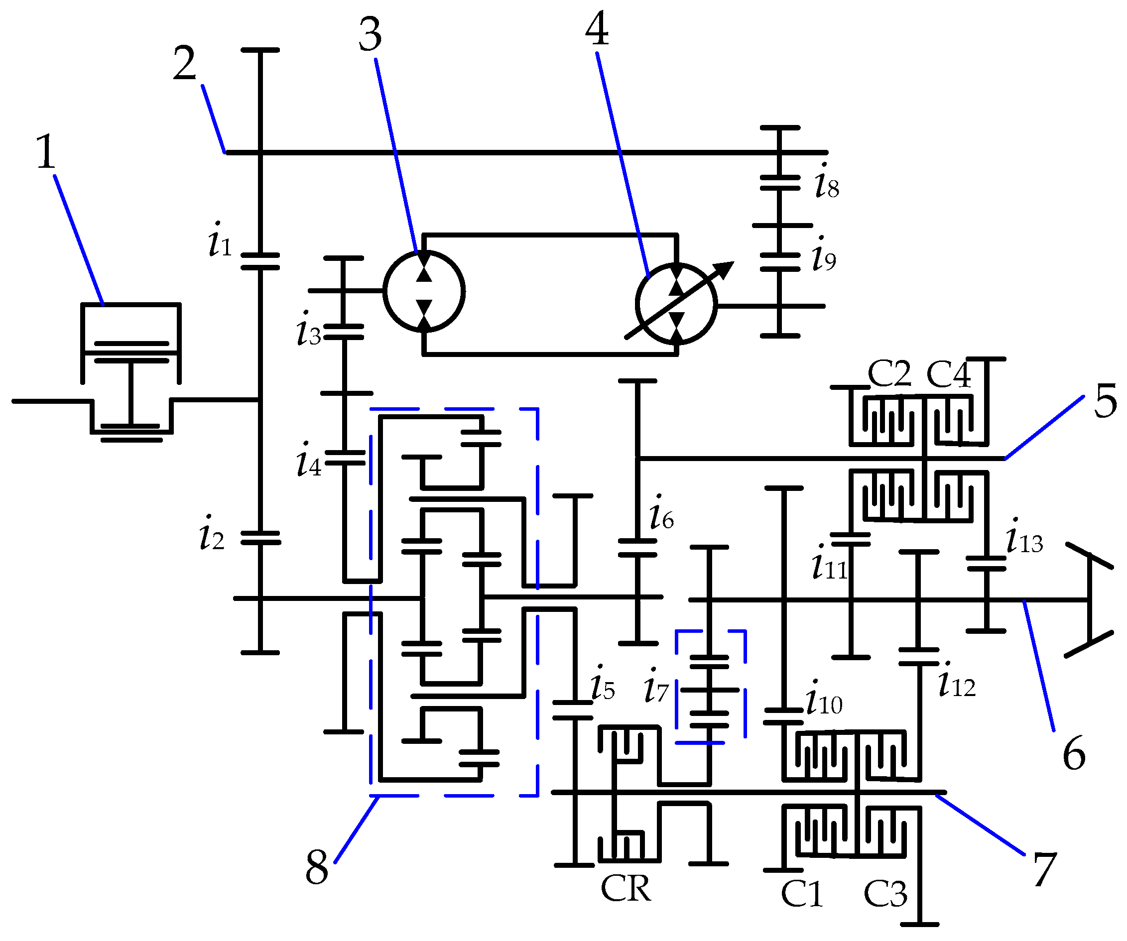
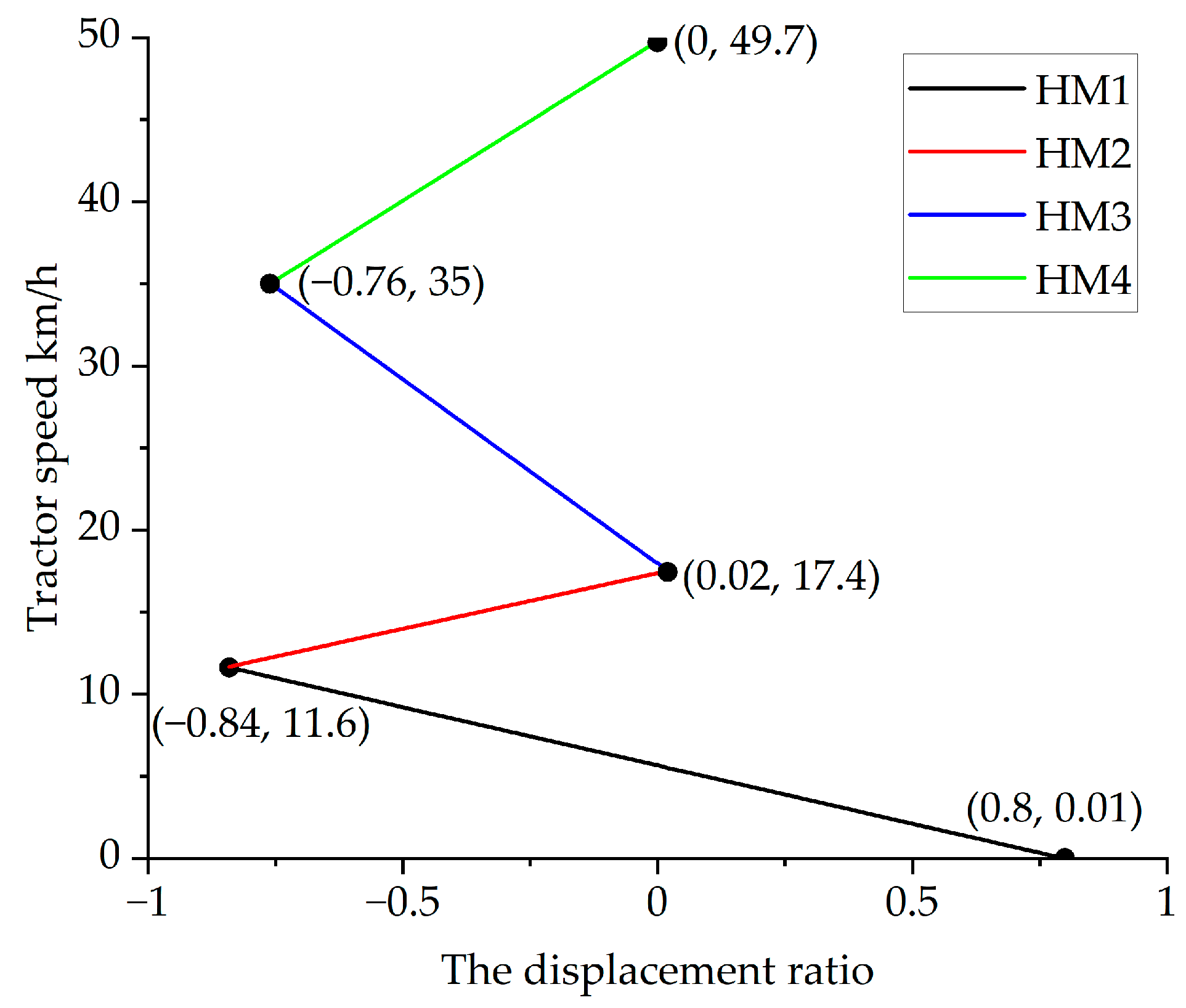
2.1. HMCVT Transmission Principle

This paper is based on an HMCVT composed of a constant motor, a variable pump, planetary gears, wet clutches, and fixed shaft gears. The diagram of the HMCVT is shown in Figure 1. The operating principle is that engine power enters the first intermediate shaft and left sun gear of composite planetary arrangement through i₁ and i₂, respectively. The power entering the first intermediate shaft goes to variable pump through i₈ and i₉, which drives a constant motor. The motor power goes to composite planetary gear ring through i₃ and i₄, and is coupled with left sun gear power before being output, respectively, via planetary carrier and right sun gear. The planet carrier power goes to the second intermediate shaft through i₆, and the sun gear power goes to the third intermediate shaft through i₅. Power enters the output shaft through the clutch and corresponding gear placed on the shaft. CR and i₇, C1 and i₁₀, C2 and i₁₁, C3 and i₁₂, C4 and i₁₃ form reverse gear, forward HM1, forward HM2, forward HM3, and forward HM4, respectively.

As the displacement ratio (the ratio of the actual displacement of the variable displacement pump to the theoretical displacement, −1 to 1) changes, HMCVT can enable tractors to operate at speeds of 0.01 to 49.7 km/h. The forward speed characteristics of HMCVT are shown in Figure 2.

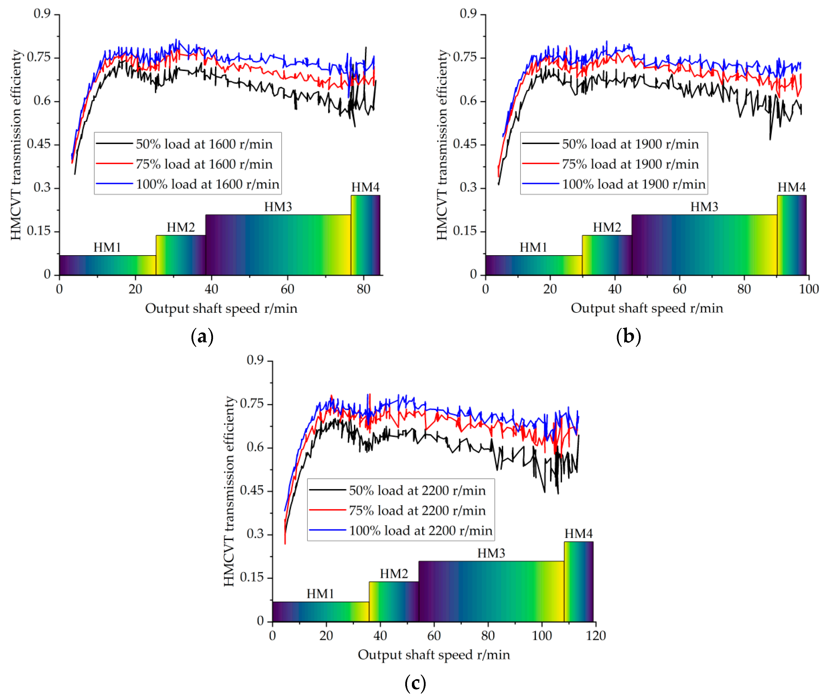
• HM1 segment speed range is 0.01~11.6 km/h, corresponding to a displacement ratio of 0.8~−0.84;
• HM2 segment speed range is 11.6~17.4 km/h, corresponding to a displacement ratio of −0.84~0.02;
• HM3 segment speed range is 17.4~35 km/h, corresponding to a displacement ratio of 0.02~−0.76;
• HM4 segment speed range is 35~49.7 km/h, corresponding to a displacement ratio of −0.76~0.

2.2. Simplified Model of Transmission Efficiency

The transmission efficiency of HMCVT is composed of mechanical and hydraulic efficiency. Mechanical circuit is mainly fixed shaft and planetary gear transmission. The average meshing efficiency η_g of a gear pair is:

$${\eta }_g=1-\pi f(\frac{1}{z_1}\pm \frac{1}{z_2})({\epsilon }_1^2+{\epsilon }_2^2+1-{\epsilon }_1-{\epsilon }_2)$$

(1)

where f is the friction coefficient; z₁ and z₂ are the number of teeth; ε₁ is the ratio of the distance from node to meshing end point to the base pitch; ε₂ is the distance from the meshing starting point to the node.

The transmission efficiency η_p of planetary gear mechanism is:

$${\eta }_p=\frac{P-{\displaystyle \sum _{i=1}^n{L}_i}}{P}$$

(2)

where P is the input power; L_i is the meshing power loss of the gear pair.

Hydraulic circuit is a volume speed-adjusting type composed of a variable pump and a constant motor. The hydraulic efficiency is greatly affected by system parameters (temperature, oil dynamic viscosity, oil density, leakage, etc.), control parameters (swash plate angle) and working conditions (speed and torque), and there are interactions between various factors [22]. It is difficult to use mathematical models to express finely. Ignoring the influence of system parameters, the leakage of pump motor is equivalent to laminar leakage. A simplified efficiency model of variable displacement pump and quantitative motor is:

$${\eta }_{pump}=\frac{1-C_{sp}\frac{\Delta P}{e\mu n_p}}{1+C_{vp}\frac{\mu n_p}{e\Delta P}+\frac{C_{fp}}{e}}$$

(3)

$${\eta }_{motor}=\frac{1-C_{vm}\frac{\mu n_m}{e\Delta P}-C_{fm}}{1+C_{sm}\frac{\mu n_m}{e\Delta P}}$$

(4)

where η_pump and η_motor are variable pump and quantitative motor efficiency, respectively; e is the displacement ratio of variable pump; C_sp, C_vp and C_fp are the laminar leakage coefficient, laminar resistance coefficient and mechanical resistance coefficient of the variable pump, respectively; ΔP is the pressure drop of hydraulic circuit; μ is the dynamic viscosity of hydraulic oil; C_sm, C_vm and C_fm are the laminar leakage coefficient, laminar resistance coefficient and mechanical resistance coefficient of the constant motor, respectively.

Therefore, the transmission efficiency of the whole HMCVT can be expressed as:

$${\eta }_{HMCVT}={\eta }_g^i{\eta }_p{\eta }_{pump}{\eta }_{motor}$$

(5)

where ${\eta }_g^i$ is the total transmission efficiency of the fixed shaft gear pair of HM_i.

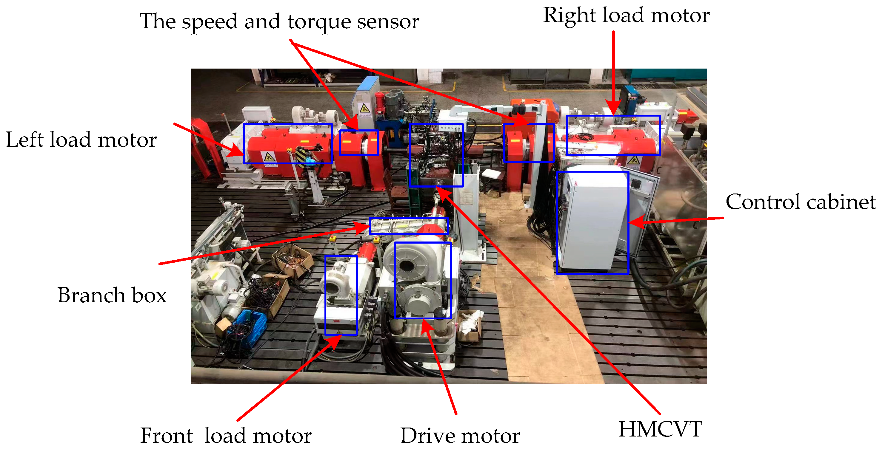
2.3. HMCVT Test Bench

The test bench consists of a drive motor, loading motors (front drive shaft, left and right semi-axle loading motors), a branch box, torque sensors, oil pressure sensors, HMCVT and a control cabinet, as shown in Figure 3.

The driving motor is a 340 kW AC variable frequency motor (rated torque 1910 Nm, maximum speed 3000 r/min, moment of inertia 1.5 kgm²) from AKH (Antriebstechnik KATT Hessen GmbH, Homberg, Germany). The front, left, and right semi-axle loading motors are, res, if yes, please addpectively, 125 kW (rated torque 1400 Nm, maximum speed 1600 r/min, moment of inertia 1.5 kgm²), 165 kW (rated torque 3500 Nm, maximum speed 2700 r/min, moment of inertia 5.6 kgm²), and 165 kW (rated torque 3500 Nm, maximum speed 2700 r/min, moment of inertia 5.6 kgm²) AC variable frequency motors from AKH (Antriebstechnik KATT Hessen GmbH, Homberg, Germany). The torque sensors are T10FS from HBM (Hottinger Brüel & Kjaer GmbH, Darmstadt, Germany), and the accuracy is ±0.5% F.S (the range of torque sensor between the driving motor and HMCVT is 0~2 kNm, which between the front drive loading motor and branch box is 0~2 kNm, and which between the left semi-axle, right semi-axle, and HMCVT is 0~50 kNm). The rated input speed of HMCVT is 2200 r/min, the rated input torque is 735 Nm, and the rated input power is 169 kW. The oil pressure sensor is a UNIK500 pressure transmitter from DRUCK (Baker Hughes Co., Ltd., Houston, TX, USA), with a range of 0~3 MPa and an accuracy of ±0.5% F.S.

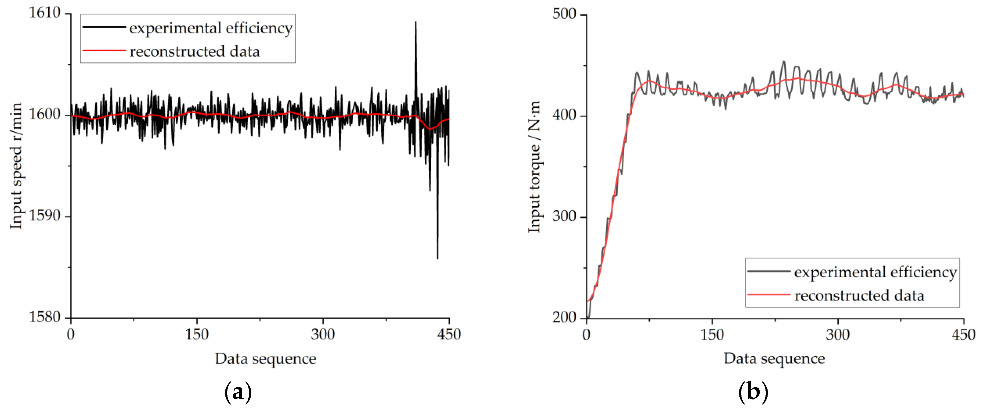
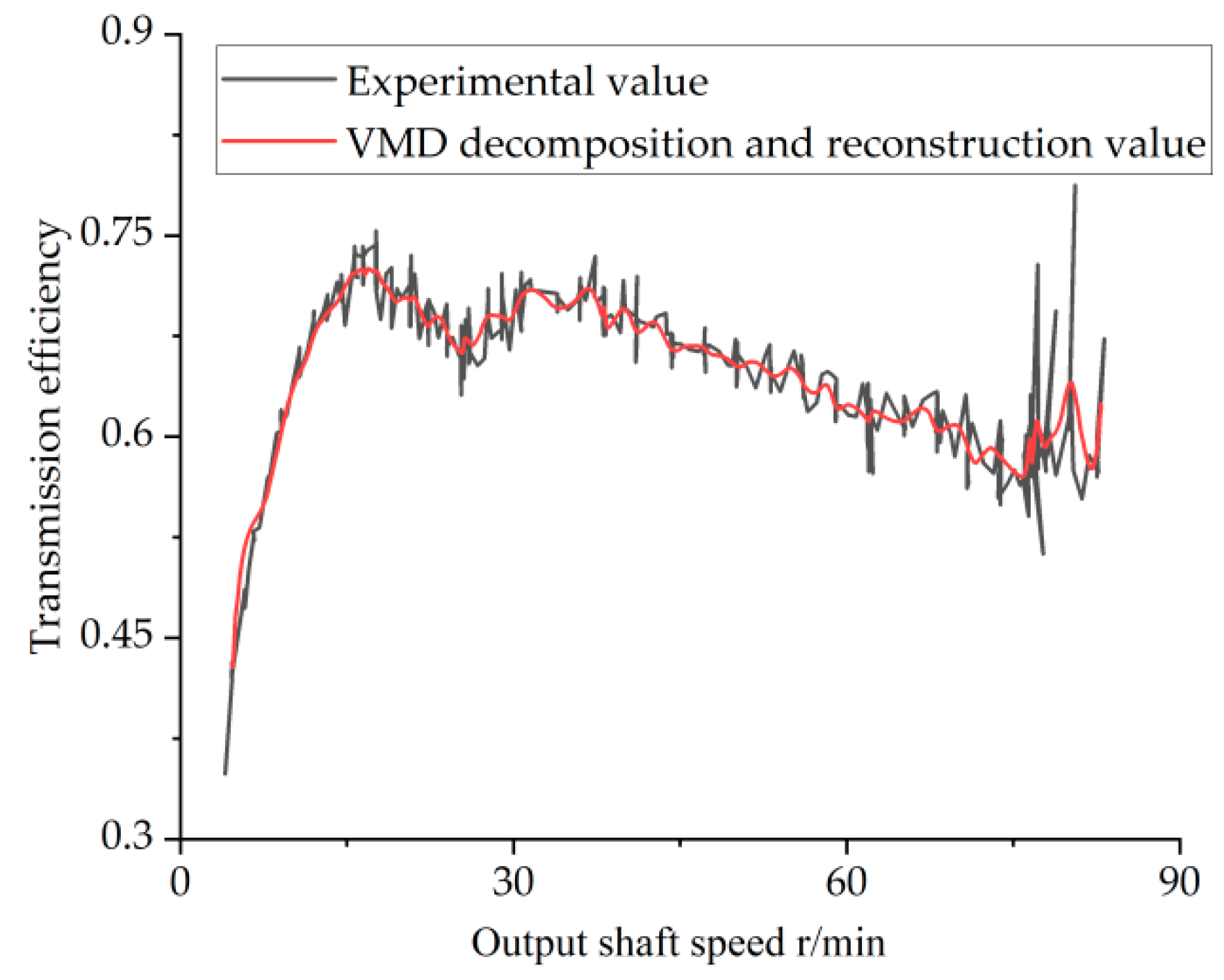
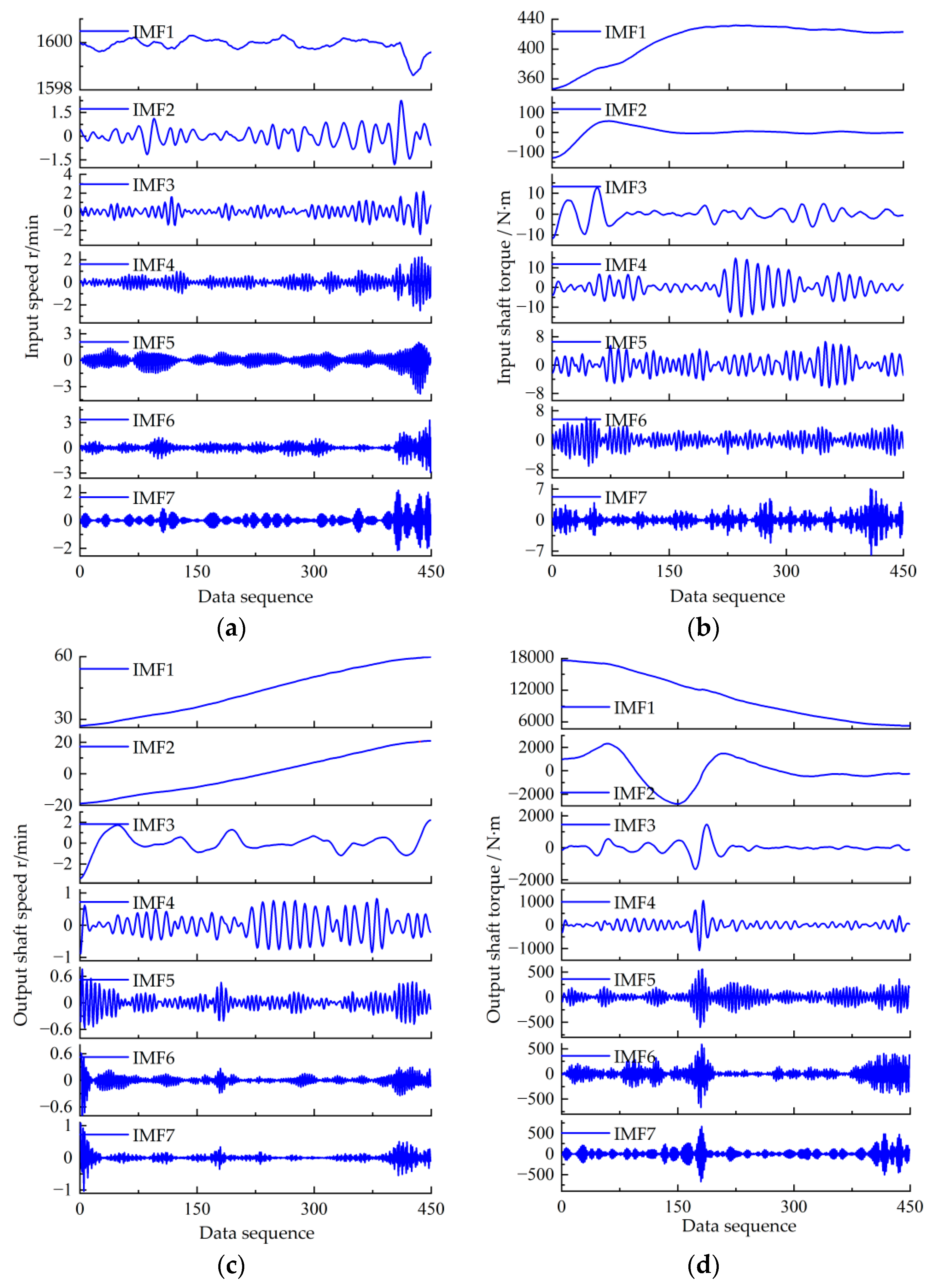
2.4. Data Denoising Method Based on VMD

VMD is a completely non-recursive, adaptive computing bandwidth data decomposition algorithm proposed by Dragomiretskiy et al. [23]. VMD applies Wiener filter to the residual estimation of the effective intrinsic mode function (IMF) component, allowing for online updating of the center frequency in Fourier domain. Therefore, it has strong robustness to sampling and noise, and is widely used in signal denoising [24,25,26,27]. In the transmission efficiency test data denoising problem, VMD firstly decomposes the collected signal into multiple discrete IMF components. Then, Hilbert transform is used to obtain a unilateral spectrum of each IMF component, and then unilateral spectrum is exponentially mixed with the estimated center frequency to obtain the baseband of each IMF. Finally, the Gaussian smoothness is used to demodulate the IMF component bandwidth, accordingly, the signal decomposition is transformed into a constrained variational problem. The variational problem is defined as:

$$\underset{\left\{u_k\right\}, \left\{{\omega }_k\right\}}{\min }\left\{{{\displaystyle \sum _k‖{\partial }_t\left[\left(\delta \left(t\right)+\frac{j}{\pi t}\right)\ast u_k(t)\right]e^{-j{\omega }_{k}t}‖}}_2^2\right\}\hspace{1em}\hspace{1em}s.t. {\displaystyle \sum _k{u}_k=f_1}$$

(6)

where u_k is IMF components of the signal f₁ to be decomposed; ω_k is center frequency of each IMF component.

To solve the variational problem, the Lagrangian multiplier λ and a quadratic penalty factor α are introduced to transform the constrained variational problem into unconstrained. The augmented Lagrangian function obtained is:

$$\begin{array}{l}L\left(\left\{u_k\right\}, \left\{{\omega }_k\right\}, \lambda \right)=\alpha {{\displaystyle \sum _k‖{\partial }_t\left[\left(\delta \left(t\right)+\frac{j}{\pi t}\right)\ast u_k(t)\right]e^{-j{\omega }_{k}t}‖}}_2^2\\ +{‖f(t)-{\displaystyle \sum _k{u}_k(t)}‖}_2^2+〈\lambda (t), f\left(\mathrm{t}\right)-{\displaystyle \sum _k{u}_k(t)}〉\end{array}$$

(7)

Then, the Alternating Direction Method of Multipliers (ADMM) is used to calculate the saddle points of the augmented Lagrangian function, and u_k, ω_k and λ are iteratively updated in frequency domain in real-time. Thus, each IMF component and its corresponding center frequency are calculated. The updated formula for u_k is:

$${\widehat{u}}_k^{n+1}(\omega )=\frac{\widehat{f}(\omega )-{\displaystyle \sum _{i<k}{{\widehat{u}}_i}^{n+1}(\omega )}-{\displaystyle \sum _{i>k}{{\widehat{u}}_i}^n(\omega )+\frac{{\widehat{\lambda }}^n(\omega )}{2}}}{1+2\alpha {(\omega -{\omega }_k^n)}^2}$$

(8)

The updated formula for ω_k is:

$${\omega }_k^{n+1}=\frac{{\displaystyle {\int }_0^{\infty }\omega {\left|{\widehat{u}}_k^{n+1}(\omega )\right|}^2\mathrm{d}\omega }}{{\displaystyle {\int }_0^{\infty }{\left|{\widehat{u}}_k^{n+1}(\omega )\right|}^2\mathrm{d}\omega }}$$

(9)

The updated formula for λ is:

$${\widehat{\lambda }}^{n+1}(\omega )={\widehat{\lambda }}^n(\omega )+\tau (\widehat{f}(\omega )-{\displaystyle \sum _k{{\widehat{u}}_i}^{n+1}(\omega )})$$

(10)

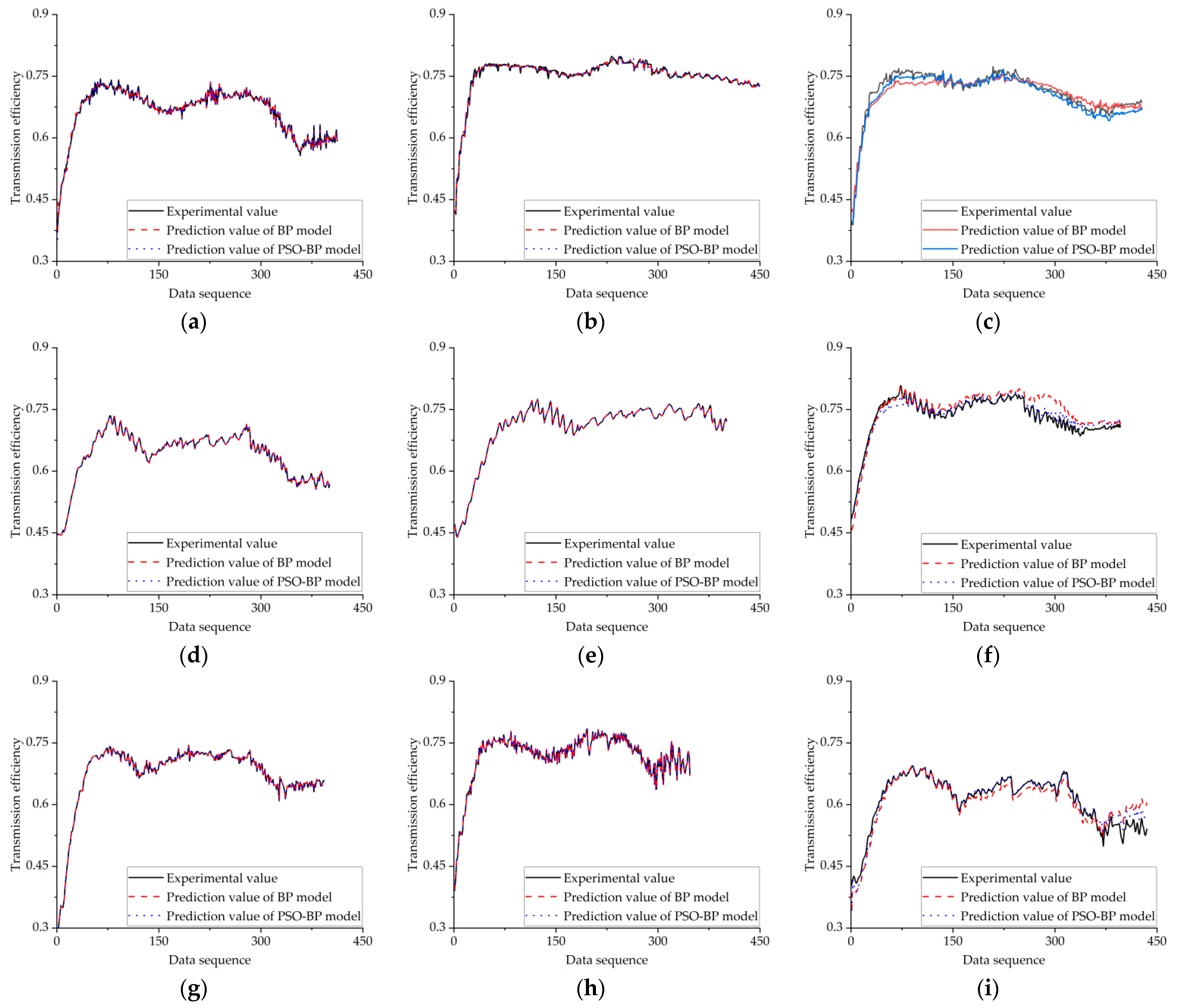
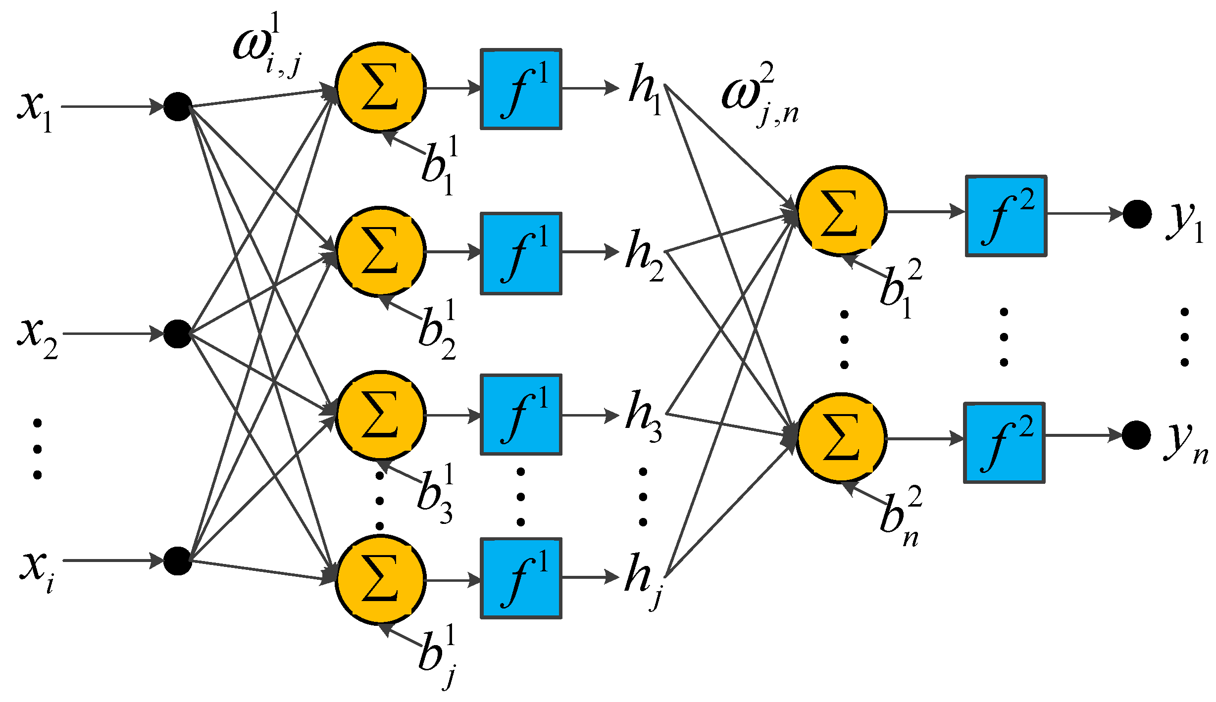
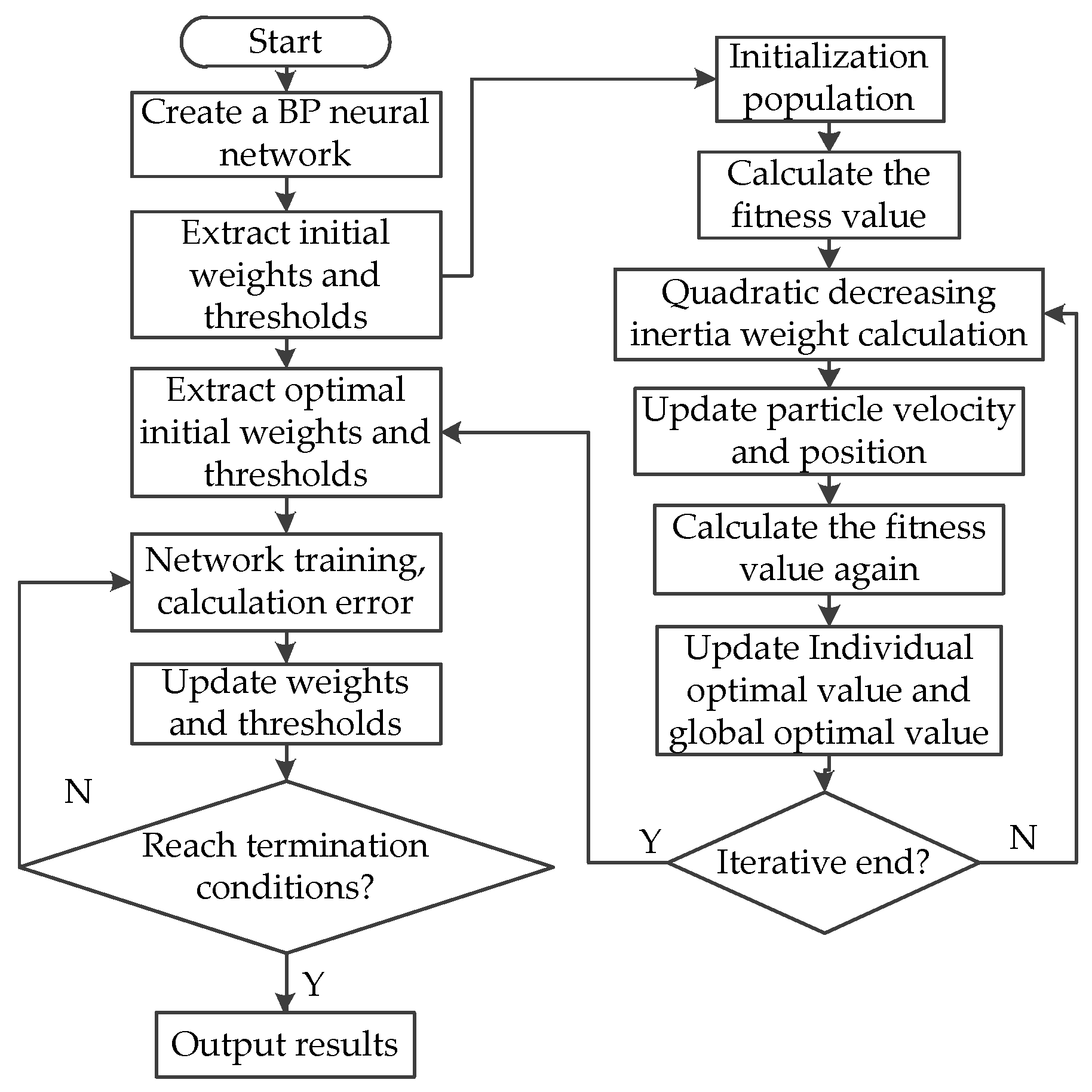
2.5. Transmission Efficiency Prediction Model Based on PSO–BP

BP neural network is a typical multi-layer feed-forward network with error back propagation ability. It has the advantages of simple structure, fast calculation speed, and high stability, and only needs 3 layers to approximate any nonlinear continuous function. Therefore, the BP neural network is widely used in various prediction and classification fields. A typical 3-layer BP neural network structure is shown in Figure 4.

For a 3-layer BP neural network with i input nodes, j hidden nodes and n output nodes, the output value of any node in hidden layer is:

$$h_j=f^1({\displaystyle \sum _{m=1}^i{x}_m{\omega }_{m,j}+b_j^1})$$

(11)

where f¹ is the activation function from input layer to hidden layer; x_m is the m-th input, m = 1, 2, …, i; ω_m,j is the weight coefficient of the m-th input and the j-th node of hidden layer; $b_j^1$ is the threshold value of the j-th node.

The output value of any node in output layer is:

$$y_n=f^2({\displaystyle \sum _{t=1}^j{h}_t{\omega }_{t,n}+b_n^2})$$

(12)

where f² is the activation function from hidden layer to output layer;. ω_t,n is the weight coefficient of the t-th node and the n-th node; $b_n^2$ is the threshold value of the n-th node.

BP neural network uses the gradient descent method to continuously renew the weights and thresholds along the negative gradient direction of model error until the model error reaches antecedent requirements. The weight update formula is:

$$\left\{\begin{array}{l}{\omega }_{m,j}(k+1)={\omega }_{m,j}(k)+\mu h_t(1-h_t)x_m{\displaystyle \sum _{m=1}^i{\omega }_{j,t}{e}_t}\hfill \\ {\omega }_{j,n}(k+1)={\omega }_{j,n}(k)+\mu h_t{e}_t\hfill \end{array}\right.$$

(13)

where k is the times of updates of the weights; μ is the learning rate; e_t is the model error.

The threshold update method is:

$$\left\{\begin{array}{l}{b}_j^1(k+1)=b_j^1(k)+h_t(1-h_t){\displaystyle \sum _{m=1}^i{\omega }_{j,t}{e}_t}\hfill \\ b_n^2(k+1)=b_n^2(k)+e_t\hfill \end{array}\right.$$

(14)

The training speed and accuracy of BP neural network are greatly affected by the initial weights and thresholds. Therefore, a PSO algorithm is used to optimize the weights and thresholds. The PSO algorithm has the advantages of fast convergence speed, fewer parameters, and simple and easy implementation. However, the standard PSO algorithm has problems of premature convergence and late time oscillation. By introducing a quadratic decreasing inertia weight, the algorithm can enhance the global search ability with a larger inertia in the early stage, and obtain better later local optimization ability with a smaller inertia weight. The improved PSO particle velocity and position update formula is:

$$\left\{\begin{array}{l}v(t+1)={\omega }_{n}v(t)+c_1{r}_1\left[p_{best}-x(t)\right]+c_2{r}_2\left[g_{best}-x(t)\right]\\ x(t+1)=x(t)+v(t+1)\\ {\omega }_n={\omega }_{\max }-\frac{({\omega }_{\max }-{\omega }_{\min })}{T^2}{t}^2\end{array}\right.$$

(15)

where v is the particle moving speed; ω_n is the quadratic decreasing inertia weight; c₁ is the individual learning factor; c₂ is the global learning factor; r₁ and r₂ are random numbers uniformly distributed between [0, 1]; x is the particle position; p_best is the optimal solution of particle individual; g_best is the global optimal solution of particle; ω_max is the maximum inertia weight; ω_min is the minimum inertia weight; T is the total times of iterations; t is the current times of iterations.

The algorithm flow of PSO optimizing BP neural network is shown in Figure 5. Firstly, a BP neural network structure was model created and parameters were initialize. Then, extracting initialization weights and thresholds and initialize PSO parameters. And then, velocity and position of all particles in the population were updated by quadratic decreasing weight, and the fitness was calculated again. When the iteration termination condition was satisfied, the optimal weights and thresholds were assigned to the BP neural network. Finally, the assigned BP neural network would be trained.

2.6. Analysis of the Importance of Factors on the Transmission Efficiency Based on PLS

PLS combines multiple linear regression, canonical correlation analysis, and principal component analysis. In addition, PLS can better explain the impact of each independent variable [28,29]. In order to quantitatively analyze the importance of input speed, power and output speed to HMCVT transmission efficiency, this paper uses PLS to analyze the test data.

3. Results and Discussion

3.1. Transmission Efficiency Characteristics of HMCVT

The HMCVT transmission efficiency was tested by a constant power loading mode. The driving motor speed was set to 1600, 1900, and 2200 r/min, respectively. The loading power is 50%, 75% and 100% of the maximum power of the engine matched by HMCVT at the corresponding input speed, respectively. At a certain input speed and power, the transmission ratio continuous change was realized within the design range by cooperatively controlling the clutch, synchronizer, and variable pump displacement ratio. Then, the transmission efficiency within the whole transmission ratio range under this working condition was measured. The signals collected during the test were the input speed and torque, as well as the output speed and torque. The transmission efficiency was expressed as the ratio of the product of output speed and torque to the input. During the test, the relationship between the transmission efficiency of the HMCVT and the output shaft speed is shown in Figure 6.

In Figure 6, the more obvious regularity is that under coincident input speed and power, the transmission efficiency increases first and then decreases in the HM1 segment, continues to rise in the HM2 segment, continues to decline in the HM3 segment, and rises slightly in the HM4 segment. The main reason for this regularity is that the proportion of hydraulic circuit power to the total output power changes. The displacement ratio of the HM1 segment changes from 0.8 to −0.84. In this process, the power ratio of the hydraulic circuit decreases to 0 and then increases. Due to the low transmission efficiency of the hydraulic circuit, HMCVT transmission efficiency increases first and then decreases. Identically, the displacement ratio of the HM2 segment changes from −0.84 to 0.02 and the HM3 segment changes from 0.02 to −0.76, which changes the power ratio of the hydraulic circuit, making an HMCVT transmission efficiency alteration. The power ratio of the HM4 segment of the hydraulic circuit decreases gradually, which makes the HMCVT transmission efficiency increase again. The final performance is that the HMCVT transmission efficiency changes significantly with an increase in output speed, and reaches a maximum value when the displacement ratio of the HM1 segment is 0, and then shows a downward trend as a whole. Furthermore, the transmission efficiency is positively correlated with load and negatively correlated with input speed.

Ulteriorly, we analyzed the impact of the working conditions on transmission efficiency. The PLS method was used to evaluate the importance of input speed, power, and output speed on transmission efficiency. The contributions of these three factors to transmission efficiency were 0.54, 1.12, and 1.21, respectively. This indicates that output shaft speed has the greatest impact on transmission efficiency, followed by power, and the input speed has the smallest impact. Therefore, in the prediction of transmission efficiency, the weight of the power and the output speed should be appropriately considered, and the weight of the input speed should be weakened.

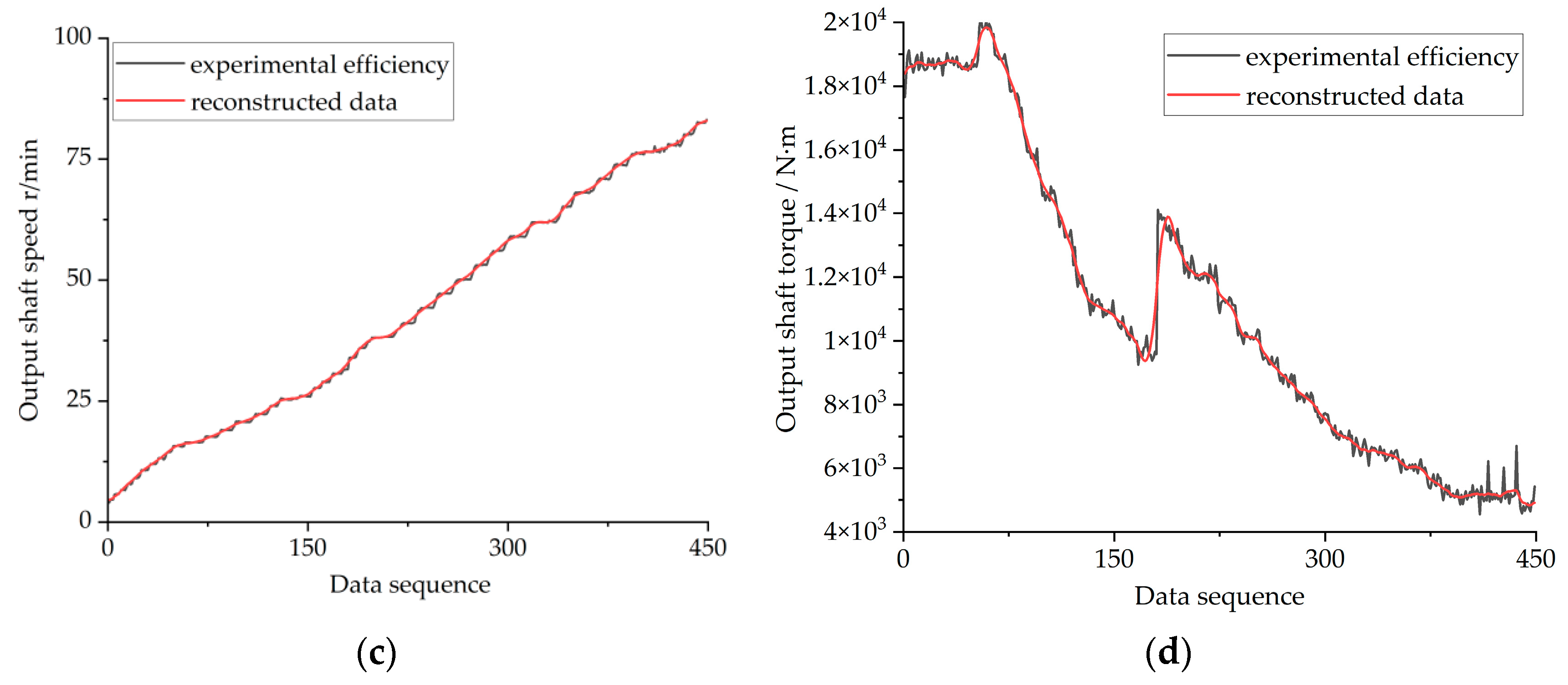
3.2. Denoising Results and Analysis of Test Data Based on VMD

Taking 1600 r/min with 100% load condition as an example, the collected input shaft speed, torque and output shaft speed, and torque signals were decomposed by VMD to improve the signal-to-noise ratio. The value of α in the VMD model is 2000, and the number of modal components K is 7. The results of VMD decomposition are shown in Figure 7.

According to the results, VMD decomposed the speed and torque signals into seven IMF components, and adaptively calculated the center frequency and bandwidth of each IMF component. Among the seven decomposed IMF components, principal components with larger amplitudes and longer periods can be regarded as effective signals, while the principal components with smaller amplitudes and shorter periods can be regarded as noise signals. Therefore, the input speed signal is reconstructed by the IMF1 component, the input torque is reconstructed by the IMF1 and IMF2 components, and the output speed and output torque are reconstructed by the IMF1, IMF2 and IMF3 components. The comparison between the reconstructed data and the original data is shown in Figure 8.

Based on Figure 8, the data reconstructed without short period and small amplitude IMF components has better flatness while retaining the characteristics of the original data signal, indicating that the VMD algorithm can accurately extract the effective signal and noise signal. Apparently, the reconstructed data can truly reflect the feature information of the original data and has a higher signal-to-noise ratio. The transmission efficiency recalculated using the reconstructed data is shown in Figure 9.

The recalculated transmission efficiency curve eliminates the peaks and valleys existing in the original data, making the curve smoother, and reflecting the value and trend of actual HMCVT transmission efficiency. Obviously, the difficulty of transmission efficiency prediction was reduced to some degree.

3.3. Transmission Efficiency Prediction Results and Analysis

In accordance with Equation (5), HMCVT transmission efficiency is determined by transmission route and hydraulic circuit efficiency. The transmission route of HMCVT is determined by the segment. According to Equations (3) and (4), ignoring the parameters effect, the hydraulic circuit efficiency is mainly decided by the displacement ratio, the pressure difference of the hydraulic circuit, and the speed of the pump motor. Evidently, the displacement ratio and speed of the pump motor can be calculated by the input speed and output speed, and the pressure difference of the hydraulic circuit is positively correlated with the output torque. Therefore, the input variables of the prediction model are set as the segment, input speed, and torque decomposed by the VMD, and the output speed and torque. At the same time, the output variable is transmission efficiency. Meanwhile, in order to avoid the influence of data magnitude on prediction accuracy, the input and output variables are normalized, and the normalized interval is [0, 1]. Finally, in order to show the feasibility of transmission efficiency prediction and the prediction effect of the PSO–BP model, a training set and a test set are created. The training set includes experimental data under 50% and 70% loads at 1600 r/min, 50% and 75% loads at 1900 r/min, and 75% and 100% loads at 2200 r/min. The test set includes data under 75% load at 1600 r/min, 100% load at 1900 r/min, and 50% load at 2200 r/min. The training and test results are shown in Figure 10.

As shown in Figure 10, both the BP and the PSO–BP model can achieve an accurate prediction of the training data set, indicating that it is feasible to predict the transmission efficiency of HMCVT. More importantly, the prediction results of the test set data show that the performance of the PSO–BP model is better than that of the BP neural network. The regression performance is as follows: the fitting R² of the PSO–BP model for the prediction results of 75% load at 1600 r/min, 100% load at 1900 r/min, and 50% load at 2200 r/min are 0.930, 0.945, and 0.968, respectively, which were 7.02%, 7.88% and 9.26% higher than that of the BP neural network.

In order to deeply compare the BP and the PSO–BP models, the mean absolute error (MAE), mean absolute percentage error (MAPE), and root mean square error (RMSE) between the predicted results and experimental data were used to evaluate the prediction effect. Moreover, so as to avoid the influence of random factors on the results, three prediction tests were carried out on the three working conditions using two models. The results are shown in

Table 1. Transmission efficiency prediction test results.

Working Conditions	Type of Error	Model	Prediction Error Value			Error Mean
			1	2	3
75% load at 1600 r/min	MAE	BP	0.013	0.017	0.014	0.015
		PSO–BP	0.012	0.010	0.012	0.011
	MAPE/%	BP	1.969	2.366	1.985	2.107
		PSO–BP	1.370	1.812	1.809	1.664
	RMSE	BP	0.020	0.021	0.019	0.020
		PSO–BP	0.015	0.012	0.016	0.014
100% load at 1900 r/min	MAE	BP	0.014	0.017	0.014	0.015
		PSO–BP	0.009	0.011	0.009	0.010
	MAPE/%	BP	2.018	2.393	1.940	2.117
		PSO–BP	1.239	1.443	1.214	1.299
	RMSE	BP	0.019	0.020	0.015	0.018
		PSO–BP	0.010	0.011	0.010	0.010
50% load at 2200 r/min	MAE	BP	0.019	0.011	0.016	0.015
		PSO–BP	0.008	0.009	0.008	0.008
	MAPE/%	BP	3.116	1.857	2.843	2.605
		PSO–BP	1.519	1.056	1.363	1.313
	RMSE	BP	0.024	0.017	0.021	0.021
		PSO–BP	0.013	0.009	0.011	0.011

.

As shown in Table 1, the mean values of MAE, MAPE, and RMSE of the PSO–BP model under the three working conditions are smaller than those of the BP. Among them, the mean values of MAE, MAPE, and RMSE of the PSO–BP model are mostly reduced by 46.7%, 49.6%, and 47.6%, respectively, compared with the BP, which are generated at a 50% load condition of 2200 r/min. This shows that the accuracy of the PSO–BP model in predicting transmission efficiency is better than that of BP. Additionally, the maximum differences of the three error types in the prediction results of the PSO–BP model are 0.002, 0.463%, and 0.004, respectively, which are 0.006, 0.796%, and 0.003 lower than those of BP, respectively. It evidences that the PSO–BP model is more stable than the BP model.

In summary, from the statistical results of efficiency prediction, the accuracy and stability of the PSO–BP model in predicting transmission efficiency are better than those of BP.

4. Conclusions

Based on the HMCVT test bench, we carried out a multi-condition transmission efficiency test. The experimental data showed that the alteration of the hydraulic power proportion was the main reason for the change in overall HMCVT transmission efficiency. With an increase in output speed, the efficiency of HMCVT reached the maximum when the displacement ratio of the HM1 segment was 0, and then presented a downward trend as a whole. The transmission efficiency was positively correlated with load and negatively correlated with input speed. PLS analysis showed that the output shaft speed had the greatest influence on the transmission efficiency, followed by the power, and the input speed had the least influence.

Furthermore, we decomposed and reconstructed the transmission efficiency experimental data based on the VMD algorithm. The results show that the VMD algorithm decomposed the original transmission efficiency data into multiple IMF components of effective signal and noise signal, respectively. The reconstructed data based on effective signal IMF components preserved the original data characteristics, which made the transmission efficiency smoother and reduced the difficulty of prediction.

Moreover, a transmission efficiency prediction model was established using a BP neural network, and the parameters of the BP neural network were optimized using the PSO algorithm. The prediction results of transmission efficiency indicated that the R² of the POS–BP model for predicting transmission efficiency under three working conditions were 0.930, 0.945, and 0.968, respectively, which were 7.02%, 7.88%, and 9.26% higher than the regression accuracy of the BP neural network. The maximum differences in MAE, MAPE, and RMSE of the PSO–BP model were 0.002, 0.463%, and 0.004, respectively, which were reduced by 0.006, 0.796%, and 0.003 compared to the BP neural network. The accuracy and stability of the PSO–BP model in predicting transmission efficiency are better than those of the BP neural network for statistical significance.

References

1. Xie, B.; Wu, Z.B.; Mao, E.R. Development and prospect of key technologies on agricultural tractor. Trans. Chin. Soc. Agric. Mach. 2018, 49, 1–17. [Google Scholar]
2. Lu, K.; Lu, Z.X. Analysis of HMCVT shift quality based on the engagement characteristics of wet clutch. Agriculture 2022, 12, 2012. [Google Scholar] [CrossRef]
3. Lu, K.; Lu, Y.; Deng, X.T.; Wang, L.; Zhao, Y.R.; Lu, Z.X. Torque handover and control of the HMCVT shift clutches under the theoretical shift condition. Trans. Chin. Soc. Agric. Eng. 2023, 38, 23–32. [Google Scholar]
4. Lu, K.; Wang, L.; Lu, Z.X.; Zhou, H.D.; Qian, J.; Zhao, Y.R. Sliddng mode control for HMCVT shifting clutch pressure tracking based on expanded observer. Trans. Chin. Soc. Agric. Mach. 2022, 54, 410–418. [Google Scholar]
5. Linares, P.; Méndez, V.; Catalán, H. Design parameters for continuously variable power-split transmissions using planetaries with 3 active shafts. J. Terramech. 2010, 47, 325–335. [Google Scholar] [CrossRef]
6. Yu, J.; Dong, X.H.; Song, Y.R. Energy efficiency optimization of a compound coupled hydro-mechanical transmission for heavy-duty vehicles. Energy 2022, 252, 123937. [Google Scholar] [CrossRef]
7. Wang, C. Determination of power flow and calculation of transmission efficiency for 2K-H closed epicyclic gear train. J. Mech. Eng. 2023, 59, 59–67. [Google Scholar]
8. Wang, W.J.; Yang, G.L.; Du, Q.H.; Chen, Q.Y. Design of 3K planetary gear reducer with no backlash. Chin. Mech. Eng. 2024, 35, 36–44. [Google Scholar]
9. Cui, L.; Qin, D.T.; Shi, W.K. Reference efficiency of planetary gear train. J. Chongqing Univ. Nat. Sci. Ed. 2006, 29, 11–14. [Google Scholar]
10. Geng, B.L.; Gu, L.C.; Liu, J.M. Novel methods for modeling and online measurement of effective bulk modulus of flowing oil. IEEE Access 2020, 8, 20805–20817. [Google Scholar] [CrossRef]
11. Xu, R.; Gu, L.C. Semi-empirical Parametric modeling for efficiency characteristics of axial piston pump. Trans. Chin. Soc. Agric. Mach. 2016, 47, 382–390. [Google Scholar]
12. İnce, E.; Güler, M.A. On the advantages of the new power-split infinitely variable transmission over conventional mechanical transmissions based on fuel consumption analysis. J. Cleaner Prod. 2020, 244, 118795. [Google Scholar] [CrossRef]
13. Huang, X.K.; Lu, Z.X.; Qian, J.; An, Y.H. Optimization of tractor HMCVT target speed ratio and control simulation based on machine economy. J. Nanjing Agric. Univ. 2022, 45, 777–787. [Google Scholar]
14. Zhang, M.Z.; Wang, J.Z.; Wang, J.H.; Guo, Z.Z.; Guo, F.Q.; Xi, Z.Q.; Xu, J.J. Speed changing control strategy for improving tractor fuel economy. Trans. Chin. Soc. Agric. Eng. 2020, 36, 82–89. [Google Scholar]
15. Blake, C.; Monika, I.; Kyle, W. Comparison of Operational Characteristics in Power Split Continuously Variable Transmissions. In Proceedings of the Commercial Vehicle Engineering Congress and Exhibition, Chicago, IL, USA, 31 October 2006. [Google Scholar]
16. Zhang, G.Q.; Wang, K.X.; Xiao, M.H.; Zhou, M.H. HMCVT steady state transmission efficiency based on HST-EGT torque ratio. Trans. Chin. Soc. Agric. Mach. 2021, 52, 533–541. [Google Scholar]
17. Liang, L.; Li, Q.T.; Tan, Y.Y.; Yang, Z.H. Multi-parameter optimization of HMCVT fuel economy using parameter cyclic aigorithm. Trans. Chin. Soc. Agric. Eng. 2023, 39, 48–55. [Google Scholar]
18. Wang, G.M.; Zhu, S.H.; Shi, L.X.; Ni, X.D.; Ruan, W.S.; Ouyang, D.Y. Simulation and experiment on efficiency characteristics of hydraulic mechanical continuously variable transmission for tractor. Trans. Chin. Soc. Agric. Eng. 2013, 15, 42–48. [Google Scholar]
19. Zhu, Z.; Gao, X.; Cao, L.L.; Pan, D.Y.; Zhu, Y.; Guo, J. Research on response characteristic and efficiency characteristic of pump-control-motor system. Mach. Tool Hdy. 2016, 44, 87–92. [Google Scholar]
20. Cheng, Z.; Lu, Z.X.; Qian, J. A new non-geometric transmission parameter optimization design method. Comput. Electron. Agric. 2019, 167, 105034. [Google Scholar] [CrossRef]
21. Cheng, Z.; Lu, Z.X. Model modification and parameter identification of tractor hydraulic transmission system characteristics. Trans. Chin. Soc. Agric. Eng. 2023, 38, 33–41. [Google Scholar]
22. Cheng, Z.; Xing, J.; Li, W.J. Efficiency modeling and reducer ratio analysis of hydrostatic transmission system for agricultural and forestry machinery. J. Mech. Electr. Eng. 2024, 41, 99–106. [Google Scholar]
23. Dragomiretskiy, K.; Zosso, D. Variational Mode Decomposition. IEEE Trans. Signal. Process. 2014, 62, 531–544. [Google Scholar] [CrossRef]
24. Liu, B.X.; Zhang, Y.M.; Jiang, Z. Noise reduction method of pipeline leakage signal based on variational mode decomposition. J. Vibra. Meas. Diagn. 2023, 43, 397–403. [Google Scholar]
25. Gao, H.T.; Kang, J.H.; Zhang, Z.; Wu, B. Enhancement of signal-to-noise ratio based on variational mode decomposition for phase-sensitive optical time domain reflectometry. Acta Opt. Sin. 2023, 43, 49–58. [Google Scholar]
26. Li, B.; Li, X.; Rui, H.; Liang, Y. Displacement prediction of tunnel entrance slope based on variational modal decomposition and grey wolf optimized extreme learning machine. J. Jilin Univ. Eng. Technol. Ed. 2023, 53, 1853–1860. [Google Scholar]
27. Wang, J.H.; Li, H.G.; Zhang, W.D.; Chen, Y.N. Adaptive modal total variational mode decomposition method and its performance evaluation. J. Vibr. Shock 2023, 42, 251–262. [Google Scholar]
28. Xia, L. Analysis of partial least squares modeling and multi-collinearity ability. Agro Food Ind. Hi-Tech 2017, 28, 885–889. [Google Scholar]
29. Xu, Q.S.; Liang, Y.Z.; Shen, H.L. Generalized PLS regression. J. Chemom. 2001, 15, 135–148. [Google Scholar] [CrossRef]
Figure 1. The diagram of HMCVT. Note: 1—engine; 2—the first intermediate shaft; 3—constant motor; 4—variable pump; 5—the second intermediate shaft; 6—output shaft; 7—the third intermediate shaft; 8—composite planetary arrangement.
Agriculture 14 00539 g001
Figure 2. HMCVT forward speed characteristics.
Agriculture 14 00539 g002
Figure 3. Physical diagram of HMCVT test bench.
Agriculture 14 00539 g003
Figure 4. A 3-layer BP neural network structure diagram.
Agriculture 14 00539 g004
Figure 5. PSO optimizes BP neural network algorithm flow.
Agriculture 14 00539 g005
Figure 6. The HMCVT transmission efficiency test results: (a) the transmission efficiency of 1600 r/min; (b) the transmission efficiency of 1600 r/min; (c) the transmission efficiency of 1600 r/min.
Agriculture 14 00539 g006
Figure 7. The VMD decomposition results: (a) input speed decomposition results; (b) input torque decomposition results; (c) output speed decomposition results; (d) output torque decomposition results.
Agriculture 14 00539 g007
Figure 8. The comparison results between the reconstructed and the original data: (a) input speed; (b) input torque; (c) output speed; (d) output torque.
Agriculture 14 00539 g008aAgriculture 14 00539 g008b
Figure 9. Recalculated transmission efficiency.
Agriculture 14 00539 g009
Figure 10. HMCVT transmission efficiency prediction results: (a) 1600 r/min, 50% load training results; (b) 1600 r/min, 100% load training results; (c) 1600 r/min, 75% load test results; (d) 1900 r/min, 50% load training results; (e) 1900 r/min, 75% load training results; (f) 1900 r/min, 100% load test results; (g) 2200 r/min, 75% load training results; (h) 2200 r/min, 100% load training results; (i) 1600 r/min, 50% load test results.
Agriculture 14 00539 g010