1. Introduction
The temperature variable stands out as one of the atmospheric parameters with the highest accuracy, contributing to enhanced reliability in weather forecasts. Precisely predicting the air temperature at a specific location and time is a crucial research challenge with diverse applications, spanning from energy generation to agriculture. Climate scientists anticipate that the escalating air temperatures in the forthcoming decades may lead to adverse environmental impacts [
1]. The demand for temperature forecasts in the agricultural sector is growing for both maximum (
) and minimum (
) temperatures, as these significantly influence crop growth and potential yield. It is a key research topic in atmospheric sciences, with potential applications to the agricultural sector [
2]. Daily
and
serve as valuable indicators of crop growth and yield, as they can be used to predict the irrigation water requirements for crops. Consequently, predicting the daily
is a significant issue, with practical applications in crop science, as it has been demonstrated that irrigation water requirements depend greatly on weather conditions. According to Allen et al. [
3] and Ali [
4], irrigation water requirements are closely linked to weather parameters such as temperature, relative humidity, sunshine hours, wind speed, and rainfall. Among these, temperature stands out as a key factor, influencing not only the determination of irrigation water requirements but also facilitating plant growth through the photosynthesis process. Notably, both maximum and minimum temperatures play a crucial role in shaping irrigation water requirements and crop scheduling, as expounded by Wang et al. [
5] and Haque et al. [
6]. The connection between temperature forecasting and agriculture is profound, as temperature significantly influences various aspects of crop growth and development [
7,
8]. Temperature forecasts play a crucial role in agriculture by providing valuable information for planning and decision making across various agricultural activities. Temperature forecasts offer essential insights into various aspects of agriculture, including crop growth, pest management, irrigation, harvest timing, climate change adaptation, and resource management [
9]. By incorporating accurate temperature forecasts into agricultural practices, farmers can make informed decisions, optimize resource allocation, enhance productivity, and mitigate risks, ultimately contributing to the development of sustainable and efficient agricultural systems. Therefore, the present study aims to provide multi-step-ahead forecasts for both
and
in three distinct climatic zones of Bangladesh.
The precise prediction of air temperatures has attracted the attention of researchers in recent years. This is because precise temperature forecasting has a wide range of applications in fields such as climate science, agriculture, energy management, and urban planning [
10]. Temperature forecasting has been continuously evolving for nearly a century, since the inception of weather forecasting. According to the literature, there are two fundamental methods for predicting weather forecasting, including air temperature and precipitation forecasting: general circulation or physically based simulations and statistical modeling [
11,
12,
13,
14]. Physically based models are classic approaches that utilize computer simulations based on mathematical equations and are often referred to as numerical weather prediction models [
15,
16]. However, physically based models are constrained by the need for significant computing power and a clear understanding of the system being modeled. On the other hand, statistical models aim to reduce the reliance on physically based models. They are easier to understand and less computationally complex than their physically based counterparts. Typically, statistical models are applied to the outputs of numerical weather prediction models. Most studies have demonstrated that results from statistical models and physical models are generally consistent. There are two types of statistical analysis [
17]: correlation techniques and regression approaches.
Regression approaches primarily rely on machine learning (ML)-based data-driven methodologies, which have gained popularity in the prediction and forecasting of air temperatures [
1,
18,
19,
20]. However, it is observed that in the absence of transient weather systems, the daily cycle of temperature is more or less well defined. Therefore, a classic regression model could often be utilized to forecast the air temperature when there is no cloud cover during the data acquisition process. Nevertheless, accurately predicting the air temperature using classic regression methods poses a challenge, given the chaotic nature and nonlinear trends of weather parameters. In such scenarios, ML-based methods have proven to be viable alternatives to classic regression models. In recent years, various soft computing approaches have been applied to address temperature prediction challenges in diverse areas. Many of these approaches have harnessed the power of neural computing techniques, known for their speed and accuracy [
10]. Specifically, ML-based approaches to air temperature prediction involve the application of various methods, including Artificial Neural Network (ANN) [
21], genetic algorithm-tuned ANN [
22], Honey Badger Algorithm-tuned ANN [
23], Gene Expression Programming [
23], Support Vector Regression [
14,
17,
21,
24,
25], Multi-Layer Perceptron [
1,
14], Multi-Variate Adaptive Regression Spline [
26], Extreme Learning Machine [
26,
27], M5 Prime [
28], Random Forest [
17,
26,
29,
30], Lasso Regression [
29], Regression Tree [
17], Long Short-Term Memory Network (LSTM) [
1,
31], GRU-LSTM [
32], Convolutional Neural Network (CNN) [
29], CNN-LSTM [
1,
33,
34], Simple Recurrent Neural Network with Convolutional Filters [
35], and Stochastic Adversarial Video Prediction [
35]. Cifuentes et al. [
18] provided a detailed review of air temperature forecasting approaches using ML techniques. These forecasting methods have consistently demonstrated improved prediction results.
Implementing new techniques in temperature forecasting is crucial for reducing modeling errors and mitigating model parameter uncertainties [
36]. However, achieving higher forecast accuracy with a desired model remains a complex scientific challenge. In this article, we are not referring to the relationship between NWP and ML models; rather, we propose a new approach based on ML-based modeling to address the inherent limitations of NWPs, such as the need for well-defined prior knowledge and extensive computational capacity. In contrast, ML techniques excel at identifying hidden patterns in the dataset without requiring prior knowledge. Thus, these approaches may serve as suitable alternatives to NWPs in weather forecasting. Previous studies on temperature forecasting employed various ML approaches and optimization algorithm-tuned ML models, including the deep learning approaches. These studies compared a few modeling approaches and proposed the best predictive model based on the comparison results. However, this approach is limited by the need to select appropriate candidate models for comparison and to identify the top-performing model. In other words, traditional ML-based approaches to temperature forecasting involve manual model selection, which can be time-consuming and subjective. To address these limitations, it is often beneficial to compare multiple approaches while optimizing their tunable hyperparameters using optimization algorithms to identify the most suitable prediction or forecast model for a given dataset. This process of automatic model selection involves automatically choosing the most appropriate regression model for a given dataset. The objective is to find the model that best fits the data and provides the most accurate predictions. To this end, the present study proposes an automated model selection technique to enhance forecasting accuracy and streamline the modeling process. Bayesian optimization [
37] and the asynchronous successive halving algorithm (ASHA) [
38] were employed to search for the top-performing model by tuning hyperparameters.
The selection of significant input variables is a critical step in ML-based modeling applications. It involves the identification and selection of the most relevant and informative features from the available dataset [
39,
40]. This process is fundamental in ML-based forecasting models, as it plays a vital role in improving predictive performance, reducing overfitting, enhancing computational efficiency, and improving the interpretability of ML-based models. It enables models to leverage the most relevant and informative features, leading to more accurate, efficient, and interpretable predictions in various applications and domains. Previous studies have utilized both linear methods [
41] and nonlinear techniques [
40], including Minimum Redundancy Maximum Relevance (MRMR) [
42] approaches, to identify the most significant input variables for forecast models. One promising approach to identifying the most influential input variables is the utilization of F-tests. F-tests are a common approach to assessing the importance of individual features in predicting a continuous target variable. In this approach, each feature is evaluated independently based on its relationship with the target variable, using the F-statistic and associated
p-value. It is important to note that while univariate feature ranking provides insights into an individual feature’s importance, it does not capture potential interactions or dependencies between features. Therefore, it is essential to complement this analysis with other feature selection or dimensionality reduction techniques to consider the combined effects of multiple features and capture complex relationships in the regression model. Another approach to significant input variable selection is the use of MRMR, a popular technique for selecting a subset of features that are both informative and minimally redundant. MRMR aims to maximize the relevance of features to the target variable while minimizing the redundancy between the selected features. Neighborhood Component Analysis (NCA) is another feature selection technique that aims to find an optimal subset of features for a given classification or regression task. NCA is a distance-based feature selection method that learns a linear transformation of the original feature space to maximize the discriminability of the data points. In the present study, a combination of all variables that were selected by the individual variable selection approaches was used to include all possible contributing variables affecting the outputs. In this proposed approach, the common variables that were determined by all approaches were used only once.
Traditional machine learning (ML) approaches for temperature prediction typically entail manual model selection, a process that is known to be time-consuming and subjective. Addressing these challenges, it proves advantageous to compare multiple approaches and optimize their tunable hyperparameters through optimization algorithms. This helps identify the most suitable prediction or forecast model for a given dataset. This research introduces an innovative approach to automated model selection by employing Bayesian optimization and the asynchronous successive halving algorithm, providing a systematic and efficient method for choosing the most suitable models in predicting daily minimum and maximum temperatures. The incorporation of the ASHA algorithm contributes to enhancing the efficiency of the model selection process, particularly in scenarios where computational resources are limited or asynchronous evaluations are necessary. The research addresses the challenge of model selection in a robust and adaptive manner through optimizing model hyperparameters, providing a valuable contribution to the broader field of machine learning and climate science. Finally, by emphasizing the application of advanced optimization techniques in the field of temperature prediction, the study contributes to a broader understanding of automated model selection strategies in environmental forecasting, potentially paving the way for similar methodologies in related domains. To the best of the authors’ knowledge, there have been no prior attempts to predict and forecast temperatures using optimization algorithms such as Bayesian optimization and ASHA for automatic model selection. This underscores the novel contribution of the current study.
The agricultural sector stands to benefit significantly from the evolution of machine learning (ML) models, especially with a focus on enhancing computational efficiency. The advancement of ML models, particularly in the context of agriculture, has led to a growing interest in developing less computationally expensive models to their enhance scalability and accessibility [
37]. Bayesian optimization emerges as a promising approach in this regard, offering a systematic method for optimizing the hyperparameters of ML models with a reduced computational burden. Utilizing Bayesian optimization empowers researchers to refine temperature models with increased effectiveness, thereby facilitating advancements in precision agriculture and the accuracy of climate-related predictions. On the other hand, the ASHA optimization algorithm further complements this effort by parallelizing the model training process, thereby expediting the optimization procedure [
38]. This strategy offers an effective means of optimizing hyperparameters, streamlining the training process, and making models more accessible in the context of agriculture. In agricultural applications, where the need for real-time decision making is crucial, the implementation of less computationally intensive ML models can significantly improve efficiency [
43]. The incorporation of Bayesian and ASHA optimization techniques contributes to the sustainable evolution of precision agriculture and climate-related predictions.
This study aims to train several regression models using Bayesian and ASHA optimizations on a given training dataset and identify the best-performing model on a test dataset. The objective is to investigate the effectiveness of the Bayesian and ASHA optimization algorithms in forecasting daily and values and to provide a comparison of these two optimization algorithm-tuned models. By automating the model selection process, we aim to overcome the limitations of manual selection, such as subjectivity and suboptimal choices. Our proposed approach automates and eliminates manual steps that are required to go from a dataset to a predictive model. We present a novel approach that automates the model selection process for temperature forecasting, offering a more objective and efficient alternative to manual selection. Therefore, the contributions of this study encompass (a) building multiple regression models for a given training dataset of and by optimizing their hyperparameters using Bayesian and ASHA optimization algorithms, (b) performing a comparative analysis of models tuned by Bayesian and ASHA optimization algorithms, and (c) identifying the top-performing models for multiple forecast horizons at three weather stations.
2. Materials and Methods
2.1. Study Area and the Data
Daily
and
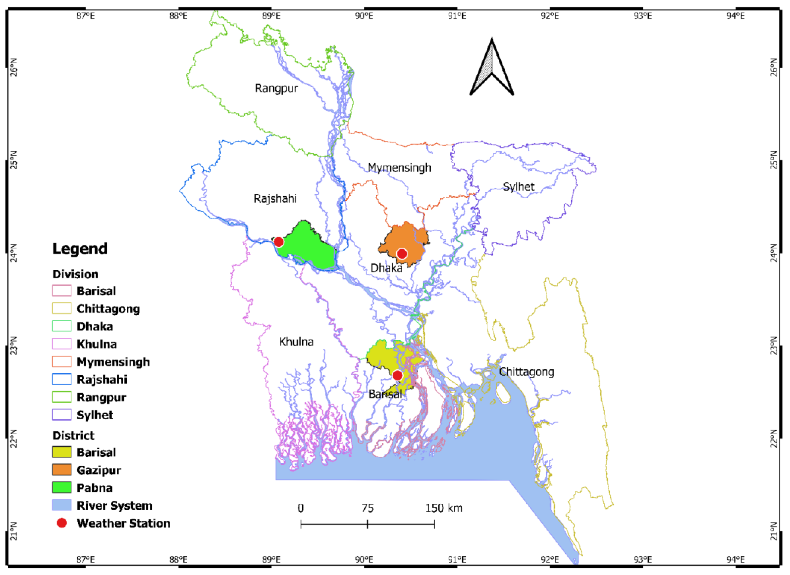
data were collected from three meteorological stations, namely, Barishal, Gazipur, and Ishurdi stations. The selection of these stations was based on their representation of three distinct climatic regions in Bangladesh: (1) Gazipur station represents the central region of Bangladesh, situated at approximately 24.00° N latitude and 90.43° E longitude, with an elevation of 14 m above mean sea level; (2) Ishurdi station represents the northern climatic regions of Bangladesh, located at around 24.04° N latitude and 90.07° E longitude, with an elevation of 18 m above mean sea level; and (3) Barishal station represents the southern part of Bangladesh, positioned at approximately 22.60° N latitude and 90.36° E longitude, with an elevation of 1.0 m above mean sea level. The study area, including the locations of these three weather stations, is depicted in
Figure 1.
This study utilizes medium-term daily temperature data obtained from the Bangladesh Meteorological Department (BMD) across three weather stations to provide multi-step-ahead temperature forecasts. The maximum and minimum temperatures of the day were measured using Zeal P1000 maximum and minimum thermometers from G. H. Zeal Ltd., London, UK. The thermometers have an accuracy of ±0.2 °C and a range and resolution of −50 to +70 °C with 0.1 °C increments, and they were positioned at a measurement height of 2 m. The geographical distribution of meteorological stations is illustrated in
Figure 1, depicting a reasonable coverage of three distinct regions across the country. Notably, Bangladesh’s topography is predominantly flat, with some elevated regions in the northeast and southeast. Consequently, it is reasonable to infer that the selected meteorological stations comprehensively represent the climatic conditions of the three regions of the country [
44].
The temperature distribution in Bangladesh is significantly influenced by various local conditions. The country’s proximity to the equator contributes to a predominantly tropical climate, characterized by high temperatures throughout the year. The Bay of Bengal, bordering the southern coastline, acts as a key influencer, moderating temperatures along the coastal regions compared to the inland areas. The flat topography, interspersed with some upland regions, further contributes to temperature variations. Seasonal monsoons, driven by distinct wind patterns, play a crucial role in shaping temperature dynamics and precipitation patterns, thus exerting a notable impact on the overall temperature distribution across different geographical regions of Bangladesh [
5,
6].
Gazipur station exhibits a tropical wet and dry or savanna climate (classification: Aw). The district records an annual average temperature of 28.95 °C, marking a 1.21% increase compared to the national averages in Bangladesh. Gazipur usually receives around 71.24 mm of precipitation annually. Ishurdi station also features a tropical wet and dry or savanna climate (classification: Aw). The district maintains an annual temperature of 29.52 °C, which is 1.78% higher than the national averages in Bangladesh. Ishurdi typically receives around 98.38 mm of precipitation annually. Barisal station experiences a tropical climate, characterized by significantly less rainfall in winter compared to the summer months. According to Köppen and Geiger [
45], this location falls under the Aw classification. Statistical analysis reveals an average temperature of approximately 25.6 °C, with an annual rainfall of around 2005 mm. The temperate characteristics of Barisal poses challenges in clearly categorizing distinct seasons in the region.
The acquired temperature forecast results remain unaffected by local atmospheric conditions. While the mentioned local factors are implicitly embedded in the data collected from weather stations, it is crucial to note that the modeling outcomes presented in this research solely derive from historical temperature data from BMD.
A diurnal cycle, also known as a diel cycle, manifests as a recurring pattern every 24 h due to the complete rotation of the Earth around its axis. The Earth’s rotation gives rise to temperature variations on the surface during both day and night, contributing to seasonal weather changes. The primary determinant of the diurnal cycle is the influx of solar radiation [
46]. The atmospheric seasonal cycle is influenced by the Earth’s axial tilt. The Earth’s seasonal cycle arises from its 23° axial tilt, causing varying solar radiation at different latitudes throughout the year. Equinoxes align the sun with the equator, the June solstice with the Tropic of Cancer, and the December solstice with the Tropic of Capricorn, creating hemispheric temperature disparities in summer and winter. The Annual Temperature Cycle (ATC) encompasses seasonal temperature changes that are influenced by fluctuations in solar radiation reaching the Earth’s surface throughout the year [
47]. Typically, evaluating the ATC relies on sparse and unevenly distributed air temperature observations or numerical model simulations. This study utilized temperature data collected by the Bangladesh Meteorological Department (BMD) at specific intervals, encompassing daily maximum and minimum values. The data were sourced from three designated weather stations for analysis.
In this study, the daily
and
data were collected from three weather stations, located in distinct climatic regions of Bangladesh. Ensuring the quality of the temperature datasets is essential to enhance the reliability of temperature forecasts using ML algorithms [
48]. While a comprehensive quality assurance process was not conducted for this specific dataset, the accuracy and completeness of the recorded temperature data were systematically assessed using range/limit tests. Range testing is a fundamental quality control method that involves verifying that every observation falls within a specified range [
48]. Only values within the predefined limits are considered valid [
49,
50], while readings outside the specified range are appropriately marked as invalid. The valid readings within the allowable range were used to simulate future temperature fluctuations in the selected weather stations, with a particular focus on generating multi-step forward temperature forecasts for both
and
.
A small portion of the collected data, amounting to less than 2% of the total data from all weather stations, contained missing values. To address this issue, the ‘moving median’ imputation technique was employed. This technique utilizes a moving median with a predetermined window length to fill in the missing values. After applying the imputation method, the weather stations Barishal, Gazipur, and Ishurdi had 2677 readings (from 1 January 2015 to 30 April 2022), 6695 readings (from 1 January 2004 to 30 April 2022), and 2041 readings (from 1 June 2015 to 31 December 2020) of daily and values.
Table 1 presents the descriptive statistics for daily
and
at the three weather stations. It can be seen from
Table 1 that the data exhibited left (negative) skewness, suggesting that the distribution had an extended left tail compared to the right tail. Additionally, kurtosis values included both positive and negative values, indicating that the datasets had both ‘heavy-tailed’ (positive kurtosis) and ‘light-tailed’ (negative kurtosis) distributions.
The Gaussian distribution, commonly known as a normal distribution, is characterized by a bell-shaped curve. It is often assumed that measurements will adhere to a normal distribution, featuring an equal number of measurements above and below the mean. However, in real-world scenarios, data may not precisely conform to the Gaussian distribution and could exhibit slight deviations. In practice, achieving exact conformity to a Gaussian distribution is rare. Ideally, if a distribution is truly normal, the mean, median, and mode values would be identical—an occurrence seldom observed in real-world situations. In instances where the values of the mean, median, and mode differ, the distribution is considered skewed and deviates from the Gaussian norm [
51]. The presented data in
Table 1 reveal that the mean, median, and mode values of the temperature measurements exhibit slight differences. These numerical variations suggest that the data do not perfectly adhere to a Gaussian distribution and show indications of being slightly skewed. The specific numeric values can be found in
Table 1 for reference. Skewness quantifies the asymmetry that is present in data relative to their sample mean. Negative skewness indicates that the data are more dispersed to the left of the mean, while positive skewness suggests greater dispersion to the right. A perfectly symmetric distribution, such as the normal distribution, has a skewness of zero. Kurtosis serves as a metric for gauging the susceptibility of a distribution to outliers. The normal distribution exhibits a kurtosis of 3. Distributions with kurtosis values exceeding 3 are more prone to outliers than the normal distribution, while those with values below 3 are less susceptible. Some definitions of kurtosis involve subtracting 3 from the calculated value, resulting in a kurtosis of 0 for the normal distribution. This study adopts this later definition (subtracting 3 from the calculated value) to compute the kurtosis value.
2.2. Data Preprocessing for the Lagged Input and Output Variables
Time-lagged information was gathered from the collected time series of the daily
and
values. The outputs from the models were the day-ahead
and
values. Therefore, the inputs to the models (five models for five-days-ahead forecasts) were
Due to time-lagging of input variables and the target, the observed daily
and
records were reduced at each weather station. At Barishal station, a total of 2642 historical records remained (from 1 January 2015 to 26 March 2022) after removing 35 records due to time-lagging (5-time lag forward and 30-time lag backward) from the entire time series of 2677 readings (from 1 January 2015 to 30 April 2022). At Gazipur station, a total of 6660 historical records remained (from 1 January 2004 to 26 March 2022) after removing 35 records due to time-lagging (5-time lag forward and 30-time lag backward) from the entire time series of 6695 readings (from 1 January 2004 to 30 April 2022). At Ishurdi station, a total of 2006 historical records remained (from 1 June 2015 to 26 November 2020) after removing 35 records due to time-lagging (5-time lag forward and 30-time lag backward) from the entire time series of 2041 readings (from 1 June 2015 to 31 December 2020). Each station’s remaining dataset was divided into two sets: 80% for model training and 20% for model testing. While there is no established rule for data splitting during model learning and testing [
52], it is recommended that testing data comprise between 10% and 40% of the total dataset size [
53].
2.3. Input Variable Selection
The first step in developing forecast models using ML-based approaches is the selection of the most significant input variables [
39,
40]. For the purpose of choosing input variables in hydrology and water resource modeling [
39], both linear methods [
41] and nonlinear techniques [
40] have been employed. However, because hydrology and water resource modeling issues are frequently nonlinear in nature [
54], linear methods based on Partial Autocorrelation Function (PACF) and Autocorrelation Function (ACF) are often less suitable techniques. For modeling of hydrological and water resources as well as other fields of science and engineering applications, nonlinear approaches that utilize mutual information (MI) [
55] typically outperform linear techniques [
35,
40,
56].
Since the only data used in this effort are the daily
and
values at three weather stations (Barishal, Gazipur, and Ishurdi), the time-lagged versions of the acquired temperature data (from each station) were used as potential inputs. To extract the time-lagged information from the
and
time series and choose which lags to include as prospective inputs, the PACF was employed. The PACF is a technique that is commonly used in time series analysis to identify the most influential lagged features for predicting a target variable [
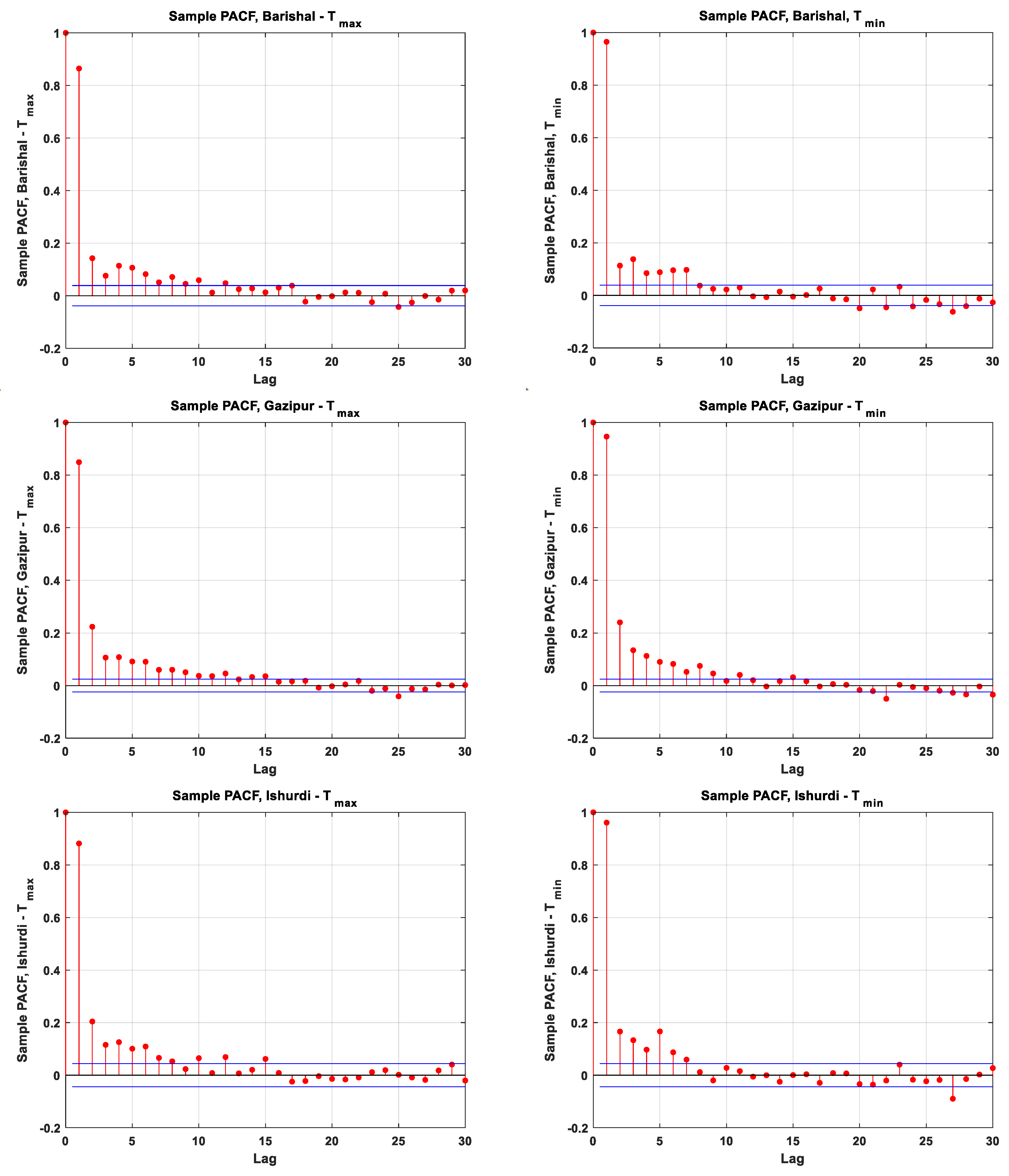
57]. The PACF measures the correlation between a time series variable and its lagged values, while accounting for the influence of intermediate lags. By applying PACF, one can identify the lagged features that have the most significant impact on the target variable. These lagged features capture the historical patterns and dependencies that can be exploited for accurate time series forecasting.
Figure 2 displays the PACF plots for the data from three weather stations, revealing that the current and past 30-time lags are essential for forecasting temperatures for the next five days (
). The PACF provided an initial guess of the candidates for input variables. However, this initial selection of input variables may include unnecessary or redundant features, which could hinder the training of ML-based forecasting models. Therefore, it is important to determine the most significant input variables to ensure proper training and computational efficiency.
Next, this study used the F-statistic [
58,
59] to identify the most influential input variables. The F-test is a statistical test that assesses how much the variability in the target variable is explained by a specific feature compared to the variability that is not explained by that feature. It examines the importance of each predictor individually using an F-test, testing the hypothesis that the response values that are grouped by predictor variable values are drawn from populations with the same mean against the alternative hypothesis that the population means are not all the same. A small
p-value of the F-test indicates the importance of the corresponding predictor. The F-statistic is calculated by dividing the mean square regression (MSR), representing explained variability, by the mean square error (MSE), representing unexplained variability. Univariate feature ranking with F-tests helps identify the most influential features for a regression task, emphasizing the most relevant variables and potentially enhancing interpretability and model performance [
58,
59].
The variable importance is also determined using the MRMR technique [
60,
61]. The MRMR algorithm aims to find a balance between selecting informative features while avoiding redundant ones. MRMR considers both relevance and redundancy when identifying a subset of features that collectively offer maximum information while minimizing duplication. There are variations and extensions of MRMR, such as weighted MRMR or incremental MRMR, which provide additional flexibility and adaptability to different scenarios. Overall, MRMR is a valuable feature selection technique that enhances the interpretability, generalization, and efficiency of machine learning models by focusing on the most relevant and nonredundant features. The MRMR algorithm [
61] identifies a best-possible set of characteristics that are maximally and mutually different and are useful for representing the response variable. The approach maximizes a feature set’s relevance to the response variable while minimizing its redundancy. Using pairwise mutual information of attributes and mutual information of an attribute and the response, the technique measures the degree of duplication as well as the relevance of variables.
The MRMR technique seeks to identify an ideal set
of features that maximizes
, the relevance of
pertaining to a response variable
, and minimizes
, the redundancy of
, where
and
are defined with mutual information (MI)
:
where
denotes the quantity of attributes in
. The amount of uncertainty in one variable that can be lowered by understanding the other variable is measured by the MI between two variables.
The MI
of the discrete random variables
and
can be represented by [
60]
If and are independent, then equals 0. If and are the same random variable, then equals the entropy of .
It is necessary to take into account all
combinations in order to find the optimum set
, where
is the set of all features. The MRMR approach utilizes an alternative approach. In this approach, the MRMR approach scores attributes by employing the forward addition technique, which necessitates
computations, by utilizing the MI quotient (
MIQ) value.
where
and
are the relevance and redundancy of a feature, respectively:
The MRMR function uses a heuristic technique to quantify the significance of a characteristic and then generates a score. A high score value denotes the significance of the associated predictor. A degree of trust in feature selection is also indicated by a decline in the feature significance score. The score value of the second most essential attribute, for instance, is significantly lower than the score value of if the algorithm is confident in choosing it. The results can be used to identify an ideal set for a particular collection of features.
The features were ranked using the MRMR algorithm according to the following steps:
Step 1: Select the feature with the largest relevance, . Add the selected feature to an empty set .
Step 2: Find the features with nonzero relevance and zero redundancy in the complement of , .
If does not include a feature with nonzero relevance and zero redundancy, go to step 4.
Otherwise, select the feature with the largest relevance, . Add the selected feature to the set .
Step 3: Repeat Step 2 until the redundancy is not zero for all features in .
Step 4: Select the feature that has the largest
MIQ value with nonzero relevance and nonzero redundancy in
, and add the selected feature to the set
.
Step 5: Repeat Step 4 until the relevance is zero for all features in .
Step 6: Add the features with zero relevance to in random order.
Feature selection using Neighborhood Component Analysis (NCA) [
62] focuses on learning a transformation matrix that preserves the discriminative information in the data while reducing the dimensionality. By considering the local neighborhood relationships between data points, NCA can identify the most informative features for the task at hand. It is important to note that NCA assumes linearity in the data and may not capture complex nonlinear relationships. Therefore, it is advisable to combine NCA with nonlinear dimensionality reduction techniques or explore other feature selection methods for capturing nonlinear feature interactions if needed. The NCA feature selection for regression can be mathematically represented as follows [
62]:
Given observations where the response values are continuous, the aim is to predict the response given the training set .
Consider a randomized regression model that:
Again, the probability
that point
is picked from
as the reference point for
is
Now consider the leave-one-out application of this randomized regression model, that is, predicting the response for
using the data in
and the training set
excluding the point
. The probability that point
is picked as the reference point for
is
Let
be the response value that the randomized regression model predicts and
be the actual response for
. And let
be a loss function that measures the disagreement between
and
. Then, the average value of
is
After adding the regularization term, the objective function for minimization is
The default loss function for NCA for regression is mean absolute deviation.
In this study, a combination of variable selection methods (F-tests, MRMR, and NCA) was used to select the most significant input variables from an initial pool of 30 candidate inputs determined by PACF. To include all possible contributing variables affecting the outputs, all variables selected by the individual variable selection approaches were considered, while the common variables determined by all approaches were used only once. Doing so eliminates the possibility of excluding any variables which might have been deemed important to forecast the output. Using this combinatory variable selection scheme, the possible number of candidate variables of the inputs for one-, two-, three-, four-, and five-days-ahead forecast of at Barishal station were 26, 27, 26, 22, and 25, respectively. The number of candidate variables of the inputs for one-, two-, three-, four-, and five-days-ahead forecast of at Barishal station were 21, 22, 24, 24, and 23, respectively. Similarly, the possible number of candidate input variables for one-, two-, three-, four-, and five-days-ahead forecast of at Gazipur station were 25, 26, 25, 24, and 25, respectively. The number of candidate input variables for one-, two-, three-, four-, and five-days-ahead forecast of at Gazipur station were 26, 25, 26, 25, and 25, respectively. Likewise, the possible number of candidate variables of the inputs for one-, two-, three-, four-, and five-days-ahead forecast of at Ishurdi station were 23, 23, 26, 26, and 26, respectively. The number of candidate variables of the inputs for one-, two-, three-, four-, and five-days-ahead forecast of at Ishurdi station were 24, 28, 21, 23, and 21, respectively.
2.4. Model Development
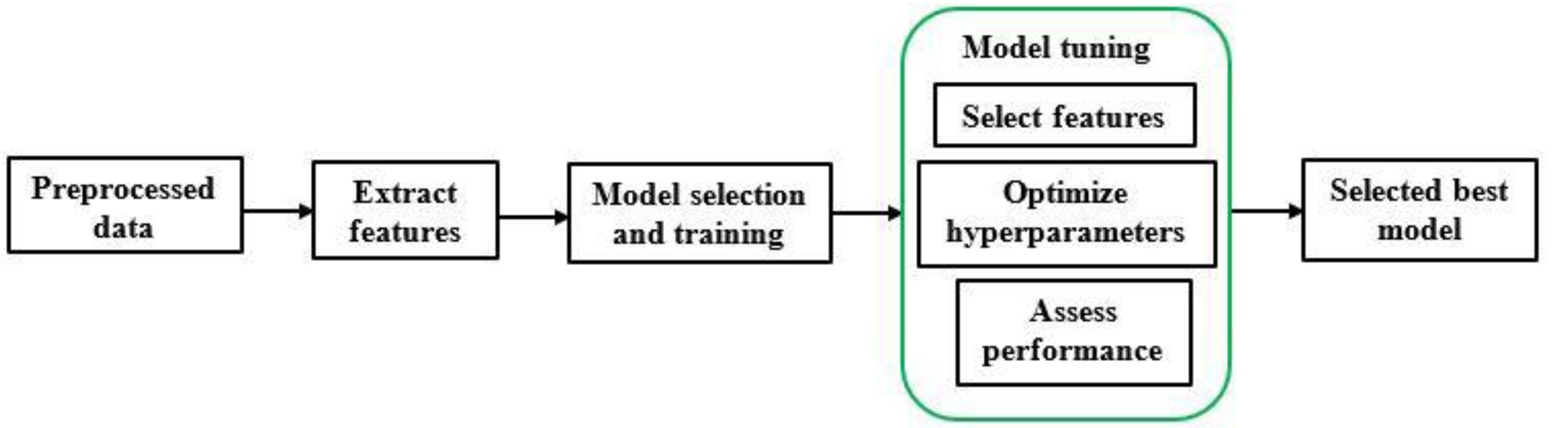
The accuracy and robustness of any forecasting model largely depend on the right selection of models and their forecasting accuracy. Forecasting models are developed using training and testing of the state-of-the-art machine learning algorithms, the optimal parameters of which were decided here based on parameters tuning using the Bayesian and ASHA optimization algorithms. Training several models and finding their optimal parameter sets through hyperparameter tuning can often be a challenging and time-consuming task. This task was made easier and faster by developing and comparing multiple models automatically through tuning their hyperparameters using optimization algorithms. In this approach, instead of training each model with different sets of hyperparameters, we selected a few different models and tuned their default hyperparameters using Bayesian and ASHA optimizations. These optimization algorithms search for an optimal set of hyperparameters for a particular model by minimizing the objective function of the model (minimization of the mean squared error (MSE)). The optimization algorithms deliberately selected new hyperparameters in each iteration, produced an optimal set of hyperparameters for a given training dataset, and identified the model that performed best on a test dataset. With the Bayesian and ASHA optimization algorithms, the function randomly selected several models with various hyperparameter values and trained them on a small subset of the training data. If the log (1 + valLoss) value for a particular model was found promising, where valLoss is the cross-validation MSE, the model was promoted and trained on a larger amount of the training data. This process was repeated, and successful models were trained on progressively larger amounts of data. To reiterate, our proposed approach executed the following three steps simultaneously in the model development process:
Data exploration and preprocessing: Identify variables with low predictive power that should be eliminated.
Feature extraction and selection: Extract features automatically and—among a large feature set—identify those with high predictive power.
Model selection and tuning: Automatically tune model hyperparameters and identify the best-performing model.
The flow diagram of the entire model building process can be illustrated as
Figure 3.
2.5. Hyperparameter Optimization
The majority of ML algorithms require a careful selection of hyperparameters [
63]. The choice of hyperparameter settings significantly impacts the performance of ML models [
64], and unconscious hyperparameter selection can result in low-performing models. Many studies employed trial-and-error selection of hyperparameters [
64,
65], grid search, and/or random search [
66], while some employed heuristic optimization algorithms like particle swarm optimization and genetic algorithms [
66]. Nevertheless, a precise and effective automated hyperparameter optimization method is highly desirable [
64] and is essential for ensuring a fair comparison across ML alternatives. Furthermore, when evaluating various ML models, fair assessments can only be made if they are equally optimized (or receive the same level of attention) for the specific task at hand.
Bayesian optimization and asynchronous successive halving algorithm (ASHA) are advanced optimization techniques that are employed to automate and enhance the efficiency of model selection processes. In Bayesian optimization, a probabilistic model is iteratively updated to capture the relationship between model hyperparameters and performance, guiding the search toward promising regions of the parameter space. This process allows for intelligent and resource-efficient exploration, especially in scenarios with limited computational resources. On the other hand, ASHA introduces an asynchronous approach to hyperparameter optimization, enabling parallel evaluations and efficient resource utilization. By continually pruning underperforming models, ASHA converges to optimal hyperparameter configurations. ASHA is particularly beneficial in scenarios with limited computational resources or asynchronous evaluations. It employs a successive halving strategy to efficiently allocate resources to promising configurations, eliminating less favorable ones. Both Bayesian optimization and ASHA contribute significantly to automating the selection of suitable models, particularly in the context of temperature forecasting, where manual selection can be time-consuming and subjective. The combination of these algorithms in this study represents a novel and valuable contribution to the field, showcasing their effectiveness in optimizing hyperparameters and improving the overall accuracy of temperature prediction models.
A state-of-the-art approach for both global and local hyperparameter optimization is known as Bayesian optimization (BO) [
37]. BO has been shown to outperform alternative methods like grid search and random search on various challenging optimization benchmarks [
66]. In the quest for discovering the best hyperparameters, BO often surpasses the abilities of domain experts [
67]. BO is versatile and applicable to a wide range of problem scenarios, accommodating both integer and real-valued hyperparameters. BO relies on the selection of a prior function and an acquisition function. The acquisition function, typically employing Expected Improvement (EI), works in conjunction with a Gaussian process prior [
37]. The choice of covariance function, particularly the use of the Matern52 kernel, is crucial In determining the effectiveness of Gaussian processes [
37]. With respect to
in a bounded domain, the BO algorithm process seeks to minimize a scalar objective function,
. Depending on whether the function is stochastic or deterministic, it may yield different results when evaluated at the same point
. The variable
can have continuous real values, integers, or categorical components, referring to a discrete set of names. The key components in the minimization process include [
68]:
A Gaussian process model of ).
A Bayesian update procedure for modifying the Gaussian process model at each new evaluation of .
An acquisition function (based on the Gaussian process model of ) that is maximized to determine the next point for evaluation.
The ASHA [
38] optimization algorithm is an upgraded variant of the successive halving algorithm (SHA) [
69,
70]. ASHA is a user-friendly hyperparameter optimization technique that leverages aggressive early stopping and is particularly suited for tackling large-scale hyperparameter optimization problems [
38]. It has demonstrated superior performance on a workload employing 500 workers, exhibits linear scalability with the number of workers in distributed environments, and is well-suited for tasks involving substantial parallelism [
38]. An advantage of ASHA is that the user does not need to specify in advance how many configurations they want to evaluate, because it operates asynchronously. However, it still requires the same inputs as SHA. A comprehensive explanation of ASHA can be found in the original work by Li et al. [
38] and is not repeated in this effort.
To the best of the authors’ knowledge, this is the first instance of the Bayesian and ASHA optimization algorithms being employed to tune the hyperparameters of multiple ML algorithms to automatically select the best model for forecasting multi-step-ahead daily
and
. In this study, forecasting models were developed by fine-tuning hyperparameters of seven widely utilized ML algorithms, aiming to identify the optimal model for forecasting daily
and
.
Table 2 outlines the candidate ML algorithms and their adjustable hyperparameters. The hyperparameters were tuned using both the Bayesian and ASHA optimization algorithms, and a comparison was performed with respect to training time and accuracy. The best model was selected based on its ability to yield the lowest training and test errors, employing either the Bayesian or ASHA optimization algorithms.
Forecasting models were developed for one-, two-, three-, four-, and five-days-ahead forecasting of daily and using data from three weather stations. Consequently, a total of 30 forecasting models were chosen by applying Bayesian and ASHA optimization techniques. Each training dataset, consisting of input–output pairs, was divided into a training set, containing 80% of the data, and a test set, containing the remaining 20%. To enhance computational efficiency, both algorithm runs were executed in the parallel computing environment of MATLAB (MATLAB, 2021a).
2.6. Statistical Indices for Performance Evaluation
The following statistical indices were used to evaluate the performances of the developed temperature forecast models. The accuracy index is an evaluation metric that compares the proportion of accurate forecasts made by a model to all forecasts made. The higher the accuracy score is, the better the model performance will be. The ideal value of accuracy is 1.0. The correlation coefficient, R, denotes the strength of linear regression between the observed and forecasted values; however, for this linear relationship, the highest possible value (ideal) of R = 1.0 can be obtained despite the fact that the slope and ordinate intercept are different from 1.0 and 0, respectively [
53]. Therefore, other indices need to be used to justify the model performance. A normalized/dimensionless measure of residual variance, Nash–Sutcliffe Efficiency Coefficient (NS) metric, is calculated by dividing residual variance by variance of observed dataset. NS ≤ 0.4, 0.40 < NS ≤ 0.50, 0.50 < NS ≤ 0.65, 0.65 < NS ≤ 0.75, and 0.75 < NS ≤ 1.00 are categories that are labeled as unsatisfactory, acceptable, satisfactory, good, and exceptionally good, respectively [
71,
72]. Willmott’s Index of Agreement (IOA) [
73] is able to detect additive and proportional differences in the observed and model-forecasted means and variances. The IOA usually ranges from −1 to +1, with higher values indicating greater model performance. Nevertheless, the IOA is often overly sensitive to extreme values due to the squared differences [
74]. The Kling Gupta Efficiency (KGE) [
75,
76], which combines the three components of model errors (i.e., correlation, bias, and ratio of variances or coefficients of variation) in a more balanced way, has been widely used for evaluating the prediction ability of models in recent years.
Generally, the RMSE criterion measures the error of the model. A lower value of RMSE indicates a higher forecasting power of the model. However, the value of RMSE largely depends on the magnitude of the data, and therefore, a lower value of RMSE does not necessarily mean a better forecasting performance. To overcome this issue, the NRMSE criterion was used to eliminate the dimensionality effect of the data. Model performance is said to be excellent when NRMSE is less than 0.1, good when NRMSE is between 0.1 and 0.2, fair when NRMSE is between 0.2 and 0.3, and poor when NRMSE is greater than 0.3 [
77,
78]. The Mean Absolute Percentage Relative Error (MAPRE) is the most common measure used to evaluate a model’s prediction performance, probably because the variable’s units are scaled to percentage units, which makes it easier to understand. It works best if there are no extremes to the data (and no zeros). It is often used as a loss function in regression analysis and model evaluation. Median Absolute Deviation (MAD) is a resistant measure of variability, as it relies on the median as the estimate of the center of the distribution and on the absolute difference rather than the squared difference. Because the MAD is the median deviation of scores from the overall median, not all observations are equally weighted in this measure of dispersion. The clear advantage of MAD is the avoidance of influence by outliers. However, it has its own problems: if the distribution is actually normal, there is a loss of efficiency, in that it does not make as much use of the information as what is available in the data [
79]. The MBE criterion provides an estimation of whether the developed model systematically under- or over-predicts the actual values. The MBE is usually not used as a measure of the model error, as high individual errors in prediction can also produce a low MBE. MBE is primarily used to estimate the average bias in the model and to decide if any steps need to be taken to correct the model bias [
80]. The Percentage Bias (PBIAS) measures the average tendency of the simulated values to be larger or smaller than their observed ones. The optimal value of PBIAS is 0.0, with low-magnitude values indicating accurate model simulation. Positive values indicate overestimation bias, whereas negative values indicate model underestimation bias.
Correlation coefficient (R) [
82]:
Nash–Sutcliffe Efficiency Coefficient (NS) [
83]:
Willmott’s Index of Agreement (IOA) [
73]:
Kling–Gupta Efficiency (KGE) [
75,
76]:
Root mean squared error (RMSE) [
74]:
Mean Absolute Percentage Relative Error (MAPRE) (MAPE, n.d.):
Median Absolute Deviation (MAD) [
85]:
Mean Bias Error (MBE) [
86]:
Percentage Bias (PBIAS) [
87,
88]:
where
and
are the observed and forecasted
(
) for the
data point in the daily maximum and minimum temperature dataset, respectively;
and
are the means of the observed and forecasted
(
), respectively; and
represents the total number of entries in the dataset.
3. Results and Discussion
A range of statistical performance evaluation indices, as discussed in the previous section, were employed to assess the performance of the various forecasting models. In the subsequent paragraphs, the performances of the identified top-performing models on the test dataset (selected based on their performance on both the training and test datasets) for the five forecasting horizons at the three stations are presented.
Table 3 provides a comparison of the best models that were selected by the Bayesian and ASHA optimization algorithms, considering log(1 + valLoss) values and training time for multi-step-ahead
forecasting. As can be observed from the log(1 + valLoss) value presented in
Table 3, the Bayesian optimization algorithm generally outperformed the ASHA algorithm in selecting the best model. However, in terms of training time, the ASHA algorithm demonstrated faster convergence in finding the optimal model parameters compared to the Bayesian algorithm. However, while the ASHA algorithm showed competitive performance in terms of training time, the Bayesian algorithm also achieved convergence within acceptable time limits. Therefore, in cases where training time is not a critical factor, the Bayesian optimization can be used to find optimal model parameters for selecting the best models for a specific task. On the other hand, when training time is a more important consideration than model accuracy, the ASHA optimization algorithm is advisable. Notably, there were instances where the ASHA algorithm outperformed the Bayesian algorithm in both log(1 + valLoss) and training time, such as for the one-step-ahead
forecast at Barishal station and four-step-ahead
forecast at Ishurdi station. In cases where the Bayesian algorithm showed superior performance based on log(1 + valLoss) values, the differences were not substantial, while there was a significant difference in training times between the two algorithms.
Table 4 presents the training and test performance results of the Bayesian and ASHA algorithm-tuned forecast models for maximum temperatures (
) at the weather stations. At this stage, the final models were selected based on the RMSE criterion: the best models were those producing the lowest difference between the training and test RMSE values. This ensures that the selected best models were neither over-trained nor under-trained. The data in
Table 4 reveal that the ASHA algorithm-tuned best models produced the lowest difference between the training and test RMSE values in most instances (forecasting horizons and weather stations) for forecasting
values. Although the Bayesian algorithm required a longer time to converge to optimal solutions for selecting the best models, it excelled in three specific instances: the one-day- and five-days-ahead
forecast at Barishal station, and the three-days-ahead
forecast at Gazipur station (as indicated in
Table 4). A complete list of the selected top-performing models can be found in Table 7.
Table 5 provides a comparative performance evaluation of the Bayesian and ASHA algorithm-tuned best models for forecasting
at the weather stations, based on log (1 + valLoss) values and training time requirements.
The results in
Table 5 reveal that, in terms of log (1 + valLoss) values, the Bayesian algorithm-tuned best models outperformed the ASHA algorithm-tuned models in all instances except for the two-days-ahead forecast at the Gazipur station, where the ASHA algorithm-tuned GPR model was found to be the top-performing best model. Moreover, the ASHA algorithm-tuned models exhibited faster convergence to optimal solutions for parameter values in comparison to the Bayesian algorithm-tuned models in all instances. Additionally, the differences between the training errors (log (1 + valLoss)) produced by the Bayesian and ASHA algorithms for selecting the best models were relatively small for all instances. In summary, when computational time is not a limiting factor, the Bayesian algorithm is a suitable choice for searching for the best models (
Table 5). However, it is essential to carefully evaluate the differences between the training and test errors of the best models that are produced by the Bayesian and ASHA algorithms before making a definitive decision on model selection.
The comparison of the training and testing performance between the Bayesian and ASHA optimization-tuned best models for forecasting
at the weather stations, as assessed by the RMSE criterion, is presented in
Table 6. It is evident from
Table 6 that both the Bayesian and ASHA algorithms exhibited similar performance in selecting the top-performing best models across all forecasting horizons and at all weather stations. The Bayesian algorithm outperformed in seven instances, while the ASHA algorithm provided top-performing forecast models in eight instances based on the lowest differences between the training and test RMSE values (
Table 6). Overall, the selected top-performing best models demonstrated acceptable results according to the RMSE criterion. However, further validation of the forecasting performance of the selected models is required by computing other performance evaluation indices on the test dataset. A comprehensive performance evaluation of the selected top-performing models based on several statistical indices can be found in Table 8 and Table 9 and
Figure 3 and
Figure 4.
The complete list of the selected best models for different weather stations under five forecasting horizons, based on log (1 + valLoss), RMSE, training time, and differences between the training and test RMSE (as presented in
Table 3,
Table 4,
Table 5 and
Table 6), is provided in
Table 7.
Following the selection of the best-performing models, they were utilized to forecast multi-step-ahead
and
values on the test dataset at the respective weather stations. To evaluate the forecasting performance, various statistical performance indices were computed and are presented in
Table 8 and
Table 9. Additionally, the results are visualized in
Figure 3 and
Figure 4.
Table 8 presents a comprehensive overview of the performance of the best models in forecasting
under five different forecast horizons at the weather stations. It can be observed from
Table 8 that the selected models consistently produced lower values of various performance metrics such as RMSE, NRMSE, MAPRE, MAD, MBE, and PBIAS. This indicates that the models have demonstrated improved accuracy in forecasting
. It is also inferred from the results presented in
Table 8 that the forecasting performance slightly decreased with an increase in the forecast horizon. This observation aligns with prior findings reported in studies by Rahman et al. [
42] and Barzegar et al. [
89], which indicated that ML-based forecast models tend to exhibit reduced accuracy as the forecast horizon extends further into the future. The RMSE values were pretty small for all selected models across the weather stations. Small RMSE values generally indicate that the models’ predictions are closely aligned with the actual observations, suggesting a high level of accuracy in the forecasts. The NRMSE values were consistently less than 0.1 for all instances. An NRMSE below 0.1 is considered excellent performance in forecasting, as it indicates that the forecasted values are very close to the actual values [
77,
78]. The MAPRE values are also within acceptable ranges. For Barishal, Gzipur, and Ishurdi stations, the MAPRE values were below 8% (ranging from 5.091% to 7.954% for different forecast horizons), 7% (ranging from 4.737% to 6.468% for different forecast horizons), and 6% (ranging from 4.728% to 5.426% for different forecast horizons), respectively, depending on the forecast horizons. Since a MAPRE value below 10% is deemed acceptable for ML-based forecast models [
90], these results suggest that the selected models are producing forecasts that meet or exceed acceptable standards. In summary, these performance indices demonstrate that the selected best forecast models are capable of producing accurate and reliable forecasts for
values at the weather stations, as evidenced by their small RMSE and NRMSE values, as well as MAPRE values that are well within the acceptable range.
The MAD values are also reported as being acceptable for all models. These values ranged from 0.634 °C for a one-day-ahead forecast at Gazipur station to 1.070 °C for a five-days-ahead forecast at Barishal station. The lower the MAD is, the closer the forecasts are to the actual values, indicating accurate model forecasts. Additionally, the models produced smaller values of MBE and PBIAS, which were pretty close to the optimal value of 0.0. MBE quantifies the average bias (overestimation or underestimation) in the forecasts, while PBIAS provides a measure of the Percentage Bias. The models produced low-magnitude values of both MBE and PBIAS, indicating that they are making reasonably accurate forecasts. Some models show negative MBE and PBIAS values, indicating a slight underestimation bias, particularly for Gazipur and Ishurdi stations and for three-days-ahead forecasts at Barishal station. On the other hand, positive MBE and PBIAS values are observed for one-day-, two-days-, four-days-, and five-days-ahead
forecasts at the Barishal station, suggesting a slight overestimation bias (
Table 8). These biases are of smaller magnitude, indicating that the models tend to slightly under-predict or over-predict temperature values, but the deviations from the actual values are not substantial. In summary, the forecast models are delivering forecasts with acceptable levels of accuracy, as indicated by the MAD, MBE, and PBIAS values. While some models exhibit slight underestimation or overestimation biases, these biases are relatively small, and the forecasts are still considered accurate. These results provide confidence in the performance of the selected forecast models.
Table 9 presents a comprehensive assessment of the performance of the top-performing models for forecasting
values under the five forecast horizons at the weather stations. It can be seen from
Table 9 that the overall forecasting performances of the models are acceptable, although the models showed slightly poor performance with respect to the computed RMSE, NRMSE, and MAPRE values when compared to the forecasting of
(
Table 8). Nevertheless, the models produced lower RMSE values (
Table 9). The computed NRMSE criterion suggests that the model performances were excellent (NRMSE < 0.1) to good (NRMSE values slightly higher than 0.1, i.e., NRMSE > 0.1 and NRMSE < 0.2) according to the ranges reported in Heinemann et al. [
77] and Li et al. [
78]. On the other hand, the models produced lower MAD, MBE, and PBIS values compared to those for the models developed for forecasting
(
Table 8 and
Table 9). It is noted that the computed MBE and PBIAS values were pretty close to the ideal value of 0.0. According to the MBE criterion, the models produced very small amounts of underestimated biases, as indicated by the negative MBE values for all forecasting horizons and at all weather stations (
Table 9). Similarly, the PBIAS criterion also suggests that mostly underestimated biases existed, except for the model developed to forecast
for two-step-ahead at the Barishal weather station.
The findings are reported in the form of bar diagrams, especially to demonstrate the model performance based on some other statistical performance indices.
Figure 4 and
Figure 5 illustrate the models’ performance with respect to accuracy, R, NS, IOA, and KGE criteria. These performance indices are referred to as benefit indices, because higher values of these indices indicate improved model performance.
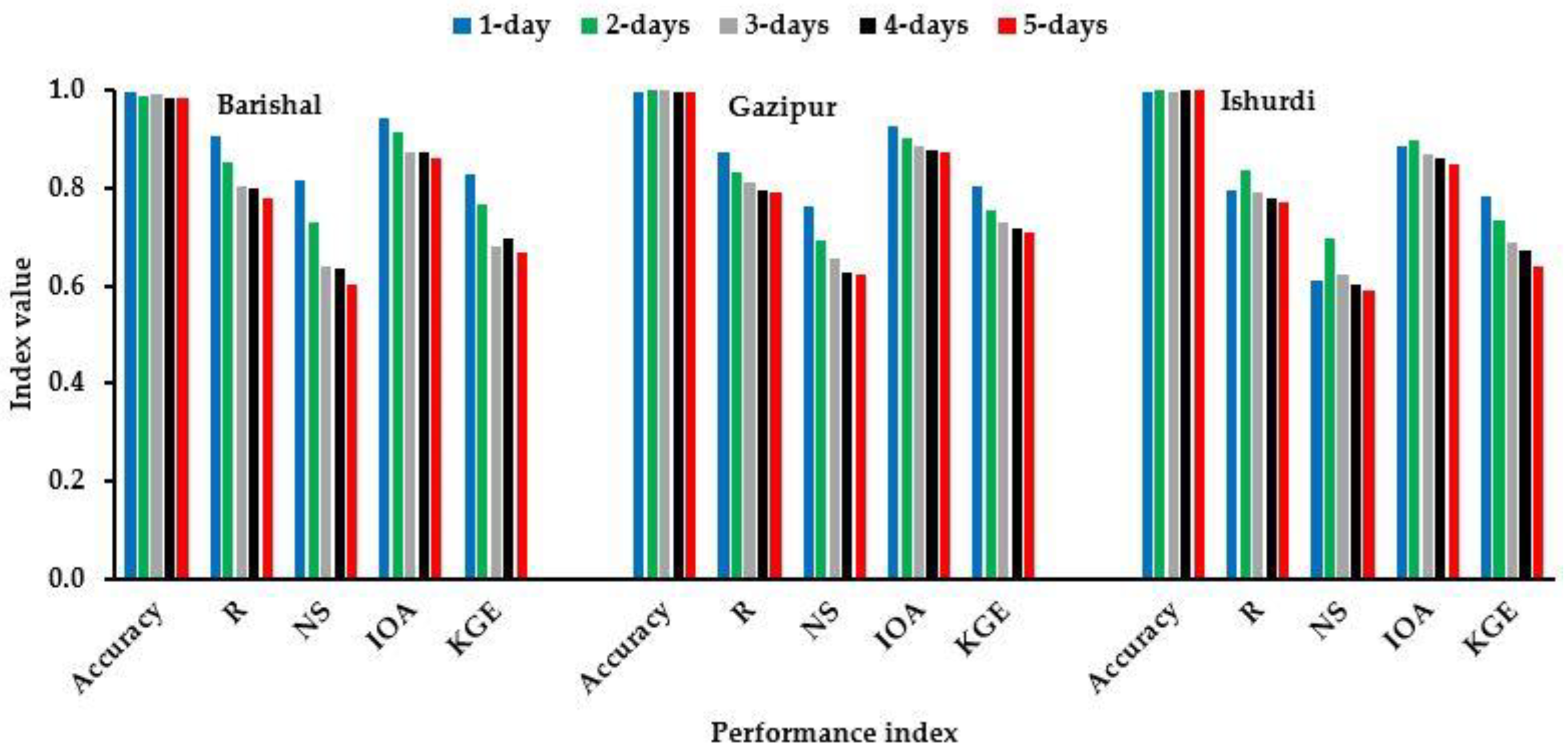
Figure 4 shows the performance of the best models on the test dataset when forecasting
across different forecast horizons at the respective weather stations. This visual representation allows for a quick and easy assessment of how well the models are performing and how their performance varies with different lead times (forecast horizons).
Figure 4 reveals important insights into the performance of the best models for forecasting
under different forecast horizons at the weather stations. It is perceived from
Figure 4 that the best models consistently demonstrate excellent performance with regard to the accuracy and IOA criteria, where accuracy values are close to 1, and IOA values exceed 0.8 for all forecast horizons. This indicates that the models produce forecasts that closely align with observed data and show a strong agreement with the reference measurements. Notably, the accuracy criterion does not exhibit a decreasing trend with an increase in the forecast horizon. In other words, the models maintain high accuracy regardless of the lead time. This is a positive finding, suggesting that the models are reliable for both short-term and longer-term forecasts. However, the R, NS, IOA, and KGE values indicate that the model performance is indeed influenced by the forecast horizon. These indices suggest that the forecasting performance tends to decrease as the forecast horizon increases, which is consistent with prior research [
42,
89]. R values are higher than 0.8 for the first and second forecast horizons (one- and two-step-ahead forecasts) at all weather stations. However, a decrease in R values is observed as the forecast horizon extends, with the lowest R value (0.771) occurring at the fifth forecast horizon for the Ishurdi station. In general, model performances were relatively poor with respect to the NS and KGE criteria (
Figure 4). The findings of this research is in good agreement with the findings presented in Müller and Piché [
91], who stated that ML-based models often showed contrasting performance with respect to different performance evaluation indices. These findings collectively suggest that the models are especially well suited for shorter-term forecasts, but they still provide valuable forecasts for longer lead times, albeit with slightly reduced performance.
In order to forecast
at the weather stations over a range of forecast horizons, the best models were tested against the test dataset. The findings are presented in
Figure 5, which shows the performance of the best models for forecasting
under various forecast horizons at the weather stations.
Figure 5 suggests that the selected top models performed exceptionally well for all forecast horizons and at all the weather stations. This is particularly evident from the accuracy and IOA values, which consistently exceed 0.95. Such high accuracy and IOA values indicate excellent model performance, suggesting that the models generate forecasts that closely match the observed data. Similar to the
forecast, the accuracy of the models remains high across different forecast horizons, with accuracy values close to 1. This indicates that the models maintain their high forecasting accuracy regardless of the lead time. Contrary to accuracy, other performance evaluation indices, including NS, IOA, and KGE, display a diminishing trend as the prediction horizon is extended. This is in line with the common observation that the forecasting performance tends to decrease as the forecast horizon increases, which aligns with the results observed for
forecasting. It is important to note that the R values appear to be consistent across all weather stations. These values are high, exceeding 0.90, indicating a strong correlation between the model forecasts and the observed data. In general, the best models appeared to perform better across all forecast horizons based on the R (>0.90), NS (>0.81), and KGE (>0.87) criterion values. Overall, the findings from
Figure 5 suggest that the selected models perform remarkably well in forecasting
over various forecast horizons and at different weather stations. The models exhibit high accuracy, strong correlations, and consistent performance across forecast horizons, even though other indices show a slight decrease with an increasing forecast lead time.
In a comparative context, the results for forecasting seem to outperform those for forecasting. This improvement in forecasting performance might be attributed to the quality and volume of the collected data. High-quality and abundant data often lead to more accurate forecasts.
While direct comparisons among the results presented in this research are hindered by the diverse study conditions and modeling approaches employed, an indirect evaluation was conducted by contrasting the computed performance indices in this study with those in previous research. For one-day-ahead minimum temperature forecasts, R
2 values of 0.939, 0.911, and 0.901 were achieved across the Barishal, Gazipur, and Ishurdi stations, respectively. Conversely, for one-day-ahead maximum temperature forecasts, R
2 values of 0.819, 0.764, and 0.633 were obtained for the same stations. These results surpass the outcomes of previous studies utilizing CNN (~0.5), LSTM (~0.6), and CNN-LSTM (~0.7) for one-day-ahead temperature forecasts [
33].
Moreover, our findings compare favorably or even outperform those of Ebtehaz et al. [
27], who utilized IORELM for 10 h ahead temperature forecasts (R = 0.95, NSE = 0.89, RMSE = 3.74, MAE = 1.92). Our best models yielded RMSE values of approximately 2.0 °C and 1.5 °C for one-day-ahead maximum and minimum temperature forecasts, respectively. The detailed statistical performance indices for the proposed best models are provided in
Figure 4 and
Figure 5, as well as in
Table 8 and
Table 9.
Furthermore, our research outcomes stand up well against those of Fister et al. [
29], focusing on the temperature dataset of the Paris region. Our proposed best model exhibited superior performance compared to Lasso Regression, Decision Tree, Adaboost, RF, and CNN in terms of MSE values. Alomar et al. [
17] identified the SVR model as the top performer for daily temperature forecasting, achieving an RMSE value of 3.592 °C, which is higher than the RMSE values produced by our proposed best models for both minimum and maximum temperature forecasts across the three weather stations (refer to
Table 8 and
Table 9).
In terms of the RMSE criterion, our proposed best models demonstrated comparable or superior performance (RMSE ~ 2 °C for both minimum and maximum temperatures) compared to the ANN (RMSE ~ 3 °C), GEP (RMSE ~ 3 °C), and HBA-ANN (RMSE ~ 2 °C) models that were developed for the coldest and warmest regions globally [
23]. Based on this comprehensive comparison, it can be argued that our proposed best models exhibit acceptable and sometimes superior performance compared to recently proposed machine and deep learning models for temperature forecasting. However, it is important to note that direct comparisons are challenging due to variations in data and study locations.
The research on automated model selection using Bayesian optimization and the asynchronous successive halving algorithm for predicting daily minimum and maximum temperatures holds crucial implications for the agricultural domain. Accurate temperature predictions are fundamental to agricultural planning, impacting crop growth, yield estimation, and resource allocation. The application of Bayesian optimization ensures a thorough exploration of model parameters, enhancing the precision of temperature forecasts, which is crucial for optimal crop management. The incorporation of the asynchronous successive halving algorithm contributes to computational efficiency in finding the optimal hyperparameters for the selected best models. As a result, this research has the potential to significantly improve agricultural productivity, resource utilization, and resilience to climate variability, ultimately benefiting farmers and stakeholders across the agricultural supply chain.
4. Conclusions
Accurate and reliable forecasting of daily maximum () and minimum () temperatures can be effectively utilized in the development of a sustainable and efficient agricultural water management strategy. However, due to nonlinear interactions between temperatures and other explanatory variables, as well as their multi-scale behavior that changes over time, producing reliable temperature () forecasts is often challenging. The prerequisites for creating accurate ML-based forecast models include selecting only the most influential input variables from a list of prospective input variables and optimizing model parameters. To address these challenges, this study proposes an innovative approach for selecting the most influential input variables and determining the best predictive models for forecasting daily and values. These methods were combined with Bayesian and ASHA hyperparameter tuning to perform automated model parameter estimation. Notably, this study is the first to utilize the Bayesian and ASHA algorithms for automating the model selection process to provide accurate and forecasts at different weather stations in Bangladesh. Furthermore, the study provides a comparison of the best models that are tuned with Bayesian and ASHA algorithms. The selected best models were explored for one-, two-, three-, four-, and five-days-ahead and forecasting. The top-performing models for different forecasting horizons (1-day-, 2-days-, 3-days-, 4-days-, and 5-days-ahead) at the three weather stations were identified. The results demonstrate the suitability of these models in forecasting multi-step-ahead (5-days-ahead) daily and values, as indicated by the computed performance evaluation indices. The findings of this research demonstrated the ability and practical applicability of the proposed models in forecasting days-ahead and values at the weather stations.
The primary objective of this research is to propose an ML-based methodology that is capable of accurately approximating daily temperature fluctuations and providing multi-step-ahead temperature forecasts. Importantly, the proposed methodology can be applied to other regions with diverse data ranges. Given the varying time intervals in the data from the three weather stations, the ML-based modeling approaches were developed separately for each station. The duration of data collection was determined based on the availability of data from the selected weather stations within the study area. Despite the absence of data for specific time intervals at some weather stations, the available dataset, spanning approximately a reasonable duration, remains sufficient and valuable for addressing the research objectives. Therefore, we believe that our findings are relevant and contribute significantly to the advancement of the field. Indeed, utilizing similar interval data for all stations and developing a model for one station, then validating its generalization capability at other stations, would be an interesting topic for future research. This approach could provide insights into the transferability and robustness of the proposed ML-based methodology across different weather stations and regions.
The research paper presented a novel approach for automated model selection using Bayesian and ASHA algorithms. The findings contribute to the field of climate science and weather forecasting, providing valuable insights into improving temperature prediction models through automation and optimization techniques. The proposed methodology can be further extended and applied to other domains requiring accurate and efficient model selection.
In this research, a limited set of ML algorithms was employed for selecting the best model, with the assistance of Bayesian and ASHA optimization algorithms. To broaden the scope of future studies, a more comprehensive array of ML algorithms could be explored for hyperparameter tuning using optimization algorithms. Additionally, the inclusion of a few deep learning algorithms in the pool of prospective models could be considered, enabling a more thorough exploration of the best-performing model through parameter tuning. The use of the Bayesian and ASHA optimization algorithms to fine-tune hyperparameters across multiple ML algorithms facilitates the automatic selection of the most effective forecasting model. It is noteworthy that alternative optimization algorithms, such as the genetic algorithm (GA) or particle swarm optimization (PSO), could also be investigated in future studies.
However, it is essential to mention that while incorporating a diverse set of ML and optimization algorithms could enhance the depth of the study, it comes with the trade-off of increased complexity and time consumption in hyperparameter tuning across multiple ML models. This potential intricacy may pose challenges in achieving optimum results within the set parameters.


 ,
, 

