
Study on Trajectory Optimization for a Flexible Parallel Robot in Tomato Packaging


Abstract
1. Introduction
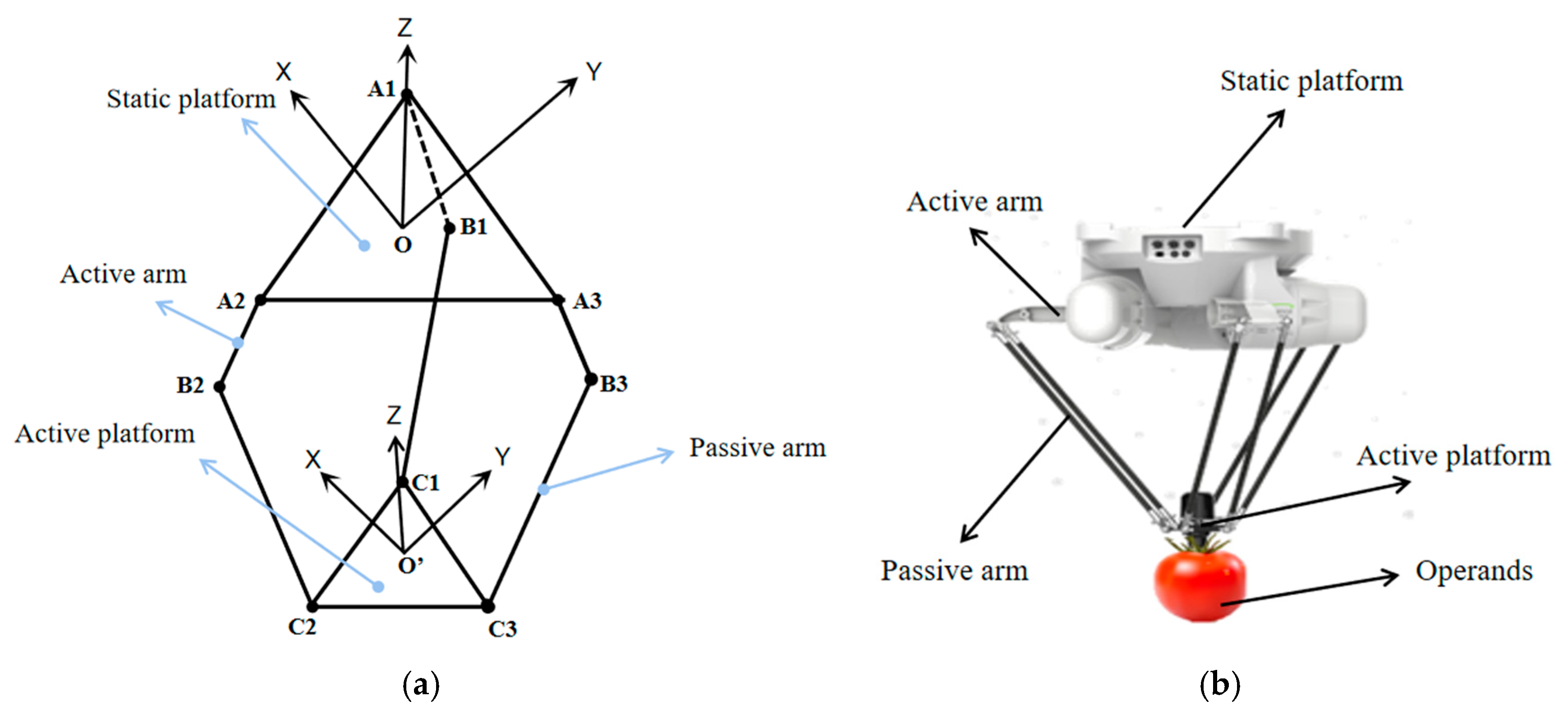
2. Tomato-Grabbing Robot Kinematic Model
2.1. Establishment of Kinematic Equations
2.2. Kinematic Forward Analysis
3. Tomato-Grabbing Robot Path Optimization
3.1. Cartesian Space Path Description
3.2. Joint Space Polynomial Interpolation
4. Optimizing Trajectories Using Enhanced Intelligent Optimization Algorithms
5. Simulation of a Tomato-Grabbing Robot
6. Experimental Validations
7. Conclusions
Author Contributions
Funding
Data Availability Statement
Conflicts of Interest
References
- Castro, T.A.; Leite, B.S.; Assunção, L.S.; de Jesus Freitas, T.; Colauto, N.B.; Linde, G.A.; Otero, D.M.; Bruna Aparecida, S.M.; Camila Duarte, F.R. Red Tomato Products as an Alternative to Reduce Synthetic Dyes in the Food Industry: A Review. Molecules 2021, 26, 7125. [Google Scholar] [CrossRef] [PubMed]
- Cámara, M.; Fernández-Ruiz, V.; Sánchez-Mata, M.; Domínguez Díaz, L.; Kardinaal, A.; van Lieshout, M. Evidence of antiplatelet aggregation effects from the consumption of tomato products, according to EFSA health claim requirements. Crit. Rev. Food Sci. Nutr. 2020, 60, 1515–1522. [Google Scholar] [CrossRef] [PubMed]
- Kumar, M.; Chandran, D.; Tomar, M.; Bhuyan, D.J.; Grasso, S.; Amanda Gomes Almeida, S.; Bruno Augusto, M.C.; Radha Dhumal, S.; Singh, S.; Senapathy, M.; et al. Valorization Potential of Tomato (Solanum lycopersicum L.) Seed: Nutraceutical Quality, Food Properties, Safety Aspects, and Application as a Health-Promoting Ingredient in Foods. Horticulturae 2022, 8, 265. [Google Scholar] [CrossRef]
- Clement, J.; Novas, N.; Gazquez, J.A.; Manzano-Agugliaro, F. High speed intelligent classifier of tomatoes by colour, size and weight. Span. J. Agric. Res. 2012, 10, 314–325. [Google Scholar] [CrossRef]
- Xie, B.; Jin, M.; Duan, J.; Li, Z.; Wang, W.; Qu, M.; Zhou, Y. Design of Adaptive Grippers for Fruit-Picking Robots Considering Contact Behavior. Agriculture 2024, 14, 1082. [Google Scholar] [CrossRef]
- Wang, Z.; Xun, Y.; Wang, Y.; Yang, Q. Review of smart robots for fruit and vegetable picking in agriculture. Int. J. Agric. Biol. Eng. 2022, 15, 33–54. [Google Scholar]
- Wei, D.; Gao, T.; Mo, X.; Xi, R.; Zhou, C. Flexible bio-tensegrity manipulator with multi-degree of freedom and variable structure. Chin. J. Mech. Eng.=Ji Xie Gong Cheng Xue Bao 2020, 33, 1–11. [Google Scholar] [CrossRef]
- Zhao, Y.; Wan, X.; Duo, H. Review of rigid fruit and vegetable picking robots. Int. J. Agric. Biol. Eng. 2023, 16, 1–11. [Google Scholar] [CrossRef]
- Lilge, S.; Nuelle, K.; Childs, J.A.; Wen, K.; Rucker, D.C.; Burgner-Kahrs, J. Parallel-Continuum Robots: A Survey. IEEE Trans. Robot. 2024, 40, 3252–3270. [Google Scholar] [CrossRef]
- Sundaram, R.; Raheman, H.; Paradkar, V. Design and development of a 5R 2DOF parallel robot arm for handling paper pot seedlings in a vegetable transplanter. Comput. Electron. Agric. 2019, 166, 105014. [Google Scholar]
- Yang, H.; Chen, L.; Ma, Z.; Chen, M.; Zhong, Y.; Deng, F.; Li, M. Computer vision-based high-quality tea automatic plucking robot using Delta parallel manipulator. Comput. Electron. Agric. 2021, 181, 105946. [Google Scholar] [CrossRef]
- Hu, X.; Pan, Z.; Lv, S. Picking Path Optimization of Agaricus bisporus Picking Robot. Math. Probl. Eng. 2019, 2019, 8973153. [Google Scholar] [CrossRef]
- Zhao, X.; Cheng, D.; Dong, W.; Ma, X.; Xiong, Y.; Tong, J. Research on the End Effector and Optimal Motion Control Strategy for a Plug Seedling Transplanting Parallel Robot. Agriculture 2022, 12, 1661. [Google Scholar] [CrossRef]
- Zhang, Q.; Zhao, Z.; Gao, G. Fuzzy Comprehensive Evaluation for Grasping Prioritization of Stacked Fruit Clusters Based on Relative Hierarchy Factor Set. Agronomy 2022, 12, 663. [Google Scholar] [CrossRef]
- Zhang, X.; Wang, H.; Rong, Y. Improved inverse kinematics and dynamics model research of general parallel mechanisms. J. Mech. Sci. Technol. 2023, 37, 943–954. [Google Scholar] [CrossRef]
- Zhou, Z.; Gosselin, C. Simplified inverse dynamic models of parallel robots based on a Lagrangian approach. Meccanica 2024, 59, 657–680. [Google Scholar] [CrossRef]
- Wang, J.; Jing, Z.; Guo, J.; Qin, T.; Li, H.; Li, X.; Li, Z.; Meng, F.; Qi, B. A New Theoretical Method for Solving Forward Kinematics of the Parallel Mechanisms Based on Transfer Matrix. Int. J. Aerosp. Eng. 2024, 2024, 2582680. [Google Scholar] [CrossRef]
- Chen, X.; Zhao, H.; Zhen, S.; Liu, X.; Zhang, J. Fixed-time adaptive neural network-based trajectory tracking control for workspace manipulators. Actuators 2024, 13, 252. [Google Scholar] [CrossRef]
- Jia, X.; Zhao, B.; Liu, J.; Zhang, S. A trajectory planning method for robotic arms based on improved dynamic motion primitives. Ind. Robot. 2024; ahead-of-print. [Google Scholar]
- Song, Y.; Li, Q.; Liu, Y.; Wang, L. A Trajectory Planning Method for Capture Operation of Space Robotic Arm Based on Deep Reinforcement Learning. ASME. J. Comput. Inf. Sci. Eng. 2024, 24, 091003. [Google Scholar] [CrossRef]
- Jahanpour, J.; Motallebi, M.; Porghoveh, M. A Novel Trajectory Planning Scheme for Parallel Machining Robots Enhanced with NURBS Curves. J. Intell. Robot. Syst. 2016, 82, 257–275. [Google Scholar] [CrossRef]
- Wang, D.; Zhang, C.; Xi, X. A Novel Interpolation Method for Cutting Trajectories in Spatial Coherent Cutting Machine. J. Phys. Conf. Ser. 2022, 2395, 012033. [Google Scholar] [CrossRef]
- Xu, L.; Su, T. Quintic pythagorean-hodograph curves based trajectory planning for delta robot with a prescribed geometrical constraint. Appl. Sci. 2019, 9, 4491. [Google Scholar] [CrossRef]
- Zhang, X.; Ming, Z. Trajectory Planning and Optimization for a Par4 Parallel Robot Based on Energy Consumption. Appl. Sci. 2019, 9, 2770. [Google Scholar] [CrossRef]
- Myong, S.C.; Jang, K.S.; Kim, Y.H.; Kim, K.H.; Yang, W. An Approach for Elliptical Trajectory Planning with Vertical Straight Line Segments of Pick-and-Place Robot Operation with Height Clearance. Math. Probl. Eng. 2023, 2023, 7419178. [Google Scholar]
- Chen, W.; Liu, J.; Tang, Y.; Huan, J.; Liu, H. Trajectory Optimization of Spray Painting Robot for Complex Curved Surface Based on Exponential Mean Bézier Method. Math. Probl. Eng. 2017, 2017, 10. [Google Scholar] [CrossRef]
- Alfatih, M.F.; Riyadi, M.A.; Setiawan, I. Speed control system in mobile robot based on bezier curve trajectory. IOP Conf. Ser. Mater. Sci. Eng. 2021, 1108, 012015. [Google Scholar] [CrossRef]
- Nguyen, D.H.; Mai, V.L.; Pham, D.P. A Co-Optimization Algorithm Utilizing Particle Swarm Optimization for Linguistic Time Series. Mathematics 2023, 11, 1597. [Google Scholar] [CrossRef]
- Jin, M.; Li, J.; Chen, T. Method for the Trajectory Tracking Control of Unmanned Ground Vehicles Based on Chaotic Particle Swarm Optimization and Model Predictive Control. Symmetry 2024, 16, 708. [Google Scholar] [CrossRef]
- Jiang, Y.; Wang, L. Application of Genetic Algorithm in Optimizing Path Selection in Tourism Route Planning. J. Electr. Syst. 2024, 20, 462–468. [Google Scholar]
- Yu, Y.; Han, J.; Gu, H.; Yang, Y. Dynamic Optimization of Construction Time-Cost for Deep and Large Foundation Pit Based on BIM Technology and Genetic Algorithm. Appl. Sci. 2023, 13, 10716. [Google Scholar] [CrossRef]
- Zeng, X.; Wang, Y. Multi-objective Logistics Distribution Path Optimization Based on Annealing Evolution Algorithm. J. Phys. Conf. Ser. 2023, 2555, 012014. [Google Scholar] [CrossRef]
- Cheng, Y.; Fa-you, A.; Wu, Y.F.; Yan, S.-Q.; Zhu, C.-B.; Zhang, H. Impact of Parameter Tuning with Genetic Algorithm, Particle Swarm Optimization, and Bat Algorithm on Accuracy of the SVM Model in Landslide Susceptibility Evaluation. Math. Probl. Eng. 2023, 2023, 1393142. [Google Scholar]


| Initial Angle (In Degrees) | Cartesian Coordinates (In mm) | ||
|---|---|---|---|
| β1 | β2 | β3 | (x, y, z) |
| 5 | 15 | 20 | (−112.41, −103.44, −928.83) |
| 15 | 25 | 25 | (−215.17, −124.23, −895.11) |
| 40 | 35 | 60 | (46.74, −202.18, −821.16) |
| 60 | 40 | 70 | (165.56, −176.15, −758.52) |
| 70 | 80 | 60 | (−69.67, 125.88, −720.84) |
| 100 | 90 | 80 | (62.53, 108.46, −628.48) |
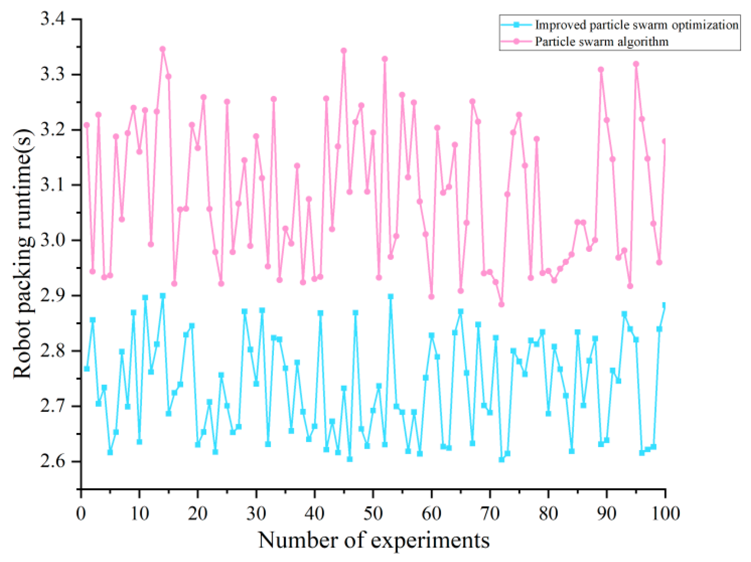
| Iteration | Improved PSO Time (s) | PSO Time (s) |
|---|---|---|
| 1 | 0.65 | 0.78 |
| 2 | 0.71 | 0.80 |
| 3 | 0.69 | 0.76 |
| 4 | 0.73 | 0.84 |
| 5 | 0.66 | 0.72 |
| Average | 0.69 | 0.78 |
Disclaimer/Publisher’s Note: The statements, opinions and data contained in all publications are solely those of the individual author(s) and contributor(s) and not of MDPI and/or the editor(s). MDPI and/or the editor(s) disclaim responsibility for any injury to people or property resulting from any ideas, methods, instructions or products referred to in the content. |
© 2024 by the authors. Licensee MDPI, Basel, Switzerland. This article is an open access article distributed under the terms and conditions of the Creative Commons Attribution (CC BY) license (https://creativecommons.org/licenses/by/4.0/).
Share and Cite
Guo, T.; Li, J.; Zhang, Y.; Cai, L.; Li, Q. Study on Trajectory Optimization for a Flexible Parallel Robot in Tomato Packaging. Agriculture 2024, 14, 2274. https://doi.org/10.3390/agriculture14122274
Guo T, Li J, Zhang Y, Cai L, Li Q. Study on Trajectory Optimization for a Flexible Parallel Robot in Tomato Packaging. Agriculture. 2024; 14(12):2274. https://doi.org/10.3390/agriculture14122274
Chicago/Turabian StyleGuo, Tianci, Jiangbo Li, Yizhi Zhang, Letian Cai, and Qicheng Li. 2024. "Study on Trajectory Optimization for a Flexible Parallel Robot in Tomato Packaging" Agriculture 14, no. 12: 2274. https://doi.org/10.3390/agriculture14122274
APA StyleGuo, T., Li, J., Zhang, Y., Cai, L., & Li, Q. (2024). Study on Trajectory Optimization for a Flexible Parallel Robot in Tomato Packaging. Agriculture, 14(12), 2274. https://doi.org/10.3390/agriculture14122274