Article

Impacts of Geographical Indications on Agricultural Growth and Farmers’ Income in Rural China

1
School of Economics, Shandong Normal University, Jinan 250399, China
2
School of Economics, Shandong University, Jinan 250100, China
3
School of Economics, Shandong University of Finance and Economics, Jinan 250014, China
*
Author to whom correspondence should be addressed.
Agriculture 2024, 14(1), 113; https://doi.org/10.3390/agriculture14010113
Submission received: 11 December 2023 / Revised: 9 January 2024 / Accepted: 9 January 2024 / Published: 10 January 2024
(This article belongs to the Special Issue Application of Machine Learning and Data Analysis in Agriculture)

Abstract

:
Geographical indications (GIs) mitigate information asymmetry in agri-food transactions by providing consumers with origin and quality information. This paper explores the impact of GIs on rural development in China by examining agricultural output and farmers’ income. Utilizing a large county-level dataset and comprehensive official GI information, this study estimates the impact of GIs on agricultural output and rural income using panel-fixed-effects models. The results reveal that GIs significantly boost agricultural added value and rural per capita disposable income. A series of methods, including difference-in-differences, propensity score matching with difference-in-differences, and double machine learning combined with difference-in-differences using random forests verify the robustness of the results. Moreover, by categorizing GIs based on product types, the analysis reveals heterogeneous effects of different GI categories on agricultural growth and income gains for farmers. The research findings in this paper offer valuable insights to inform policymaking aimed at advancing rural development, raising farmers’ incomes, and promoting sustainable agri-food supply chains.

1. Introduction

According to the definition by the World Intellectual Property Organization (WIPO), geographical indications (GIs) are signs used on products that have a specific geographical origin and possess qualities, reputation, or other characteristics that are essentially attributable to that place of origin. They differentiate products based on local natural factors and traditional production methods. Agricultural income is highly dependent on natural conditions which restrict productivity. Commodity crops face inelastic demand and prices, leaving farmers as price takers rather than price setters. The perishable nature of many agricultural goods also weakens farmers’ bargaining positions versus distributors and collectors. However, geographical indications for regional agricultural products can help address these problems by increasing product differentiation and added value. This allows farmers to obtain price premiums on the market, directly boosting income. Successful geographical indications also stimulate local tourism and infrastructure improvement.
According to the UN Food and Agriculture Organization’s 2014 report on GIs: “Adding Value to Agricultural Products, the market share of Cognac brandy was only 1% of global brandy sales in 1960, but exceeded 50% by 2014”. In another report from the French Ministry of Agriculture in 2014, it is estimated that the production and sales of Roquefort blue cheese could help generate around 500 formal job positions in the Aveyron region. In economics, GIs are considered to promote rural development mainly through two mechanisms—reducing information asymmetry and enabling a degree of monopoly power for producers.
Information asymmetry has been extensively studied as a source of market failure in the seminal work by Akerlof [1] on quality uncertainty and adverse selection. This problem is salient in agricultural markets, where intermediaries and distributors understand product attributes better than consumers. Without full information, low-quality goods can crowd out high-quality ones if buyers are unable to differentiate them. Geographical indications have been analyzed as a policy tool to mitigate such inefficiencies. By providing official quality certification based on geographical origin, GIs help convey reliable signals to reduce information gaps between producers and consumers [2,3].
On the other hand, agricultural producers often face high buyer power which depresses their pricing premiums [4]. This results in lower added value, especially in countries where international trade of farm products is relatively restricted [5]. Direct government subsidies have limited effects on addressing this issue and may negatively impact farm survival [6]. GIs as a special form of intellectual property rights confer a degree of monopoly based on geographical origin and product qualities. This increases bargaining power and product added value for farmers [7,8,9], thereby promoting agricultural growth and income in rural regions. While some argue such monopoly effects of GIs may disrupt market competition [10], they can be viewed as correcting inefficiencies caused by information gaps from a welfare economics perspective [3,8,11,12,13]. Furthermore, GIs also increase consumer willingness to pay for certified products [14,15,16], though not always in a Pareto-improving manner [3].
The existing literature on the impacts of GIs in rural areas has focused primarily on several aspects, including agricultural product prices [17,18,19,20], technical efficiency [21,22,23], scale efficiency [24], and agricultural income [25,26,27]. As for impacts on smallholder farmers, Tregear et al. [19] found that GIs can enhance the bargaining power and income distribution of smallholder farmers in global value chains. After GI registration, the planting area and yield per unit area of onions increased, while onion prices rose, resulting in higher farmer incomes. Zhang et al. [27] examined how GIs help reduce urban–rural income disparities from the perspective of agricultural exports. The main mechanisms were increasing value-added products and promoting agricultural structural upgrading in less developed regions.
From a regional perspective, the existing literature has extensively discussed the impacts of GIs on rural development [28,29,30,31,32,33]. As a relatively mature example of geographical indications, most studies have examined the effects of European GIs on agricultural producers [34,35,36,37]. For instance, in Greece, geographical indications can potentially influence value-added products and scarcity through the localization of production, thereby raising farmer income [35]. Kizos et al. [37] analyzed six case studies in Austria, Italy, Greece, and Japan, highlighting the important role of GIs in sharing agricultural information and emphasizing that it should be a process rather than a single step. Some studies have also explored the role of GIs in agricultural development in non-European countries [9,32,33,38,39]. For example, research by Neilson et al. [32] suggests limited impacts of GIs on Indonesia’s coffee farming industry. Similarly, the study by Bowen and Zapata [33] indicates the negative effects of the tequila industry on local economies, owing to the disregard for geographical indications. From the existing literature, it appears that GI systems do not achieve expected outcomes in all countries. As stated, most developing countries “do not have sufficient experience to apply GIs” [40]. Moreover, challenges like limited market differentiation, missing complementary investments, and inadequate legal systems constrain the effectiveness of GIs for inclusive rural development in low-income countries [41].
Among studies related to China, many rely on micro-level survey data to examine GIs’ effects on agricultural growth [42,43,44]. For instance, Deng et al. [42] surveyed producers in Zhejiang and Fujian and found that GIs helped enhance international competitiveness of agricultural products. Zhan and Yu [44] analyzed survey data from 437 households and identified significant impacts of GIs on farmers’ economic benefits. Xue and Yao [43] studied citrus-planting farmers and concluded that GIs promoted agricultural input use and technology adoption.
A summary of relevant references related to this paper is presented in Table 1.
While existing studies have discussed how GIs benefit rural development from multiple angles, some research gaps remain to be explored. First, most works in the literature rely on case studies or small-scale sample surveys, lacking large-scale quantitative empirical evidence. Second, due to data limitations, current research tends to utilize case analyses or micro-level surveys, making it difficult to causally evaluate the treatment effects of GIs on rural development. Finally, existing literature exploring the impact of GIs on rural development in non-European countries remains an area that could benefit from further enrichment. Investigating the influence of GI systems in countries with substantial agricultural populations, such as China and India [45,46], holds positive significance in addressing global poverty challenges.
This study evaluates the impacts of GI registration on rural economic development from the perspectives of agricultural growth and farmer income. Using GI approval data from China’s Ministry of Agriculture and Rural Affairs and county-level economic data from 2010 to 2019, the analysis assesses how GIs promote regional agricultural production and contribute to rural development. To ensure robustness of the effect estimates, causal identification strategies and machine learning techniques are utilized to address endogeneity concerns. The study further investigates heterogeneous effects of GIs across different product categories, offering insights into the optimal targeting of GI policies.
Compared to the existing literature, this study makes several potential contributions. First, it reveals the positive impacts of China’s GI system on both agricultural growth and farmer income using a comprehensive national-level dataset. Most prior studies rely on small-scale surveys of individual GI products, lacking generalizability [25,43,44]. By leveraging macro-level data across counties and years, this research provides more representative evidence on how GI policies reshape regional agricultural development under real-world conditions. The findings can inform national policymaking on scaling up and optimizing China’s GI system.
Second, this study investigates the heterogeneous treatment effects of different types of GIs, including products with different categories of agri-food products. The existing literature rarely compares the development impacts of GIs across products, representing a significant research gap [47,48]. The product-specific estimates generated in this study reveal how GI effectiveness varies based on product attributes. The results provide insights into prioritizing GI development policies by product category to maximize rural income growth.
Third, this research contributes to the existing literature on geographical indications (GIs) in China. As a representative country in East Asia, China exemplifies a variety of agriculture-dependent nations. In contrast to several studies on GIs and rural development in European countries [7,30], this research addresses a knowledge gap by quantifying the impact of GIs on agricultural and income growth in rural China. Given China’s prominence as a major GI producer, the findings provide valuable insights for policymaking, offering guidance on how to leverage GIs and intellectual property tools to foster inclusive development in countries like China.
The remaining content of this paper is structured as follows: Section 2 provides an introduction to the background, data, methods, and design of the research. Section 3 reports the results of empirical tests, including baseline regression and causal inference, robustness checks using machine learning, and further analysis based on the classification of geographical types. Section 4 summarizes the conclusions of the study and initiates discussions, along with offering policy recommendations.

2. Materials and Methods

2.1. Research Background and Hypotheses

Geographical indications (GIs) were first legally protected in China in the 1990s. With China’s accession to the WTO in 2001, the legislation and approval of GIs accelerated. The State Administration for Industry and Commerce, the General Administration of Quality Supervision, Inspection and Quarantine, and the Ministry of Agriculture are the main governmental agencies that formulated regulations and granted GI certification. While progress was slow before 2005, the number of approved GIs grew rapidly afterward, exceeding 1000 by 2012. Promoting GIs has since been an important aspect of China’s rural revitalization policies. As of today, China has the most GI products globally, demonstrating the vital role of GIs in boosting regional brands and rural development.
The data on geographical indications for agricultural products used in this study were obtained from the China Green Food Center, an association affiliated with the Chinese Ministry of Agriculture. The dataset records the date of registration, product name, province, certificate holder, product type, and certificate number for each geographical indication of the agricultural products. Unlike the geographical indications for processed products published by the Intellectual Property Office, all of the GI products included in this dataset are unprocessed primary agricultural goods.
Table 2 summarizes the number of new GIs granted annually during this period across product categories. Fruit, cereal crops, and vegetables and edible fungi have the most certified GIs. The annual number of new GIs fluctuated, with rapid growth before 2010 and some volatility in the years after. By 2021, the total number of agricultural GIs reached 3430.
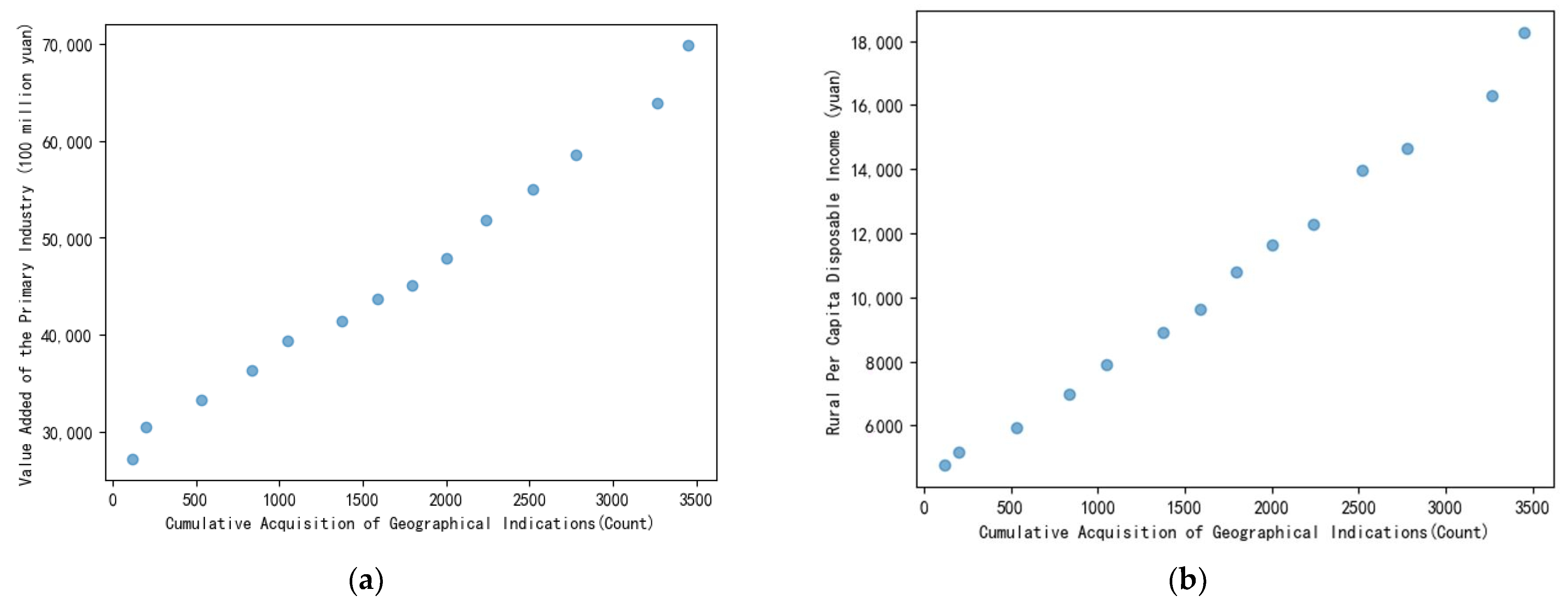
Theoretically, by protecting the reputation of agricultural products from specific regions, geographical indications can endow products with brand value and recognition. This allows producers to charge premium prices and stimulates market demand, thereby increasing agricultural added value and farmers’ income in corresponding regions.
To examine whether this mechanism is empirically observable at the national level, we visualized the aggregate relationships using scatter plots. Figure 1a,b depict the cumulative numbers of agricultural GIs versus China’s agricultural added value and rural per capita disposable income during 2008–2021.The scatterplot shapes indicate a strong positive correlation between the cumulative number of GIs obtained and each respective indicator, with the data points forming an approximate linear relationship: regions with higher total acquired GIs tended to have greater agricultural added value and rural income growth at the national level, as evidenced by the close to linear trend lines. Therefore, we further contemplate whether this relationship is generally prevalent at a more detailed level, forming the starting point for the research questions addressed in this paper.

2.2. Data Sources

This study utilizes data from multiple sources. The data on agricultural GIs were obtained from the public reports of approved GIs published by the Chinese Ministry of Agriculture (MOA). Specifically, the Green Food Association, affiliated with MOA, releases on its official website the registration information for all agricultural GIs in China, including the GI name, authorized unit, and product category. In this paper, the original data was preprocessed using Python 3.7 and the models were built and analyzed using STATA 16.0.
The outcome variables of agricultural added value and rural disposable income per capita are from the China County Statistical Yearbooks. Control variables related to geographic, climate, fiscal, industrial, and agricultural conditions also come from the yearbooks.
To alleviate endogeneity concerns, alternative data are used to construct instrumental variables. The provincial cumulative GI numbers are calculated based on the Intellectual Property Office’s approval announcements. The average cumulative GI counts of neighboring counties are derived from the geospatial relationships between counties.
By matching the GI data with the statistical yearbooks, a comprehensive county-level panel dataset is compiled for the empirical analysis. The sample covers 1731 counties from 2000 to 2019. Several validation checks are conducted to recheck the accuracy of data from the local government annual reports, ensuring the accuracy and consistency of the combined data from multiple sources.
The use of authoritative statistical yearbooks provides reliable county-specific observations. The panel structure enables controlling unobserved heterogeneity. The expansive coverage offers significant variations across regions and GI categories for identification. Data processing and integration are conducted carefully to guarantee data quality for rigorous empirical examination.

2.3. Model Specification

The central inquiry of this study revolves around assessing the impact of cumulative acquisitions of GIs on agricultural growth and rural income. To effectively tackle this multifaceted question, we employ a panel-fixed-effects model. This approach is particularly advantageous as it helps control for unobservable time-invariant factors that could confound the relationship between GIs and agricultural outcomes. By doing so, it allows us to isolate the treatment effect of GIs more effectively. The specific model is as follows:
o u t c o m e i t = β 0 + β 1 G I i t + β m X i t + μ i + τ t + ε i t
In the equation, o u t c o m e i t represents the outcome variable, which corresponds to either the agricultural added value or the per capita disposable income of rural areas in each county or district. β 0 is the intercept; G I i t represents the cumulative acquisition of GIs for agricultural products; β 1 is the estimated coefficient for the treatment effect; X i t is the set of control variables with β m as the vector of their estimated coefficients. Although this study attempts to control for the set of variables that may simultaneously affect the dependent variable and the core explanatory variable, it is challenging to entirely eliminate endogeneity issues resulting from omitted variables. To address this, the study controls for individual fixed-effects μ i at the county or district level to account for individual factors that do not change over time, and time-fixed-effects τ t to control for time-related factors that do not vary across individuals. ε i t represents the random error term in the model.
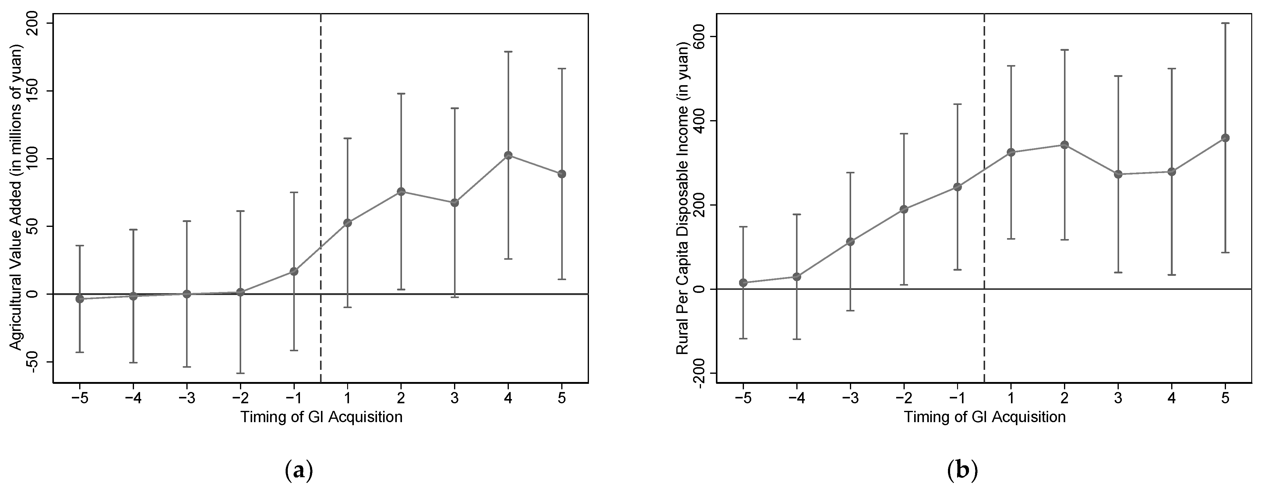
Furthermore, recognizing that GI acquisitions constitute events with lasting consequences and are influenced by relatively exogenous factors such as county-level natural environments, historical contexts, and cultural influences, we also employ the difference-in-differences (DID) method in robustness parts. DID offers several distinct advantages. It provides a framework to identify causal relationships by comparing changes in outcomes between the treatment group (counties acquiring GIs) and control group (those not acquiring GIs) over time. It can also account for potential time-varying confounding factors. This DID approach can strengthen causal inference and provide insights into the long-term effects of GIs. The specific model for identifying the treatment effect is as follows:
o u t c o m e i t = β 0 + β 1 T r e a t i × P o s t t + β m X i t + μ i + τ t + ε i t
Unlike Equation (1), in Equation (2), the core explanatory variable is replaced with a DID term (as T r e a t i × P o s t t above) representing the cumulative acquisition of GIs by counties or districts. In other words, if a county or district has ever acquired a GI in any year, then T r e a t i takes the value of 1, otherwise it takes the value of 0; P o s t t is the dummy variable representing whether a county or district gained any GI in year t, since the value will take 1 from that year onward. Control variables are added to the treatment effect identification model to ensure that the model satisfies the parallel trends assumption. Additionally, individual and time fixed effects are controlled to mitigate the impact of omitted variable bias.
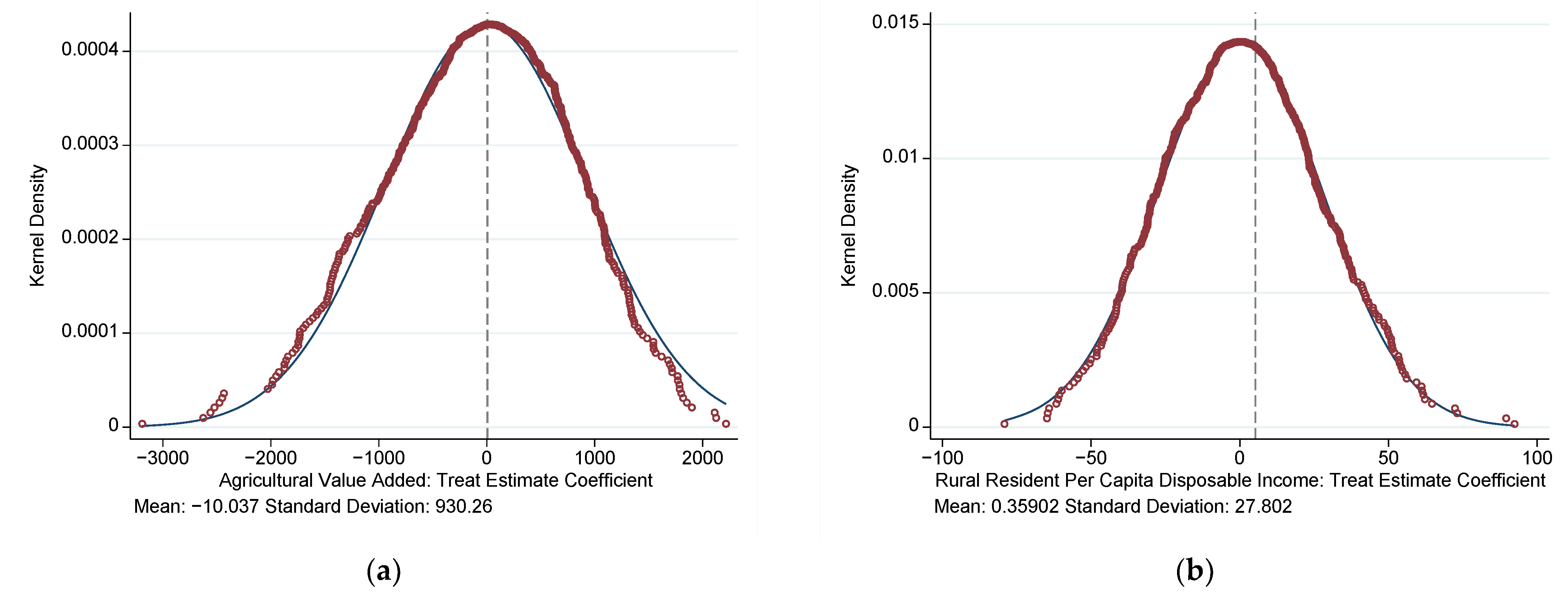
However, it is important to acknowledge the limitations of DID, particularly when dealing with multiple time points and potential non-linearity in the treatment effect. To address these limitations and further enhance the precision of our estimations, we leverage the double/debiased machine learning (DML) approach. The DML method, as proposed by Chernozhukov et al. [49], leverages the advantages of machine learning models in high-dimensional data to control confounding factors’ interference with treatment effects [6]. This results in more unbiased estimates, reduced estimation variance, increased estimation accuracy, and greater flexibility in relaxing the linear treatment effect assumption of the model. By doing so, DML provides more unbiased estimates, reduces estimation variance, and offers greater flexibility in modeling the treatment effect, thereby allowing us to capture nuanced relationships between GIs and agricultural growth as well as income levels in rural areas.
To elucidate its fundamental principles, the DML method utilizes the example of the partially linear model as follows:
Y = α∙D + g(X) + U
D = m(X) + V
In the above equations, after controlling for confounding covariate set g ( X ) , whose functional form does not necessarily have to be linear, α represents the estimated coefficient for the treatment variable D , which is the main estimation objective of this method. m ( X ) denotes the conditional expectation of the treatment effect given the covariate set, i.e., E [ D | X ] . U and V are both random error terms. Specifically, DML divides the dataset into two parts: one for estimating interference terms and the other for estimating treatment effects and structural parameters. Modern machine learning methods, such as random forests, are used to estimate interference terms, including E [ Y | X ] and E [ D | X ] . Subsequently, the estimated interference terms are used to eliminate estimation bias for treatment effects and structural parameters. Finally, semi-parametric methods like local linear regression or kernel regression are employed to estimate treatment effects and structural parameters. Compared to traditional statistical methods, DML offers the advantages of relaxing the linearity assumption of the DID model, the parallel trends assumption, and provides more unbiased and efficient estimates.

2.4. Variable Selection

The key explanatory variable is the cumulative number of agricultural GIs at the county level, which measures the total GIs obtained in each county by each year. The outcome variables are the annual agricultural added value and rural per capita disposable income for each county.
The core explanatory variable is the cumulative number of agricultural GIs at the county level in China during 2000–2019. The dataset only provides information on the province for each GI product, without specifying the district or county. In order to match the GI information to the district and county levels, we use text analysis to extract the geographical information from the product name and certificate holder name. We then query the corresponding 6-digit administrative code to use as the identifier. The panel data of cumulative GI counts and approval years are constructed for each county.
To account for confounding factors, control variables that may affect both GI adoption and outcomes are included in the regressions. Natural conditions like temperature, humidity, and precipitation determine the types of agriculture and thus may influence GI application and productivity. Agricultural machinery power reflects infrastructure conditions. Fiscal expenditures and the number of towns/villages represent government institutional factors. These controls are relatively stable and unlikely to be influenced by reverse causality.
The machine learning methods in this study incorporate a comprehensive set of covariates, including major indicators from the China County Statistical Yearbooks that can potentially affect both GI adoption and outcomes. On one hand, the high-dimensional covariate space allows machine learning models like random forests to partition the feature space in more dimensions, better isolate the effects of GIs, and reduce omitted variable bias. This flexibility relaxes the strict exogeneity assumptions in linear models. On the other hand, high dimensionality risks overfitting a particular dataset. To address this, ensemble approaches are used to aggregate predictions from different decision trees and improve out-of-sample prediction. Cross-validation further enhances generalizability by evaluating performance on held-out subsets.
Summary statistics of the main variables are presented in Table 3. The sample covers 1731 counties from 2000 to 2019, with over 20,000 observations. There is substantial variation in GIs obtained across counties and over time during the sample period.

3. Results

3.1. Baseline Regressions

In this study, we commence by conducting baseline regressions based on Equation (1). The estimation results are presented in Table 4, entries (1) to (4). Entries (1) and (2) correspond to regression results with the agricultural added value in various counties as the dependent variable. Entry (1) represents the univariate regression, while entry (2) adds control variables to the model. The estimation outcomes reveal a significant positive impact of obtaining geographical indications for agricultural products on the primary industry added value in counties. On average, each acquisition of a geographical indication is associated with an increase of CNY 58.98 million in the primary industry added value, and this effect is statistically significant at the 1% level.
Entries (3) and (4) similarly represent univariate and control-variable-added regressions, respectively, with rural residents’ per capita disposable income as the dependent variable. The results indicate that obtaining a geographical indication for agricultural products is associated with an increase of CNY 161.5 in rural residents’ per capita disposable income, and this effect is statistically significant at the 5% level. Notably, all these estimations control for individual fixed effects and time fixed effects, and cluster the standard errors at the county level. Based on the findings presented in Table 4, this study provides empirical support for research hypothesis 1.

3.2. Robustness Checks

3.2.1. Mitigating Endogeneity Using Instrumental Variables

To mitigate endogeneity concerns arising from reverse causality, this study employs the average cumulative GI count of neighboring counties as an instrumental variable for the core explanatory variable. The number of GIs obtained in nearby counties is likely correlated with that in the target county due to potential demonstration effects. However, it may not directly influence the county’s agricultural added value, thus helping to satisfy the relevance and exogeneity conditions for a qualified instrument.
Table 5 (1)–(3) report the instrumental variable regression results. Entry (1) presents the first-stage regression, showing that the instrument is a significant predictor of the potentially endogenous GI variable, with the F-statistic exceeding the threshold of 10. Entry (2) reports the second-stage regression results. Compared to the baseline model, the coefficient for cumulative GI count is substantially larger at CNY 89.6736 million and remains significant at the 10% level. The table also reports weak instrumental variable tests, Kleibergen–Paap LM statistics, under the Wald F-statistic identification, and their corresponding critical values for a 10% sample. The results indicate that this estimation rejects the hypotheses of weak instruments and under identification, providing evidence for the effectiveness of the instrumental variable. Furthermore, when both the instrument and GI variable are included in the regression as shown in Entry (3), the instrument itself becomes statistically insignificant. This offers evidence that the instrumental variable satisfies approximate exogeneity.
A similar procedure is followed for rural income per capita as the dependent variable, using provincial cumulative GI count as the alternative instrument. Entries (4)–(6) present the regression results, demonstrating that the instrument is statistically strong and the GI variable has a positive, significant effect on rural income after instrumenting.
The divergence in the instrumental variable regression results compared to the baseline estimates can be largely attributed to the choice of instruments. For the neighboring counties’ average GI, its agricultural conditions are more similar, leading to a higher correlation with the treatment variable. This results in a second-stage coefficient that is closer in magnitude to the regression of outcome on instrument, with an increase of around 1.75 times. In contrast, the provincial cumulative GI has a much lower correlation, resulting in a larger final estimate due to the smaller first-stage coefficient. The adoption of two distinct instruments, considering issues like weak instruments, reflects that the baseline estimate is not overestimated.

3.2.2. Re-Estimating the Treatment Effects Using Staggered DID Model

In the context of this research question, the quantity of agricultural geographical indications obtained can be considered a relatively exogenous factor. This is because its approval is constrained by various exogenous factors, such as historical and cultural factors, as well as unique natural conditions. Hence, this study also attempts to estimate the treatment effects of geographical indications using the staggered DID model. Unlike the baseline regression, in this section, we transform the cumulative acquisition of geographical indications in each county into a binary variable, denoted as “treat”. Specifically, for a county that first obtains geographical indications in a certain year and subsequent years, treat takes the value of 1; otherwise, it takes the value of 0. We then estimate Equation (2) accordingly.
The estimated results are presented in Table 6, as shown in (1) and (2). Compared to the baseline regression, the regression coefficients of the GI dummy variables for both the agricultural added value and rural residents’ per capita disposable income increased, and both are statistically significant at the 5% level. Compared to the baseline regression, the estimation results of the DID regression no longer represent the marginal effect of adding each GI, but rather the average treatment effect of obtaining GI on agricultural output and farmer income.
An important assumption of the difference-in-differences model is the parallel trends assumption, which requires the treatment and control groups to exhibit similar trends prior to treatment. To examine this, we follow the approach by Beck et al. [50] to construct lead and lag variables indicating five periods before and after the actual treatment period. These variables are substituted into model (2) in place of the treatment dummy. To avoid multicollinearity, we omit the period when treatment actually occurred. By graphing the 95% confidence intervals of the lead/lag coefficient estimates, we can visualize whether parallel trends hold for the two outcome variables. As shown in Figure 2a,b, the regressions include the same control variables as the baseline model.
Figure 2a presents the parallel trend test results for agricultural added value (scaled to million yuan). The lag coefficients before treatment are statistically insignificant from zero, suggesting parallel trends hold. After treatment occurs, the coefficients become significantly positive, reflecting the positive effect of GIs. Figure 2b shows a similar pattern for rural income, although income starts responding to treatment from lags 1 and 2 before treatment happens. The explanation for this phenomenon is that some high-quality agricultural products may already have a certain level of fame prior to obtaining a GI, which causes the treatment effect to lag, and farmers’ incomes start to increase before they receive the treatment. However, this result is exactly consistent with the purpose of our study, which is to argue that “geographical indications can increase product popularity and thus improve farmers’ income through increased sales”. If some of the products have a certain degree of awareness before obtaining a geographical indication and can improve farmers’ income, then it is also an explanation for the rationality of the existence of the geographical indication system. Although this phenomenon does not contradict the research purpose of this paper, we will continue to try to control confounders affecting the conditional parallel trend using the DML-DID method to mitigate the interference with the estimation. Overall, the graphical analysis provides evidence on the satisfied or close-to-satisfied parallel trends assumption.
We further conducted a placebo test on the treatment effect of GIs. Specifically, we randomly shuffled the treated counties and treatment timing, then re-estimated model (2) with these artificial treatments. Figure 3a,b show the kernel density plots of the placebo treatment effects from 500 repetitions. As the distribution of the difference-in-differences coefficients for the placebo treatments center around zero in the figures, the Z-statistics of both plots are not statistically significant from zero. This randomized permutation test provides evidence that the true effect of GIs on the outcome variables is meaningful rather than a spurious artifact. Both regressions successfully pass this placebo test, lending credibility to the identification strategy.

3.2.3. Reducing Selection Bias and Endogeneity Using PSM-DID Method

Sample selection bias could be another source of estimation error, as counties may differ in geographic, economic, and cultural characteristics. This affects the comparability between treatment and control groups. The Propensity Score Matching-Difference-in-Differences (PSM-DID) method integrates propensity score matching with difference-in-differences analysis to address selection bias and endogeneity concerns by matching treated and control groups before conducting difference-in-differences analysis.
We use the same set of control variables from the baseline model and logit models to predict each county’s propensity score of receiving treatment based on these covariates. A ratio of 1:1 nearest neighbor matching with a caliper of 0.05 is performed to pair each treated unit with a control. Equation (2) is then re-estimated on the matched sample.
Figure 4a–d present covariate balance checks and common support frequencies before and after matching. The matching process substantially improves balance and yields a relatively equal number of treated and control units satisfying common support.
Table 6’s entries (3) and (4) show the PSM-DID results. The coefficient for the DID term decreases slightly for agricultural added value but increases for rural income compared to columns (1) and (2). Both remain statistically significant. This robustness check accounting for sample selection provides evidence that the positive effects of GIs remain significant.

3.2.4. Mitigating Limitations of DID Estimation Using DML-DID Approach

Machine learning methods can relax the linear functional form and parallel trends assumptions imposed by previous robustness checks. By flexibly estimating the nuisance functions, machine learning can reduce bias from covariates and model misspecification. This part implements a double machine learning difference-in-differences (DML-DID) approach using the DDML command in STATA 16.0 by following the below steps.
First, a partially linear model is initialized with county clusters and 5-fold cross-validation. Second, random forests are used to estimate the conditional expectations E [ Y | X ] and E [ D | X ] , given the set of covariates. The hyperparameters are set at 100 trees. Third, cross-validation is performed to estimate the conditional expectations. Fourth, the parameter of interest and structural parameters are estimated using semi-parametric techniques.
Unlike linear regression, tree-based methods select covariates based on information theory to best partition the outcome variable. This makes random forests more robust to raw data issues and flexible functional forms. The ensemble and cross-validation further improve generalizability. A wide set of indicators from the China County Statistical Yearbooks are included as covariates to reduce omitted variable bias but avoid overfitting.
As shown in Table 6, entries (5) and (6), the DML-DID model yields noticeably larger estimated effects of GIs on the two outcome variables compared to the baseline linear specifications, while remaining statistically significant. This provides evidence that the positive impacts are unlikely to be overestimated, enhancing confidence in the results.

3.2.5. Using Log-Transformed Dependent Variable to Measure Relative Effects

The use of a log-linear model with logarithmic transformation of the explanatory variables allows for an approximate estimation of the treatment effect of GIs on agricultural added value and rural disposable income. For this purpose, we logarithmized these two explanatory variables and re-estimated models (1) and (2), respectively, with the estimated results shown in Table 6, entries (1)–(4).
The estimation results in Table 7 show that GIs remain statistically significant for the two log-transformed explanatory variables. Each additional GI captured can increase a district’s agricultural added value by an average of 2.47% and increase per capita income by 0.78% on average. Estimates under the DID model are even higher, with access to GIs increasing agricultural added value in a district by 4.38% on average and per capita income by 1.9% on average.

3.3. GI Effects on Agricultural Added Value: Via Various Product Categories

This section examines the heterogeneous effects of cumulative GIs on agricultural added value across different product categories. Among the 18 categories, 13 with observations for over 10 counties are analyzed, including cereals, vegetables and fungi, fruits, oil crops, sugar crops, aquatic products, meat, dairy, eggs, cotton, tobacco, tea, and spices.
Separate regressions are estimated with the cumulative GI count for each category as the explanatory variable and agricultural output as the outcome, controlling county and year fixed effects. Table 8 summarizes the key coefficient for the GI variable in entries (1)–(13).
The results show that obtaining additional GIs has statistically significant positive effects on agricultural added value for vegetables and fungi, fruits, aquatic products, dairy, cotton, and tobacco. The top three categories with the largest coefficients are cotton, tobacco, and aquatic products. In contrast, GIs for oil crops, meat, and eggs do not have significant impacts. Notably, more GIs for sugar crops, tea, and spices exhibit negative effects, likely because further processing dilutes the value share of raw agricultural output for these sectors.
Overall, the heterogeneity analysis provides nuanced evidence that GIs influence agricultural productivity in a product-specific manner. Targeted GI development policies may be warranted for strategic sectors.

3.4. GI Effects on Rural per Capita Disposable Income: Via Various Product Categories

Similarly, this section estimates the heterogeneous effects of GIs by product category on rural per capita disposable income. As shown in Table 9, obtaining more GIs has statistically significant positive impacts on rural income for fruits, sugar crops, aquatic products, dairy, and tobacco. The income growth is most pronounced for sugar, tobacco, dairy, aquatic products, and tea. Notably, fruits, aquatic products, dairy, and tobacco GIs promote both agricultural added value and rural income significantly. Although sugar and tea GIs do not increase agricultural output significantly, they still boost rural income substantially. In contrast, more GIs for spices lower both outcomes, implying resource misallocation where primary products fail to provide sufficient added value. For cereals, vegetables and fungi, oil crops, meat, eggs, and cotton, the estimated effects of GIs on rural income are insignificant.

4. Conclusions and Discussion

As an important factor influencing the supply and demand of agricultural products, the geographical indication system also plays a vital role in rural development and is of great significance with regard to policies in raising farmer incomes, boosting agricultural added value, and maintaining stability in agricultural supply chains. By leveraging nationally representative county-level data and rigorous econometric approaches, this study helps bridge the knowledge gap and demonstrates the substantial impact of GIs on promoting agricultural and rural growth in China. Synthesizing the analysis conducted in this paper, several meaningful conclusions can be drawn.
Firstly, the results of this study illustrate a noteworthy effect—the acquisition of GIs for agricultural products significantly enhances the per capita disposable income of farmers. On average, every additional geographical indication acquired in China’s counties and districts boosts agricultural added value by CNY 58.97 million, which translates to an increase of CNY 162 per capita disposable income for local farm households. This finding is consistent with the research conducted by Zhang et al. [27], which also suggests that securing GIs can mitigate the income disparities between urban and rural areas, representing an alternative facet of bolstering farmers’ income. Nevertheless, it is essential to note a divergence between this study and Zhang et al.’s [27] research. While Zhang et al. employed provincial-level data, our study employs county-level data, offering a finer level of granularity. This finer resolution permits a more accurate identification of treatment effects, thus better mitigating the potential influence of economic fluctuations and non-agricultural factors on the observed treatment effects.
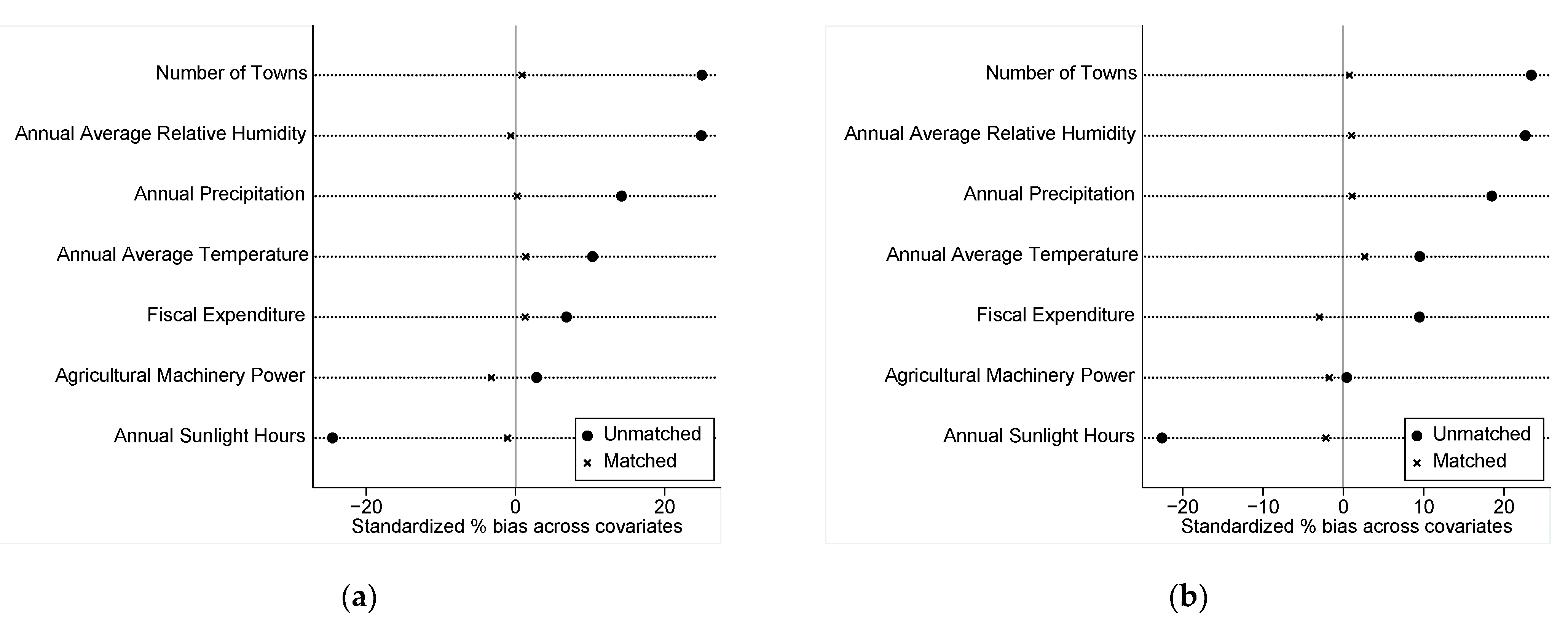
Secondly, treating access to GIs as an exogenous shock and estimating the results after GI access relative to without or before access shows that this treatment effect boosts agricultural output by CNY 106.43 million and per capita disposable income by CNY 347, respectively. The estimates from matching similar counties and districts as a control group based on natural conditions and the size of economy are also closer in value. Using the DML-DID method, the estimates become substantially higher when random forest estimation replaces linear regression to mitigate endogeneity from omitted variables. The DML-DID models estimate that agricultural output increases by CNY 142.76 million and per capita disposable income rises by CNY 581. This suggests that the impact of GIs on rural development is relatively robust. Given the limited set of covariates, the true uplift from GIs may be even greater than estimated in this paper.
Thirdly, this study conducts a cross-category comparison of different types of GIs to uncover their heterogeneous treatment effects on agricultural added value and per capita income in area. The results reveal noticeable variations in the economic impacts across GI categories. For instance, the acquisition of GIs for vegetables and fungi, fruits, aquatic products, dairy, cotton, and tobacco demonstrates the most pronounced positive effects on agricultural productivity. In contrast, obtaining geographical indications for highly processed crops such as sugar and tea has negative effects on agricultural added value but increases farmers’ income. The possible reason is that such geographical indications enhance the added value of these products, specifically the prices of raw materials. Traditional farmers, who were originally reliant on local enterprises for cooperative production, are now more inclined to invest in processing production due to the price changes brought about by geographical indications. This signifies an increase in vertical integration, aligning with the findings of [31]. The rise in prices of raw material products leads to an increase in production costs, which is one of the potential reasons for the decrease in agricultural added value. However, from the perspective of increased farmer income, this is not considered a negative impact. Overall, these findings provide strong evidence on the necessity of developing tailored policies based on the unique characteristics and industrial contexts of different GI products, which are consistent with [51].
While this study provides novel evidence on the positive effects of GIs using rigorous methods, it has some limitations that could be addressed in future research. First, due to data limitations, we are unable to precisely identify the contribution of each GI category to agricultural output. This means the estimates in this paper may still face some confounding from unobserved factors. Second, due to the relatively small number of GI infringement cases in China, which totaled only four nationwide as of August 2023, we are unable to assess the impact of government efforts to protect GIs on rural development. Third, dynamic and lagged effects of GIs deserve further investigation with time-series techniques. Lastly, other factors like cultural effects and promotional efforts may also play a role.
Despite these limitations, this study offers several meaningful policy implications. First, the regulatory oversight and promotion for strategic GI products with significant agricultural returns should be strengthened, such as vegetables, fruits, and aquatic products. Second, misallocation issues in certain processed crop GIs need to be addressed to realize their potential. Third, balancing the interests across all stages of the industry value chain is essential, especially for processed products. Fourth, standardized benefit sharing and enforcement mechanisms for different GI categories can be considered. Fifth, localized GI development plans should be formulated based on regional contexts and strengths. Ultimately, this study provides strong empirical support for optimizing China’s GI system and policies to drive sustainable rural development.

Author Contributions

Conceptualization, X.Y.; methodology, X.Y. and J.L. (Jia Li); software, X.Y. and R.C.; validation, J.L. (Jianxu Liu); formal analysis, X.Y. and S.X.; investigation, S.X. and R.C.; resources, J.L. (Jianxu Liu); data curation, R.C. and J.W.; writing—original draft preparation, X.Y.; writing—review and editing, J.W.; visualization, R.C.; supervision, J.L. (Jia Li); project administration, J.L. (Jia Li); funding acquisition, J.L. (Jia Li) and X.Y. All authors have read and agreed to the published version of the manuscript.

Funding

This research was funded by the Shandong Provincial Social Science Planning Research Project (Grant No. 21CJJJ31) sponsored by the Shandong Provincial Office of Philosophy and Social Sciences.

Institutional Review Board Statement

Not applicable.

Data Availability Statement

The data presented in this study are available on request from the first author.

Acknowledgments

We sincerely thank the editor and the reviewers for their helpful comments and suggestions about our manuscript.

Conflicts of Interest

The authors declare no conflict of interest.

References

  1. Akerlof, G.A. The market for “lemons”: Quality uncertainty and the market mechanism. In Uncertainty in Economics; Elsevier: Amsterdam, The Netherlands, 1978; pp. 235–251. [Google Scholar]
  2. Anania, G.; Nisticò, R. Public regulation as a substitute for trust in quality food markets: What if the trust substitute cannot be fully trusted? J. Institutional Theor. Econ. JITE Z. Gesamte Staatswiss. 2004, 160, 681–701. [Google Scholar] [CrossRef]
  3. Zago, A.M.; Pick, D. Labeling policies in food markets: Private incentives, public intervention, and welfare effects. J. Agric. Resour. Econ. 2004, 29, 150–165. [Google Scholar]
  4. McCorriston, S.; Morgan, C.W.; Rayner, A.J. Processing technology, market power and price transmission. J. Agric. Econ. 1998, 49, 185–201. [Google Scholar] [CrossRef]
  5. Maertens, M.; Minten, B.; Swinnen, J. Modern food supply chains and development: Evidence from horticulture export sectors in Sub-Saharan Africa. Dev. Policy Rev. 2012, 30, 473–497. [Google Scholar] [CrossRef]
  6. Key, N.; Roberts, M.J. Government payments and farm business survival. Am. J. Agric. Econ. 2006, 88, 382–392. [Google Scholar] [CrossRef]
  7. Belletti, G.; Marescotti, A.; Sanz-Cañada, J.; Vakoufaris, H. Linking protection of geographical indications to the environment: Evidence from the European Union olive-oil sector. Land Use Policy 2015, 48, 94–106. [Google Scholar] [CrossRef]
  8. Teuber, R. Consumers’ and producers’ expectations towards geographical indications: Empirical evidence for a German case study. Br. Food J. 2011, 113, 900–918. [Google Scholar] [CrossRef]
  9. Biénabe, E.; Marie-Vivien, D. Institutionalizing geographical indications in southern countries: Lessons learned from Basmati and Rooibos. World Dev. 2017, 98, 58–67. [Google Scholar] [CrossRef]
  10. Hughes, J. Champagne, feta, and bourbon: The spirited debate about geographical indications. Hastings LJ 2006, 58, 299. [Google Scholar]
  11. Lence, S.H.; Marette, S.; Hayes, D.J.; Foster, W. Collective marketing arrangements for geographically differentiated agricultural products: Welfare impacts and policy implications. Am. J. Agric. Econ. 2007, 89, 947–963. [Google Scholar] [CrossRef]
  12. Mérel, P.; Sexton, R.J. Will geographical indications supply excessive quality? Eur. Rev. Agric. Econ. 2012, 39, 567–587. [Google Scholar] [CrossRef]
  13. Moschini, G.; Menapace, L.; Pick, D. Geographical indications and the competitive provision of quality in agricultural markets. Am. J. Agric. Econ. 2008, 90, 794–812. [Google Scholar] [CrossRef]
  14. Bienenfeld, J.M. Consumer Willingness to Pay for Organic, Environmental and Country of Origin Attributes of Food Products; The Ohio State University: Columbus, OH, USA, 2014. [Google Scholar]
  15. Lusk, J.L.; Roosen, J.; Shogren, J. The Oxford Handbook of the Economics of Food Consumption and Policy; Oxford University Press: Oxford, UK, 2011. [Google Scholar]
  16. Feldmann, C.; Hamm, U. Consumers’ Perceptions and Preferences for Local Food: A Review. Food Qual. Prefer. 2015, 40, 152–164. [Google Scholar] [CrossRef]
  17. De Roest, K.; Menghi, A. Reconsidering ‘traditional’ food: The case of Parmigiano Reggiano cheese. Sociol. Ruralis 2000, 40, 439–451. [Google Scholar] [CrossRef]
  18. Gerz, A.; Dupont, F. Comté cheese in France: Impact of a geographical indication on rural development. Orig.-Based Prod. Lessons Pro-Poor Mark. Dev. Bull. 2006, 372, 75–87. [Google Scholar]
  19. Tregear, A.; Török, Á.; Gorton, M. Geographical indications and upgrading of small-scale producers in global agro-food chains: A case study of the Makó Onion Protected Designation of Origin. Environ. Plan. A 2016, 48, 433–451. [Google Scholar] [CrossRef]
  20. Hajdukiewicz, A. European Union agri-food quality schemes for the protection and promotion of geographical indications and traditional specialities: An economic perspective. Folia Hortic. 2014, 26, 3. [Google Scholar] [CrossRef]
  21. Iraizoz, B.; Bardají, I.; Rapún, M. Do ‘protected geographical indications’(PGI)-certified farms perform better? The case of beef farms in Spain. Outlook Agric. 2011, 40, 125–130. [Google Scholar] [CrossRef]
  22. Sellers-Rubio, R.; Más-Ruiz, F.J. Economic efficiency of members of protected designations of origin: Sharing reputation indicators in the experience goods of wine and cheese. Rev. Manag. Sci. 2015, 9, 175–196. [Google Scholar] [CrossRef]
  23. Bouamra Mechemache, Z.; Chaaban, J. Determinants of adoption of protected designation of origin label: Evidence from the french brie cheese industry. J. Agric. Econ. 2010, 61, 225–239. [Google Scholar] [CrossRef]
  24. Dimara, E.; Pantzios, C.J.; Skuras, D.; Tsekouras, K. The impacts of regulated notions of quality on farm efficiency: A DEA application. Eur. J. Oper. Res. 2005, 161, 416–431. [Google Scholar] [CrossRef]
  25. Delattre, F.; Hauwuy, A.; Perron, L. The AOC label for Savoyard cheeses: Past dynamics, achievements and challenges in the today’s changing context (CAP, urban development). Rev. Géogr. Alp. 2005, 93, 119–126. [Google Scholar] [CrossRef]
  26. Barjolle, D.; Paus, M.; Perret, A.O. Impacts of Geographical Indications-Review of Methods and Empirical Evidences. In Proceedings of the 2009 Conference, Beijing, China, 16–22 August 2009. [Google Scholar]
  27. Zhang, S.; Sun, Y.; Yu, X.; Zhang, Y. Geographical Indication, Agricultural Products Export and Urban–Rural Income Gap. Agriculture 2023, 13, 378. [Google Scholar] [CrossRef]
  28. Coutre-Picard, L. Impact économique des filières fromagères AOC savoyardes. Rev. Purpan 1999, 191, 135–153. [Google Scholar]
  29. Desbois, D.; Nefussi, J. Signes de qualité: Quels résultats économiques pour le producteur. Demeter 2007, 2008, 49–96. [Google Scholar]
  30. Réquillart, V. On the Economics of Geographical Indications in the EU. In Proceedings of the Geographical Indications, Country of Origin and Collective Brands: Firm Strategies and Public Policies Workshop, Toulouse School of Economics (GREMAQ-INRA & IDEI), Toulouse, France, 14–15 June 2007; Citeseer: Toulouse, France, 2007; pp. 14–15. [Google Scholar]
  31. Bimbo, F.; Bonanno, A.; Viscecchia, R. Geographical indications’ prices and marketing margins: The role of group size, longevity and production decisions. Br. Food J. 2023, 125, 286–301. [Google Scholar] [CrossRef]
  32. Neilson, J.; Wright, J.; Aklimawati, L. Geographical indications and value capture in the Indonesia coffee sector. J. Rural Stud. 2018, 59, 35–48. [Google Scholar] [CrossRef]
  33. Bowen, S.; Zapata, A.V. Geographical indications, terroir, and socioeconomic and ecological sustainability: The case of tequila. J. Rural Stud. 2009, 25, 108–119. [Google Scholar] [CrossRef]
  34. Bazoche, P.; Combris, P.; Giraud-Héraud, E.; Seabra Pinto, A.; Bunte, F.; Tsakiridou, E. Willingness to pay for pesticide reduction in the EU: Nothing but organic? Eur. Rev. Agric. Econ. 2014, 41, 87–109. [Google Scholar] [CrossRef]
  35. Kizos, T.; Vakoufaris, H. Alternative Agri-Food Geographies? Geographic Indications in Greece. Tijdschr. Econ. Soc. Geogr. 2011, 102, 220–235. [Google Scholar] [CrossRef]
  36. Agostino, M.; Trivieri, F. Geographical indication and wine exports. An empirical investigation considering the major European producers. Food Policy 2014, 46, 22–36. [Google Scholar] [CrossRef]
  37. Kizos, T.; Kohsaka, R.; Penker, M.; Piatti, C.; Vogl, C.R.; Uchiyama, Y. The governance of geographical indications: Experiences of practical implementation of selected case studies in Austria, Italy, Greece and Japan. Br. Food J. 2017, 119, 2863–2879. [Google Scholar] [CrossRef]
  38. Bramley, C. A review of the socio-economic impact of geographical indications: Considerations for the developing world. In Proceedings of the WIPO Worldwide Symposium on Geographical Indications, Lima, Peru, 22–24 June 2011; WIPO: Lima, Peru, 2011; pp. 1–22. [Google Scholar]
  39. Tashiro, A.; Uchiyama, Y.; Kohsaka, R. Impact of Geographical Indication schemes on traditional knowledge in changing agricultural landscapes: An empirical analysis from Japan. J. Rural Stud. 2019, 68, 46–53. [Google Scholar] [CrossRef]
  40. Dokuzlu, S. Geographical indications, implementation and traceability: Gemlik table olives. Br. Food J. 2016, 118, 2074–2085. [Google Scholar] [CrossRef]
  41. Das, K. Geographical Indications at the WTO: An Unfinished Agenda. Available online: https://ssrn.com/abstract=1597091 (accessed on 1 February 2010).
  42. Deng, Q.M.; Zhu, D.P.; Dong, X.Y.; Xiong, D.P. Research on Geographical Indication Protection, Development of Characteristic Advantageous Industries and International Competitiveness of Agricultural Products: Based on Surveys and Analysis in Zhejiang and Fujian Provinces. Issues Agric. Econ. 2011, 32, 47–52. [Google Scholar]
  43. Xue, C.X.; Yao, S.B. An Analysis of the Impacts of Geographical Indication Use on Farmers’ Production Behavior: Based on Surveys of Tangerine-Planting Households. Chin. Rural. Econ. 2016, 379, 23–35. [Google Scholar]
  44. Zhan, H.B.; Yu, J.L. Analysis of Economic Benefits of Farmers Producing Geographical Indication Products: Based on a Survey of 437 Farmers. Agric. Technol. Econ. 2015, 02, 60–67. [Google Scholar] [CrossRef]
  45. Liu, J.; Wang, M.; Yang, L.; Rahman, S.; Sriboonchitta, S. Agricultural productivity growth and its determinants in south and southeast asian countries. Sustainability 2020, 12, 4981. [Google Scholar] [CrossRef]
  46. Liu, J.; Dong, C.; Liu, S.; Rahman, S.; Sriboonchitta, S. Sources of total-factor productivity and efficiency changes in China’s agriculture. Agriculture 2020, 10, 279. [Google Scholar] [CrossRef]
  47. Marie Vivien, D.; Garcia, C.A.; Kushalappa, C.G.; Vaast, P. Trademarks, geographical indications and environmental labelling to promote biodiversity: The case of agroforestry coffee in India. Dev. Policy Rev. 2014, 32, 379–398. [Google Scholar] [CrossRef]
  48. Yu, D.; Gu, Y. A machine learning method for the fine-grained classification of green tea with geographical indication using a MOS-based electronic nose. Foods 2021, 10, 795. [Google Scholar] [CrossRef] [PubMed]
  49. Chernozhukov, V.; Chetverikov, D.; Demirer, M.; Duflo, E.; Hansen, C.; Newey, W.; Robins, J. Double/debiased machine learning for treatment and structural parameters: Double/debiased machine learning. Econom. J. 2018, 21, C1–C68. [Google Scholar] [CrossRef]
  50. Beck, T.; Levine, R.; Levkov, A. Big bad banks? The winners and losers from bank deregulation in the United States. J. Financ. 2010, 65, 1637–1667. [Google Scholar] [CrossRef]
  51. Maertens, M.; Swinnen, J.F. Trade, standards, and poverty: Evidence from Senegal. World Dev. 2009, 37, 161–178. [Google Scholar] [CrossRef]
Figure 1. (a) Scatter plot of geographical indication cumulative acquisition and agricultural added value. (b) Scatter plot of geographical indication cumulative acquisition and rural per capita disposable income.
Agriculture 14 00113 g001
Figure 2. (a) Parallel trends plot for agricultural added value. (b) Parallel trends plot for rural per capita disposable income.
Agriculture 14 00113 g002
Figure 3. (a) Placebo test for agricultural added value. (b) Placebo test for rural per capita disposable income. The red circles in the figure are the frequencies corresponding to the estimated values, and the dark curves are the normal distribution curves based on the estimated means and standard deviations.
Agriculture 14 00113 g003
Figure 4. (a) Covariate balance checks for agricultural added value. (b) Covariate balance checks for rural per capita disposable income. (c) Common support checks for agricultural added value. (d) Common support checks for rural per capita disposable income. The off support samples make up about 0.06% of the whole sample, making them unnoticeable in the figures.
Agriculture 14 00113 g004aAgriculture 14 00113 g004b
Table 1. A summary of references relevant to the topic.
TopicReferenceMain Findings
Related TheoriesAkerlof [1]Information asymmetry can lead to adverse selection and market failure where low-quality goods crowd out high-quality ones.
McCorriston et al. [4]Buyer power can depress producer pricing premiums and added value.
Moschini et al. [13]GIs can correct inefficiencies caused by information gaps from a welfare economics perspective.
GIs and Agricultural PricesDe Roest and Menghi [17]The certification of Parmigiano Reggiano cheese as a traditional food product helps to counteract market competition pressure.
Gerz and Dupont [18]The case of French Camembert cheese illustrates that the protection of geographical indications can bring economic, social, and environmental benefits to rural areas.
Hajdukiewicz [20]GIs have the potential to increase agricultural product prices, but they also pose challenges by introducing the risk of rising costs.
GIs and Product SalesLence et al. [11]GIs increase consumer willingness to pay for certified products.
Mérel and Sexton [12]Producers’ organizations of geographical indication products are motivated to provide quality levels that exceed the societal optimum.
GIs and Agricultural IncomeBarjolle et al. [26]GIs can increase agricultural output, but when economic concerns are the sole motivation for implementing geographical indication protection programs, significant risks may arise.
Tregear et al. [19]GIs can enhance bargaining power and income distribution of smallholder farmers.
Zhang et al. [27]GIs help reduce urban–rural income disparities.
GIs and Regional Research in Europe and Developed Countries Bazoche et al. [34]The protected designation of origin plays an undeniable role in purchasing intent in the EU.
Kizos et al. [37]GIs play an important role in sharing agricultural information.
Kizos and Vakoufaris [35]Some Greek GIs have a negligible impact on their designated regions.
Réquillart [30]He propose a critical review of models that have been developed in the literature to evaluate the various welfare impacts of GIs
GIs and Research in Developing CountriesBowen and Zapata [33]Insufficient attention to GIs may lead to negative effects, as observed in the case of the tequila industry on local economies.
Bramley [38]Discussed within the context of the World Trade Organization (WTO), the significance of geographical indication protection in developing countries has been explored.
Das [41]Challenges constrain GI effectiveness for inclusive rural development.
Neilson et al. [32]Limited impacts of GIs on Indonesia’s coffee industry.
GIs and Research Related to China Deng et al. [42]GIs enhanced international competitiveness of agricultural products.
Xue and Yao [43]GIs promoted agricultural input use and technology adoption.
Zhan and Yu [44]Factors such as the purchase of pesticides and fertilizers, methods of pest control, sales approaches, profit returns from enterprises, and farmers’ participation in agricultural cooperatives significantly impact the economic benefits of farmers in the production of geographical indication products.
Table 2. Frequency statistics of agricultural GI classification by the Chinese Ministry of Agriculture.
YearFruitCerealsVegetables and Edible FungiAquatic ProductsOthersTotal
200825150080120
2009126006381
20109730140191332
20118321130183300
20125523120121211
20138643130180322
2014532380126210
2015422690122199
20164934201107211
20177427181111231
20187346233130275
20197329222128254
202014052398249488
20214015212106184
Total9004152271718713430
Table 3. Summary statistics for the main variables.
Variable(1)(2)(3)(4)(5)(6)(7)(8)
Obs.MeanSDMinp25p50p75Max
Agricultural Added Value (CNY 10,000)27,506143,171155,9283640,30690,885188,0051,588,891
Rural Per Capita Disposable Income (Yuan)21,1796675533958027704948919741,347
Cumulative GI28,1090.2470.759000013
Annual Average Temperature28,10914.054.5074.30010.6515.211725.80
Annual Average Relative Humidity28,10965.5210.9333.8356.4266.427584.58
Annual Precipitation28,109842.7502.074.90431.4707.711322940
Annual Sunlight Hours28,1091948595.1598.41539200824343181
Agricultural Machinery Power (100 Million Watt)25,80529.6131.210102038290
Fiscal Expenditure (CNY 10,000)28,1090.2390.58100006
Provincial GI approvals28,1093.7055.517001633
Number of Towns23,81115.469.154091319110
Number of Village Committees21,014239.2177.111111963131411
Registered Population27,45044.5533.240.60021.223658248.3
Regional GDP (CNY 100 Million)27,442112.7211.20.31019.8049.84120.57205
Fiscal Expenditure (CNY 10,000)27,917163,495215,866133228,72494,726220,3015,308,023
Harvested Area (Hectare)610434,02448,0051414116,08441,859419,296
County Codes1731
Table 4. The estimated results of the baseline regression.
Variable(1)(2)(3)(4)
Agricultural Added Value Agricultural Added Value Rural Per Capita Disposable IncomeRural Per Capita Disposable Income
Cumulative GI6956.5741 **5897.7090 ***138.7754 *161.5169 **
(2788.3201)(2268.1408)(80.0399)(71.5691)
Annual Average Temperature 2602.6997 ** 180.2924 ***
(1040.3972) (54.8674)
Annual Average Relative Humidity 602.4454 *** −14.3240 **
(200.1787) (7.2514)
Annual Precipitation −3.2405 0.6953 ***
(2.0209) (0.0970)
Annual Sunlight Hours −18.1934 *** −0.566 1***
(3.7346) (0.0796)
Agricultural Machinery Power 2068.8400 *** −12.5877 ***
(171.5057) (2.5984)
Fiscal Expenditure 0.2873 *** 0.0088 ***
(0.0263) (0.0007)
Number of Towns −167.0829 −39.5941 ***
(348.4744) (12.8253)
Constant47,663.4998 ***−25,336.43502179.8791 ***2041.7848 *
(2537.6392)(26,034.5073)(75.0374)(1170.2174)
Number of Observations27,50622,42821,17918,038
R20.5370.6980.8460.873
Number of Counties1980177017881632
Individual Fixed EffectsYesYesYesYes
Time Fixed EffectsYesYesYesYes
Note: (I) Robust standard errors clustered at the county level are shown in parentheses; (II) ***, **, and * denote significance levels of 1%, 5%, and 10%, respectively; (III) due to missing values in both dependent and control variables at the county level, there are variations in sample sizes across regressions, as indicated.
Table 5. Results of instrumental variable regression estimation.
Variable(1)(2)(3)(4)(5)(6)
Agricultural Added Value (First Stage)Agricultural Added Value Agricultural Added Value (Test for Approximate Exogeneity)Rural Per Capita Disposable Income (First Stage)Rural Per Capita Disposable IncomeRural Per Capita Disposable Income (Test for Approximate Exogeneity)
Cumulative GI 8967.3628 *5319.8664 ** 1470.5334 ***156.2968 **
(4785.6510)(2404.1795) (557.8504)(71.2964)
Average Cumulative GI Count in Adjacent Counties0.5702 *** 2078.5477
(0.0420) (2931.5734)
Cumulative GI Obtained at the Provincial Level 0.0128 *** 12.8729
(0.0017) (14.9810)
Annual Average Temperature0.00822569.8338 **2599.8925 **0.0065194.2653 ***180.1170 ***
(0.0164)(1043.9841)(1042.0479)(0.0172)(57.5133)(55.1256)
Annual Average Relative Humidity0.0026582.9547 ***592.4083 ***0.0056 **−20.3052 **−14.4993 **
(0.0023)(202.5566)(200.8932)(0.0024)(8.0458)(7.2053)
Annual Precipitation0.0000−3.2285−3.2052−0.00000.7207 ***0.7010 ***
(0.0000)(2.0229)(2.0249)(0.0000)(0.1030)(0.0974)
Annual Sunlight Hours0.0000 *−18.4726 ***−18.2985 ***0.0001 **−0.6356 ***−0.5771 ***
(0.0000)(3.7105)(3.7174)(0.0000)(0.0901)(0.0790)
Agricultural Machinery Power−0.00022069.4293 ***2068.7876 ***0.0002−12.6002 ***−12.4566 ***
(0.0008)(171.5806)(171.7124)(0.0009)(2.6589)(2.5776)
Fiscal Expenditure−0.00000.2875 ***0.2873 ***−0.00000.0088 ***0.0088 ***
(0.0000)(0.0263)(0.0263)(0.0000)(0.0007)(0.0007)
Number of Towns−0.0024−157.3775−166.3984−0.0030−37.3400 ***−39.5452 ***
(0.0025)(347.2221)(348.6853)(0.0026)(13.3564)(12.7904)
Constant−0.2261 −277.3597−0.3595 4525.7434 ***
(0.3367) (26,243.9305)(0.3609) (1186.9980)
Number of Observations22,45822,35522,35522,45818,01918,019
R20.6120.3390.9010.5430.0100.928
Number of CountiesYesYesYesYesYesYes
Individual Fixed EffectsYesYesYesYesYesYes
First-Stage F-statistic29.91 9.43
Kleibergen–Paap LM 173.07 *** 28.592 ***
Kleibergen–Paap Wald F 184.026 29.066
10% Critical Value for Maximum IV Size 16.38 16.38
Note: (I) Robust standard errors clustered at the county level are shown in parentheses; (II) ***, **, and * denote significance levels of 1%, 5%, and 10%, respectively.
Table 6. Results of DID model, PSM-DID model, and DML-DID model.
Variable(1)(2)(3)(4)(5)(6)
Agricultural Added Value (DID)Rural Per Capita Disposable Income (DID)Agricultural Added Value (PSM-DID)Rural Per Capita Disposable Income (PSM-DID)Agricultural Added Value (DML-DID)Rural Per Capita Disposable Income (DML-DID)
Treat × Post10,643.0825 **347.0229 **8280.6311 *361.2092 **14,277.56 ***581.3402 ***
(4355.8998)(150.6153)(4811.4047)(177.9403)(3839.1980)(105.3591)
Annual Average Temperature2527.7235 **177.0276 ***2202.1763 *172.2360 ***Broad set of covariates for machine learning model
(1039.0555)(54.8754)(1270.4856)(62.8984)
Annual Average Relative Humidity590.6354 ***−14.8015 **639.0973 **−10.4622
(198.2207)(7.2243)(252.3378)(8.9519)
Annual Precipitation−3.27100.6952 ***−5.5412 *0.6224 ***
(2.0194)(0.0970)(2.9766)(0.1173)
Annual Sunlight Hours−18.1375 ***−0.5641 ***−23.4393 ***−0.4667 ***
(3.7417)(0.0797)(4.7870)(0.1109)
Agricultural Machinery Power2074.1180 ***−12.4453 ***2039.1054 ***−12.0619 ***
(172.1359)(2.5930)(198.5790)(2.7907)
Fiscal Expenditure0.2873 ***0.0088 ***0.2926 ***0.0084 ***
(0.0264)(0.0007)(0.0264)(0.0008)
Number of Towns−165.3121−39.4936 ***246.1035−48.3082 ***
(350.2884)(12.8202)(393.4051)(14.1883)
Constant−23,697.29592109.6552 *−19,550.77141904.6125699.54072179.8791 ***
(25,904.6752)(1168.6688)(31,636.4191)(1356.1021)(1235.8270)(75.0374)
Number of Observations22,42818,03811,855949727,50621,179
R20.6970.8730.6870.8710.5370.846
Number of Counties177016321668157919801788
Individual Fixed EffectsYesYesYesYesYesYes
Time Fixed EffectsYesYesYesYesYesYes
Note: (I) Robust standard errors clustered at the county level are shown in parentheses. (II) ***, **, and * denote significance levels of 1%, 5%, and 10%, respectively. (III) The covariate set used in models (5) and (6) includes all variables with good data quality in the China County Statistical Yearbook, including Regional Gross Domestic Product, Urban Fixed Asset Investment, etc. (IV) The regressions in columns 3–4 are conducted only in the matched sample, so the sample sizes are scaled down from the baseline regressions. (V) Columns 5–6 present the requirement that the explanatory variables should be non-missing when estimating E[Y|X] and E[D|X] using random forests, so that the sample sizes are in line with the number of explanatory variables.
Table 7. The estimated results of the baseline regression and DID method in logarithmic form.
Variable(1)(2)(3)(4)
Agricultural Added Value Rural Per Capita Disposable IncomeAgricultural Added Value Rural Per Capita Disposable Income
Cumulative GI0.0247 ***0.0078 *
(0.0063)(0.0045)
Treat × Post−0.00280.0126 ***0.0438 ***0.0190 *
(0.0046)(0.0038)(0.0133)(0.0104)
Annual Average Temperature0.0062 ***0.0051 ***−0.00310.0125 ***
(0.0007)(0.0007)(0.0046)(0.0038)
Annual Average Relative Humidity−0.00000.00000.0062 ***0.0050 ***
(0.0000)(0.0000)(0.0007)(0.0007)
Annual Precipitation0.0001 ***0.0001 ***−0.00000.0000
(0.0000)(0.0000)(0.0000)(0.0000)
Annual Sunlight Hours0.0017 ***0.0007 ***0.0001 ***0.0001 ***
(0.0003)(0.0002)(0.0000)(0.0000)
Agricultural Machinery Power−0.0000 ***−0.00000.0017 ***0.0007 ***
(0.0000)(0.0000)(0.0003)(0.0002)
Fiscal Expenditure0.0031 ***−0.0066 ***−0.0000 ***−0.0000
(0.0010)(0.0009)(0.0000)(0.0000)
Number of Towns−0.00280.0126 ***0.0031 ***−0.0066 ***
(0.0046)(0.0038)(0.0010)(0.0009)
Constant9.8499 ***7.0316 ***9.8563 ***7.0355 ***
(0.1038)(0.0980)(0.1039)(0.0980)
Number of Observations22,42818,03822,42818,038
R20.8880.9550.8880.955
Number of Counties1770163217701632
Individual Fixed EffectsYesYesYesYes
Time Fixed EffectsYesYesYesYes
(I) Robust standard errors clustered at the county level are shown in parentheses; (II) ***, and * denote significance levels of 1%, and 10%, respectively.
Table 8. Estimation results of categorized agricultural GI cumulative acquisition on agricultural added value.
Variable(1)(2)(3)(4)(5)
CerealsVegetables and FungiFruitsOil CropsSugar Crops
GI Coefficient11,816.347113,530.6347 ***9505.1401 **18,040.4781−96,842.1533 ***
(7459.0717)(3812.6913)(4355.0979)(12,836.5559)(14,153.0817)
Constant−76,726.4172 ***−78,478.8187 ***−72,664.6914 ***−77,313.1170 ***−78,056.3668 ***
(26,024.1147)(26,068.2685)(26,170.3967)(26,093.2730)(26,085.6630)
R20.6910.6920.6910.6910.691
(6)(7)(8)(9)(10)
VariableAquatic ProductsMeatDairyEggsCotton
GI Coefficient44,645.3323 **−2652.633223,263.0519 ***28,564.2874102,048.9999 ***
(17,749.8821)(5172.3993)(2546.1503)(43,320.4466)(25,185.7710)
Constant−79,889.4683 ***−77,834.6209 ***−77,633.8707 ***−78,178.1342 ***−76,502.0920 ***
(26,152.8743)(26,080.9402)(26,093.9938)(26,116.1983)(26,035.3112)
R20.6930.6910.6910.6910.692
(11)(12)(13)
VariableTobaccoTeaSpices
GI Coefficient95,983.2880 ***−17,469.7103 **−28,683.3550 **
(30,820.3033)(7020.6232)(12,244.2219)
Constant−78,644.7296 ***−80,240.0761 ***−78,424.8889 ***
(26,008.9600)(26,141.3811)(26,081.8256)
R20.6910.6910.691
Number of Observations25,28325,28325,28325,28325,283
Number of Counties19251925192519251925
Control variablesYesYesYesYesYes
Individual Fixed EffectsYesYesYesYesYes
Time Fixed EffectsYesYesYesYesYes
*** and ** denote significance levels of 1% and 5%, respectively.
Table 9. Estimation results of categorized agricultural GI cumulative acquisition on rural per capita disposable income.
Variable(1)(2)(3)(4)(5)
CerealsVegetables and FungiFruitsOil CropsSugar Crops
GI Coefficient2.8172252.4737314.8010 *289.87947347.7906 ***
(170.2735)(176.1025)(177.9729)(451.1163)(191.8326)
Constant2009.9846 *1978.0575 *2131.5341 *2026.6013 *1989.4342 *
(1176.0928)(1179.1059)(1165.8141)(1176.2766)(1176.7027)
R20.8730.8730.8730.8730.873
(6)(7)(8)(9)(10)
VariableAquatic ProductsMeatDairyEggsCotton
GI Coefficient1322.6489 ***74.89041645.4095 ***−918.4845331.2041
(432.6896)(258.1501)(117.1072)(794.3311)(1129.2918)
Constant1958.8591 *2000.7355 *2033.5069 *2018.5884 *2010.9326 *
(1173.5105)(1168.9460)(1176.5919)(1175.6511)(1177.4081)
R20.8740.8730.8730.8730.873
(11)(12)(13)
VariableTobaccoTeaSpices
GI Coefficient1860.0514 **1284.5167 ***−2122.0442 ***
(935.4709)(448.1891)(355.1757)
Constant2014.6081 *2172.9872 *2001.5705 *
(1175.8870)(1167.2027)(1175.5703)
R20.8730.8740.873
Number of Observations18,03818,03818,03818,03818,038
Number of Counties16321632163216321632
Control variablesYesYesYesYesYes
Individual Fixed EffectsYesYesYesYesYes
Time Fixed EffectsYesYesYesYesYes
(I) Robust standard errors clustered at the county level are shown in parentheses; (II) ***, **, and * denote significance levels of 1%, 5%, and 10%, respectively.
Disclaimer/Publisher’s Note: The statements, opinions and data contained in all publications are solely those of the individual author(s) and contributor(s) and not of MDPI and/or the editor(s). MDPI and/or the editor(s) disclaim responsibility for any injury to people or property resulting from any ideas, methods, instructions or products referred to in the content.

