Article

Trajectory Synthesis and Optimization Design of an Unmanned Five-Bar Vegetable Factory Packing Machine Based on NSGA-II and Grey Relation Analysis

1
School of Mechanical Engineering, Zhejiang Sci-Tech University, Hangzhou 310018, China
2
Key Laboratory of Transplanting Equipment and Technology of Zhejiang Province, Hangzhou 310018, China
3
College of philology, Moscow State Pedagogical University, Moscow 119991, Russia
*
Author to whom correspondence should be addressed.
Agriculture 2023, 13(7), 1366; https://doi.org/10.3390/agriculture13071366
Submission received: 8 June 2023 / Revised: 6 July 2023 / Accepted: 7 July 2023 / Published: 10 July 2023
(This article belongs to the Section Agricultural Technology)

Abstract

:
To address the problems of the complex structure and single packing trajectory of a packing machine, a hybrid-driven, five-bar packing machine for same-point pickup and different points of release in unmanned plant factories was designed, and a GRA-C method based on grey correlation analysis and CRITIC weighting for the quadratic optimization of Pareto solutions was proposed. According to the agronomic requirements, the original track of the packing machine was designed. The trajectory synthesis of the packing mechanism was completed based on the NSGA-Ⅱ multi-objective optimization algorithm. To reduce the overall size of the five-bar mechanism and to ensure its good motion performance, an optimization model for trajectory synthesis was established, and the optimal solution was obtained via the quadratic optimization of the Pareto front solution. To further improve the motion performance of the mechanism, the angular displacement curve at the secondary trajectory points was fitted. Through a comparative analysis with the solutions of three special points in the Pareto front solution set, it was found that the standard deviation of the angular velocity and the standard deviation of the angular acceleration after the quadratic optimization were 26.07% and 24.42% lower than the average values of the other three groups of solutions, respectively. The final optimization results were used to design the vegetable packaging machine, and the trajectory was found to be in good agreement with the expected trajectory, with a root mean square error of only 0.74.

1. Introduction

As a highly efficient agricultural production method, unmanned plant factories have been regarded as a key direction for future agricultural development. These factories are an emerging trend in the field of high-tech agriculture due to their high unit productivity, efficient resource utilization, and high degree of mechanization and automation. The packaging of vegetables is the last step in the production line of a plant factory. However, there is currently little research on the packaging equipment used for packaged vegetables [1].
The packing operation can be seen as a picking and placing movement. Jin designed a cam link planetary gear mechanism to complete the picking and placement of vegetable seedlings [2]. Hu designed a beak-shaped static trajectory and an N-shaped dynamic trajectory using the motion law of a double crank linkage mechanism [3]. A two-degree-of-freedom translational parallel robot called a Diamond robot was developed and designed to be suitable for most scenarios [4]. Hu conducted mechanism dimension synthesis on Diamond robots based on the seedling trajectory and comprehensive performance indicators [5]. Compared with Diamond robots, Delta robots can achieve three degrees of freedom translation in space and complete relatively complex trajectories. Yang used an improved ant colony algorithm to plan the tea picking path of the Delta robot [6], while Li generated an optimal smooth trajectory through a quintic B-spline [7]. Although the aforementioned types of robots can perform well, they have not been widely promoted in small enterprises due to their complex structure, high cost, and inconvenient control.
The planar five-bar mechanism has been widely studied by scholars due to its simple structure and ability to accurately carry out preset trajectories. By splitting the five-bar mechanism into multiple two-bar groups and decoupling the design variables, the synthesis of multipoint trajectory generation is achieved [8,9]. Buskiewicz transformed a two-degree-of-freedom, five-bar mechanism into a single freedom gear, five-bar mechanism, greatly reducing the difficulty of the design and solution, but the mechanism could not accurately reach specific paths [10]. The integration of non-circular gears and five-bar mechanisms can achieve precise trajectory generation mechanisms [11] and transmission function generation mechanisms [12]. Yu constructed the rigid body guidance of a non-circular gear, five-bar mechanism with four precise postures [13]. Zhao utilized the DDA interpolation algorithm to realize the simultaneous starting and stopping of two servo motors in a controlled five-bar mechanism [14]. Zhou used the dual objective function of energy input and endpoint target position [15], or the principle of minimizing the maximum required energy of a real-time adjustable motor [16], as the objective function and used an improved genetic algorithm for the trajectory synthesis of a controlled five-bar mechanism. Yang established two new methods for the two-step dimensional synthesis of five-bar mechanisms, accurately realizing the tracking of many points, namely, a two-step synthesis method for modeling the realization and compensation control of a track and for modeling track realization and circle fitting [17]. Most existing studies only use five-bar mechanisms to complete synthesis problems with simple trajectories, while there is relatively little research on simultaneously achieving multiple and complex trajectories.
The meta heuristic intelligent optimization algorithm has unique advantages in solving complex problems such as global optimization and combinatorial optimization. For the four-bar mechanism, Acharyya [18], Cabrera [19], and Penunuri [20] completed trajectory syntheses for 10 points, 12 points, and 18 points using the PSO, GA, and DE methods, respectively. Erkin utilized PSO to complete the trajectory synthesis of a Stephenson-III six-bar mechanism with six target trajectory points [21]. R. Peon Escalante proposed a method for solving the optimal size synthesis of planar and spherical Stephenson-III six-bar mechanisms in conjunction with DE [22]. Li solved the multi-objective scale synthesis problem of hybrid robots using the NSGA-II algorithm [23]. Qu used NSGA-III to optimize the design of a double arm suspension of an agricultural robot and scored the Pareto solution set using the topsis method to obtain the optimal solution [24].
This article proposes the use of a hybrid-drive, five-bar mechanism to complete vegetable packing operations. The main research content is as follows: (1) establishing a comprehensive mathematical model of a five-bar packing machine trajectory that can realize fixed-point absorption and release at different points; (2) the use of the multi-objective optimization algorithm NSGA-II to optimize the parameters of the five-bar mechanism; (3) proposing a GRA-C method based on grey correlation analysis and the CRITIC weight method for the second optimization of the Pareto solution set, and the G-C evaluation index is established to determine the priority of the Pareto solution set; and (4) according to the optimized parameters, the five-bar container machine model is established, and the packaging of vegetables is simulated to verify the correctness of the five-bar container machine trajectory synthesis model.

2. Materials and Methods

2.1. Packaging Trajectory of Packaged Vegetables

A crate with a length, width, and height of e1, e2, and e3, and packaged vegetables with the dimensions of e4, e5, and e6, respectively, are shown in Table 1. It presents the two columns of packaging operations for packaged vegetables, move in the direction indicated by the arrow in Figure 1a. According to the parameters of the crate and packaged vegetables and the agronomic requirements for packaging operations, the requirements for the packaging trajectory are determined.
Numbered lists can be added as follows:
  • It is necessary to ensure that the manipulator suckers can achieve vertical grasping at point P and vertical release at point M and point N, as shown in Figure 1b;
  • The lifting angle cannot be less than 45 degrees when the suckers leave point P;
  • A certain lifting height is required;
  • In order to ensure the kinematic stability of grasping the packaged vegetables, the trajectory that approaches and leaves the point P follows the same trajectory.
The process of extracting from a fixed point and releasing at different points can be viewed as a combination of two separate boxing actions, with the trajectory coinciding before and after grasping. After determining the key trajectory points based on agricultural requirements, a non-uniform B-spline is used to fit and generate a complete boxing trajectory. In order to ensure the smoothness of the packing trajectory and the optimization solution of the subsequent mechanism, it is necessary to select several points as secondary trajectory points during the motion process. This article takes 36 expected trajectory points for each trajectory as an example, with a total of 72 points (including overlapping parts) for the two trajectories. The initial trajectory is shown in Figure 1c, and 20 special points are selected as key points, including grasping point P, packing point M (N), and 16 guide points (including the overlapping portion). The remaining 52 points serve as secondary trajectory points. All desired packing trajectory points of the five-bar mechanism’s path synthesis are shown in Figure 1c. The XOY coordinate system, where the top left corner of the crate is the origin O, is established. These points are defined as the desired trajectory points (DDTP) of the packing operation, and the values are shown in Table 2.

2.2. Mathematical Modeling of the Hybrid-Drive Five-Bar Mechanism

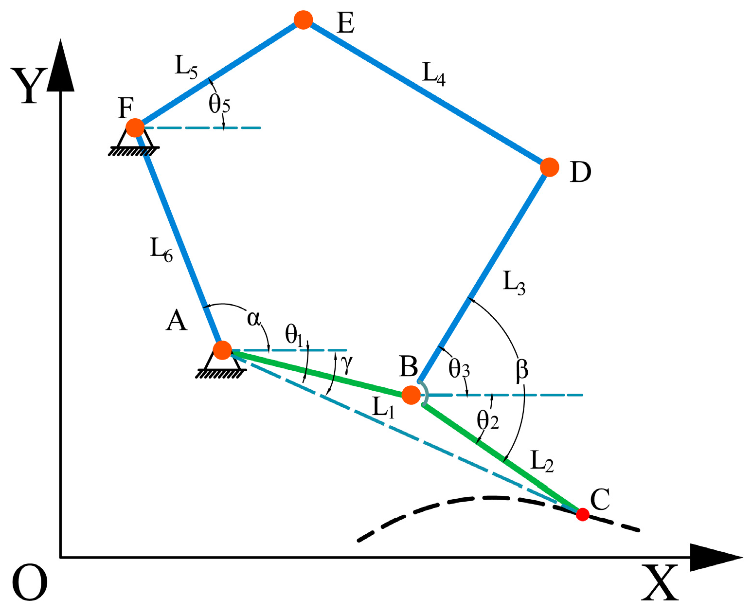
The five-bar mechanism is shown in Figure 2. L1, L2, L3, L4, L5, and L6 represent the lengths of crank AB, linkage BC, linkage BD, linkage DE, crank FE, and frame AF, respectively. Point B is hinged with the linkage AB, point D is hinged with linkage DE, and point C is the end of the mechanism. θ1, θ2, θ3, θ5, α, and γ are the angles between linkage AB, linkage BC, linkage BD, linkage FE, frame AF, connecting line AC, and the positive direction of the x-axis, respectively. β is the angle between linkage BD and linkage BC. xA, yA, xB, yB, xD, yD, xE, yE, xF, and yF are the horizontal and vertical coordinates of frame A, points B, D, and E, and frame F, respectively. The five-bar mechanism is split into two parts. The model consisting of the connecting rod with additional rods and adjacent connecting frame rods is called the trajectory realization model (shown in green), and the rest of the rods and subs are collectively referred to as the compensating motion control model (shown in blue).

2.2.1. Establishment of the Trajectory Realization Model

The track realization model is essentially an open-chain 2R link group [25]. When the target trajectory points are known, the L1 and L2 rod lengths can be determined according to Equations (1)–(3):
L A C = ( y C y A ) 2 + ( x C x A ) 2
L 1 = L A C ( m a x ) L A C ( min ) 2
L 2 = L A C ( m a x ) + L A C ( min ) 2
The ∠BAC and γ can be solved using Equations (4) and (5):
B A C = cos 1 ( L 1 2 + L A C 2 L 2 2 2 L 1 L A C )
γ = a tan 2 ( ( y C y A ) , ( x C x A ) )
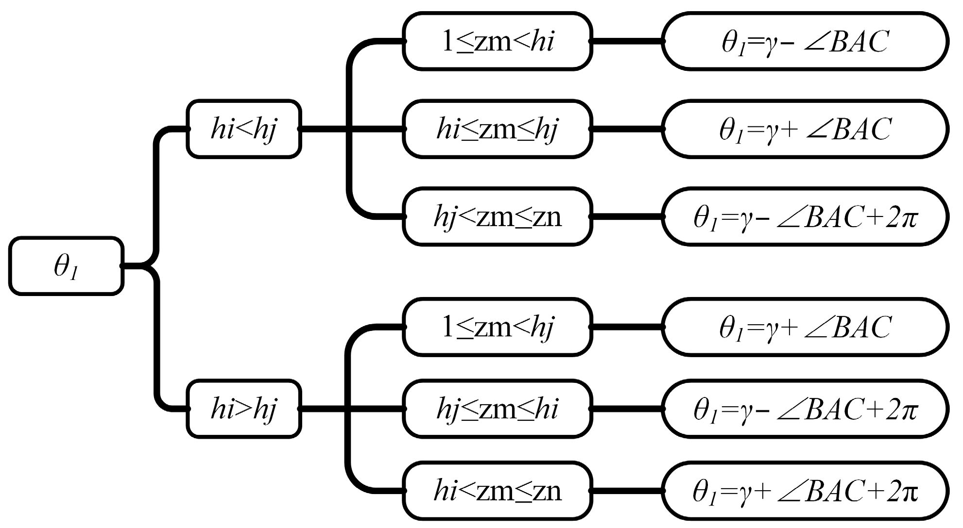
Set the serial number of the trajectory point as zm (zm = 1~zn) and let the hi-th point be the farthest point from the frame A point and the hj-th point be the nearest point to the frame A point. Then, θ1 can be solved according to Figure 3.
The coordinates of point B can be obtained as follows:
{ x B = x A + L 1 cos θ 1 y B = y A + L 1 sin θ 1
And θ2 can be obtained from Equation (7):
θ 2 = a tan 2 ( ( y C y B ) , ( x C x B ) )

2.2.2. Establishment of a Compensation Motion Control Model

Substituting the parameters obtained from the trajectory implementation model into Equation (8), the coordinates of point D can be obtained:
{ x D = x B + L 3 cos ( θ 3 ) = x A + L 1 cos θ 1 + L 3 cos ( β + θ 2 ) y D = y B + L 3 sin ( θ 3 ) = y A + L 1 sin θ 1 + L 3 sin ( β + θ 2 )
Then, the coordinates of point F can be calculated according to Equation (9):
{ x F = x A + L 6 cos ( α ) y F = y A + L 6 sin ( α )
The compensation control model can be seen as solving the problem of open-chain 2R rod FED with a known trajectory point D. According to Equations (10)–(12), the connecting rods L4 and L5 can be obtained:
L F D = ( y D y F ) 2 + ( x D x F ) 2
L 5 = L F D ( m a x ) L F D ( min ) 2
L 4 = L F D ( m a x ) + L F D ( min ) 2
Similarly, using the principles of Equations (4) and (5), and Figure 3, θ5 can be obtained. The mathematical model of the hybrid-drive, five-bar mechanism has been established.

2.3. Establishment of Optimization Model

2.3.1. Establishment of Trajectory Realization Optimization Model

The maximum value of crank rotation angle fluctuation between adjacent track points should be minimized to avoid excessive angular acceleration [26]. The size of the mechanism should be minimized. Therefore, there are two objective functions, which are set as follows:
{ f ( 1 ) = max ( θ 1 m + 1 θ 1 m ) ( m = 1 n 1 ) f ( 2 ) = L 1 + L 2
The coordinates of point A (xA, yA) can be selected as the optimization variable, and its upper and lower limits are set as follows:
{ l o w e r = [ 0 , 0 ] u p p e r = [ 1000 , 1000 ]
The following constraints are considered:
1.
Control the number of motor reversals:
b f ( θ 1 ) + b g ( θ 1 ) 4
where b f ( θ 1 ) and b g ( θ 1 ) , respectively, represent the number of wave peaks and troughs of crank AB’s angular displacement curve.
2.
Avoid interference between the crank and the vegetable turnover box and vegetable packaging conveying device:
y A L 1 > 60
The penalty function method [27] is used for both constraint 1 and constraint 2. Set the optimization model as follows:
{ min [ max ( θ 1 m + 1 θ 1 m ) + M × h 1 ] min [ ( L 1 + L 2 ) + M × h 2 ] }
where h 1 being 0 means constraint 1 is true and h 1 being 1 means constraint 1 is false; h 2 being 0 means constraint 2 is true and h 2 being 1 means constraint 2 is false. M is a larger constant, and an objective function with a larger value will be penalized when the constraint fails.

2.3.2. Establishment of the Compensation Motion Control Optimization Model

Similarly, the objective functions of compensation motion control optimization model are obtained:
{ f ( 1 ) = max ( θ 5 m + 1 θ 5 m ) ( m = 1 n 1 ) f ( 2 ) = L 3 + L 4 + L 5 + L 6
Select the optimization variable as [ L 3 , L 6 , α , β ] , and its upper and lower limits are, respectively, set as follows:
{ l o w e r = [ 0 , 0 , 0 , 0 ] u p p e r = [ 1000 , 1000 , π , π ]
The constraints are as follows:
  • Control the number of motor reversals:
b f ( θ 5 ) + b g ( θ 5 ) 4
where b f ( θ 5 ) and b g ( θ 5 ) , respectively, represent the number of wave peaks and troughs of crank EF’s angular displacement curve.
2.
The five-bar mechanism rod length condition:
{ max [ ( x E x B ) 2 + ( y E y B ) 2 ] < ( L 3 + L 4 ) 2 min [ ( x E x B ) 2 + ( y E y B ) 2 ] > ( L 3 L 4 ) 2
Constraint 1 and constraint 2 also use the penalty function approach, and the final optimization model is:
{ min [ max ( θ 5 m + 1 θ 5 m ) + M × h 1 ] min [ ( L 3 + L 4 + L 5 + L 6 ) + M × h 2 ] }

2.4. Quadratic Optimization of the Pareto Solution Set

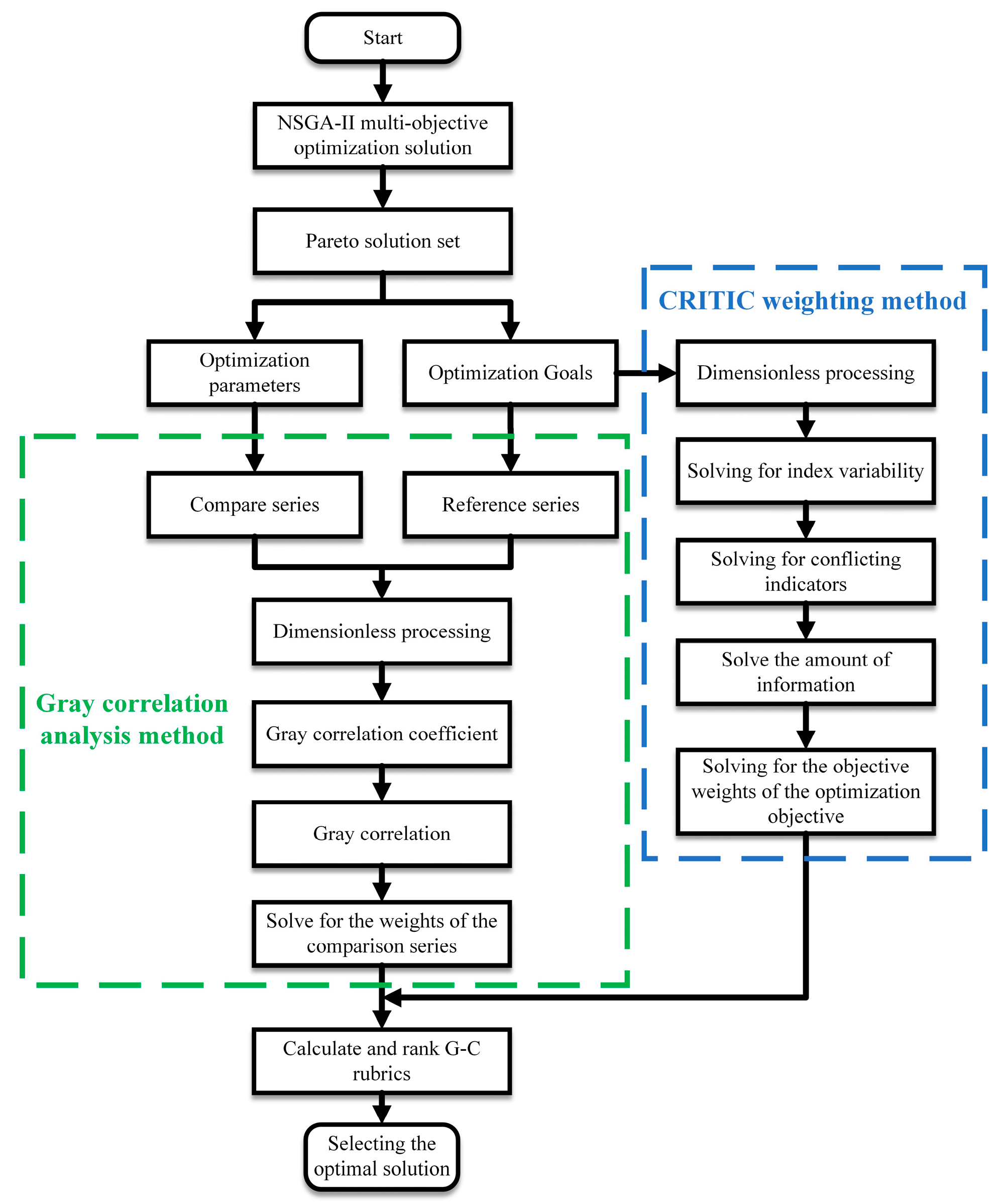
The NSGA-II method introduces an elite strategy to improve the accuracy of the optimization results and uses the crowding distance comparison operator to ensure the diversity of the population [28,29]. However, due to the non-unique number of Pareto frontier solutions ultimately obtained, it is difficult to find the best solution from them. To address this issue, a combination algorithm based on the CRITIC weighting method [30] and grey relational analysis [31] (GRA-C) was proposed for the secondary optimization of the Pareto front solutions. The solution process is illustrated in Figure 4.
First, a set of Pareto solutions are obtained using the NSGA-II multi-objective optimization algorithm. Let the optimization parameters be:
X = [ x 11 x 1 n x m 1 x m n ]
where m is the number of optimization parameters and n is the dimensionality of the optimization parameters.
Let the optimization objective be:
F = [ f 11 f 1 q f p 1 f p q ]
where p is the number of optimization objectives and q is the dimensionality of the optimization objectives.
Second, use Equation (25) to perform dimensionless processing on the optimization objectives and calculate the indicator variability, indicator conflict, and information content according to Equations (26)–(28). Then, use Equation (29) to calculate the objective weight of each optimization objective.
f i j = max ( f i ) f i j max ( f i ) min ( f i ) ( i = 1 ~ p , j = 1 ~ q )
{ f i ¯ = 1 q j = 1 q f i j S i = j = 1 q ( f i j f i ¯ ) 2 q 1
R i = j = 1 q ( 1 r i j )
G i = S i × R i
w i = G i i = 1 p G i
where fi represents the set of solutions of the i-th optimization objective; fij represents the value of the j-th solution of the i-th optimization objective; f i j is the value of the j-th solution of the i-th optimization objective after dimensionless optimization; f i ¯ is the mean value of the i-th optimization objective; S i is the standard deviation of the i-th optimization objective; r i j is the correlation coefficient between evaluation indices i and j; R i is the conflicting nature of the i-th optimization objective; G i is the amount of information contained in the i-th optimization objective; and w i is the objective weight of the i-th optimization objective.
Afterwards, using the optimization goal as the reference sequence and the comparison sequence as the comparative sequence, both were normalized. Equation (30) was then used to calculate the grey correlation coefficient for each comparative sequence with different optimization goals as reference sequences. Equation (31) was further applied to obtain the grey correlation degree of each optimization parameter.
ζ i h ( j ) = min h   min j | f i ( j ) x h ( j ) | + ρ max h   max j | f i ( j ) x h ( j ) | | f i ( j ) x h ( j ) | + ρ max h   max j | f i ( j ) x h ( j ) |
r i h = j = 1 q ζ i h ( j ) q
where f i ( j ) denotes the j-th value of the i-th optimization target; x h ( j ) denotes the j-th value of the h-th optimization parameter; ρ is the discrimination coefficient, which is generally between 0 and 1 and is taken as 0.5; ζ i h ( j ) is the gray relational coefficient of the j-th value of the h-th comparison sequence in the case of the i-th optimization target as the reference series; r i h is the gray correlation of the h-th comparison sequence in the case where the i-th optimization objective is the reference series.
Finally, according to Equation (33), the weight coefficients of each optimization parameter obtained using Equation (32) will be multiplied and added to the normalized optimization parameters of each group. Then, combined with the weight coefficients of the optimization objective obtained using Equation (29), the evaluation index for each Pareto solution can be calculated and referred to as the G-C index. The larger the value of the G-C index, the better the solution is considered. After sorting in descending order based on G-C index, we can obtain the optimal Pareto solutions.
σ i h = r i h h = 1 m r i h
E j = i = 1 p [ w i h = 1 m [ σ i h x h ( j ) ] ]
where σ i h is the weight of the h-th comparison series in the case where the i-th optimization objective is the reference series; E j is the G-C indicator for the j-th set of solutions of the comparison series; and x h ( j ) is the normalized number of the j-th value of the h-th optimization parameter.

3. Results

3.1. Results of the Trajectory Realization Model

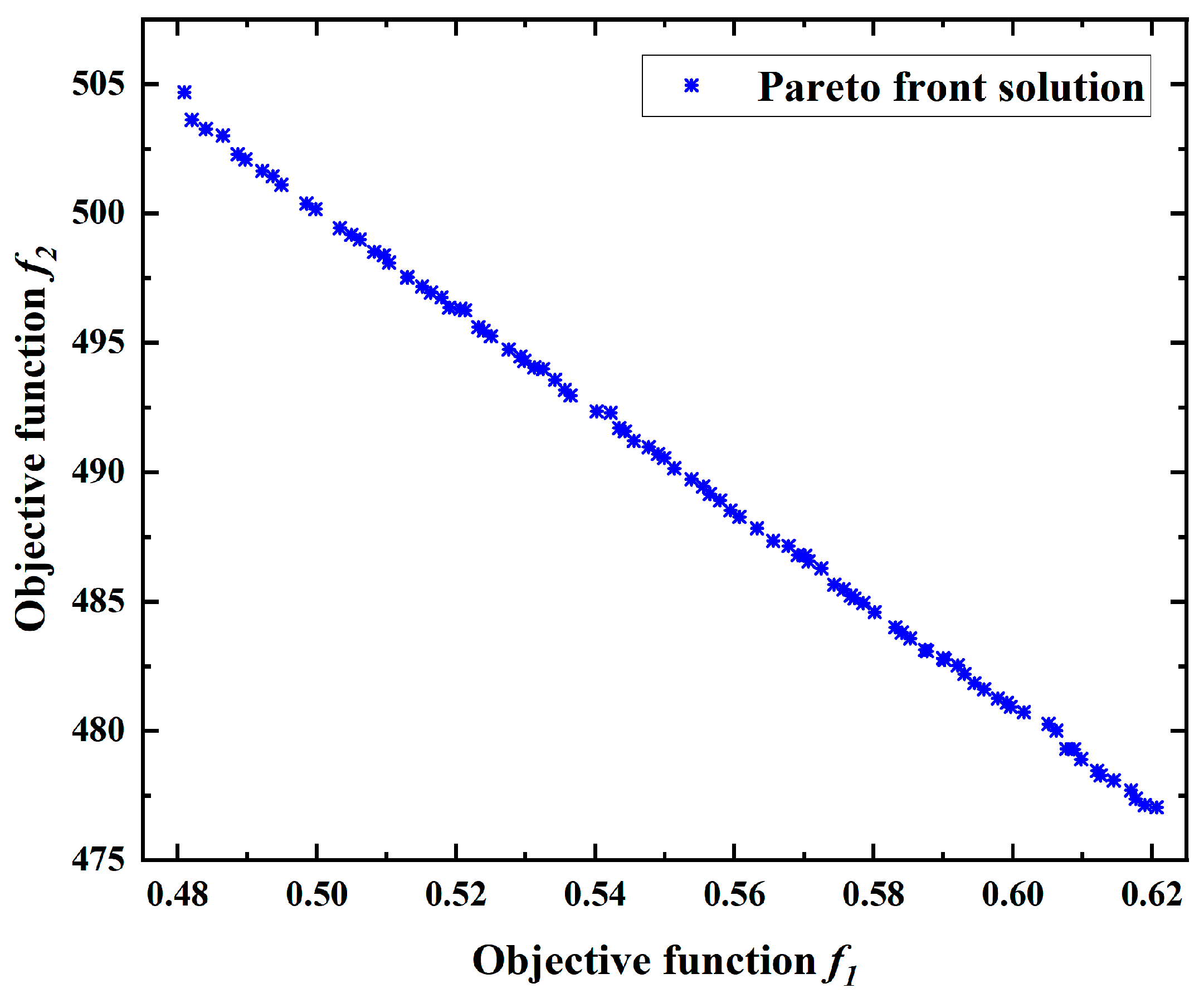
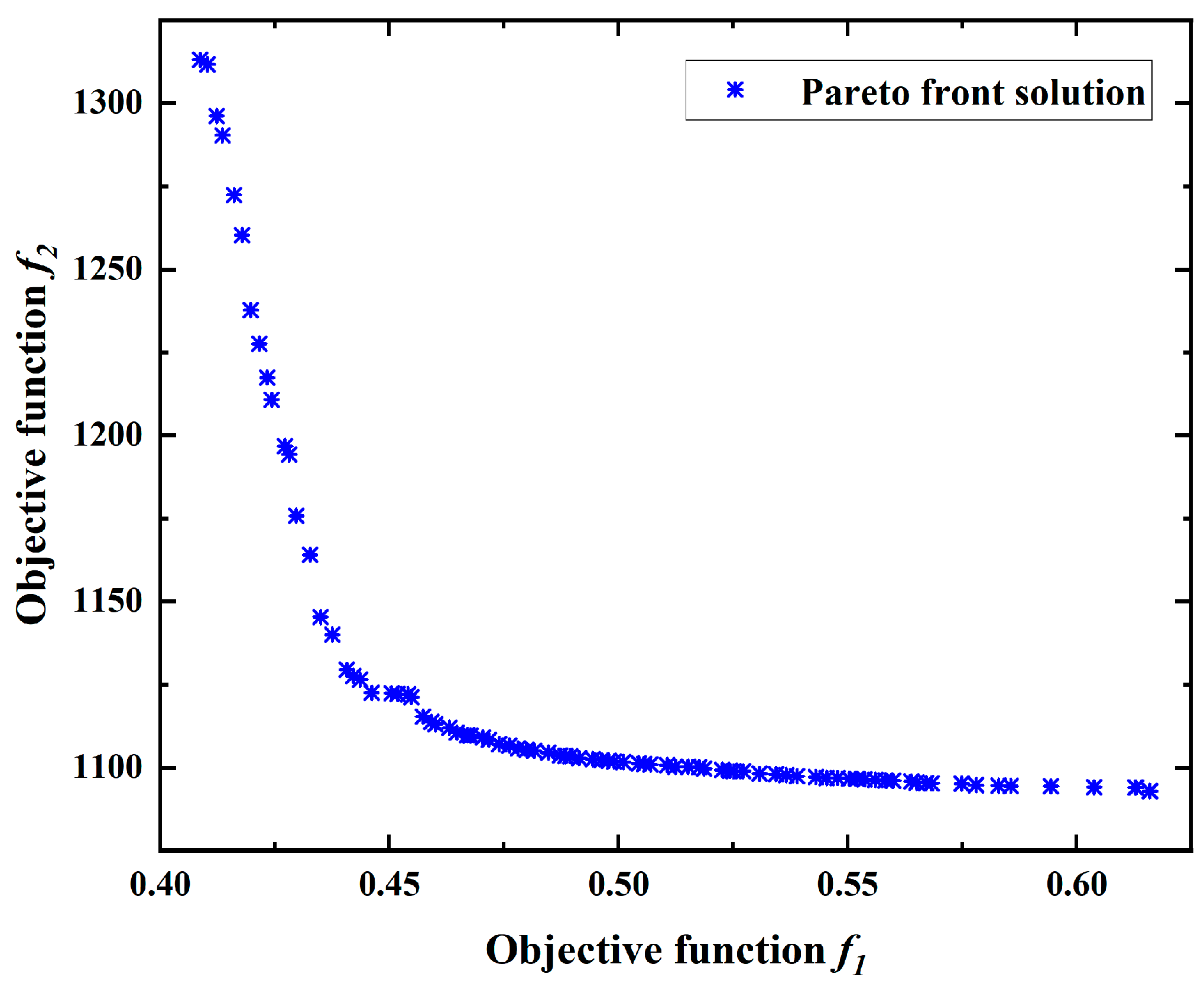
The Pareto front solution shown in Figure 5 is obtained by applying the multi-objective optimization algorithm NSGA-II. Each point in the figure represents a set of solutions which can be taken as the first optimal solution set. The probability of obtaining the optimal solution through manual selection is very low. Therefore, a GRA-C method is proposed to perform quadratic optimization on the Pareto front solution set. The weight of the optimization objective is obtained as shown in Table 3. The G-C index obtained by each Pareto solution is shown in Table 4 (a total of 100 sets of solutions, due to space limitations, the middle part will be omitted), and the best solution obtained using GRA-C is obtained when the Pareto front solution number is 30. The best solution is shown in Table 5.
In order to verify the superiority of the GRA-C method, the genetic algorithm was used to optimize the path realization model of the five-bar mechanism under the same conditions. We set the objective function to 0.5f(1) + 0.5f(2), and used the genetic algorithm to solve this problem. The optimization results obtained are shown in Table 5.
Three Pareto front solutions are selected at the upper left, the diagonal line, and at the lower right of the Pareto front solution diagram in Figure 5. Table 5 provides a comparison between these solutions, the solution obtained by the genetic algorithm, and the solution optimized by the GRA-C, which are, respectively, substituted into the trajectory realization model to obtain the rod lengths L1 and L2.
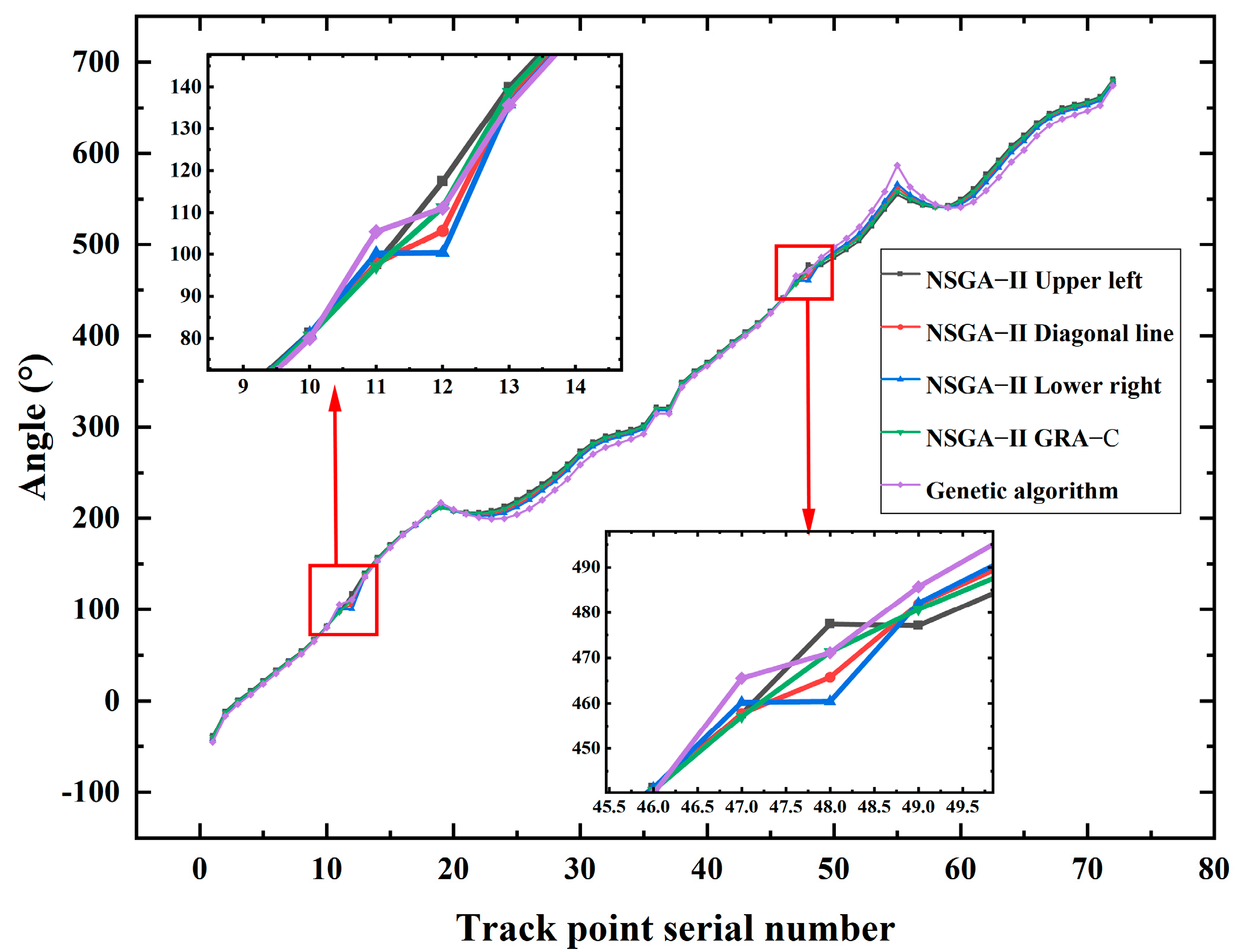
The angular displacement change curves of θ1 and θ2 are shown in Figure 6 and Figure 7. Compared to the four angular displacement curves of NSGA-II, the curve of the genetic algorithm has a peak at the 55th tracking point in Figure 6. This mechanism has an angular acceleration mutation at track points 48–49 on the curve of the upper left solution, and at track points 11–12 and 47–48 on the curve of the lower right solution. The curve of GRA-C is smoother than the other four curves. The curve of the genetic algorithm also has large fluctuations in Figure 7. The mechanism has an angular acceleration mutation at track point 48 on the curve of the upper left solution, at track point 12 on the curve of the diagonal line solution, and at track points 11, 47, and 48 on the curve of the lower right solution.
It can be seen that the solution obtained by GRA-C was superior to the other four sets of solutions. The solution of the GRA-C was used for solving the compensation control model.

3.2. Results of the Compensated Control Model

Similarly, we obtained the Pareto front solution set using the NSGA-II shown in Figure 8 and quadratic optimization solution using the GRA-C. The weight of the optimization objective was obtained as shown in Table 6. The G-C index obtained by each solution of Pareto is shown in Table 7 (a total of 100 sets of solutions, due to space limitations, the middle part will be omitted) and the best solution by GRA-C was obtained when the Pareto front solution number was 13. The best solution is shown in Table 8.
Similarly, the genetic algorithm was used to optimize and solve this part, and the optimization parameters obtained are shown in Table 8.
Table 8 provides a comparison of the five solutions, which are, respectively, substituted into the compensation control model to calculate L4 and L5. The angular displacement curve of the crank L5 is shown in Figure 9. The curve of the diagonal line and the curve of the lower right show obvious fluctuations. The structural dimensions of the mechanism obtained from the solution of the upper left obtained by the NSGA-II and the solution obtained via the genetic algorithm are larger overall.
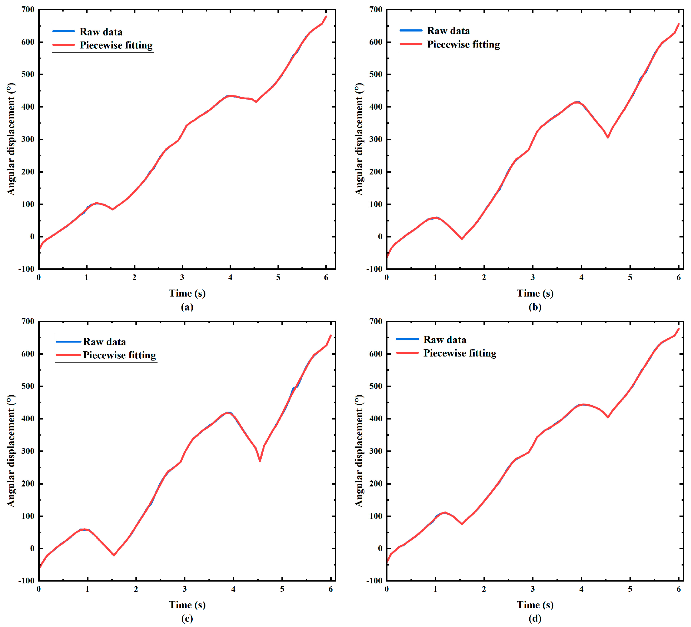
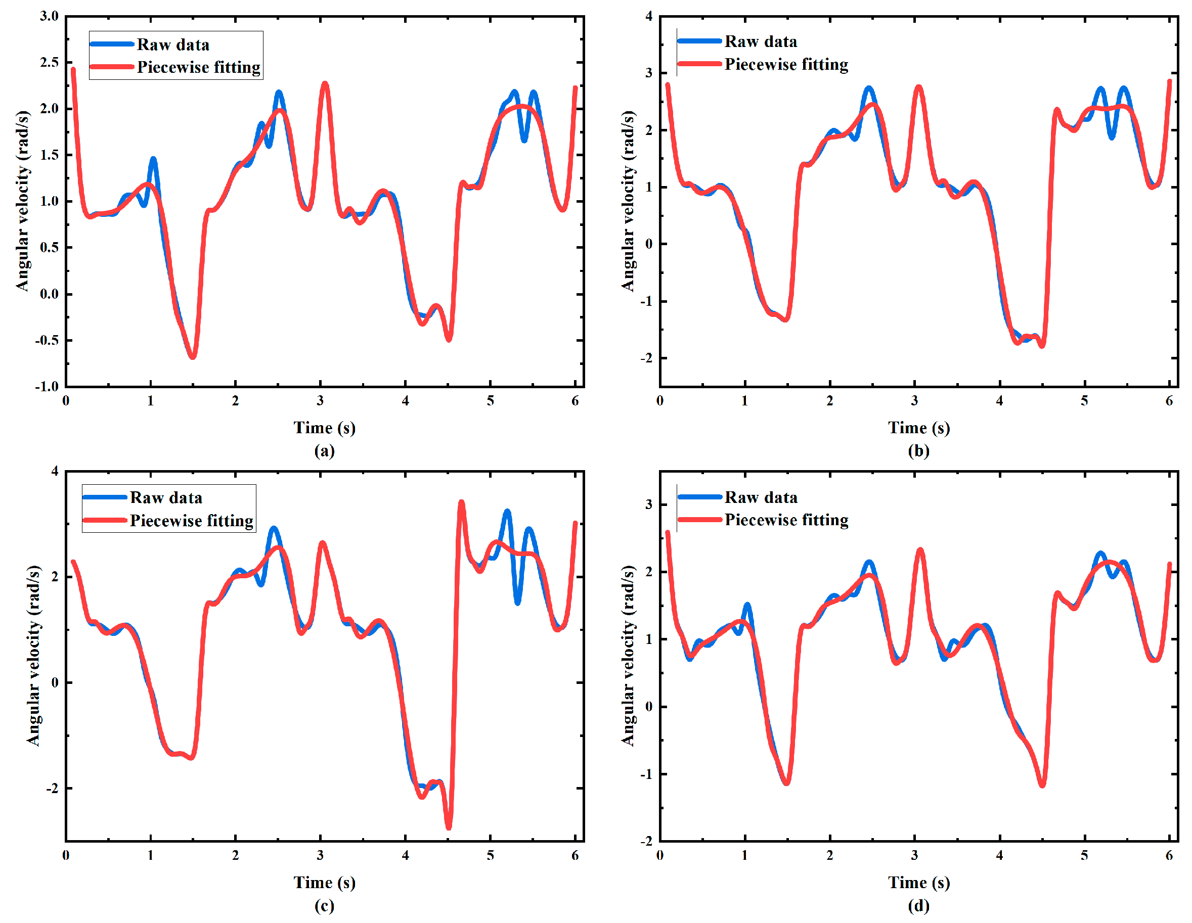
The packing operation requires precise arrival at key trajectory points, while restrictions can be relaxed at secondary trajectory points. In order to reduce the fluctuations in angular velocity and angular acceleration, the angular displacement curve is fitted at secondary trajectory points. The fitted curve is shown in Figure 10.
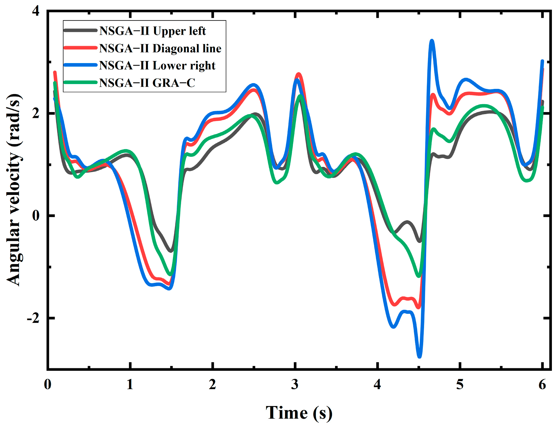
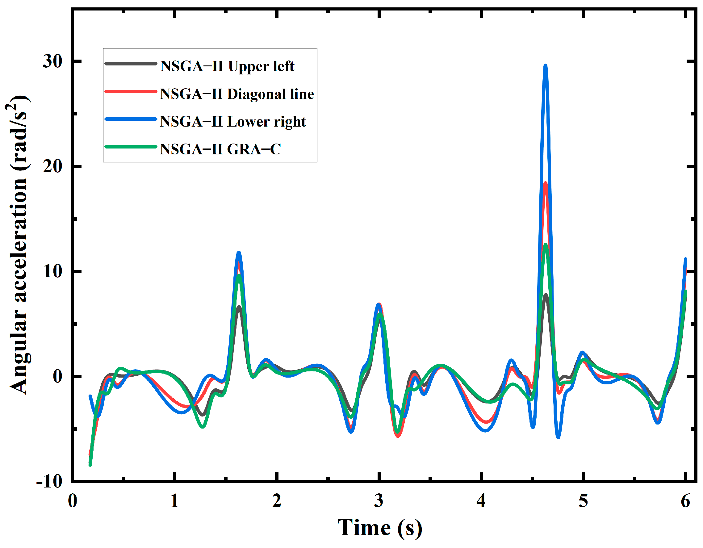
Taking 6 s as a cycle, the angular velocity curve and the angular acceleration curve in a cycle are shown in Figure 11 and Figure 12, respectively, where a is the upper left solution, b is the solution at the diagonal line, c is the lower right solution, and d is the quadratic optimal solution. It can be seen that the fluctuations in the angular velocity and angular acceleration at the secondary trajectory points have decreased.
In Figure 13, the overall fluctuation in the solution of the lower right is the most severe. It can be seen from Table 9 that the peak can reach 3.56 rad/s, the lowest is −2.81 rad/s, and the standard deviation is 1.59. It is obvious that the solution of the diagonal line is not the best. The overall fluctuations in the upper left’s solution and the quadratic optimal solution are relatively small, but the angular velocity of the upper left solution mutates at 4.4 s. We used the standard deviation method to determine the size of the fluctuation in the angular velocity curve for each group of solutions. Comparing the standard deviation of the angular velocity curve obtained by the GRA-C method with the mean of the standard deviation of the other three sets of solutions, it decreased by 26.07%.
Similarly, Figure 14 shows that the angular acceleration curve for the solution in the lower right corner fluctuates considerably, with a peak value of 29.84 rad/s². The curve’s standard deviation is 7.57. The solution in the upper left corner has a mutation in angular acceleration at 4.4 s. Similarly, the standard deviation method is used to calculate the fluctuation in the angular acceleration curve of each group of solutions. Combining Table 8 and Table 10, it can be seen that although the standard deviation of the upper left solution is the smallest among the four sets of solutions, its mechanism size is much larger than that obtained by the GRA-C method. Comparing the standard deviation of the angular acceleration curve obtained by the GRA-C method with the mean value of the standard deviation of the angular acceleration curve of the other three groups of solutions, it decreases by 24.42%.
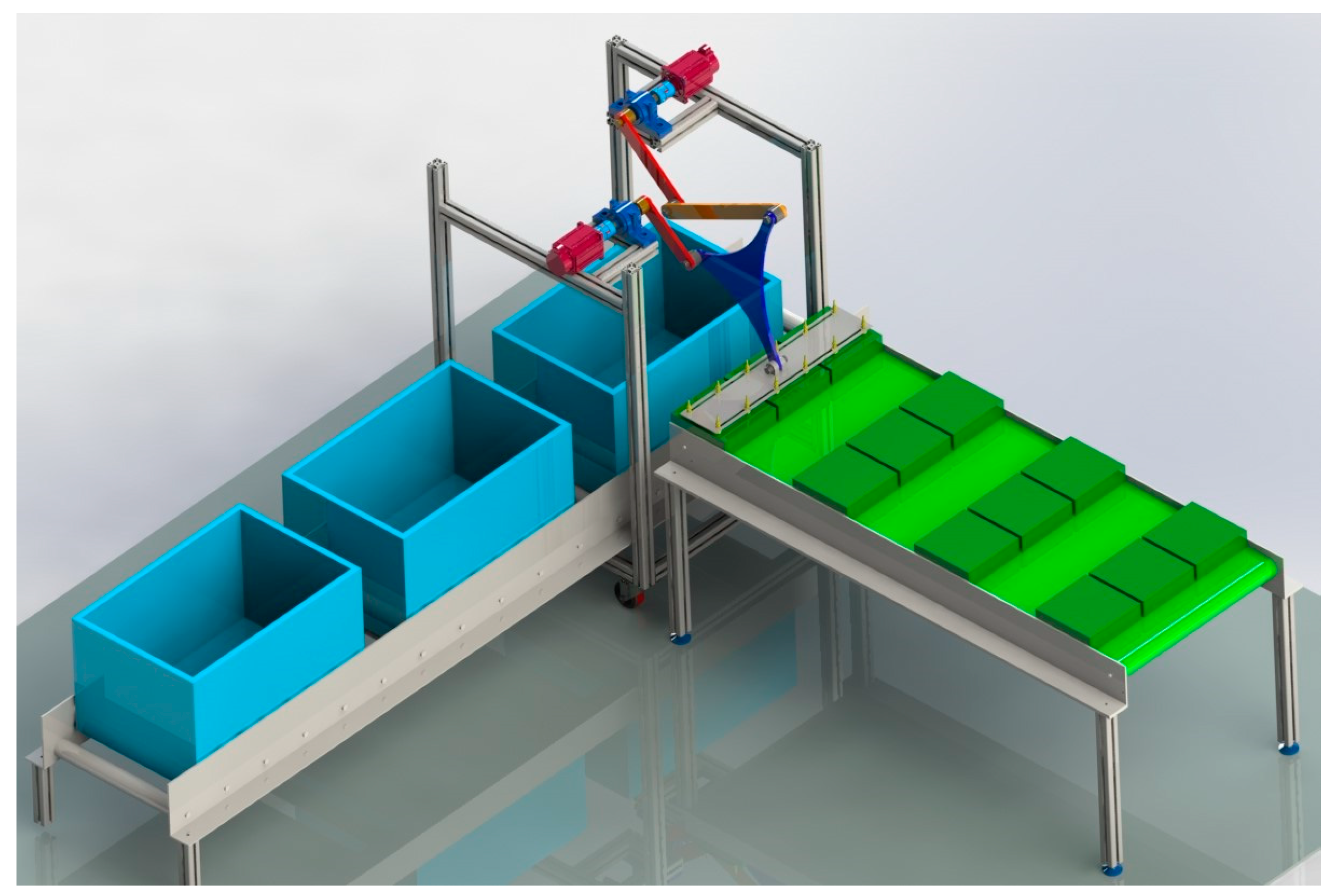
The parameters of the mechanism after quadratic optimization are shown in Table 11. Based on the final optimization parameters, a packaging mechanism for vegetables in an unmanned plant factory was established, as shown in Figure 15.
In order to improve the motion performance of θ1, its angular displacement curve, angular velocity curve, and angular acceleration curve were each fitted piecewise, as shown in Figure 16. The fluctuation in the angular velocity curve and the angular acceleration curve at the secondary trajectory points was greatly reduced.
The angular displacement fitting curves of θ1 and θ5 are each discretized into 720 points (shown in Figure 17) using cubic spline interpolations. As shown in Figure 17, the motion path of the actuator at the end of the mechanism can be obtained by rotating crank L1 and crank L5 according to the motion rules of θ1 and θ5, respectively.
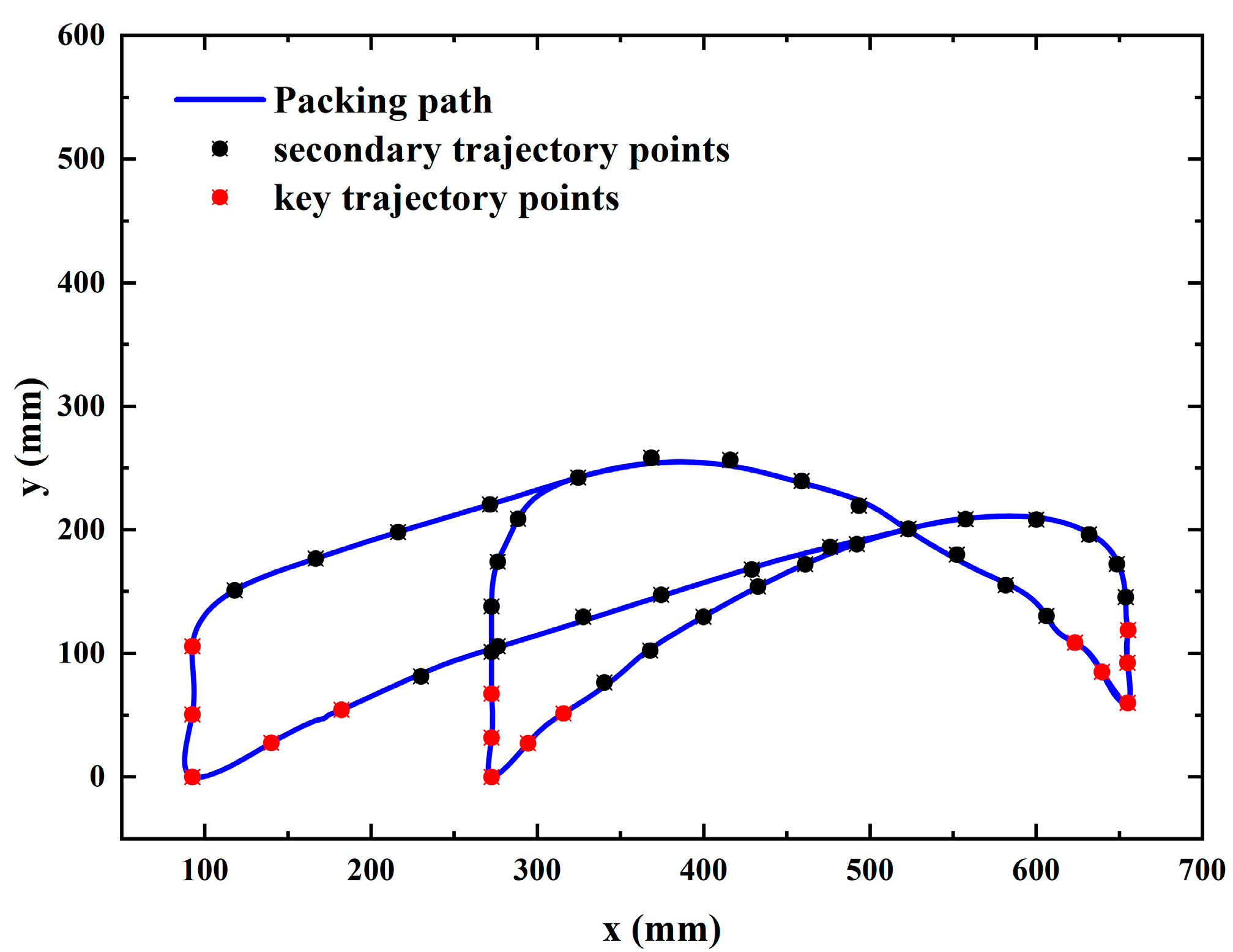
In Figure 18, the red points represent key trajectory points, while the black points indicate secondary trajectory points. The blue curve represents the simulated trajectory. The root mean square deviation between the desired trajectory point and the corresponding simulation trajectory point is calculated as 0.74, and the mechanism can accurately reach the key trajectory point to complete the packing operation of packaged vegetables.
The process of packaging vegetables is shown in Figure 19. First, grab the packaged vegetables at position 19a, move to the box loading position at position 19b, and release the packaged vegetables. Then, return to position 19c, grab the packaged vegetables again, move to the top of another column of the turnover box at position 19d, and release the packaged vegetables. Finally, return to position 19e to start the next cycle.
In mechanism synthesis, the selection of the position and number of key trajectory points not only affects the difficulty and accuracy of the mechanism optimization design but also affects the operational performance of the mechanism. The method of using mixed constraints of key trajectory points and secondary trajectory points can not only improve the accuracy of mechanism operations at critical positions, but it can also provide fuzzy solutions at unimportant positions, improving the selectivity of optimization solutions. Fitting at the secondary trajectory points can improve the kinematic performance of the mechanism to a certain extent. For multi-objective optimization, a good optimization algorithm can not only improve the solution process but can also improve the kinematic performance of the mechanism.

4. Conclusions

  • According to the agronomic requirements of packaging vegetables, the desired trajectory is set, and the trajectory synthesis of the hybrid-drive, five-bar mechanism is completed. On this basis, a hybrid-drive, five-bar vegetable packaging container that can complete fixed-point grasping and release at different points is designed. It can achieve multi-row, multi-column, and multi-layer packaging operations and adapt to the packaging operations in plant factories.
  • The multi-objective optimization NSGA-II algorithm is used to optimize the structural parameters of the five-rod packing vegetable crating mechanism to obtain a set of Pareto front solution sets. A GRA-C method based on a grey correlation analysis and the critic weight method is proposed for the quadratic optimization of the Pareto front solution. A G-C index is designed to judge and obtain the quadratic optimal solution of the Pareto front solution set. The overall size of the optimized rod length obtained using the GRA-C method is 26.71% lower than that obtained using the GA method. Compared with the traditional genetic algorithm, the rod length optimized with the GRA-C method is reduced by 26.71%. The optimal parameters of the five-bar mechanism are as follows: xA = 270 mm, yA = 381 mm, L1 = 176 mm, L2 = 325 mm, L3 = 344 mm, L4 = 417 mm, L5 = 244 mm, L6 = 201 mm, α = 2.58 rad, and β = 1.46 rad. By fitting the four groups of crank angular displacement curves into sections, compared with the average values of the other three groups, the fluctuation in the angular velocity curve decreased by 26.07% and the angular acceleration curve fluctuation decreased by 24.42%.
  • Based on the optimized parameters, the model is established, and its simulation trajectory is obtained. The root mean square error between the simulation trajectory point and the target trajectory point is calculated to be 0.74, which is accurately realized at the critical trajectory points such as the grabbing and releasing of packaged vegetables and basically matches at the secondary trajectory point. The simulation results show that the mechanism can achieve the fixed-point picking and multi-point release of the vegetable packing operation. The feasibility of the combined mathematical model and GRA-C algorithm of the hybrid-drive, five-bar mechanism is verified, and a certain reference value is provided for packing operations in unmanned plants.

Author Contributions

Conceptualization, methodology, data curation, writing—review and editing, validation, and formal analysis, L.Z.; conceptualization, methodology, software, data curation, and writing-original draft, Y.L.; software, data curation, H.Z., Y.J. and L.W.; supervision, project administration, and funding acquisition, J.C. and J.T.; All authors have read and agreed to the published version of the manuscript.

Funding

This research was funded by the National Key Research and Development China Project (2021YFD2000700).

Institutional Review Board Statement

Not applicable.

Data Availability Statement

All data are presented in this article in the form of figures and tables.

Acknowledgments

National Key Research and Development China Project (No. 2021YFD2000700).

Conflicts of Interest

The authors declare no conflict of interest.

References

  1. Toyoki, K. Current Situation and Perspectives of Plant Factory with Artificial Light. Sen-I Gakkaishi 2014, 70, 94–98. [Google Scholar] [CrossRef]
  2. Jin, X.; Zhang, B.; Suo, H.; Lin, C.; Ji, J.; Xie, X. Design and Mechanical Analysis of a Cam-Linked Planetary Gear System Seedling Picking Mechanism. Agriculture 2023, 13, 810. [Google Scholar] [CrossRef]
  3. Hu, S.; Hu, M.; Yan, W.; Zhang, W. Design and Experiment of an Integrated Automatic Transplanting Mechanism for Picking and Planting Pepper Hole Tray Seedlings. Agriculture 2022, 12, 557. [Google Scholar] [CrossRef]
  4. Huang, T.; Li, M.; Li, Z. A 2-DOF Translational Parallel Robot with Revolute Joints. CN Patent 1355087, 31 December 2001. [Google Scholar]
  5. Hu, J.; Yan, X.; Ma, J.; Qi, C.; Francis, K.; Mao, H. Dimensional synthesis and kinematics simulation of a high-speed plug seedling transplanting robot. Comput. Electron. Agric. 2014, 107, 64–72. [Google Scholar] [CrossRef]
  6. Yang, H.; Chen, L.; Ma, Z.; Chen, M.; Zhong, Y.; Deng, F.; Li, M. Computer vision-based high-quality tea automatic plucking robot using Delta parallel manipulator. Comput. Electron. Agric. 2021, 181, 105946. [Google Scholar] [CrossRef]
  7. Li, Y.; Huang, T.; Derek, G.C. An approach for smooth trajectory planning of high-speed pick-and-place parallel robots using quintic B-splines. Mech. Mach. Theory 2018, 126, 479–490. [Google Scholar] [CrossRef] [Green Version]
  8. Li, X. Synthesis of Linkage Mechanisms Based on Fourier Series and Algebraic Method. Ph.D. Thesis, Beijing University of Posts and Telecommunications, Beijing, China. [CrossRef]
  9. Li, X.; Wei, S.; Liao, Q.; Zhang, Y. A novel analytical method for four-bar path generation synthesis based on Fourier series. Mech. Mach. Theory 2020, 144, 103671. [Google Scholar] [CrossRef]
  10. Jacek, B. Use of shape invariants in optimal synthesis of geared five-bar linkage. Mech. Mach. Theory 2010, 45, 273–290. [Google Scholar] [CrossRef]
  11. Mundo, D.; Gatti, G.; Dooner, D. Optimized five-bar linkages with non-circular gears for exact path generation. Mech. Mach. Theory 2009, 44, 751–760. [Google Scholar] [CrossRef]
  12. Modler, K.; Lovasz, E.; Bar, G.; Neumann, R.; Perju, D.; Perner, M.; Margineanu, D. General method for the synthesis of geared linkages with non-circular gears. Mech. Mach. Theory 2009, 44, 726–738. [Google Scholar] [CrossRef]
  13. Yu, C.; Yao, K.; Zong, Y.; Ye, J.; Chen, J. Rigid-Body Guidance Synthesis of Noncircular Gear-Five-Bar Mechanisms and Its Application in a Knee Joint Rehabilitation Device. Machines 2022, 10, 1110. [Google Scholar] [CrossRef]
  14. Zhao, X.; Guo, J.; Li, K.; Dai, L.; Chen, J. Optimal design and experiment of 2-DoF five-bar mechanism for flower seedling transplanting. Comput. Electron. Agric. 2020, 178, 105746. [Google Scholar] [CrossRef]
  15. Zhou, H.; Cheung, E. Analysis and optimal synthesis of hybrid five-bar linkages. Mechatronics 2001, 11, 283–300. [Google Scholar] [CrossRef]
  16. Zhou, H.; Ting, K. Path generation with singularity avoidance for five-bar slider-crank parallel manipulators. Mech. Mach. Theory 2005, 40, 371–384. [Google Scholar] [CrossRef]
  17. Yang, J. Theoretical and Experimental Research on the Trajectory of Controlled Five Bar Mechanisms. Ph. D. Thesis, Wuhan University of Science and Technology, Wuhan, China, 2009. [Google Scholar] [CrossRef]
  18. Acharyya, S.; Mandal, M. Performance of EAs for four-bar linkage synthesis. Mech. Mach. Theory 2009, 44, 1784–1796. [Google Scholar] [CrossRef]
  19. Cabrera, J.; Prado, A. Optimal synthesis of mechanisms with genetic algorithms. Mech. Mach. Theory 2002, 37, 1165–1177. [Google Scholar] [CrossRef] [Green Version]
  20. Penunuri, F.; Peon-Escalante, R.; Villanueva, C.; Pech-Oy, D. Synthesis of mechanisms for single and hybrid tasks using differential evolution. Mech. Mach. Theory 2011, 46, 1335–1349. [Google Scholar] [CrossRef]
  21. Gezgin, E.; Chang, P.; Akhan, A. Synthesis of a Watt II six-bar linkage in the design of a hand rehabilitation robot. Mech. Mach. Theory 2016, 104, 177–189. [Google Scholar] [CrossRef]
  22. Peon-Escalante, R.; Jimenez, F.; Soberanis, M.; Penunuri, F. Path generation with dwells in the optimum dimensional synthesis of Stephenson III six-bar mechanisms. Mech. Mach. Theory 2020, 144, 103650. [Google Scholar] [CrossRef]
  23. Li, J.; Ye, F.; Wang, Z. Dimensional synthesis of a 5-DOF hybrid robot. Mech. Mach. Theory 2020, 150, 103865. [Google Scholar] [CrossRef]
  24. Qu, Z.; Zhang, P.; Hu, Y.; Yang, H.; Guo, T.; Zhang, K.; Zhang, J. Optimal Design of Agricultural Mobile Robot Suspension System Based on NSGA-III and TOPSIS. Agriculture 2023, 13, 207. [Google Scholar] [CrossRef]
  25. Zhao, X.; Wang, C.; Yang, M.; Sun, L.; Cheng, J. Reverse design and analysis of automatic seedling pick-up mechanism with non-circular gear planetary train. Trans. Chin. Soc. Agric. Eng. 2015, 31, 30–36. [Google Scholar] [CrossRef]
  26. Zhao, X.; Cui, H.; Dai, L.; Xu, Y.; Wang, C.; Shen, J. Optimal design and experiment of hybrid-driven five-bar flower potted-seedling transplanting mechanism. Trans. Chin. Soc. Agric. Eng. 2017, 33, 34–40. [Google Scholar] [CrossRef]
  27. Wang, C.; Ma, C.; Zhou, J. A new class of exact penalty functions and penalty algorithms. J. Glob. Optim. 2014, 58, 51–73. [Google Scholar] [CrossRef]
  28. Srinivas, N.; Deb, K. Muiltiobjective Optimization Using Nondominated Sorting in Genetic Algorithms. Evol. Comput. 1994, 2, 221–248. [Google Scholar] [CrossRef]
  29. Deb, K.; Pratap, A.; Agarwal, S.; Meyarivan, T. A fast and elitist multiobjective genetic algorithm: NSGA-II. IEEE Trans. Evol. Comput. 2002, 6, 182–197. [Google Scholar] [CrossRef] [Green Version]
  30. Lu, H.; Zhao, Y.; Zhou, X.; Wei, Z. Selection of Agricultural Machinery Based on Improved CRITIC-Entropy Weight and GRA-TOPSIS Method. Processes 2022, 10, 266. [Google Scholar] [CrossRef]
  31. Tan, Y.; Zhang, Z.; Wang, H.; Zhou, S. Gray Relation Analysis for Optimal Selection of Bridge Reinforcement Scheme Based on Fuzzy-AHP Weights. Math. Probl. Eng. 2021, 2021, 8813940. [Google Scholar] [CrossRef]
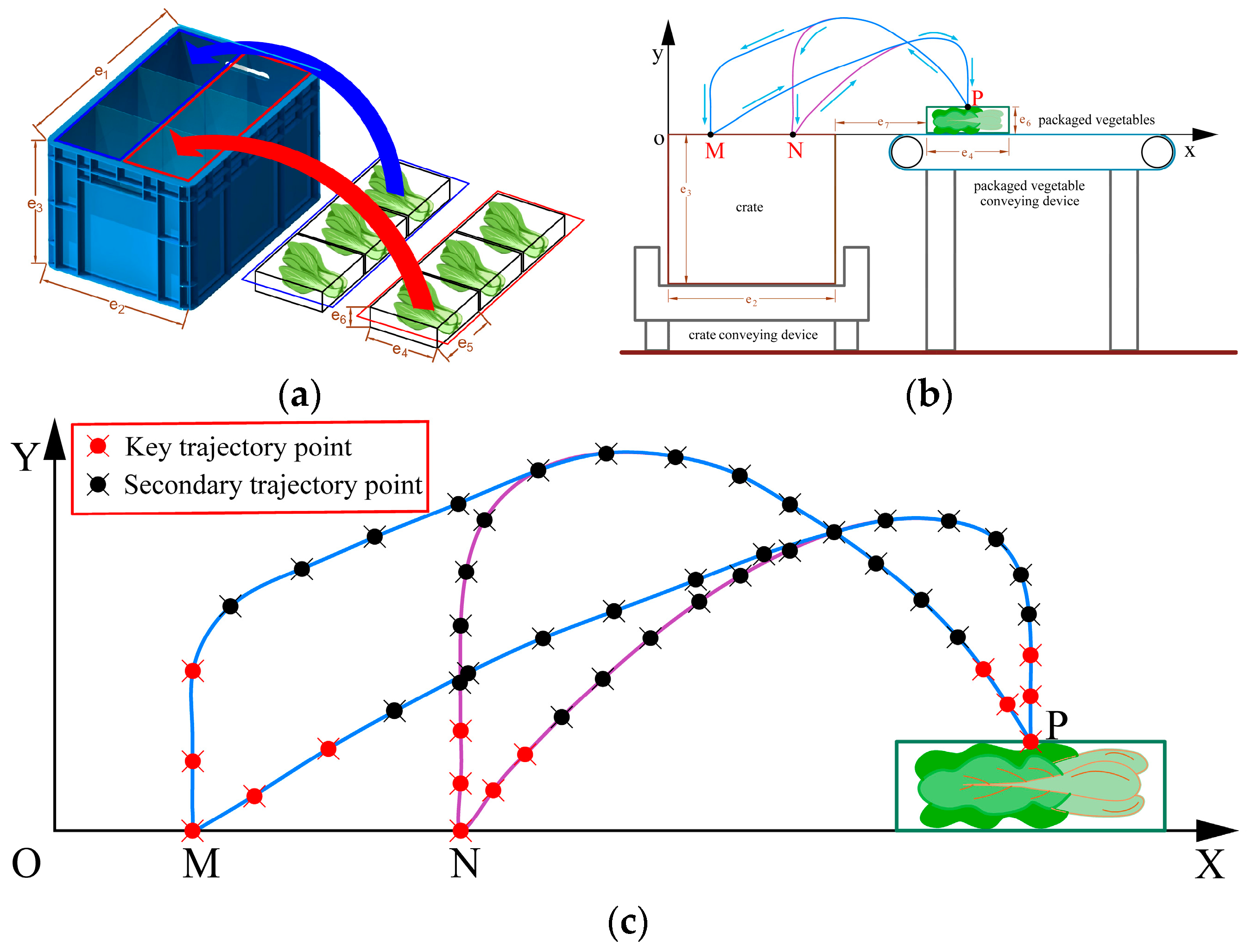
Figure 1. (a) Packing diagram of packaged vegetables; (b) Schematic diagram of packing track; (c) Expected track point.
Agriculture 13 01366 g001
Figure 2. Structure of the five-bar mechanism.
Agriculture 13 01366 g002
Figure 3. Situation of θ1.
Agriculture 13 01366 g003
Figure 4. Flowchart of the GRA-C method.
Agriculture 13 01366 g004
Figure 5. Pareto frontier solution of the trajectory realization model.
Agriculture 13 01366 g005
Figure 6. θ1 angle change curve.
Agriculture 13 01366 g006
Figure 7. θ2 angle change curve.
Agriculture 13 01366 g007
Figure 8. Pareto front solution of the compensated control model.
Agriculture 13 01366 g008
Figure 9. θ5 angle curve.
Agriculture 13 01366 g009
Figure 10. Angular displacement curve after segmented fitting. (a) Upper left; (b) Diagonal line; (c) Lower right; (d) GRA-C.
Agriculture 13 01366 g010
Figure 11. Angular velocity curve after piecewise fitting. (a) Upper left; (b) Diagonal line; (c) Lower right; (d) GRA-C.
Agriculture 13 01366 g011
Figure 12. Angular acceleration curve after piecewise fitting. (a) Upper left; (b) Diagonal line; (c) Lower right; (d) GRA-C.
Agriculture 13 01366 g012
Figure 13. Angular velocity comparison.
Agriculture 13 01366 g013
Figure 14. Comparison of angular acceleration.
Agriculture 13 01366 g014
Figure 15. Vegetable packing machine with a five-bar mechanism.
Agriculture 13 01366 g015
Figure 16. Piecewise fitting curve of a θ1. (a) Angular displacement curve; (b) Angular velocity curve; (c) Angular acceleration curve.
Agriculture 13 01366 g016
Figure 17. (a) Angular displacement interpolation curves of θ1; (b) Angular displacement interpolation curves of θ5.
Agriculture 13 01366 g017
Figure 18. Comparison between target trajectory points and expected trajectory.
Agriculture 13 01366 g018
Figure 19. Packaging simulation of packaged vegetables. (a) During grasping; (b) Packing in the first column; (c) During grasping; (d) Packing in the second column; (e) During grasping.
Agriculture 13 01366 g019
Table 1. Dimensions of turnover boxes and packaged vegetables.
e1 (mm)e2 (mm)e3 (mm)e4 (mm)e5 (mm)e6 (mm)
56536533018018060
Table 2. Expected tracking point values.
Expected Tracking Point Values
No.123456789
xc655.00639.43623.27606.09581.64552.22523.08493.44458.83
yc60.0085.02108.65130.26155.28179.92200.81219.58239.45
No.101112131415161718
xc415.95368.54324.54288.48276.21272.50272.50272.50272.50
yc256.56258.38242.38209.03174.15138.04101.1367.3231.81
No.192021222324252627
xc272.50294.35315.71340.29367.88399.84432.60461.09492.14
yc0.0027.2151.4076.45102.21129.58154.11172.17188.42
No.282930313233343536
xc523.08557.56600.13631.81648.43653.88655.19654.88655.00
yc200.81208.71208.36196.23172.24145.59118.9692.4260.00
No.373839404142434445
xc655.00639.43623.27606.09581.64552.22523.08493.44458.83
yc60.0085.02108.65130.26155.28179.92200.81219.58239.45
No.464748495051525354
xc415.95368.54324.54271.54216.23166.72117.9692.5092.50
yc256.56258.38242.38220.50198.18176.68150.98105.7150.58
No.555657585960616263
xc92.50140.02182.21230.05276.14327.62374.43428.89476.00
yc0.0027.5754.3881.40105.68129.58147.36167.97186.16
No.646566676869707172
xc523.08557.56600.13631.81648.43653.88655.19654.88655.00
yc200.81208.71208.36196.23172.24145.59118.9692.4260.00
Table 3. Weight of f(1) and f(2).
Index VariabilityIndicator ConflictInformation
Content
Weight (%)
Objective function f(1)0.28820.57550.595
Objective function f(2)0.28120.56249.405
Table 4. G-C index of Pareto frontier solution.
Pareto Front Solution NumberG-C Index
1300.5647
2780.5532
3100.5494
4560.5440
5170.5409
6720.5404
7380.5370
8910.5365
9450.5359
10800.5344
………………
100760.4538
Table 5. Parameters obtained from the five sets of solutions.
xA (mm)yA (mm)L1 (mm)L2 (mm)
Upper left250.5628384.7431179.1226339.5562
Diagonal line285.3488381.2346172.724317.0068
Lower right299.5354378.1534169.4951307.5559
GRA-C270.2977381.3713176.0371325.2341
Genetic algorithm331.374388.5577160.7161300.4606
Table 6. Weights of f(1) and f(2).
Index VariabilityIndicator ConflictInformation ContentWeight (%)
Optimization objective f(1)0.1121.7420.19566.987
Optimization objective f(2)0.0551.7420.09633.013
Table 7. G-C indicators of the Pareto front solution.
Pareto Front Solution NumberG-C Index
1130.7495
2280.5920
3680.5871
4570.4888
5150.4800
6780.4768
7810.4035
8510.4011
9730.3841
10760.3770
100640.1724
Table 8. Parameters of the five-bar mechanism corresponding to the five sets of solutions.
L3 (mm)L4 (mm)L5 (mm)L6 (mm)α (rad)β (rad)
Upper left396.3049524.0375326.2744433.47382.79632.0138
Diagonal line435.1599537.5038190.4173279.77171.54540.6466
Lower right417.2988486.2555170.4382239.94481.31570.5280
GRA-C343.7272416.7531244.2831200.09902.58421.4603
Genetic algorithm470.1084615.9876255.3532302.44282.41961.1934
Table 9. Angular velocity curve data.
Lowest (rad/s)Highest (rad/s)Standard Deviation (rad/s)
Upper left−0.742.460.76
Diagonal line−1.892.861.34
Lower right−2.813.561.59
GRA-C−1.122.520.91
Table 10. Angular acceleration curve data.
Lowest (rad/s2)Highest (rad/s2)Standard Deviation (rad/s2)
Upper left−8.147.893.1
Diagonal line−7.7318.225.08
Lower right−6.8929.847.57
GRA-C−8.2112.523.95
Table 11. Optimal parameters of the controlled five-bar mechanism.
xA
(mm)
yA
(mm)
L1
(mm)
L2
(mm)
L3
(mm)
L4
(mm)
L5
(mm)
L6
(mm)
α
(rad)
β
(rad)
Optimal solution2703811763253444172442012.581.46
Disclaimer/Publisher’s Note: The statements, opinions and data contained in all publications are solely those of the individual author(s) and contributor(s) and not of MDPI and/or the editor(s). MDPI and/or the editor(s) disclaim responsibility for any injury to people or property resulting from any ideas, methods, instructions or products referred to in the content.