A Hybrid Framework for Detection and Analysis of Leaf Blight Using Guava Leaves Imaging

Abstract

Fruit is an essential element of human life and a significant gain for the agriculture sector. Guava is a common fruit found in different countries. It is considered the fourth primary fruit in Pakistan. Several bacterial and fungal diseases found in guava fruit decrease production daily. Leaf Blight is a common disease found in guava fruit that affects the growth and production of fruit. Automatic detection of leaf blight disease in guava fruit can help avoid decreases in its production. In this research, we proposed a CNN-based deep model named SidNet. The proposed model contains thirty-three layers. We used a guava dataset for early recognition of leaf blight, which consists of two classes. Initially, the YCbCr color space was employed as a preprocessing step in detecting leaf blight. As the original dataset was small, data augmentation was performed. DarkNet-53, AlexNet, and the proposed SidNet were used for feature acquisition. The features were fused to get the best-desired results. Binary Gray Wolf Optimization (BGWO) was used on the fused features for feature selection. The optimized features were given to the variants of SVM and KNN classifiers for classification. The experiments were performed on 5- and 10-fold cross validation. The highest achievable outcomes were 98.9% with 5-fold and 99.2% with 10-fold cross validation, confirming the evidence that the identification of Leaf Blight is accurate, successful, and efficient.

1. Introduction

Food is the fundamental requirement for the existence of human beings, and it is the notable outcome of agricultural activities. Agriculture is assumed to be the backbone of economic development, as it exhibits the cultivation of multiple crops, fruits, and vegetables. There is a large difference between the cultivation and annual production of fruits because of inappropriate advancements in technology, lack of knowledge, and diseases that negatively affect the production [1]. Disease detection in plants is a challenging task and is essential to diagnose at early stages. Diseases are mostly diagnosed through leaves because they tend to highlight contaminated parts immediately. Guava is an important fruit in agriculture; therefore, its leaves are selected for the detection and recognition of diseases [2]. Guava is nutritionally beneficial, serving calcium and iron to the human body. It is cultivated in America, especially in Mexico, Thailand, South Africa, and many other countries. Many laboratories such as the Central Institute of Subtropical Horticulture (CISH) and different institutes are continuing to work on guava production in different areas of the world [3]. Several diseases, such as bacterial and fungal diseases, attack the guava fruit, which badly affects its production [4]. There are different techniques of ML applied for disease detection. Almost 177 types of diseases are found that damage leaves, causing leaf blight and leaf spots. Known diseases include brown roots, twig drying, bacterial wilt, anthracnose, ring rots, and many others [5].

Many researchers aim for innovations in disease detection. Disease detection relies on five major steps. Usually, the first step in image processing is image acquisition. After obtaining images, preprocessing incorporates multiple steps that result in better accuracy. After preprocessing, feature extraction is performed, where the features of the images are boosted for further computation and selection. The final stage is classification. A variety of models are presented using diverse methodologies such as convolution neural network (CNN), gradient descent (GD), and many others for classification purposes [6]. Convolution neural networks play an essential part in the extraction of features through hidden layers, as manual extraction is costly and time-consuming [7]. Plant pathologists need an automatic detection system to diagnose leaf blight in plants.

The main focus of the proposed methodology is the detection and classification of leaf blight. Leaf blight affects plants as a result of a pathogenic organism infecting leaves. Therefore, an automated system is needed to detect leaf blight disease. Research of diseases in guava fruit is a challenging task, as it seeks a variety of data regarding diseases in the relevant field [8]. The forecasted production of guava is 498.95 thousand tonnes in 61.37 acres in the year 2020–2021 and the production of guava is 499.68 thousand tonnes in 61.37 acres in the year 2021–2022. Evaluation of the researched tasks becomes critical with time due to the wide range of diseases, and a great deal of effort has already been applied towards the relevant field [9].

There are several limits and difficulties in detecting and classifying guava plant diseases in the existing literature. Some major problems per the literature are the poor contrast, variation in shape, texture, and size, and illumination problems found in disease images that make them difficult to recognize and classify.

This article presents a new methodology for the detection of leaf blight. The purpose is to classify the healthy and diseased images of guava leaves with improved accuracy. The significant contributions presented in this research are as follows:

• A new deep CNN Net named SidNet is presented, which consists of 33 layers along with 35 connections. The pretraining of SidNet is performed on a plant imaging dataset. The features are extracted from the proposed SidNet, darknet53, and AlexNet, which are further fused using serial fusion. The deep features are also known as automatic features; they automatically solve the issues related to contrast, shape, texture, and illumination.
• The features are sorted using an Entropy Algorithm, and for better feature selection, Binary Gray Wolf Optimization is used. The selected features are used to make a single feature vector for classification using an SVM and KNN Classifier to achieve the best performance and results.
• Data Augmentation is performed, as the selected dataset is small; therefore, the images are flipped both horizontally and vertically to make the dataset large.

The paper consists of five sections, where Section 1 explains the introduction, motivation, contribution, and problem statements for leaf blight detection. Section 2 covers the recent existing work. Section 3 provides the details of the presented proposed framework and Section 4 describes the details of the experiments and outcomes. Lastly, Section 5 covers the conclusion.

2. Related Work

Diseases in fruit plants and leaves are a major cause of destruction and economic loss. Automated systems help greatly with the detection of diseases at early stages. While considering the field of detection of disease in plants, deep neural networks work perfectly to identify and classify diseases. These networks are mentored to conduct high-value results in detecting and classifying diseases, and to fulfill the demands of food deformation prevention.

There are different methods for collecting images under certain conditions. Images are captured by multiple appliances, such as cameras, sensors, mobile phones, and other devices. In this era, more datasets containing guava are publicly available on multiple forums, such as Kaggle, Mendeley, and many others [10]. Pre-processing of images is an important phase in image processing. The pre-processing phase entails multiple steps which help highlight the focused parts and remove irrelevant information from guava leaf images. In the real world, label noise on images is a matter of concern. Multiple techniques have attained the best results in denoising images, especially mixed noise, speckle noise, and salt and pepper noise. Low contrast and color distortion in guava leaf images make them blur. Scattering and light absorption also affect clear image visualization [11]. Images are preprocessed by using rotational filters such as horizontal and vertical flipping. Data augmentation techniques are used, such as applying rotations and zooming into images [12]. Color spacing techniques are extensively applied in image processing. RGB, CIELAB, and CMYK models are mostly used as color spacing techniques to give the best results.

Feature extraction is a process in which reatures are reduced from the raw dataset and new features for manageable processing are created. Texture analysis has a wide range of applications [13]. Pattern recognition requires feature extraction to solve problems in prediction, cluster discrimination, and representation of data in the best way [14,15]. Content-Based Image Retrieval (CBIR) converts high-level image visuals into feature vectors that contain some properties [16]. There are multiple techniques to extract the features from guava leaf images, such as handcrafted-based features, region-based features, deep CNN-based features, texture-based features, color-based features, morphological-based features, etc. Extraction of features is categorized into hand-crafted-based features and deep-based features.

The selection of features from plant leaf images is carried out after the extraction of hand engineered and deep-based features. The set of features is chosen while noisy, poor, and extra features are eliminated from the original set of features [17]. There are five main types of feature selection, which are (1) Linear Method, (2) Non-Linear Method, (3) Filter-Based Method, (4) Wrapper Method, (5) Embedded Method. Linear methods include PCA and LDA. PCA stands for Principal Component Analysis, which is used for data reduction [18]. LDA stands for Linear Discriminant Analysis and is used for the conversion of high dimension features into lower dimension features [19]. Non-linear methods include Entropy [20], Genetic Algorithm (GA) [21], Binary Gray Wolf [22], Slap Swarm [23], Atom Search [24] and many others. Filter methods includes mRMR [25], Missing Value Ratio [26], and many others. Wrapper methods include Jackstraw [27] and Boruta [28]. Finally, embedded methods include LASSO [29], Ridge [30], Elastic [31], and many others. Image fusion [32] helps greatly in improving classifier accuracy with less computational cost [33]. Different algorithms are proposed that use image fusion to get the best accuracy results.

Image classification is the last step in image processing [34]. Classification tends to dominate the feature vector to determine which object belongs to which class [35]. There are different types of techniques used for the classification of healthy and diseased images of plant leaves. Image classification is divided into three main categories, which are (1) Supervised Learning, (2) Unsupervised learning, and (3) Object-based image analysis. Supervised Learning is used to detect the new category of the object from training data [36]. Unsupervised Learning is a process in which an image is identified in an image collection without using labeled training data [37]. Object-based analysis involves the grouping of pixels on the basis of some similarities such as shape and neighborhood [38]. To get the most accurate results, the Plant Village dataset is used for testing and training purposes. A total of 80% of guava leaf images are used for testing while 20% of them are used for training purposes. The achievable accuracy is 97.22% using Alex-Net and Squeeze-Net after segmentation and classification [39]. Atila et al. [40] designed the Efficient-Net architecture, which is designed for classification purposes. Different architectures are applied using CNN for model training to get highly accurate results. The model training is performed on the dataset of 87,848 images. Images are preprocessed using different techniques such as downscaling and squaring methods, they are then classified, and an accuracy of 99.53% is achieved using AlexNet, VGG-16, and GoogLeNet [41]. Several algorithms are used for image classification. These are SVM [42], K-Nearest Neighbor (KNN) [43], Naïve Bayes [44], Shadow algorithms [45], Minimum Mean Distance (MMD) [46], Decision Trees [47], K-Means Clustering [48] and many others. The datasets are frequently classified by SVM. This involves supervised learning and comprises points that are in the sample space and different regions [49]. Segmentation is performed on the preprocessed data in three stages. In the first stage, the deep CNN is trained to learn the mapping from the space map. In the second stage, prediction-based labels are acquired. At the last stage, these acquired labeled images are sent to SVM for classification and achieve an accuracy of 86% [50]. In machine learning, KNN is a statistical classification algorithm. It gathers the objects selected by neighbors having the highest number of votes [51]. KNN is inspected for the detection of weeds from UAV images of the chili crop of Australia. In comparison with KNN, SVM and Random Forest (RF) are used. The achievable accuracies across RF, SVM, and KNN are 96%, 94%, and 63%, respectively [52]. KNN is also used for classifying facial expressions [53]. Additionally, KNN is used for the classification of grape leaves into healthy and unhealthy leaves. Texture-based and color-based features are extracted from grape leaf images and are classified by the KNN classifier, and an accuracy of 96.66% is achieved [54]. Table 1 depicts an overview of recent works related to plants diseases analysis

Table 1. An overview of recent literature regarding plants diseases analysis.

Ref.	Year	Techniques	Dataset	Diseases	Results %
[41]	2018	Downscaling and squaring method, AlexNet, VGG-16, AlexNetOWTBn.	87,848 58 classes	Apple Scab, Black Rot, Early Blight, Brown Leaf Spot	99.53
[55]	2018	ResNet-50, Deep Siamese convolutional network, TSNE method, KNN	PVD	Black Rot, Esca, Chlorosis	90
[56]	2018	Transfer learning, F-RCNN, classification.	4923	Phoma Rot, Leaf Miner, Target Spot	95.75
[57]	2019	F-CNN, S-CNN, Segmentation, annotation and labeling on region of interest (lesions), random transformation (stretch/rotation/brightness/contrast blur)	Independent dataset	Spider Mite, Target Spot	98.6
[58]	2019	VGG classification, resizing and transformation of images into grayscale,	2465	Black dot and scurf	96
[40]	2021	Efficient-Net (B5Ver), Alexnet, ResNet50, classification.	61,486	Late Blight, Bacterial Spot	99.97
[59]	2021	Resizing, normalizing and augmentation, Efficient-Net (B7Ver), Efficient-Net (B4Ver), U-net, and modified U-net segmentation model, Score-Cam visualization technique,	18,161	Target Spot	99.9

3. Materials and Methods

The proposed methodology consists of multiple phases of image processing. In the first step, as a preprocessing step, color spacing is performed on the images of the dataset. Images are converted from RGB color format to YCbCr color format. After getting preprocessed data, feature extraction is performed using two pretrained models and a newly proposed CNN deep model known as SidNet. This newly proposed model is based on 33 convolutional layers. This proposed CNN deep model is pretrained using the Plant-Village dataset, which consists of 38 classes. After pretraining, features are collected from the proposed CNN deep model. These extracted features are then fused with AlexNet and DarkNet-53 to find the best and most appropriate results. A deep CNN known as AlexNet was developed in 2012, which is an 8-layer deep model and consists of 5 convolution layers and 3 Fully Connected layers. After every convolution layer and fully connected layer, ReLU is applied. It contains a dropout layer, which is applied after the first and second fully connected layer. The input size in AlexNet is 227 × 227. In all layers, the activation function is ReLU. Softmax is designed as an activation function in the output layer. AlexNet is the simplest deep CNN model and it is used to get highly accurate results. DarkNet-53 is another used deep model, which works as the backbone for YoloV3 in object detection. It contains 25 layers for batch normalization and Leaky ReLU. The input size is 256 × 256 in DarkNet-53. In the second step, the feature sorting entropy algorithm is used for the selection of the best features. These selected core features are fused using serial-based fusion. After fusing the core features, the binary gray wolf optimization algorithm is used. Finally, these extracted fused features are provided to SVM and KNN classifiers for the classification of Leaf Blight for the best achievable results. The complete view of the proposed model is shown in Figure 1. It covers a complete view of the flow of the diagram of the designed structure.

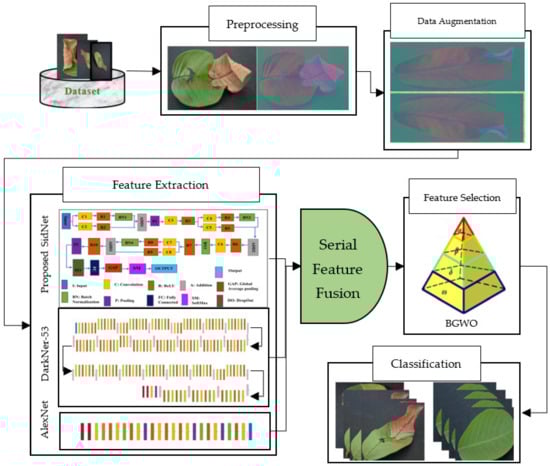
Figure 1. Proposed Framework for disease recognition in guava leaves.

3.1. Image Preprocessing

In image processing, color space conversion is an important task. RGB is used to store real-time images and videos because it allows for the sensitivity of color detection cells for the human visual system. YCbCr is beneficial for its low-resolution capability for the human visual system. Therefore, the conversion of RGB to YCbCr is mostly used in image processing. The general formula is given below:

$$\mathit{YCbCr}= \mathit{RGB} 2\mathit{YCbCr} \left(\mathit{RGB}\right)$$

(1)

This is the general formula that is used for the conversion of RGB to YCbCr and it represents 8 bits per sample pixel in RGB format. The white and black colors are represented on a scale from 0 to 255. Therefore, the components of YCbCr are obtained from the following equations.

$$Y=16+65.738/256 R+129.057/256 G+25.064/256 B$$

(2)

$$Cb=128+37.945/256 R-74.494/256 G+112.439/256 B$$

(3)

$$Cr=128+112.439/256 R-94.154/256 G+18.285/256 B$$

(4)

where $Y$ is used to represent the luma (luminance) component. $Cb$ represents chrominance blue and $Cr$ represents chrominance red. These numbers are the constant values that are used to adjust the value of Y. Figure 2 shows the conversion from RGB to Y$CbCr$.

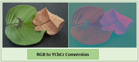
Figure 2. RGB to YCbCr conversion.

3.2. Data Augmentation

For data augmentation, horizontal and vertical flipping are used. According to the mathematical model, the horizontal flipping of the images is presented as follows:

$$H_F \left(-x, y\right)=H_O \left(x, y\right)$$

(5)

And the vertical flipping of the images is presented as follows:

$$H_V \left(x,-y\right)=H_O\left(x, y\right)$$

(6)

H_F shows the flipping function and H_O shows the original image function that is to be flipped. H_v shows the flipping function and H_O shows the original image function that is to be flipped.

3.3. Feature Extraction

After preprocessing and augmentation, the next phase is feature extraction. In this phase, with the help of pretrained models, the most optimal features are extracted. According to our proposed methodology, a newly designed model named SidNet, and other pretrained models such as DarkNet-53 and AlexNet, are used for extracting the most optimal features.

3.4. Proposed SidNet as CNN Net

This proposed CNN Net is a blockbuster CNN-based architecture used for the detection and classification of Leaf Blight. The proposed SidNet model consists of 33 layers involving 8 convolutional layers, 10 ReLU layers, 4 layers of batch normalization, one dropout layer, one softmax layer, one classification output, one fully connected, and one global average pooling layer. The Input size of the Proposed CNN Net is “227 × 227 × 3” and it contains 35 connections. The stride is “1 × 1” throughout the proposed framework’s convolution layer. The number of filters is set to 96 in all convolutional layers of the framework, while the padding dimensions vary according to the convolution layer used in the different stages of architecture. The padding of the last convolution layer is 5, 5, 5, 5. Two pooling layers are used, where the stride for the two pooling layers in the architecture is “2 × 2”. While the pooling size of the first pooling layer is 3, 2 and the pooling size of the second pooling layer is 3, 3. The mean decay and variance decay for all batch normalization layers are 0.1. Figure 3 shows the architecture of the proposed SidNet.

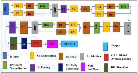
Figure 3. The architecture of the proposed CNN network, SidNet.

The proposed deep model named SidNet comprises 33 convolution layers. Its Input size is “227 × 227 × 3” and it contains 35 connections.

Due to the small number of samples of the available dataset, the proposed deep model with softmax (SM) classifier is first trained on the third-party dataset named CIFAR 100 [60]. Then, the guava leaf dataset is fed to SidNet for feature extraction. The features are extracted from the fully connected (FC) layer. These features, after feature selection, are trained and tested on various classifiers (such as SVM with its variants and KNN with its variants) for evaluation. According to our model, the features in SidNet are presented as:

$$f_{e\times f}=\{ L1\times 1 , L1\times 2 , L1\times 3 , \dots \dots \dots ..L1\times \mathrm{p} \}$$

(7)

where L (1_…p) represents the number of features obtained from the proposed CNN model, which is known as SidNet, and e × f is the dimension of the resultant function.

Visualization of the strongest feature maps at different convolution layers with the proposed SidNet architecture is shown in Figure 4. The visualization is performed on conv_1, conv_2, conv_3, conv_4, conv_5, conv_6, conv_7, and conv2 of the proposed architecture.

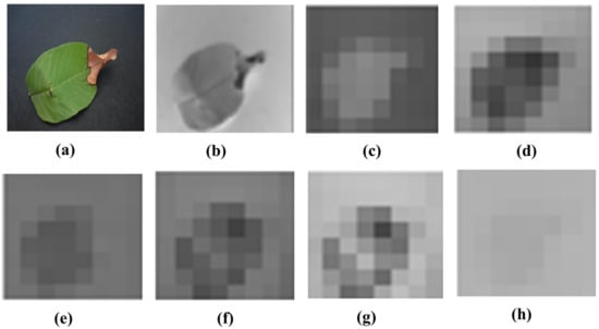
Figure 4. Visualization of the images of strong feature maps of different convolution layers. (a) conv_1 (b) conv_ 2 (c) conv_ 3 (d) conv_4 (e) conv_5 (f) conv_6 (g) conv_7 (h) conv2.

3.5. DarkNet-53

DarkNet-53 acts as the backbone of YoloV3 for object detection. DarkNet comprises 53 layers and consists of multiple convolution layers. A total of 1024 features in DarkNet are extracted with the help of the global average pooling layer. There are 25 layers in Batch normalization. The input size is 256 × 256. According to our mathematical model, the features in DarkNet are presented as:

$$f_{a\times b}=\{ j1\times 1 , j1\times 2 , j1\times 3 ,\dots \dots \dots \dots ..j1\times m \}$$

(8)

where J (_1…m) shows the number of features extracted from DarkNet-53 and a × b is the dimension of the resultant function. Visualization of the strongest feature maps at different convolution layers with the DarkNet-53 architecture is shown in Figure 5

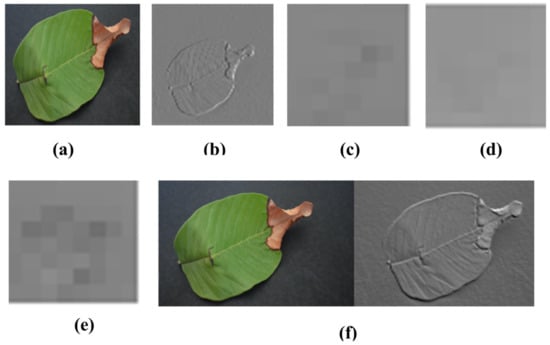
Figure 5. Visualization of the images of strong feature maps of different convolution layers of DarkNet-53. (a) conv3 (b) conv1 (c) conv2 (d) conv4 (e) conv5 (f) conv6.

3.6. AlexNet

AlexNet is the simplest model that comprises 8 layers. There are 5 convolution layers and 3 fully connected layers. Its input size is 227 × 227. The Activation function used in all layers is ReLU, which is applied after every convolution layer and fully connected layer. The Drop layer is applied after the first and second fully connected layer. The Activation function in the output layer is Softmax. The AlexNet contains 4096 features with the help of a convolution layer named a fully connected layer. According to our mathematical model, the features in AlexNet are presented as:

$$f_{c\times d }=\{ k_{1\times 1}, k_{1\times 2}, k1\times 3, \dots \dots .k1\times n\}$$

(9)

where k(1 … n) shows the number of features extracted from AlexNet and c × d shows the dimensions of the resultant function. Visualization of the strongest feature maps at different convolution layers with the AlexNet architecture is shown in Figure 6

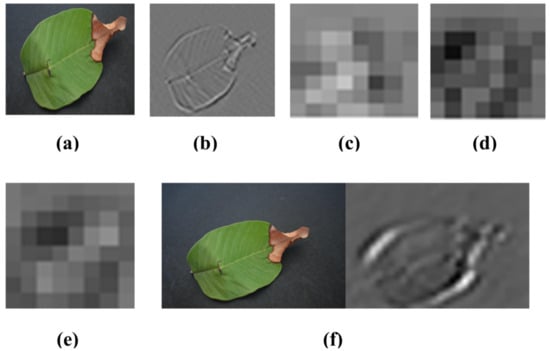
Figure 6. Visualization of the images of strong feature maps of different convolution layers of AlexNet. (a) conv2 (b) conv1 (c) conv3 (d) conv4 (e) conv5 (f) conv6.

3.7. Feature Selection

After extracting features from the proposed model and other pretrained models such as DarkNet-53, AlexNet, and SidNet, the selection of features is done with the help of feature sorting using entropy. The mathematical model for the selection of features using entropy is represented as:

$$E_{a\times b }\left({ᾳ}_1, {ᾳ}_2, {ᾳ}_3, \dots .. {ᾳ}_n\right)=-{\displaystyle \sum } fa\times b \{j1\times 1 , j1\times 2, j1\times 3,\dots .j1\times m\}log(j 1\times 1 , j1\times 2 , j1\times 3,\dots \dots j1\times m)$$

(10)

$$E_{c\times d }({\beta }_1, {\beta }_2, {\beta }_3, \dots .. {\beta }_n-{\displaystyle \sum } f_{c\times d}=\{k_{1\times 1},k_{1\times 2},k_{1\times 3},\dots ..k_{1\times n}\}loglog \left(k_{1\times 1} , k_{1\times 2} , k_{1\times 3}, \dots \dots \dots k_{1\times n}\right)$$

(11)

$$E_{e\times f }({\gamma }_1, {\gamma }_2, {\gamma }_3, \dots \dots {\gamma }_n=-{\displaystyle \sum } f_{e\times f}=\{L_{1\times 1},L_{1\times 2},L_{1\times 3,}\dots \dots L_{1\times p}\}loglog \left(L_{1\times 1} , L_{1\times 2} , L_{1\times 3},\dots \dots ..L_{1\times p}\right)$$

(12)

where a × b, c × d, e × f represents the dimension of features obtained after sorting features. Log(j(1 − n)), Log(k(1 − n)), and Log(L(1 − n)) show the prediction of probability and j(1 − n), k(1 − n) and L(1 − n) show the selected features obtained from the extracted features. $ᾳ$ (1 − n), β(1 − n), $\gamma \left(1-n\right)$ show the features which are sorted.

3.8. Feature Fusion

Feature Fusion is performed to select the most optimal features. According to the mathematical model, the fusion of features is represented as:

$$\in f={{\displaystyle \sum }}_{x=1}^L\left( E_{a\times b}\right){\displaystyle \bigcup } {{\displaystyle \sum }}_{y=1}^m\left(E_{c\times d}\right){\displaystyle \bigcup } {{\displaystyle \sum }}_{z=1}^n\left(E_{e\times f}\right)$$

(13)

After fusing the features using the entropy algorithm, Binary Gray Wolf Optimization is performed to obtain the most optimal results. The mathematical model representing the features selected from Binary Gray Wolf Optimization are as follows:

$${\varnothing }^{\mathrm{d}}=\in 1 if \gamma o<\frac{1}{3} \in 2 if \frac{1}{3}\le \gamma 6<\frac{2}{3} \in 3 if , otherwise$$

(14)

where $\varnothing$^d is the function of BGWO and $\gamma o$ and $\gamma 6$ are the adjusting parameters that are used to set the value of the most optimal features.

3.9. Classification

Different classifiers are available for classification purposes, but SVM and KNN classifiers are chosen. These two classifiers are selected to achieve high accuracy and the most optimal results. In machine learning, features are reduced by carrying out the feature vector dimension. Different classification algorithms are available, such as Minimum Mean Distance (MMD), K means clustering, Decision Trees, Shadow algorithm, and Naïve Bayes. In this work, SVM and KNN are selected to perform the classification on the guava leaf dataset. These classifiers generate better results compared to other classifiers.

4. Results and Discussion

The purpose of this study is to classify the Leaf Blight disease with the best possible results. After the processing of the dataset using YCbCr, the extraction of features is performed using two pretrained models along with one proposed net. The selection of features is performed using BGWO. For classification purposes, SVM and KNN are chosen for the evaluation of execution. This section provides details about experiments that are performed on multiple sets of features and the results are recorded accordingly. These experiments and results are shown in two sets of test cases. Using 5 folds and 10 folds, validation experiments are performed. In comparison with other classifiers, SVM and KNN are selected, as they give the best results. The set of experiments are performed on Windows 10 (64-bit) and a Core (TM) i7-8700 CPU, 3.20 GHz (12 CPUs) 3.2 GHz processor with 16 GB RAM and an LCD and keyboard from HP. Training and testing of the designed network are performed on MATLAB R2020b.

4.1. Dataset

The assembled dataset for the classification of Leaf Blight used in this analysis [61] is small. These experiments are performed on guava leaves. The chosen dataset contains 415 guava leaf images in the original. This dataset contains a small number of images; therefore, they are augmented using horizontal and vertical flipping techniques, which increases the total number of images. The total number of images is 1000 after the augmentation technique. This dataset is publicly available on the Mendeley website. It is a binary class dataset (see Figure 7 for sample images) and many researchers have used it in their studies.

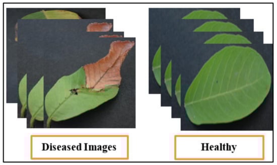
Figure 7. Sample dataset images of guava plant.

4.2. Performance Evaluation Methods

The performance measures can be used to measure and detect the performance of leaf blight disease in plants. The consequences are defined as follows: a True Positive rate as TP, True Negative rate as TN, False Positive rate as FP, and False Negative rate as FN. The Table 2 illustrates the performance measures that are used in this work.

Table 2. Performance evaluation metrics.

Measures	Mathematical Expressions
Accuracy	$\frac{\mathrm{True}\mathrm{Positive}+\mathrm{True}\mathrm{Negative}}{\mathrm{True}\mathrm{Positive}\mathrm{True}\mathrm{Negative}+\mathrm{False}\mathrm{Positive}+\mathrm{False}\mathrm{Negative}}$
Recall	$\frac{\mathrm{True}\mathrm{Positive}}{\mathrm{True}\mathrm{Positive}+\mathrm{False}\mathrm{Positive}}$
PRC/Positive Prediction	$\frac{\mathrm{True}\mathrm{Positive}}{\mathrm{True}\mathrm{Positive}+\mathrm{False}\mathrm{Positive}}$
F1 Score	$\frac{2.\mathrm{Precision}.\mathrm{Recall}}{\mathrm{Precision}+\mathrm{Recall}}$

Table 3 shows a summary of the best-achieved results performed on the guava leaf dataset, which proves that the proposed methodology is efficient and robust. Here, Quadratic SVM achieves the best results, i.e., 98.9% over 5 folds in 9.2 s and 99.2% over 10 folds in 16.2 s, with 3045 features on 5-fold cross validation.

Table 3. Summary of results.

Test Cases	Experiment #	Folds	Features	Classifier	Accuracy %	Training Time (s)
1	1 (a)	5	3045	Quadratic SVM	98.9	9.2
2	2 (a)	5	200	Fine Gaussian SVM	81.1	0.8
3	3 (a)	5	500	Quadratic SVM	84.1	2.2
4	4 (a)	5	750	Cubic SVM	85.6	2.4
5	5 (a)	5	1000	Cubic SVM	87.6	3.2
6	1 (b)	10	3045	Quadratic SVM	99.2	16.2
7	2 (b)	10	200	Fine Gaussian SVM	82.6	1.2
8	3 (b)	10	500	Fine Gaussian SVM	85.2	2.20
9	4 (b)	10	750	Cubic SVM	87.8	4.8
10	5 (b)	10	1000	Cubic SVM	87.5	6.2

The accompanying text contains some discussion on some of the experiments.

• Experiment_1: Using 5-Fold and 10-Fold Validation on 3045 features

This section provides details about two test cases that were performed on 3045 features using both 5 folds and 10 folds. The selected classifiers are variants of SVM and KNN, which were chosen to get robust results. After augmentation, the chosen dataset contained 1002 images. The best results were recorded with measures such as accuracy, precision, recall, F1-score, and training time.

• Experiment_1(a): Using 5 Folds and 3045 Features (1002 × 3045 features)

This test case shows the results of 3045 features upon 1002 images using SVM and KNN classifiers with 5-fold cross validation. Details are shown in Table 4.

Table 4. Experiment_1 using 5 Folds (3045 Feature).

Classifier	Accuracy (%)	Total Cost	Precision Speed (obs/s)	Training Time (s)	Precision	F1-Score	Recall
Quadratic SVM	98.9	12	760	9.21	0.99	0.99	0.99
Linear SVM	98.0	20	780	9.65	0.98	0.98	0.98
Cubic SVM	98.6	14	770	9.43	0.985	0.985	0.99
Fine Gaussian SVM	80.1	199	490	16.3	0.78	0.785	0.86
Medium Gaussian SVM	97.3	27	770	9.76	0.97	0.975	0.97
Coarse Gaussian SVM	92.5	75	740	10.35	0.915	0.925	0.92
Weighted KNN	95.0	50	360	12.89	0.945	0.95	0.95
FINE KNN	93.5	65	360	13.62	0.935	0.935	0.94
Medium KNN	87.8	122	360	12.94	0.865	0.875	0.90
Coarse KNN	81.3	187	360	12.81	0.795	0.795	0.87
Cosine KNN	89.8	101	330	13.52	0.89	0.895	0.91
Cubic KNN	87.5	125	73	58.97	0.865	0.87	0.90

The best results are achieved by the Quadratic SVM classifier in comparison with all KNN classifiers, which is 98.9% in 9.2 s. Here, the confusion matrix in Figure 8 and the ROC curve in Figure 9 are shown for the best results with the Quadratic SVM classifier. In the confusion matrix, A represents the diseased class, While B depicts healthy class

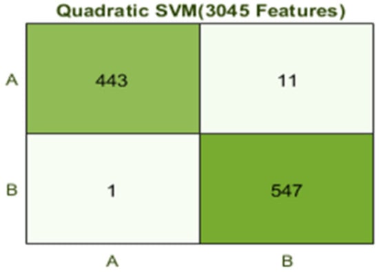
Figure 8. Confusion matrix for Q(SVM) with 3045 features and using 5-fold results.

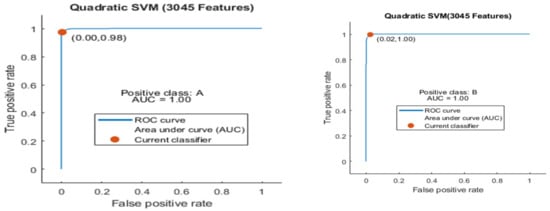
Figure 9. ROC curve for two classes A and B with 3045 features and using 5-fold results.

Here the ROC curve is shown in Figure 9 for both classes A and B, which are presented as ROC A and ROC B.

• Experiment_1(b): Using 10 Folds and 3045 Features (1002 × 3045 features)

This test case shows the results of 3045 features upon 1002 images using SVM and KNN classifiers with 10 folds. Details are shown in Table 5.

Table 5. Experiment_1 using 10 Folds (3045 Feature).

Classifier	Accuracy (%)	Total Cost	Precision Speed (obs/s)	Training Time (s)	Precision	Recall	F1-Score
Quadratic SVM	99.2	8	460	16.221	0.995	0.99	0.99
Linear SVM	98.3	17	440	18.23	0.98	0.98	0.98
Cubic SVM	99.1	9	450	16.7	0.99	0.99	0.99
Fine Gaussian SVM	85.4	146	310	29.265	0.84	0.89	0.84
Medium Gaussian SVM	98.3	17	450	17.676	0.98	0.98	0.98
Coarse Gaussian SVM	93.6	64	450	18.689	0.93	0.94	0.93
Weighted KNN	94.3	57	190	23.037	0.935	0.95	0.94
FINE KNN	94.2	58	190	24.374	0.935	0.95	0.94
Medium KNN	88.2	118	190	23.12	0.87	0.91	0.87
Coarse KNN	82.7	173	190	23.278	0.81	0.88	0.81
Cosine KNN	91.0	90	180	24.438	0.9	0.92	0.90
Cubic KNN	88.3	117	57	73.713	0.87	0.91	0.87

The Quadratic SVM classifier achieved the best result in comparison with all KNN classifiers, which is 99.2%. Here, the confusion matrix as presented in Figure 10 and the ROC curve are shown for the best results against the Quadratic SVM classifier.

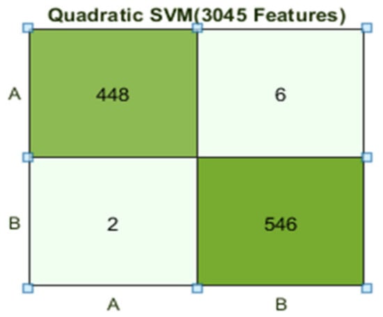
Figure 10. Confusion matrix for Q(SVM) with 3045 features and using 10-fold results.

Here, the ROC curve is shown in Figure 11 for both classes A and B, which are presented as ROC A and ROC B.

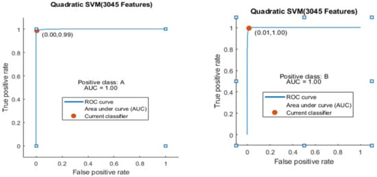
Figure 11. ROC curve for two classes A and B with 3045 features and using 10-fold results.

• Experiment_2: Using 5-Fold and 10-Fold Validation on 200 features

This section provides details about two test cases that were performed on 200 features using both 5 folds and 10 folds. The efficiently selected classifiers are SVM and KNN, which were chosen to get robust results. The chosen dataset contains 1002 images. The best results are recorded with other measures, such as accuracy, precision, recall, F1-score, training time, etc. Results are shown in the Table 6 in detail.

Table 6. Experiment_2 using 5 Folds (200 Feature).

Classifier	Accuracy (%)	Total Cost	Precision Speed (obs/s)	Training Time (s)	Precision	Recall	F1-Score
Fine Gaussian SVM	81.1	189	14,000	0.81571	0.8	0.82	0.805
Linear SVM	73.7	264	16,000	1.3486	0.735	0.735	0.73
Cubic SVM	80.4	210	15,000	1.8572	0.805	0.805	0.8
Quadratic SVM	78.4	216	15,000	1.7431	0.785	0.78	0.785
Medium Gaussian SVM	72.8	273	15,000	0.7667	0.71	0.74	0.715
Coarse Gaussian SVM	60.5	396	14,000	0.671	0.565	0.71	0.5
Weighted KNN	78.2	218	7700	0.76741	0.785	0.785	0.78
FINE KNN	74.8	253	7600	1.1917	0.75	0.75	0.75
Medium KNN	66.8	333	7800	0.8367	0.66	0.665	0.66
Coarse KNN	62.4	377	7200	0.79092	0.59	0.675	0.555
Cosine KNN	67.2	329	7500	0.766606	0.67	0.665	0.67
Cubic KNN	69.0	311	1200	3.8096	0.68	0.685	0.68

• Experiment_2(a): Using 5 Folds and 200 Features (1002 × 200 features)

This test case shows the results of 200 features upon 1002 images using SVM and KNN classifiers with 5 folds. Details are shown in Table 6.

The Fine Gaussian SVM classifier achieved the best result in comparison with all KNN classifiers, which is 81.1% in 0.8 s. Here, the confusion matrix in Figure 12 and the ROC in Figure 13 curve are shown for the best results with the Fine Gaussian SVM classifier.

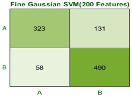
Figure 12. Confusion matrix for FG(SVM) with 200 features and using 5-fold results.

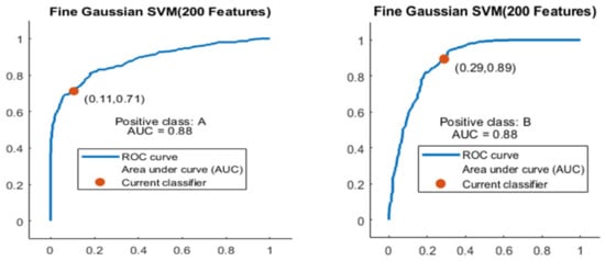
Figure 13. ROC curves for two classes A and B with 200 features and using 5-fold results.

The ROC curve is shown in Figure 13 for both classes A and B which are presented as ROC A and ROC B.

• Experiment_2(b): Using 10 Folds and 200 Features (1002 × 200 features)

This test case shows the results of 200 features upon 1002 images using SVM and KNN classifiers with 10 folds. Details are shown in Table 7.

Table 7. Experiment_2 using 10 Folds (200 Feature).

Classifier	Accuracy (%)	Total Cost	Precision Speed (obs/s)	Training Time (s)	Precision	Recall	F1-Score
Fine Gaussian SVM	82.6	174	8300	1.2664	0.815	0.83	0.825
Linear SVM	73.2	269	8000	1.8576	0.725	0.73	0.73
Cubic SVM	80.8	192	8400	5.6548	0.815	0.81	0.81
Quadratic SVM	78.2	218	7800	3.4237	0.78	0.78	0.78
Medium Gaussian SVM	73.9	262	8100	1.15	0.725	0.75	0.725
Coarse Gaussian SVM	60.2	399	8100	1.1668	0.565	0.715	0.49
Weighted KNN	78.6	214	4100	1.2662	0.79	0.785	0.78
FINE KNN	75.0	250	4200	1.8358	0.755	0.75	0.75
Medium KNN	65.9	342	4000	1.8129	0.655	0.655	0.65
Coarse KNN	62.0	381	4000	1.2544	0.59	0.67	0.55
Cosine KNN	65.9	342	3900	1.274	0.665	0.665	0.655
Cubic KNN	68.5	316	960	4.57	0.675	0.68	0.68

Here, the Fine Gaussian SVM classifier achieved the best result in comparison with all KNN classifiers, which is 82.6% in 1.2 s. Here, the confusion matrix also shown in Figure 14 and the ROC curve are shown for the best results against the Fine Gaussian SVM classifier.

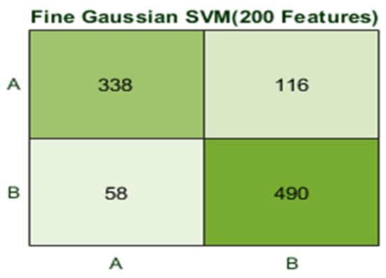
Figure 14. Confusion matrix for FG(SVM) with 200 features and using 10-fold results.

The ROC curve is shown in Figure 15 for both classes A and B, which are presented as ROC A and ROC B.

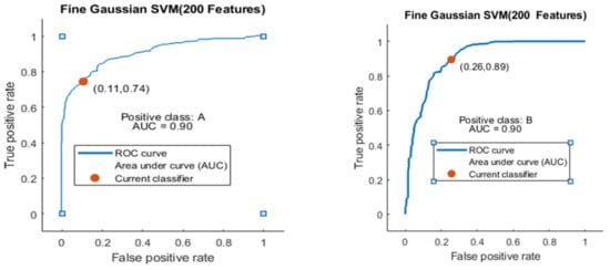
Figure 15. ROC curve for two classes A and B with 200 features and using 10-fold results.

• Experiment_3: Using 5-Fold and 10-Fold Validation on 500 features.

This section provides details about two test cases that are performed on 500 features using both 5 folds and 10 folds. The efficiently selected classifiers are SVM and KNN, which were chosen to get robust results. The chosen dataset contains 1002 images. The best results are recorded with some other measures like Accuracy, precision, recall, F1-score, training time, and others. Results are shown in the Table 8 in detail.

Table 8. Experiment_3 using 5 Folds (500 Feature).

Classifier	Accuracy (%)	Total Cost	Precision Speed (obs/s)	Training Time (s)	Precision	Recall	F1-Score
Quadratic SVM	84.1	159	7000	2.2045	0.84	0.84	0.84
Linear SVM	79.0	210	6900	1.7001	0.785	0.79	0.79
Cubic SVM	82.4	176	7300	2.2117	1.64	1.65	1.65
Fine Gaussian SVM	83.6	164	6900	1.2768	1.66	1.68	1.67
Medium Gaussian SVM	75.8	242	6900	1.1461	0.745	0.765	0.75
Coarse Gaussian SVM	67.0	331	6800	1.1891	0.65	0.68	0.65
Weighted KNN	80.4	196	3100	1.5885	0.805	0.805	0.805
FINE KNN	77.6	224	3200	1.9972	0.78	0.775	0.775
Medium KNN	69.4	307	3200	1.6358	0.685	0.69	0.685
Coarse KNN	67.4	331	3100	1.584	0.65	0.695	0.64
Cosine KNN	68.5	316	3000	1.6165	0.685	0.685	0.685
Cubic KNN	73.3	268	470	9.3325	0.72	0.73	0.73

• Experiment_3(a): Using 5 Folds and 500 Features (1002 × 500 features)

This test case shows the results of 500 features upon 1002 images using SVM and KNN classifiers with 5 folds. Details are shown in Table 8.

Here, the classifier Quadratic SVM achieved the best result in comparison with all KNN classifiers, which is 84.1% in 1.2 s. The confusion matrix in Figure 16 and the ROC curve in Figure 17 are shown for the best results against the Quadratic SVM classifier.

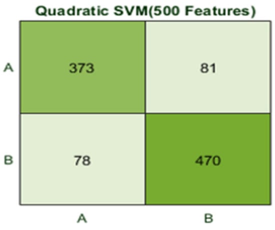
Figure 16. Confusion matrix for Q(SVM) with 500 features and using 500 fatures with 5-fold results.

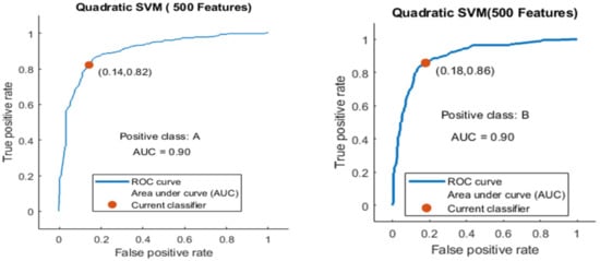
Figure 17. ROC curve for two classes A and B with 500 features and using 5-fold results.

The ROC curve is shown for both classes A and B, which are presented as ROC A and ROC B in Figure 17.

• Experiment_3(b): Using 10 Folds and 500 Features (1002 × 500 features)

This test case shows the results of 500 features upon 1002 images using SVM and KNN classifiers with 10 folds. Details are shown in Table 9.

Table 9. Experiment_3 using 10 Folds (500 Feature).

Classifier	Accuracy (%)	Total Cost	Precision Speed (obs/sec)	Training Time (s)	Precision	Recall	F1-Score
Fine Gaussian SVM	85.2	148	3800	2.2088	0.845	0.86	0.85
Linear SVM	79.8	202	3600	4.5137	0.79	0.8	0.79
Cubic SVM	84.2	158	4100	4.4002	0.845	0.84	0.84
Quadratic SVM	84.7	153	4000	4.1644	0.845	0.845	0.845
Medium Gaussian SVM	75.9	241	4000	2.1057	0.75	0.765	0.755
Coarse Gaussian SVM	67.7	324	3900	2.0635	0.66	0.69	0.655
Weighted KNN	82.5	175	1800	2.6916	0.83	0.825	0.825
FINE KNN	79.4	206	1700	3.7172	0.795	0.795	0.79
Medium KNN	71.5	286	1800	2.7012	0.71	0.71	0.71
Coarse KNN	66.4	337	1800	2.667	0.645	0.685	0.63
Cosine KNN	67.9	322	1600	2.786	0.685	0.68	0.68
Cubic KNN	75.4	246	380	11.154	0.75	0.75	0.75

Here, the classifier Fine Gaussian SVM achieved the best result in comparison with all KNN classifiers, which is 85.2% in 2.2 s. Here, the confusion matrix and the ROC curve are shown for the best results against the Fine Gaussian SVM classifier. The confusion matrix for FG (SVM) is shown in Figure 18.

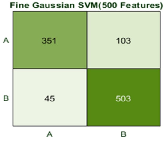
Figure 18. Confusion matrix for FG(SVM) with 500 features and using 10-fold results.

Here, the ROC curve is presented (in Figure 19) for both classes A and B, which are presented as ROC A and ROC B.

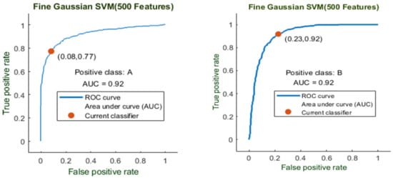
Figure 19. ROC curve for two classes A and B with 500 features and using 10-fold results.

Figure 20 shows the 5-fold best achievable results between training time and features. It shows the consumed time for training that is required for a particular set of features.

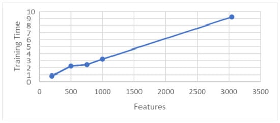
Figure 20. Graph showing training time and features on 5-fold.

Here, features are presented on the x-axis and the training time is shown on the y-axis. These results are taken on 5-folds for the best achievable results.

Similarly, the graph in Figure 21 shows the relation between accuracy and features at 5-fold results. It shows that the features are presented along the x-axis and the accuracy is presented along the y-axis, and the line presents the best achievable results.

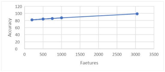
Figure 21. Graph showing accuracy and features on 5-fold.

The graph in Figure 22 shows the relation between training time and features upon results taken on 10 folds. This graph shows that features are shown along the x-axis and the training time is shown along the y-axis, and the time consumed by a particular set of features for training is illustrated.

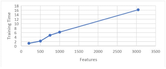
Figure 22. Graph showing features and training time.

The graph in Figure 23 shows the relation between training time and accuracy upon results taken on 10 folds. This graph shows that features are shown along the x-axis and the accuracy is shown along the y-axis, and the time consumed by a particular set of features for training is illustrated.

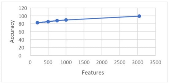
Figure 23. Graph showing features and accuracy on 10 folds.

5. Conclusions

Agriculture is the key to the development and rise of emergent nations. Diseases in plants cause crop damage. Detection of leaf blight is enormously important as it affects the annual production of guava fruit. Finally, the development of an automated system becomes indispensable. In this paper, leaf blight can be detected, analyzed, and classified through the proposed methodology. In this proposed methodology, our own deep CNN is designed, containing thirty-three layers. In the first phase of image processing, preprocessing is done by using color spacing YCbCr. The Guava dataset is chosen for the identification and analysis of leaf blight. Because the dataset is small, data augmentation is performed. Horizontal and vertical flipping were performed on images of guava leaves. After preprocessing, feature extraction was performed using Darknet-53 and AlexNet, as well as the proposed SidNet. For the selection of the best features, optimization algorithms such as Entropy and Binary Gray Wolf are used. Finally, classification is performed on guava leaf images and the best results with higher accuracy and less computational cost are achieved. Multiple experiments are performed while using the set of selected features (200, 500, 750, 1000 features using 5- and 10-fold validation). Based on the selected features, 98.9% of the results are achieved using an SVM classifier, as it proves that this proposed methodology is robust and efficient.

In the future, this work can be explored with quantum deep learning for improved performance. Quantum computing-based machine learning and deep convolutional neural networks can detect and classify leaf blight at its initial stage more precisely and meticulously, which will help save crops and fruits, save plants from destruction, and increase the production of guava fruit.

References

- Rehman, A.; Jingdong, L.; Shahzad, B.; Chandio, A.A.; Hussain, I.; Nabi, G.; Iqbal, M.S. Economic perspectives of major field crops of Pakistan: An empirical study. Pac. Sci. Rev. B Humanit. Soc. Sci. 2015, 1, 145–158. [Google Scholar] [CrossRef]
- Rai, M.K.; Asthana, P.; Jaiswal, V.; Jaiswal, U. Biotechnological advances in guava (Psidium guajava L.): Recent developments and prospects for further research. Trees 2010, 24, 1–12. [Google Scholar] [CrossRef]
- Mitra, S.; Thingreingam Irenaeus, K. Guava cultivars of the world. In International Symposia on Tropical and Temperate Horticulture—ISTTH2016; CIRAD Publications: Cairns, Queensland, Australia, 2016; pp. 905–910. [Google Scholar]
- Almadhor, A.; Rauf, H.T.; Lali, M.I.U.; Damaševičius, R.; Alouffi, B.; Alharbi, A. AI-Driven Framework for Recognition of Guava Plant Diseases through Machine Learning from DSLR Camera Sensor Based High Resolution Imagery. Sensors 2021, 21, 3830. [Google Scholar] [CrossRef] [PubMed]
- Misra, A. Guava diseases—Their symptoms, causes and management. In Diseases of Fruits and Vegetables; Springer: Berlin/Heidelberg, Germany, 2004; Volume II, pp. 81–119. [Google Scholar]
- Dhiman, B.; Kumar, Y.; Hu, Y.-C. A general purpose multi-fruit system for assessing the quality of fruits with the application of recurrent neural network. Soft Comput. 2021, 25, 9255–9272. [Google Scholar] [CrossRef]
- Ashraf, R.; Habib, M.A.; Akram, M.; Latif, M.A.; Malik, M.S.A.; Awais, M.; Dar, S.H.; Mahmood, T.; Yasir, M.; Abbas, Z. Deep convolution neural network for big data medical image classification. IEEE Access 2020, 8, 105659–105670. [Google Scholar] [CrossRef]
- Naranjo-Torres, J.; Mora, M.; Hernández-García, R.; Barrientos, R.J.; Fredes, C.; Valenzuela, A. A review of convolutional neural network applied to fruit image processing. Appl. Sci. 2020, 10, 3443. [Google Scholar] [CrossRef]
- Lloret, E.; Plaza, L.; Aker, A. The challenging task of summary evaluation: An overview. Lang. Resour. Eval. 2018, 52, 101–148. [Google Scholar] [CrossRef]
- Bojer, C.S.; Meldgaard, J.P. Kaggle forecasting competitions: An overlooked learning opportunity. Int. J. Forecast. 2021, 37, 587–603. [Google Scholar] [CrossRef]
- Fu, X.; Cao, X. Underwater image enhancement with global–local networks and compressed-histogram equalization. Signal Process. Image Commun. 2020, 86, 115892. [Google Scholar] [CrossRef]
- Tang, Z.; Gao, Y.; Karlinsky, L.; Sattigeri, P.; Feris, R.; Metaxas, D. OnlineAugment: Online Data Augmentation with Less Domain Knowledge; Springer: Berlin/Heidelberg, Germany, 2020; pp. 313–329. [Google Scholar]
- Liu, Z.; Lai, Z.; Ou, W.; Zhang, K.; Zheng, R. Structured optimal graph based sparse feature extraction for semi-supervised learning. Signal Process. 2020, 170, 107456. [Google Scholar] [CrossRef]
- Ghojogh, B.; Samad, M.N.; Mashhadi, S.A.; Kapoor, T.; Ali, W.; Karray, F.; Crowley, M. ‘Feature selection and feature extraction in pattern analysis: A literature review. arXiv 2019, arXiv:1905.02845. [Google Scholar]
- Zhang, J.; Liu, B. A review on the recent developments of sequence-based protein feature extraction methods. Curr. Bioinform. 2019, 14, 190–199. [Google Scholar] [CrossRef]
- Latif, A.; Rasheed, A.; Sajid, U.; Ahmed, J.; Ali, N.; Ratyal, N.I.; Zafar, B.; Dar, S.H.; Sajid, M.; Khalil, T. Content-based image retrieval and feature extraction: A comprehensive review. Math. Probl. Eng. 2019, 2019, 9658350. [Google Scholar] [CrossRef]
- Raj, R.J.S.; Shobana, S.J.; Pustokhina, I.V.; Pustokhin, D.A.; Gupta, D.; Shankar, K. Optimal feature selection-based medical image classification using deep learning model in internet of medical things. IEEE Access 2020, 8, 58006–58017. [Google Scholar] [CrossRef]
- Ali, L.; Wajahat, I.; Golilarz, N.A.; Keshtkar, F.; Bukhari, S.A.C. ‘LDA–GA–SVM: Improved hepatocellular carcinoma prediction through dimensionality reduction and genetically optimized support vector machine. Neural Comput. Appl. 2021, 33, 2783–2792. [Google Scholar] [CrossRef]
- Ozyurt, B.; Akcayol, M.A. A new topic modeling based approach for aspect extraction in aspect based sentiment analysis: SS-LDA. Expert Syst. Appl. 2021, 168, 114231. [Google Scholar] [CrossRef]
- Zhao, J.; Liang, J.-M.; Dong, Z.-N.; Tang, D.-Y.; Liu, Z. Accelerating information entropy-based feature selection using rough set theory with classified nested equivalence classes. Pattern Recognit. 2020, 107, 107517. [Google Scholar] [CrossRef]
- Maleki, N.; Zeinali, Y.; Niaki, S.T.A. A k-NN method for lung cancer prognosis with the use of a genetic algorithm for feature selection. Expert Syst. Appl. 2021, 164, 113981. [Google Scholar] [CrossRef]
- Hu, P.; Pan, J.-S.; Chu, S.-C. Improved binary grey wolf optimizer and its application for feature selection. Knowl. Based Syst. 2020, 195, 105746. [Google Scholar] [CrossRef]
- Tubishat, M.; Idris, N.; Shuib, L.; Abushariah, M.A.; Mirjalili, S. Improved Salp Swarm Algorithm based on opposition based learning and novel local search algorithm for feature selection. Expert Syst. Appl. 2020, 145, 113122. [Google Scholar] [CrossRef]
- Too, J.; Rahim Abdullah, A. Binary atom search optimisation approaches for feature selection. Connect. Sci. 2020, 32, 406–430. [Google Scholar] [CrossRef]
- Özyurt, F. A fused CNN model for WBC detection with MRMR feature selection and extreme learning machine. Soft Comput. 2020, 24, 8163–8172. [Google Scholar] [CrossRef]
- De Silva, K.; Jönsson, D.; Demmer, R.T. A combined strategy of feature selection and machine learning to identify predictors of prediabetes. J. Am. Med. Inform. Assoc. 2020, 27, 396–406. [Google Scholar] [CrossRef] [PubMed]
- Germain, P.-L.; Sonrel, A.; Robinson, M.D. pipeComp, a general framework for the evaluation of computational pipelines, reveals performant single cell RNA-seq preprocessing tools. Genome Biol. 2020, 21, 1–28. [Google Scholar] [CrossRef]
- Kaur, P.; Singh, A.; Chana, I. Computational techniques and tools for omics data analysis: State-of-the-art, challenges, and future directions. Arch. Comput. Methods Eng. 2021, 28, 4595–4631. [Google Scholar] [CrossRef]
- Ghosh, P.; Azam, S.; Jonkman, M.; Karim, A.; Shamrat, F.J.M.; Ignatious, E.; Shultana, S.; Beeravolu, A.R.; De Boer, F. Efficient Prediction of Cardiovascular Disease Using Machine Learning Algorithms With Relief and LASSO Feature Selection Techniques. IEEE Access 2021, 9, 19304–19326. [Google Scholar] [CrossRef]
- Deepa, N.; Prabadevi, B.; Maddikunta, P.K.; Gadekallu, T.R.; Baker, T.; Khan, M.A.; Tariq, U. An AI-based intelligent system for healthcare analysis using Ridge-Adaline Stochastic Gradient Descent Classifier. J. Supercomput. 2021, 77, 1998–2017. [Google Scholar] [CrossRef]
- Amini, F.; Hu, G. A two-layer feature selection method using genetic algorithm and elastic net. Expert Syst. Appl. 2021, 166, 114072. [Google Scholar] [CrossRef]
- Zhang, H.; Xu, H.; Xiao, Y.; Guo, X.; Ma, J. Rethinking the Image Fusion: A Fast Unified Image Fusion Network Based on Proportional Maintenance of Gradient and Intensity. Proc. AAAI Conf. Artif. Intell. 2020, 34, 12797–12804. [Google Scholar] [CrossRef]
- Jung, H.; Kim, Y.; Jang, H.; Ha, N.; Sohn, K. Unsupervised deep image fusion with structure tensor representations. IEEE Trans. Image Process. 2020, 29, 3845–3858. [Google Scholar] [CrossRef]
- Shakya, S. Analysis of artificial intelligence based image classification techniques. J. Innov. Image Process. (JIIP) 2020, 2, 44–54. [Google Scholar] [CrossRef]
- Hong, D.; Wu, X.; Ghamisi, P.; Chanussot, J.; Yokoya, N.; Zhu, X.X. Invariant attribute profiles: A spatial-frequency joint feature extractor for hyperspectral image classification. IEEE Trans. Geosci. Remote Sens. 2020, 58, 3791–3808. [Google Scholar] [CrossRef]
- Ke, Z.; Qiu, D.; Li, K.; Yan, Q.; Lau, R.W. Guided Collaborative Training for Pixel-Wise Semi-Supervised Learning; Springer: Berlin/Heidelberg, Germany, 2020; pp. 429–445. [Google Scholar]
- Wang, F.; Liu, H.; Guo, D.; Sun, F. Unsupervised Representation Learning by InvariancePropagation. arXiv 2020, preprint. arXiv:2010.11694. [Google Scholar]
- Karantanellis, E.; Marinos, V.; Vassilakis, E.; Christaras, B. Object-based analysis using unmanned aerial vehicles (UAVs) for site-specific landslide assessment. Remote Sens. 2020, 12, 1711. [Google Scholar] [CrossRef]
- Durmuş, H.; Güneş, E.O.; Kırcı, M. Disease Detection on the Leaves of the Tomato Plants by Using Deep Learning; IEEE: Piscataway, NJ, USA, 2017; pp. 1–5. [Google Scholar]
- Atila, Ü.; Uçar, M.; Akyol, K.; Uçar, E. Plant leaf disease classification using EfficientNet deep learning model. Ecol. Inform. 2021, 61, 101182. [Google Scholar] [CrossRef]
- Ferentinos, K.P. Deep learning models for plant disease detection and diagnosis. Comput. Electron. Agric. 2018, 145, 311–318. [Google Scholar] [CrossRef]
- Azarmdel, H.; Jahanbakhshi, A.; Mohtasebi, S.S.; Muñoz, A.R. Evaluation of image processing technique as an expert system in mulberry fruit grading based on ripeness level using artificial neural networks (ANNs) and support vector machine (SVM). Postharvest Biol. Technol. 2020, 166, 111201. [Google Scholar] [CrossRef]
- Kasinathan, T.; Singaraju, D.; Uyyala, S.R. Insect classification and detection in field crops using modern machine learning techniques. Inf. Process. Agric. 2021, 8, 446–457. [Google Scholar] [CrossRef]
- Yao, J.; Ye, Y. The effect of image recognition traffic prediction method under deep learning and naive Bayes algorithm on freeway traffic safety. Image Vis. Comput. 2020, 103, 103971. [Google Scholar] [CrossRef]
- Atouf, I.; Al Okaishi, W.Y.; Zaaran, A.; Slimani, I.; Benrabh, M. A real-time system for vehicle detection with shadow removal and vehicle classification based on vehicle features at urban roads. Int. J. Power Electron. Drive Syst. 2020, 11, 2091. [Google Scholar] [CrossRef]
- Khan, M.A.; Khan, M.A.; Ahmed, F.; Mittal, M.; Goyal, L.M.; Hemanth, D.J.; Satapathy, S.C. Gastrointestinal diseases segmentation and classification based on duo-deep architectures. Pattern Recognit. Lett. 2020, 131, 193–204. [Google Scholar] [CrossRef]
- Chen, J.; Lian, Y.; Li, Y. ‘Real-time grain impurity sensing for rice combine harvesters using image processing and decision-tree algorithm. Comput. Electron. Agric. 2020, 175, 105591. [Google Scholar] [CrossRef]
- Moubayed, A.; Injadat, M.; Shami, A.; Lutfiyya, H. Student engagement level in an e-learning environment: Clustering using k-means. Am. J. Distance Educ. 2020, 34, 137–156. [Google Scholar] [CrossRef]
- Nanglia, P.; Kumar, S.; Mahajan, A.N.; Singh, P.; Rathee, D. A hybrid algorithm for lung cancer classification using SVM and Neural Networks. ICT Express 2021, 7, 335–341. [Google Scholar] [CrossRef]
- Wu, W.; Li, D.; Du, J.; Gao, X.; Gu, W.; Zhao, F.; Feng, X.; Yan, H. An intelligent diagnosis method of brain MRI tumor segmentation using deep convolutional neural network and SVM algorithm. Comput. Math. Methods Med. 2020, 2020, 6789306. [Google Scholar] [CrossRef]
- Basha, C.Z.; Rohini, G.; Jayasri, A.V.; Anuradha, S. Enhanced and Effective Computerized Classification of X-Ray Images; IEEE: Piscataway, NJ, USA, 2020; pp. 86–91. [Google Scholar]
- Islam, N.; Rashid, M.M.; Wibowo, S.; Xu, C.-Y.; Morshed, A.; Wasimi, S.A.; Moore, S.; Rahman, S.M. Early Weed Detection Using Image Processing and Machine Learning Techniques in an Australian Chilli Farm. Agriculture 2021, 11, 387. [Google Scholar] [CrossRef]
- Sasankar, P.; Kosarkar, U. A Study for Face Recognition Using Techniques PCA and KNN. EasyChair Print. 2021. Available online: https://wwww.easychair.org/publications/preprint_download/gS7Q (accessed on 30 January 2023).
- Bharate, A.A.; Shirdhonkar, M. Classification of Grape Leaves Using KNN and SVM Classifiers; IEEE: Piscataway, NJ, USA, 2020; pp. 745–749. [Google Scholar]
- Goncharov, P.; Ososkov, G.; Nechaevskiy, A.; Uzhinskiy, A.; Nestsiarenia, I. Disease Detection on the Plant Leaves by Deep Learning; Springer: Berlin/Heidelberg, Germany, 2018; pp. 151–159. [Google Scholar]
- De Luna, R.G.; Dadios, E.P.; Bandala, A.A. Automated Image Capturing System for Deep Learning-Based Tomato Plant Leaf Disease Detection and Recognition; IEEE: Piscataway, NJ, USA, 2018; pp. 1414–1419. [Google Scholar]
- Sharma, P.; Berwal, Y.P.S.; Ghai, W. Performance analysis of deep learning CNN models for disease detection in plants using image segmentation. Inf. Process. Agric. 2020, 7, 566–574. [Google Scholar] [CrossRef]
- Oppenheim, D.; Shani, G.; Erlich, O.; Tsror, L. Using deep learning for image-based potato tuber disease detection. Phytopathology 2019, 109, 1083–1087. [Google Scholar] [CrossRef]
- Chowdhury, M.E.; Rahman, T.; Khandakar, A.; Ayari, M.A.; Khan, A.U.; Khan, M.S.; Al-Emadi, N.; Reaz, M.B.I.; Islam, M.T.; Ali, S.H.M. Automatic and Reliable Leaf Disease Detection Using Deep Learning Techniques. AgriEngineering 2021, 3, 294–312. [Google Scholar] [CrossRef]
- Krizhevsky, A.; Hinton, G. Learning Multiple Layers of Features from Tiny Images. 2009. Available online: http://www.cs.utoronto.ca/~kriz/learning-features-2009-TR.pdf (accessed on 30 January 2023).
- Rauf, H.T.; Lali, M.I.U. A Guava Fruits and Leaves Dataset for Detection and Classification of Guava Diseases through Machine Learning. Mendeley Data 2021, 1. (Dataset). [Google Scholar]
Disclaimer/Publisher’s Note: The statements, opinions and data contained in all publications are solely those of the individual author(s) and contributor(s) and not of MDPI and/or the editor(s). MDPI and/or the editor(s) disclaim responsibility for any injury to people or property resulting from any ideas, methods, instructions or products referred to in the content. |
© 2023 by the authors. Licensee MDPI, Basel, Switzerland. This article is an open access article distributed under the terms and conditions of the Creative Commons Attribution (CC BY) license (https://creativecommons.org/licenses/by/4.0/).