Article

Leveraging Important Covariate Groups for Corn Yield Prediction

1
Department of Plants, Soils and Climate and Ecology Center, Utah State University, 4820 Old Main Hill, Logan, UT 84322-4820, USA
2
Department of Environmental Sciences, Emory University, 400 Dowman Drive, Atlanta, GA 30322, USA
3
Department of Mathematics and Statistics, Utah State University, 3900 Old Main Hill, Logan, UT 84322-3900, USA
4
Agroclimate Extension Specialist, Department of Plants, Soils and Climate, Utah State University, 4820 Old Main Hill, Logan, UT 84322-4820, USA
*
Author to whom correspondence should be addressed.
Agriculture 2023, 13(3), 618; https://doi.org/10.3390/agriculture13030618
Submission received: 23 January 2023 / Revised: 26 February 2023 / Accepted: 2 March 2023 / Published: 3 March 2023

Abstract

:
Accurate yield information empowers farmers to adapt, their governments to adopt timely agricultural and food policy interventions, and the markets they supply to prepare for production shifts. Unfortunately, the most representative yield data in the US, provided by the US Department of Agriculture, National Agricultural Statistics Service (USDA-NASS) Surveys, are spatiotemporally patchy and inconsistent. This paper builds a more complete data product by examining the spatiotemporal efficacy of random forests (RF) in predicting county-level yields of corn—the most widely cultivated crop in the US. To meet our objective, we compare RF cross-validated prediction accuracy using several combinations of explanatory variables. We also utilize variable importance measures and partial dependence plots to compare and contextualize how key variables interact with corn yield. Results suggest that RF predicts US corn yields well using a relatively small subset of climate variables along with year and geographical location (RMSE = 17.1 bushels/acre (1.2 tons/hectare)). Of note is the insensitivity of RF prediction accuracy when removing variables traditionally thought to be predictive of yield or variables flagged as important by RF variable importance measures. Understanding what variables are needed to accurately predict corn yields provides a template for applying machine learning approaches to estimate county-level yields for other US crops.

1. Introduction

In the coterminous US, 55 percent of the land is dedicated to food production, with two-thirds of all cropland cultivated with one of three major crops: corn, wheat, or soybean [1]. Over the last century, corn yields have increased fivefold. These yield gains have been driven by technological innovations in agriculture and political–economic incentivization. Despite continuing advances in agricultural technologies and policies built to protect farmers, research suggests that climate change and variability is already impacting agricultural yields [2,3] and that future climate changes are sure to exacerbate challenges to agricultural production. For instance, increased exposure to stressful temperatures is projected to significantly decrease corn yields in many regions of the US [4,5,6]; by one estimation, a 5 °C increase in temperature could cause catastrophic corn yield declines between 30 and 50% [7].
Crop yield variability and change and its determinants are of major concern to farmers, their governments, and the markets they supply [8]. Without accurate yield information, it is nearly impossible for markets to prepare for production shifts, for farmers to adapt to future cropscapes, or for governments to make timely policy interventions; and without knowledge of crop yield determinants across space-time, it is difficult to target future scientific research efforts or inform farmers of broad patterns in yield response to manageable on-farm variables. Unfortunately, the most accurate and spatiotemporally available yield data in the US, provided by the US Department of Agriculture, National Agricultural Statistics Service (USDA-NASS) Surveys, are incomplete, missing key data, and are not attached to features important to agricultural yield. These spatiotemporal data limitations arise due to different sampling protocols used for data collection (i.e., states do not always sample respondents in the same way), question-level non-responses (i.e., farmer’s inability and/or unwillingness to answer questions despite their applicability to all respondents), disclosure requirements, and a seemingly limitless body of covariates known to influence yield at varying scales.
In a comprehensive sweep of USDA-NASS Survey yield data for corn between 2008 and 2018, 25.4% of US county-year data is missing in the coterminous US in counties reporting at least one year of corn yields during that period (n = 2076; Figure S1). Across all 3108 counties, including those that reported no corn yields, 50.2% of yield data is missing. These counties may be “missing” because they produced no corn, or, more likely, because there were not enough reporting growers to meet NASS statistical disclosure requirements. These disclosure requirements ensure that grower confidentiality is maintained, and we commend NASS for upholding them. At the same time, we recognize the expansion of statistical possibilities that come with more complete yield data, especially when that data is made freely accessible for the common good.
This paper offers a framework for building an open-source and more complete yield dataset without threatening confidential grower information. In these counties where data is missing, or where corn is not currently grown, we utilize blended data from big (i.e., remotely sensed) and traditional (i.e., censuses and surveys) sources, in concert with statistical models, to build an infilled yield dataset. The data we have access to limits what we can know about US agriculture [9]. Thus, by producing this infilled dataset, which we can think of as mapping “anticipated production”, we can increase our understanding of US agriculture and help farmers better consider expanding or contracting their cultivated acreage in response to changing cropscapes and geographies. Counties in which corn production was not previously viable (biophysically or economically) may become viable as the climate changes; and those areas that are currently highly productive (e.g., the US Corn Belt), may collapse entirely [10]. We must prepare farmers for these changes; and monitoring how crop yield and crop yield predictions change through time and across space in relation to features of interest is one way to do so.
In recent decades, crop yield studies have moved in the direction of empirical modeling, utilizing statistical modeling techniques to estimate the relationship between crop yield and important determinants of yield (e.g., precipitation, temperature). These empirical models do not consider the underlying physiological processes that govern below or above-ground plant growth as process-based, mechanistic, biophysical models do (see [11] for a review), yet still provide quite reasonable estimations of crop yield [12]. In fact, when predicting at large spatial scales, statistical models generally outperform mechanistic models [11,12,13].
In the early 2000s, empirical approaches for yield prediction relied heavily on traditional econometric methods (following [14]), and simple or multiple linear regression (e.g., [15,16]). However, such models are not able to capture the complex interactions necessary to represent highly nonlinear yield–environment dynamics. Non-parametric analyses provide more meaningful insight here. Studies utilizing machine learning approaches for crop yield prediction and forecasting have proliferated in the intervening years (see [17,18,19] for reviews), demonstrating the predictive capacity of these models in various crops and contexts. Though the literature continues to grow, machine learning techniques remain understudied in the field of crop yield modeling at the US county-scale [20], in their inclusion of farm(er) predictors, and, interestingly, in their exploration of variable selection for building lightweight models.
In this paper, we use random forests (RF) to predict county-level yields of corn—the most widely cultivated crop in the US—across space (coterminous US) and through time (2008–2018) using both traditional and novel predictors. We make a distinct contribution by: (1) including predictors (e.g., irrigated extent, agricultural diversity, farm(er) characteristics) often ignored in previous studies and determining their efficacy using a novel variable selection approach that involves grouping variables by data source; (2) utilizing RF’s variable importance measures and partial dependence plots to compare and contextualize how key variables interact with corn yield across models; and, (3) building an infilled corn yield dataset for the coterminous US.
In making this contribution we answer two distinct research questions: (1) What is the efficacy of employing RF for corn yield predictions? and (2), What are the features most important for corn yield prediction and how can their interactions with yield inform future research efforts and farmer outreach?
Our paper is structured as follows. After discussing the methods in Section 2, we present model results and key figures in Section 3. We contextualize our findings in existing socio-ecological knowledge and provide a framework and reproducible code for building an infilled, complete, corn yield data product in Section 4. Finally, we present our conclusions in Section 5. This section argues for the creation of data products that better measure farm(er) management strategies at scale and presents policy and research implications for this work.

2. Materials and Methods

We utilized publicly available datasets and open-source programming software to build empirical yield models for corn across the coterminous US. These data are built to the county-scale, as it is the finest resolution at which USDA-NASS farm-level data, including yield, is aggregated. Using these data allowed us to visualize, understand, model, and interpret the spatial and temporal complexities of corn yield over the period from 2008–2018; we contextualize our findings and discuss our results according to the USDAs Farm Resource Regions (FRR), which were built to capture important regional differences in agricultural production, including market access, land management, cropscapes, and farm(er) demographics (Figure 1) [21]. Through these models, we illustrate the efficacy of RF in predicting agricultural yield across the coterminous US and the features most important in producing accurate yield predictions.

2.1. Datasets

To build an infilled corn yield dataset, we applied nonparametric modeling techniques to corn-specific datasets describing the climatic, topographic, edaphic, and agricultural characteristics of counties across the coterminous US (Table 1). These variables group naturally both by type and by the source from which they are obtained.
We estimated corn productivity, our target variable, using county-level yield estimates (bushels/acre) provided by the USDA-NASS Surveys. We extracted two indicators of seasonal weather exposure, growing degree days and total precipitation, from gridded daily four-kilometer temperature and precipitation data provided by the PRISM Climate Group [22]. To compute growing degree days (GDDs), an indicator of cumulative temperature exposure, we summed the maximum daily temperatures within a crop-specific tolerance range (i.e., 10 °C to 30 °C for corn) over the growing season for each county [23]. To control for the effects of seasonal precipitation on yields, we computed total precipitation (TP), or the sum of precipitation throughout the growing season. In addition to these seasonal weather indicators, we extracted 18 bioclimatic variables from 1-km monthly climate summaries provided by the DayMet group [24]. The final model includes only the nine climatic features most predictive of corn yield, which increased model interpretability with a negligible effect on model performance (Table S2).
Table 1. County-level model covariates used in biophysical and farm(er) RF models.
Variable CategoryVariable Name (Units)
Spatio-
Temporal
Time
Space
Year
Farm Resource Region (FRR)
Latitude
Longitude
BiophysicalTopographySlope
Elevation
ClimateGrowing degree days
Temperature seasonality (standard deviation × 100)
Mean temperature of the wettest quarter (°C)
Mean temperature of the driest quarter (°C)
Mean diurnal range (°C)
Total growing season precipitation (mm)
Precipitation seasonality (coefficient of variation)
Precipitation of the warmest quarter (mm)
Precipitation of the coldest quarter (mm)
Irrigation (percent agricultural land irrigated).
SoilTopsoil organic carbon (% weight)
Subsoil pH (H20) (−log(H+))
Topsoil soil cation exchange capacity (Cmol/kg)
Topsoil reference bulk density (kg/dm3)
DiversityShannon’s Diversity Index
Farm (er)Farm inputs/managementFertilizer ($/acre)
Chemicals ($/acre)
Labor ($/acre)
Machinery ($/acre)
Corn acreage (% total agricultural acres)
Farm assistanceGovernment payments ($/acre) ([25], p. 759).
Insurance (% total agricultural acreage) ([25], p. 761).
Farm(er) characteristicsYears farming
% farming as primary occupation
% tenants
Median farm size (acres per operation)
We also collected data describing the percentage of a county’s agricultural land irrigated [26]. When this data was unavailable, we replaced missing values with linearly interpolated estimates from the MiRAD project [27] and standardized using agricultural extent estimates derived from the USDA’s Cropland Data Layer (following [10]). Though farmers actively manage irrigated acreage, we include irrigation in our biophysical models due to its role in altering the biophysical suitability of some agricultural landscapes to support corn production. We included county-level slope and elevation extracted from USGS North America Elevation 1-km Resolution GRID, and soil characteristics extracted from the Harmonized World Soil Database (HWSD) [28]. Because HWSD provides a single point-in-time dataset, we included only four intrinsic soil properties likely to remain stable through time. Actively managed soil properties such as the nutrient holding capacity were excluded, but their removal had little effect on model performance (Table S2).
To model the effect of land use and crop diversity on agricultural production, we built an indicator of agricultural land use from the USDA-NASS and an indicator of crop diversity from the USDA Cropland Data Layer [29]. This 30-m annual land use dataset is based on satellite imagery and extensive ground truth data and covers the period from 2008 to the present. Our indicator of land use diversity, the Shannon’s Diversity Index (SDI), is a measure of crop diversity on a county’s agricultural lands. We include SDI on agricultural lands following recent work suggesting that landscape composition has significant impacts on production outcomes in the US [30]. We also include the total area cultivated in corn, standardized by a county’s total agricultural area.
To account for space, we include geographical coordinates, in decimal degrees for longitude and latitude, of the centroids of each county. This allows us to model any continental scale changes in yield not already explained by other variables described in this section. We note that Meyer (2019) [31] cites several cautions with validating machine learning models applied to spatial problems. However, the prediction of counties, rather than finer resolution grids which were the primary interest in the above cited reference, limits the influence of spatial autocorrelation in this context. Further, the goal of the model is simply a reasonable imputation of a key variable in a political boundary, rather than an accurate recreation of the underlying landscape.
Crop yield is determined in great part by biophysical suitability but is also fundamentally managed for and altered by human activity. To understand how human activity affects corn yields, we built county-level indicators of agricultural inputs (labor, machinery, fertilizer, and chemicals) farm resources (income, crop insurance, and government programs), and farm(er) characteristics (land tenure, farm size, and experience) from USDA Census data available in 2007, 2012, and 2017. Further details on data imputation and incorporation are provided in Section 2.2.2.

2.2. Data Analysis

2.2.1. Variable Selection

The power of RF lies in the diversity of the regression trees that comprise an RF model. This tree-level diversity comes by considering only a random subset of all possible predictor variables when determining any single split in each regression tree of the forest [32]. Though RF can handle collinear covariates, an excess number of highly related explanatory variables may negatively impact variable importance measures, spreading attribution across variables when one variable would suffice to represent the ecological or theoretical relationship [33]. Additionally, models with fewer covariates tend to be easier to deploy in practice. We conducted a variable selection by visualizing correlations between natural groupings of variables, namely soil and climate. When two variables had a correlation of R > 0.8, we retained only one and gave preference to all soil variables known for their importance to agricultural production [34] and their stability through time as well as to all quarterly and crop-specific climate covariates (see https://github.com/blschum/corn-yield-infill/blob/bean-collaboration/variable-selection.Rmd and Figure S2).

2.2.2. Imputation

Census of Agriculture (CoA) data describing farm and farm(er) characteristics are only available every five years. To avoid costly data removal by row-wise deletion, we performed imputation for missing data. First, we verified that the CoA variables were not appreciably different across the 2007, 2012, and 2017 censuses by checking the distribution from 1997 to 2017 (see https://github.com/blschum/corn-yield-infill/blob/bean-collaboration/COA-variable-range.html). Given that all CoA variables varied minimally across years, we imputed missing data by linearly interpolating between census years (see https://github.com/blschum/corn-yield-infill/blob/bean-collaboration/linear-interpolation.Rmd). We excluded 234 total counties from consideration as they had no CoA data reported, and therefore no data to impute (see Table S5 and Figure S3).

2.2.3. Modeling

Increasingly, agricultural yield models use empirical and nonparametric approaches that optimize predictive performance at the expense of mechanistic explanation. We employ an empirical approach for two reasons: (1) we do not have the data (e.g., cultivar, management) necessary for calibrating mechanistic models at the county-scale; and (2) empirical models generally outperform mechanistic models when predicting yield at large, beyond-the-field, spatial scales [11,12,13]. In this study, we build RF regression models using the ranger package [35] in R version 4.2.2 [36] to assess the reliability of RF predictions for corn yield in the coterminous US. RF regression is a nonparametric statistical algorithm that is particularly well-suited to handling large and complex multicollinear data [37,38], and has been used with success in previous attempts at modeling corn yields (e.g., [8]). RF makes no assumptions about the distribution of the explanatory variables or the response variable, which allows it to effectively handle complex, nonlinear interactions among predictors.
RF models contain three main hyperparameters that can be tuned, namely:
  • mtry: The number of variables to consider making splits in the regression trees that comprise the forest.
  • nodesize: The minimum number of observations in the node of a regression tree that must be present to consider future splits. Larger values lead to less variability in prediction.
  • Ntree: The number of trees in the forest. It is known that larger forests lead to greater accuracy, but with quickly diminishing returns that come with increased computational cost.
Though RF provides quite accurate models without excessive hyperparameter tuning, the number of trees required for stable variable importance typically outnumbers those needed for accurate predictions [39], and the stability of importance measures only increases as the number of trees increase [40]. When measuring accuracy, we use 500 trees (the default in ranger) for model training. When assessing variable importance, we refit our RF model with 2000 trees to achieve stability in the permutation variable importance measures.
For selecting the other hyperparameters, we explored hyperparameter tuning using a 75/25 training test approach that employed all but the geographical coordinates (see https://github.com/blschum/corn-yield-infill/blob/bean-collaboration/tune-ranger-models.Rmd). The hyperparameter tuning was intended to minimize the root mean square error (RMSE) of prediction on the test set, calculated as:
R M S E =   i = 1 N ( y i y ^ i ) 2 N
where y i and y ^ i represent the observed and predicted values of the response variable (i.e., yield), respectively, and N represents the sample size.
Variable importance measures proved relatively insensitive to different levels of mtry (Tables S3 and S4), but mtry = 12 and 19 minimized the RMSE for models excluding and including the farmer-related variables, respectively. However, the resulting test set accuracy for the tuned parameter combinations were not appreciably different than the accuracy results obtained using default hyperparameters in R (within 0.02 RMSE for the model excluding farmer characteristics, Table S2). It thus made sense to train all models using default hyperparameters (mtry = sqrt (ncol), nodesize = 5) as this makes the resulting models easier to reproduce.
Model accuracy was assessed via 5-fold cross validation, which involves randomly separating the data into five groups, using four of the groups as a training dataset to predict the fifth, and repeating the process until all data has been withheld as a temporary test dataset exactly once. This method of assessing model accuracy is a popular method for small to intermediate-sized datasets with little data to spare for a dedicated test set [41]. Because of the random nature of the group separation, we repeated 5-fold cross validation 50 times for every combination of variables considered, with the median accuracy metrics from the 50 iterations being the primary method of comparison. We use RMSE (the deviations between the observed and predicted corn yields), Pseudo R2 (the percent variance explained in corn yield), the median absolute error (MAE), calculated as
M A E =   i = 1 N y i y ^ i N
and the median absolute percentage error (MAPE) to assess predictive performance. The RMSE emphasizes large error values relative to the MAE, while the MAPE emphasizes differences relative to the reported yields for each county, and is calculated as
M A P E = 1 N i = 1 N y i y i ^ y i
From these ensembles, we then build infilled datasets, where each iteration of the RF method predicted county-year corn yields in each county reporting at least one year of production data.
Our covariates group naturally by type and data source. This means it is just as easy to obtain one of the climate variables as it is the entire group of climate variables. Conversely, that means that the inclusion of a single variable from any one group complicates the model construction in that it requires a new and separate data source for model implementation. Thus, when considering the ease of model implementation, it makes sense to think about the collective contribution of natural groups of variables based on their data source, rather than thinking about variables in isolation. In our analysis, we determine the resulting loss in predictive accuracy that comes with the removal of an entire group of variables during the model training. This, in many ways, can be considered a practical adaptation for the subset F-test that is often used in ordinary least squares regression [42]. Such an approach is unique relative to traditional variable importance measures for machine learning modeling, which focus on the contributions of individual variables. The results sections show the loss in accuracy that occurs when variable groups are omitted during the model training.

3. Results

3.1. US Corn Yield Predictions across Biophysical and Farm(er) Models before Group Exclusion

Biophysical and farm(er) RF successfully predicted US corn yields. RF predictions were satisfactory, with an RMSE of 16.4 and 17.2 bushels/acre, respectively (1.11 and 1.16 tons/hectare). For context, the mean of the panel, µpanel, was 142.2 bushels/acre (9.56 tons/hectare) and the standard deviation of the panel, sdpanel, was 39.4 bushels/acre (2.65 tons/hectare). The biophysical ensemble explained about 83%, and the farm(er), 81%, of the variance in corn yield across the study period, with relative agreement between predictions and observations in the test data (Figures S4B and S5B). Average errors across models were normally distributed, with about 50% of county-year errors falling within ±10 bushels/acre (Figures S4 and S5). Model errors were lowest in the Heartland and along its periphery, and highest along the fringes of corn production in the US (e.g., western Prairie Gateway, Northern Great Plains, and Southern Seaboard) (Figures S4A and S5A).
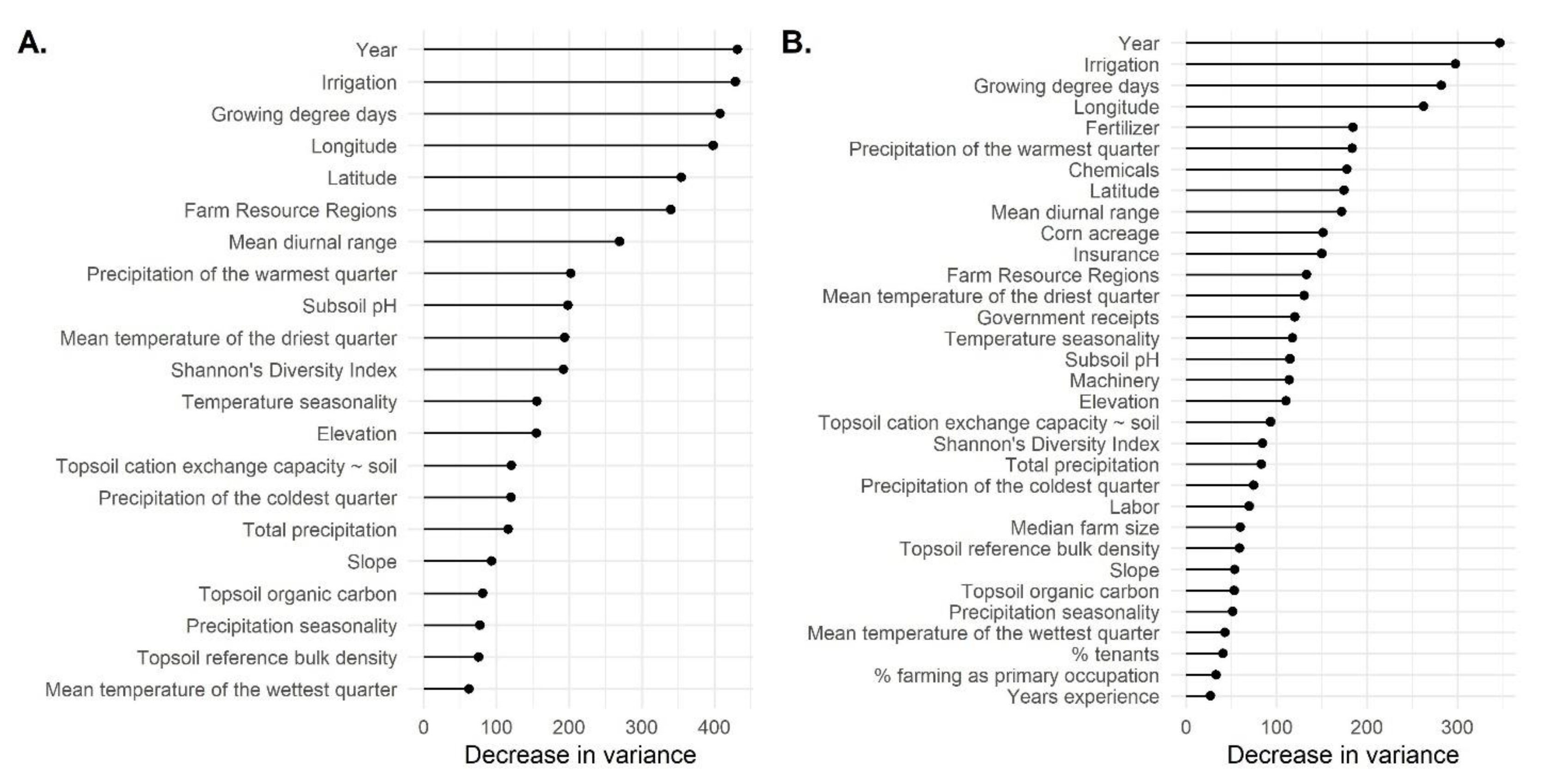
Permutation variable importance measures of the biophysical models (Figure 2A) revealed that that year was the most influential variable, followed by the percent irrigated agricultural acres, growing degree days, longitude and latitude, and Farm Resource Region. The remaining 15 climate, soil, land use, and topographic variables ranked lower in their relative importance. Variable importance measures of the farm(er) models (Figure 2B) revealed that that year was the most influential, followed by the percent irrigated agricultural acres, growing degree days, longitude, fertilizer applied, precipitation of the warmest quarter, chemicals applied, and latitude. The remaining 24 climate, soil, land use, topographic, and farm(er) variables ranked lower in their relative importance.

3.2. Group Exclusion, Predictive Accuracy, and Variable Importance

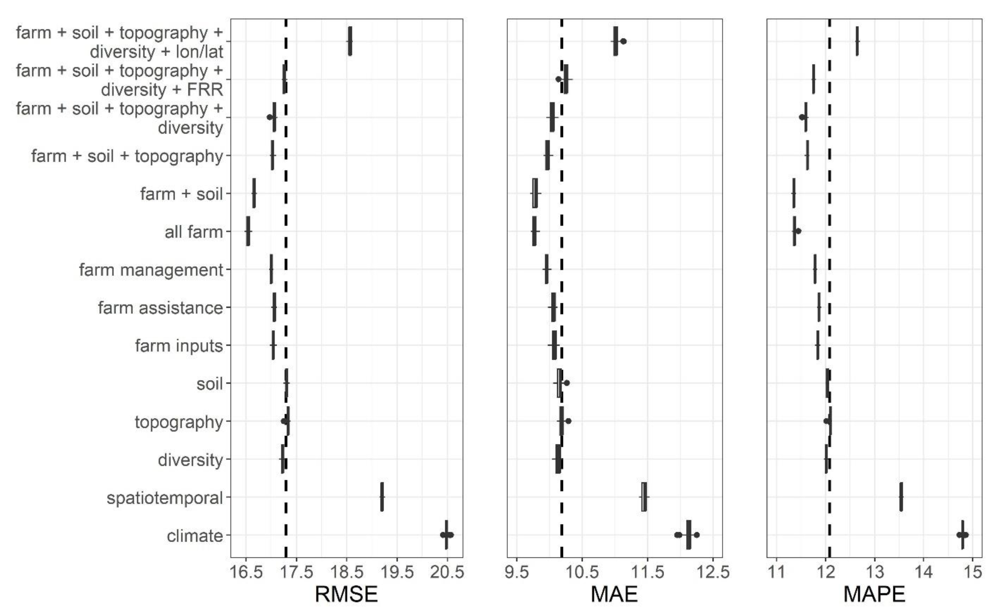
Figure 3 shows summaries of 5-fold cross validation for various combinations of input variables. Values on the y-axis indicate which groups of variables were removed for the model training. Error measures to the right (left) of the dashed line indicate a degradation (improvement) in model performance when the variables were removed. The results are somewhat surprising in that, despite variable importance measures that indicated important variables in each group (Figure 2A,B), the only groups that matter for prediction accuracy are the spatiotemporal and climate variables. Within the spatiotemporal variables, it is also shown that latitude and longitude have more influence on the accuracy results than the FRR designation. Further, the exclusion of farmer characteristics and soil information, both of which are intuitively related to yields, noticeably improves the performance of the model.
It is important to note that predictive accuracy does not imply causal inference for any of these variables. The high correlations observed between many of the explanatory variables make it impossible to infer causation in a model like this. However, the encouraging result is that corn yields can be imputed with relatively high accuracy using relatively few variables that are easy to collect.
The results also raise questions regarding the possible contradiction between the accuracy and variable importance measures. Permutation variable importance measures in RF models involve “scrambling” the information in a model variable and measuring the resulting loss in performance. This approach tends to associate importance with variables that are used both early and often in the creation of the individual regression trees that comprise the forest. Note that regression trees are grown by selecting the one split that minimizes the RMSE at each iteration. What is not clear in such a greedy algorithm is the potential quality of the “second place” variable that could have been used in the absence of first place for the splitting. In this context, we see that variables that are consistently used in the regression tree, and thus deemed important in the variable importance measures, apparently have “second place” variables that do near equally well in making model predictions, as indicated by the fact that removing these important variables does not compromise predictive performance. Indeed, the results outlined in this paper highlight the need for further scrutiny and additional approaches for evaluating variable importance in machine learning approaches.

3.3. RF Results Including Only Spatiotemporal and Climate Variables

After excluding all variable groups that do not contribute to prediction accuracy (Figure 3), our final model included only climate and spatiotemporal (year, latitude, and longitude) covariates. RF predictions were satisfactory, improving prediction accuracy by over 25% compared to naive imputation (infilling with median county yield across years, RMSE = 25.6–25.9 bushels/acre), with an RMSE of 17.1 bushels/acre (1.16 tons/hectare). This lightweight model explained about 81% of the variance in corn yield across the study period, with relative agreement between predictions and observations (Figure S6B), and similar relative errors across counties with a differing number of observations (Figure S7). Again, average errors were normally distributed, with about 50% of county-year errors falling within ±10 bushels/acre (Figure S6A).
Permutation variable importance measures of the reduced model (Figure 4) revealed that longitude was the most influential variable, followed by growing degree days, latitude, year, and the percent irrigated agricultural acres. The remaining eight climate variables ranked lower in their relative importance.

3.4. US Corn Yield in Ensemble Predicted Infilled Dataset

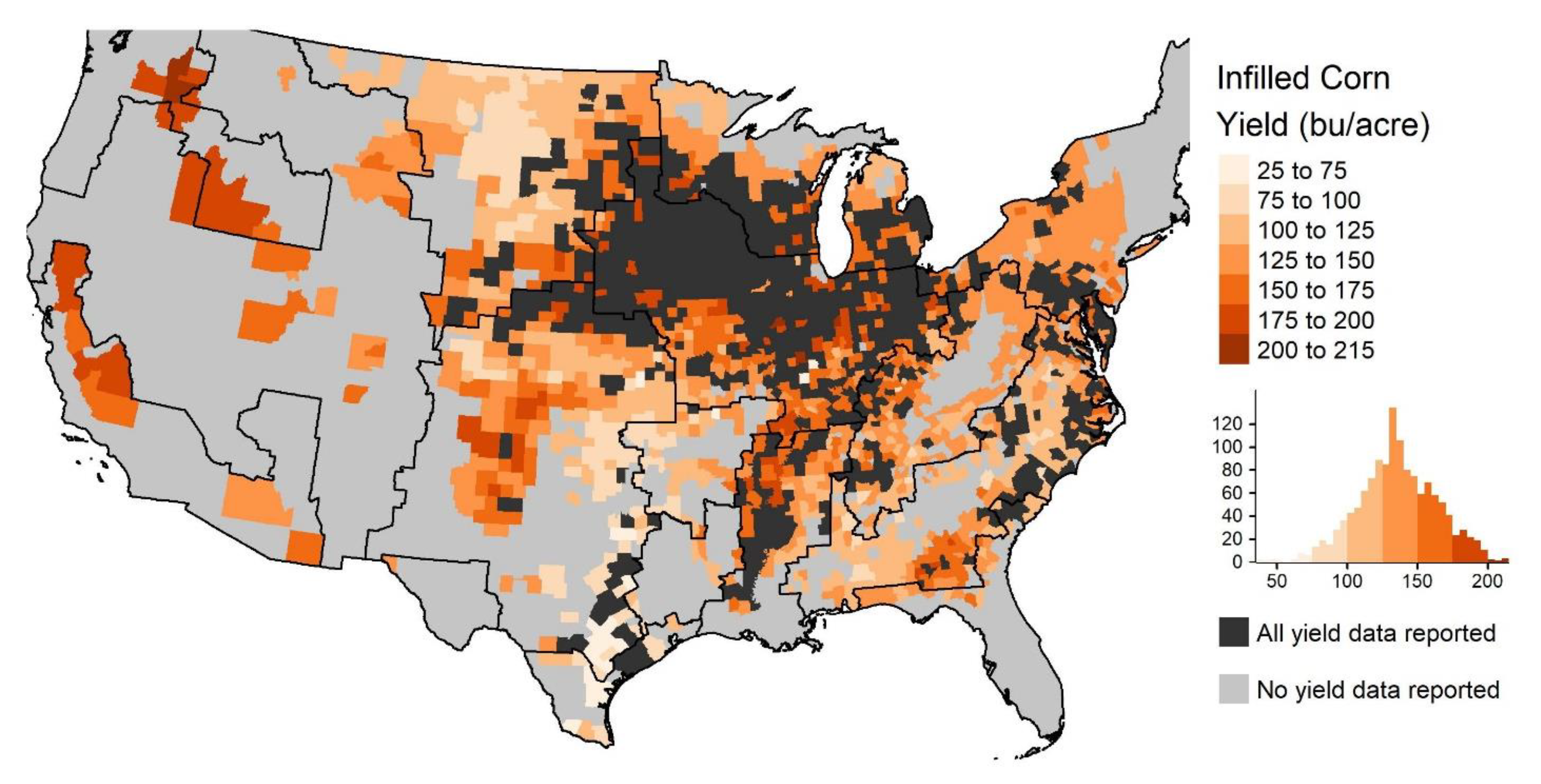
From the reduced ensembles, which are lightweight and still highly predictive, we built an infilled corn yield dataset, where each iteration of n = 50 RF models predicted county-year yields in each county reporting at least one year of production data. The reduced model predicted relatively low corn yields in the Northern Great Plains and Prairie Gateway regions, and relatively high yields in the Heartland and across the US West (Figure 5). We can think of this infilled data product as demonstrating yields farmers could have anticipated at the county-level had they grown corn in a particular year (for full documentation and year-by-year yield visualizations, see https://github.com/blschum/corn-yield-infill/blob/bean-collaboration/infill-dataproduct-documentation.Rmd).

3.5. Comparison to Other Methods

RF was intentionally selected due to its ease of use and high accuracy with very little hyperparameter tuning. That in mind, it is worthwhile to compare the possible improvements in accuracy that could come using other methods. For this, we use the stressor package [43], which is an R interface for the PyCaret package [44] in Python. The PyCaret packages provides low-code options for tuning and training a suite of machine learning models for use in accuracy comparisons. Because these benchmarks are not the focus of this paper, descriptions of the models are not provided in the text. Readers interested in model details can consult the documentation for Python’s scikit-learn package [45]. Table S6 provides the RMSE accuracy results for one iteration of the PyCaret package using all possible explanatory variables. Results are provided using a 75/25 training/test approach, along with the results for five-fold cross validation. Note that results vary slightly with each run due to the random nature of the data splitting, but the general differences in model performance are stable. The results show that RF is at or near the top of all considered machine learning methods. This speaks to RF’s ability to provide accurate results without much hyperparameter tuning, and reinforces its place as an accurate, yet accessible, approach for modeling agricultural yields.

4. Discussion

Our results demonstrate the effectiveness of RF regression in predicting corn yields across space and through time. Our reduced models had an RMSE of 17.1 bushels/acre (1.15 tons/hectare), comparable to the model performance in Jeong et al. (2016) [8] that made RF predictions on 30-year US corn yields, with an RMSE of 1.13 tons/hectare. These results provide confidence that we can derive reasonable yield estimates at the county-scale using publicly available data, reproducible methods, and a highly lightweight RF model, even in counties where corn yield has been minimally reported (n = 1 year). Our application of RF to corn yields led to four major findings: (1) the importance of time and space; (2) the importance of irrigation; (3) the importance of seasonal climate and bioclimatic indicators; and (4) the discrepancies between permutation variable importance measures and true contributions to model accuracy.
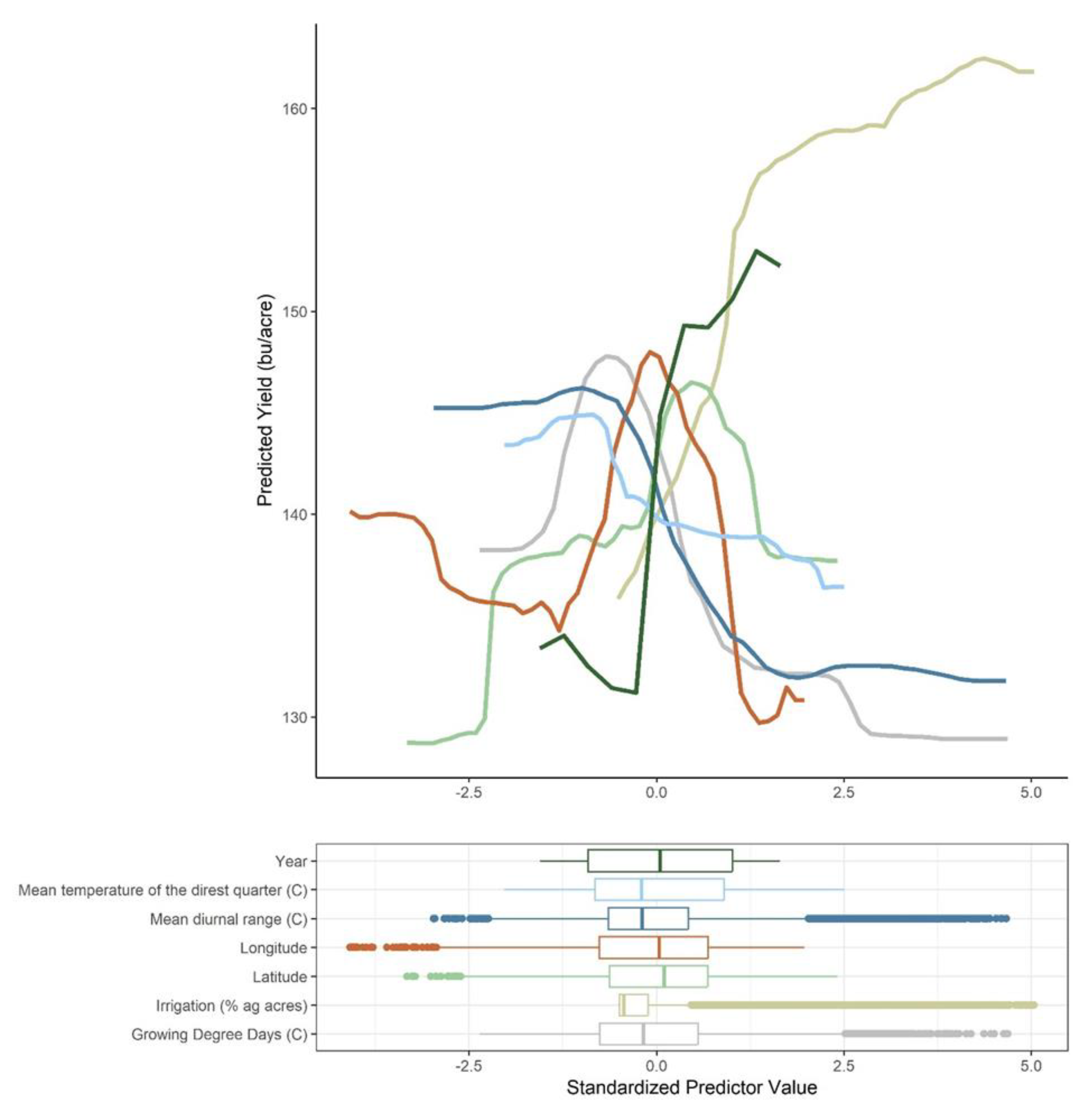
The first major finding is the persistent importance of temporal and spatial features to model performance and predictive capabilities in the RF models tested. Across all models, year remains consistently in the top five most important variables for prediction. Year soaks up major changes in technology, markets, management, and policies that affect corn production across the US. Recent work suggests that there are significant, positive, and increasing effects of time on corn yields in the coterminous US, effects that are comparable in magnitude to seasonal weather effects [10]. We see similar patterns suggested in our partial dependence plot on year, suggesting that yield growth in corn is indeed time dependent (Figure 6 and Figure S10m). Similarly, our indicators of space, longitude, and latitude, are consistently important across all models. These covariates soak up spatial variability at the county-level; we cannot account for and make decent replacements for covariates that do explain spatial variability. For instance, FRRs have different inherent biophysical suitability for growing corn, with some (e.g., in the Heartland, Mississippi Portal) having higher average regional yields than others (e.g., Northern Great Plains). Excluding FRR from our models, however, improves model accuracy while reducing model complexity, a win-win. Importantly, these time and space effects are outside a farmers’ scope of control—national-scale innovations and regional norms certainly shape a farmers’ baseline productivity (i.e., what is possible), but are not actionable features to be leveraged for productivity gains.
The second major finding is that the dominance of irrigated acreage on county agricultural lands contributes heavily to RF performance. Irrigation technologies transformed many agricultural systems in the US, allowing them to achieve higher yields than could be supported by the bioclimate and environment alone. This is true historically in the arid West and increasingly in the humid East, where farmers are capitalizing on irrigation technologies to ensure yields in harsh and changing climates [46]. Unsurprisingly, as irrigated acreage is increasing (growing in 59% of 1153 reporting counties between 2008 and 2018 across our panel dataset), irrigation withdrawals for agriculture in some areas are exceeding sustainable limits, depleting groundwater resources, reducing annual river discharge, and degrading ecosystem services to agriculture [47,48,49]. These cascading effects raise questions about how irrigation will continue to play a role in ensuring high levels of productivity in the future. The partial dependence plots from the reduced ensemble also suggest that the increasing dominance of irrigation is associated with diminishing returns to corn productivity after about 35% of a county’s agricultural lands are irrigated (Figure 6 and Figure S10B). At the same time, counties that are more difficult to predict (with errors > |10| bu/acre) tend to have a slightly greater irrigated presence on their agricultural lands (e.g., counties above the Ogallala Aquifer) (Figure S12); these findings warrant further exploration at sub-county scales and present interesting challenges to predicting yields into the future (i.e., how to accurately forecast future irrigation through space-time).
The third major finding, though unsurprising, is the importance of seasonal climate and bioclimatic indicators to yield prediction across all models. Mean diurnal range and growing degree days are consistently important predictors across RF models. The importance of climate and seasonal weather to agricultural yield is undeniable; in fact, other studies find that seasonal weather variability may explain up to 60% of yield variability in corn [50] and up to 70% in agricultural production more broadly [2]. The impacts of climate and weather on the agricultural sector are concerning considering the projected negative and uncertain effects of climate change and variability on US agriculture. Some projections suggest that by 2030, US corn production losses due to excess soil moisture and extreme precipitation events could double the loss levels in the early 2000s [51]. Others suggest that US corn yields could decline by between 43% and 79% (depending on the warming scenario) by the end of the century [14]. This would fundamentally alter the provisioning of food in the US and highlights the need to understand and predict the impacts of climate and weather events on yield. Our results demonstrate both the importance of precipitation and temperature to yield and the highly nonlinear relationships between weather and yield [14,52]. For instance, according to our partial dependence plots, yield increases up to a threshold of about 1700 GDDs and a mean diurnal range of about 11 °C; yield then decreases precipitously (Figure 6 and Figure S10a,e). In contrast is the relationship between yield and precipitation of the warmest quarter, where yield decreases below 100 mm precipitation, increases between 100 and 400 mm, and then stagnates above 400 mm (Figure S10i). These highly nonlinear relationships make clear why exploring models beyond traditional linear, parametric methods is key to understanding these complex relationships. These nonlinearities, in addition to the inherent spatial structure of seasonal weather and bioclimatic indicators ignored in RF, again reinforce the need for alternatives to traditional approaches in agricultural yield modeling.
The fourth and final major finding is the discrepancy we explored between permutation variable importance measures in our biophysical and farm(er) models and the true contributions to model accuracy of specific groups of variables (Figure 3). These results are surprising, despite variable importance measures that indicate important variables in each group (Figure 2A,B), with the only groups of variables required to preserve prediction accuracy being the spatiotemporal and climate variables. This finding makes for a far more lightweight model for infilling, which will allow for future researchers to build upon this project with relatively little data munging—a win for reproducibility and data science. But it also raises the question: What do we miss when we take variable importance as truth? In our case, we would have relied on a far more complicated model that provided few gains in accuracy for infilling; in others, the consequences may be broader, or more disruptive (e.g., suggesting paths forward for future research where paths do not exist).
We are not suggesting that the covariates identified as important using RF permutation variable importance measures are not. The results of our study only identify the variables needed for accurate prediction and do not identify causal links between covariates and crop productivity. We know, for instance, that crop and landscape diversity have been linked with enhanced ecosystem services to agriculture [53,54,55], and that increasing crop species diversity at the landscape scale may have significant benefits to corn yield [30]. We see a different trend reflected in our partial dependence plots of SDI on yield (Figures S8A and S9j), one that reflects our understanding of where corn yields are high: in places that maintain some of the least crop species diversity (e.g., the Heartland, Figure S11). We know, too, that biophysical suitability is managed for and altered by human activity [56], and that the strategies farmers employ impact agricultural productivity [57]. Despite this knowledge, many previous studies utilizing machine learning to predict crop yields have not included farm(er) data. These data may not have been included due to difficulties arising from data limitations, cleaning requirements, and imputation, or due to researchers discovering, as we have, that these characteristics do not meaningfully contribute to prediction accuracy at the county-level scale. Our domain knowledge about on-farm management’s direct impact on yields (e.g., [58,59]) refutes our findings and justifies exploration of the redistribution of variable importance in models that include farm(er) variables. Interestingly, the $/acre expenditure of fertilizer and chemicals on agricultural lands both exhibit saturating relationships with yield, where yield increases with up to USD $50/acre in chemicals, and USD $65/acre in fertilizer, and then remains near-constant as expenditures increase (Figures S8B and S9a,c), suggesting diminishing marginal returns to increased application. Government receipts and insurance payouts also exhibit similar saturating effects, where yield increases up to about USD $25/acre in government payments and USD $63/acre in insurance payouts and then levels off. These farm(er) characteristics clearly influence yield dynamics in highly nonlinear and important ways; their future inclusion in yield modeling is key to unlocking management strategies’ influence on agricultural yield. Building data that better measure farmer management strategies (e.g., fertilizer application, tillage, genomic choice) at the county-level will be essential to more accurately modeling agricultural yield in the future. Until these better data are built, however, as our study demonstrates, utilizing only biophysical features—and a reduced set of them at that—to model corn yield does produce quite accurate predictions.
RF is not, of course, without its shortfalls. We cannot explicitly account for spatial or temporal autocorrelation, for instance, and interpretation of model features is limited. Our models are also not without their limitations. For instance, it would be impossible for us to account for unpredictable time effects such as massive market shifts, policy overhauls, or environmental disasters. We hypothesize that model performance would improve with a larger training dataset, given RF’s data hungry nature (i.e., RF predictive performance improves with greater sample size), but also recognize that we may not be capturing large pieces of the agricultural puzzle that vary regionally (e.g., input use, management strategies). Given these limitations, and algorithmic promises, we suggest that our RF-built data product has the potential to: (1) help support, or otherwise oppose, the expansion of corn beyond its current cropscape; and (2) provide researchers with fodder for more nuanced and spatiotemporally coherent agricultural studies.
Our results demonstrate the efficacy and predictive capacity of a lightweight RF regression implementation in modeling complex corn yield responses over space and time to a small set of biophysical conditions (see full data product at https://github.com/blschum/corn-yield-infill/tree/bean-collaboration/results/ranger-infill/reduced). We make a distinct contribution by including farm(er) attributes, questioning and testing the “importance” of model variables, and building an infilled yield dataset. Given the sparse nature of current yield information, and the importance of agricultural yield to farmer livelihoods and to the US economy, we stand to benefit from a more complete representation of US agricultural yields. We argue that RF provides a useful, lightweight, and easy-to-implement tool for building this product.

5. Conclusions

The purpose of this study was to evaluate the spatiotemporal efficacy of RF in predicting corn yields. Results suggest that RF predicts US corn yields well across space and time by modeling the highly non-linear and interactive relationships that yield shared with irrigation, climate, space, and time. Importantly, our results build a case for questioning our interpretation of permutation importance in machine learning approaches to modeling when the explanatory variables are highly correlated with each other. Importance measures are often relied on by researchers to explain what matters in predicting a given outcome (e.g., yield), but our results suggest that the variables identified using RF as important may not be crucial to preserve accurate predictions. This highlights a broader issue of what makes a variable “important” in a machine learning context. As we have shown in this paper, the permutation-based variable importance approaches quantify how much a model uses a variable in prediction but fails to quantify the actual loss of accuracy that occurs in the absence of that variable. Further, our results provide a practical template for assessing variable importance in groups of data from the same source. For machine learning models where variable selection is not necessary for model building, it makes more sense, as we have shown in this paper, to consider the “value added” by considering the inclusion or exclusion of all variables from a common data source.
These results provide us with reasonable confidence in our infilled data product that utilizes RF’s characterization of spatiotemporal and climate covariates’ relationship to corn yield to predict yields in county-years with no reported yield data, producing a comprehensive corn yield dataset for the coterminous US. By infilling data, we can better understand agricultural yield in counties that have historically cultivated corn and better predict counties that may become corn producers as the climate changes. At the same time, our results point to the need for further work elucidating the contradictions that may arise in importance and accuracy measures. Infilled products using openly available covariates and easy-to-use, agile modeling approaches should aid policymakers, researchers, and land managers in adapting to and mitigating impacts of climate change on food, feed, fiber, and fuel production. Further, improved yield projections across space and time will allow for superior socioeconomic models and policies to support the expansion or contraction of corn production in current and future US cropscapes.
Though the literature is growing [17,19], machine learning techniques remain understudied in the field of crop yield modeling, especially at the US county-scale [20] in their inclusion of farm(er) predictors. Their superior performance in predicting agricultural yields suggests that their use warrants further exploration. Additional research is needed to build an ensemble of ensembles, each with their own strengths and weaknesses, and to develop more nuanced theoretical justification for model variable selection. This particular exploration helps us consider the extent to which publicly available and readily accessible data can be used to think about yield-driven questions in agriculture. The empirical evidence detailed in this paper provides a framework for future work linking crop yield and future cropscapes.

Supplementary Materials

The following supporting information can be downloaded at: https://www.mdpi.com/article/10.3390/agriculture13030618/s1, Figure S1: Count of missingness across CoA years; Figure S2: Correlation matrix for continuous predictors and corn yield; Figure S3: Map of counties excluded due to missing data across census years; Figure S4: Biophysical RF ensemble model performance based on five-fold cross validation; Figure S5: Farm(er) RF ensemble model performance based on five-fold cross validation; Figure S6: Group exclusion (climate + space + time) RF ensemble model performance based on five-fold cross validation; Figure S7: Boxplots of absolute percentage errors (APE) via 5-fold cross validation (one iteration) for all counties as organized by number of missing years; Figure S8: Partial dependence plots for consistently important variables in the (a) biophysical ensemble and (b) farm(er) ensemble; Figure S9: Partial dependence plots of important variables from biophysical and farm(er) ensembles (raw data, not standardized); Figure S10: Partial dependence plots of important variables from the reduced ensemble (raw data, not standardized); Figure S11: Bivariate choropleth constructed by binning county-level average corn yield (bushels/acre) and percent acres cultivated in corn on agricultural lands into thirds; each tercile is then paired and binned into distinct categories; Figure S12: Percent irrigated acreage on agricultural lands across study years (2008–2018) faceted by prediction class; Table S1: Full list of available historical biophysical predictors; Table S2: Average model performance; Table S3: RF variable importance rankings and accuracy metrics for biophysical models; Table S4: RF variable importance rankings and accuracy metrics for farm(er) models; Table S5: List of counties excluded due to missing data across census years, with Census FIPS codes. Table S6: The RMSE accuracy results for one iteration of PyCaret package using all possible explanatory variables. Results are provided using a 75/25 training/test approach, along with the results for 5-fold cross validation.

Author Contributions

Conceptualization, B.L.S., E.K.B. and M.A.Y.; methodology, B.L.S. and B.B.; formal analysis, B.L.S. and B.B.; data curation, E.K.B. and B.L.S.; writing—original draft preparation, B.L.S. and B.B.; writing—review and editing, B.B., E.K.B. and M.A.Y.; visualization, B.L.S. and B.B.; funding acquisition, E.K.B. and M.A.Y. All authors have read and agreed to the published version of the manuscript.

Funding

This article was supported by the Utah Agricultural Experiment Station [UTA01422] and [UAES9655], and Utah State University’s Ecology Center [07339-1001]. Any opinions, findings, and conclusions or recommendations expressed in this material are those of the author(s) and do not necessarily reflect the views of Utah State University or Emory University.

Institutional Review Board Statement

Not applicable.

Data Availability Statement

All data, code, products, and visualizations analyzed and generated during this study can be accessed publicly at https://github.com/blschum/corn-yield-infill/.

Acknowledgments

This research work is the part of the master thesis of the corresponding author, Britta L. Schumacher. Many thanks to Kaitlyn Spangler for clear and functional code that built Figure S11. Thanks also to Samuel Haycock for help with the {stressor} package for the machine learning benchmarks in Table S6.

Conflicts of Interest

The authors declare no conflict of interest.

References

  1. Bigelow, D.P.; Borchers, A. Major Uses of Land in the United States, 2012; U.S. Department of Agriculture, Economic Research Service: Washington, DC, USA, 2017. [Google Scholar]
  2. Liang, X.Z.; Wu, Y.; Chambers, R.G.; Schmoldt, D.L.; Gao, W.; Liu, C.; Liu, Y.A.; Sun, C.; Kennedy, J.A. Determining Climate Effects on US Total Agricultural Productivity. Proc. Natl. Acad. Sci. USA 2017, 114, E2285–E2292. [Google Scholar] [CrossRef] [Green Version]
  3. Mueller, N.D.; Gerber, J.S.; Johnston, M.; Ray, D.K.; Ramankutty, N.; Foley, J.A. Closing Yield Gaps through Nutrient and Water Management. Nature 2012, 490, 254–257. [Google Scholar] [CrossRef] [PubMed]
  4. Burchfield, E.; Matthews-Pennanen, N.; Schoof, J.; Lant, C. Changing Yields in the Central United States under Climate and Technological Change. Clim. Chang. 2020, 159, 329–346. [Google Scholar] [CrossRef]
  5. Ray, D.K.; Ramankutty, N.; Mueller, N.D.; West, P.C.; Foley, J.A. Recent Patterns of Crop Yield Growth and Stagnation. Nat. Commun. 2012, 3, 1293. [Google Scholar] [CrossRef] [PubMed] [Green Version]
  6. Zhao, C.; Liu, B.; Piao, S.; Wang, X.; Lobell, D.B.; Huang, Y.; Huang, M.; Yao, Y.; Bassu, S.; Ciais, P.; et al. Temperature Increase Reduces Global Yields of Major Crops in Four Independent Estimates. Proc. Natl. Acad. Sci. USA 2017, 114, 9326–9331. [Google Scholar] [CrossRef] [Green Version]
  7. Moore, F.C.; Baldos, U.L.C.; Hertel, T. Economic Impacts of Climate Change on Agriculture: A Comparison of Process-Based and Statistical Yield Models. Environ. Res. Lett. 2017, 12, 065008. [Google Scholar] [CrossRef]
  8. Jeong, J.H.; Resop, J.P.; Mueller, N.D.; Fleisher, D.H.; Yun, K.; Butler, E.E.; Timlin, D.J.; Shim, K.M.; Gerber, J.S.; Reddy, V.R.; et al. Random Forests for Global and Regional Crop Yield Predictions. PLoS ONE 2016, 11, e0156571. [Google Scholar] [CrossRef] [Green Version]
  9. Rissing, A.; Burchfield, E.K.; Spangler, K.A.; Schumacher, B.L. Implications of U.S. agricultural data practices for sustainable food systems research. Nat. Food. 2023, accepted. [Google Scholar] [CrossRef]
  10. Burchfield, E.K.; Nelson, K.S. Agricultural Yield Geographies in the United States. Environ. Res. Lett. 2021, 16, 054051. [Google Scholar] [CrossRef]
  11. Estes, L.D.; Bradley, B.A.; Beukes, H.; Hole, D.G.; Lau, M.; Oppenheimer, M.G.; Schulze, R.; Tadross, M.A.; Turner, W.R. Comparing Mechanistic and Empirical Model Projections of Crop Suitability and Productivity: Implications for Ecological Forecasting. Glob. Ecol. Biogeogr. 2013, 22, 1007–1018. [Google Scholar] [CrossRef]
  12. Lobell, D.; Asseng, S. Comparing estimates of climate change impacts from process-based and statistical crop models. Environ. Res. Lett. 2017, 12, 015001. [Google Scholar] [CrossRef]
  13. Lobell, D.B.; Burke, M.B. On the use of statistical models to predict crop yield responses to climate change. Agric. For. Meteorol. 2010, 150, 1443–1452. [Google Scholar] [CrossRef]
  14. Schlenker, W.; Roberts, M.J. Nonlinear Temperature Effects Indicate Severe Damages to U.S. Crop Yields under Climate Change. Proc. Natl. Acad. Sci. USA 2009, 106, 15594–15598. [Google Scholar] [CrossRef] [Green Version]
  15. Landau, S.; Mitchell, R.A.C.; Barnett, V.; Colls, J.J.; Craigon, J.; Payne, R.W. A parsimonious, multiple-regression model of wheat yield response to environment. Agric. For. Meteorol. 2000, 101, 151–166. [Google Scholar] [CrossRef]
  16. Sheehy, J.E.; Mitchell, P.L.; Ferrer, A.B. Decline in rice grain yields with temperature: Models and correlations can give different estimates. Field Crops Res. 2006, 98, 151–156. [Google Scholar] [CrossRef]
  17. Bali, N.; Singla, A. Emerging Trends in Machine Learning to Predict Crop Yield and Study Its Influential Factors: A Survey. Arch. Comput. Methods Eng. 2022, 29, 95–112. [Google Scholar] [CrossRef]
  18. Liakos, K.G.; Busato, P.; Moshou, D.; Pearson, S.; Bochtis, D. Machine learning in agriculture: A review. Sensors 2018, 18, 2674. [Google Scholar] [CrossRef] [PubMed] [Green Version]
  19. van Klompenburg, T.; Kassahun, A.; Catal, C. Crop yield prediction using machine learning: A systematic literature review. Comput. Electron. Agric. 2020, 177, 105709. [Google Scholar] [CrossRef]
  20. Shahhosseini, M.; Hu, G.; Huber, I.; Archontoulis, S.V. Coupling Machine Learning and Crop Modeling Improves Crop Yield Prediction in the US Corn Belt. Sci. Rep. 2021, 11, 1–15. [Google Scholar] [CrossRef]
  21. USDA ERS. Farm Resource Regions. Agricultural Information Bulletin 760, Washington, DC: USDA Economic Research Service, 2000. Available online: https://www.ers.usda.gov/webdocs/publications/42298/32489_aib-760_002.pdf?v=42487 (accessed on 1 June 2022).
  22. PRISM Climate Group. Oregon State University, 2014. Available online: https://prism.oregonstate.edu (accessed on 1 June 2020).
  23. Cross, H.Z.; Zuber, M.S. Prediction of Flowering Dates in Maize Based on Different Methods of Estimating Thermal Units. Agron. J. 1972, 64, 351. [Google Scholar] [CrossRef]
  24. Thornton, M.M.; Shrestha, R.; Wei, Y.; Thornton, P.E.; Kao, S.-C.; Wilson, B.E. Daymet: Monthly Climate Summaries on a 1-km Grid for North America, Version 4 R1; ORNL DAAC: Oak Ridge, TN, USA, 2022. [Google Scholar] [CrossRef]
  25. USDA-NASS. 2017 Census of Agriculture: United States Summary and State Data. Volume 1, Geographic Area Series, Part 51, AC-17-A-51, 2019. Available online: https://www.nass.usda.gov/Publications/AgCensus/2017 (accessed on 1 June 2022).
  26. USDA-NASS. QuickStats Database. Available online: https://quickstats.nass.usda.gov/ (accessed on 1 June 2020).
  27. Pervez, M.S.; Brown, J.F. Mapping Irrigated Lands at 250-m Scale by Merging MODIS Data and National Agricultural Statistics. Remote Sens. 2010, 2, 2388–2412. [Google Scholar] [CrossRef] [Green Version]
  28. Wieder, W.R.; Boehnert, J.; Bonan, G.B.; Langseth, M. Regridded Harmonized World Soil Database v1.2.; ORNL DAAC: Oak Ridge, TN, USA, 2012. [Google Scholar] [CrossRef]
  29. USDA-NASS. USDA National Agricultural Statistics Service (NASS) Cropland Data Layer Published Crop-Specific Data Layer. Available online: https://nassgeodata.gmu.edu/CropScape/ (accessed on 1 June 2020).
  30. Burchfield, E.K.; Nelson, K.S.; Spangler, K. The Impact of Agricultural Landscape Diversification on U.S. Crop Production. Agric. Ecosyst. Environ. 2019, 285, 106615. [Google Scholar] [CrossRef]
  31. Meyer, H.; Reudenbach, C.; Wöllauer, S.; Nauss, T. Importance of spatial predictor variable selection in machine learning applications—Moving from data reproduction to spatial prediction. Ecol. Modell. 2019, 411, 108815. [Google Scholar] [CrossRef] [Green Version]
  32. Breiman, L. Random Forests. Mach. Learn. 2001, 45, 5–32. [Google Scholar] [CrossRef] [Green Version]
  33. Biau, G.; Scornet, E. A Random Forest Guided Tour. Test 2016, 25, 197–227. [Google Scholar] [CrossRef] [Green Version]
  34. FAO/IIASA/ISRIC/ISS-CAS/JRC. Harmonized World Soil Database; Version 1.1; FAO: Rome, Italy; IIASA: Laxenburg, Austria, 2009; Available online: https://www.fao.org/3/aq361e/aq361e.pdf (accessed on 1 June 2020).
  35. Wright, M.N.; Wager, S.; Probst, P. Package ‘Ranger’, 2022. Available online: https://cran.r-project.org/web/packages/ranger/ranger.pdf (accessed on 1 June 2021).
  36. R Core Team. R: A Language and Environment for Statistical Computing. R Foundation for Statistical Computing, Vienna, Austria, 2022. Available online: https://www.R-project.org/ (accessed on 1 June 2020).
  37. Cutler, D.R.; Edwards Thomas, C.J.; Beard, K.H.; Cutler, A.; Hess, K.T.; Gibson, J.; Lawler, J.J. Random Forests for Classification in Ecology. Ecology 2007, 88, 2783–2792. [Google Scholar] [CrossRef]
  38. Liaw, A.; Wiener, M. Classification and Regression by RandomForest. R News 2002, 2, 18–22. [Google Scholar]
  39. Grömping, U. Variable importance assessment in regression: Linear regression versus random forest. Am. Stat. 2009, 63, 308–319. [Google Scholar] [CrossRef]
  40. Probst, P.; Wright, M.N.; Boulesteix, A.L. Hyperparameters and Tuning Strategies for Random Forest. WIREs Data Min. Knowl. Discov. 2019, 9, e1301. [Google Scholar] [CrossRef] [Green Version]
  41. Hastie, T.; Tibshirani, R.; Friedman, J.H.; Friedman, J.H. The Elements of Statistical Learning: Data Mining, Inference, and Prediction, 7th ed.; Springer: New York, NY, USA, 2017; pp. 181–184. [Google Scholar]
  42. Kutner, M.H.; Nachtsheim, C.J.; Neter, J.; Wasserman, W. Applied Linear Regression Models; McGraw-Hill/Irwin: New York, NY, USA, 2004; Volume 4, pp. 563–568. [Google Scholar]
  43. Haycock, S.; Bean, B. Stressor: Algorithms for Testing Models under Stress. 2023. Available online: https://github.com/beanb2/stressor (accessed on 22 January 2023).
  44. Ali, M. PyCaret: An Open Source, Low-Code Machine Learning Library in Python. 2020. Available online: https://www.pycaret.org (accessed on 22 January 2023).
  45. Pedregosa, F.; Varoquaux, G.; Gramfort, A.; Michel, V.; Thirion, B.; Grisel, O.; Blondel, M.; Prettenhofer, P.; Weiss, R.; Dubourg, V.; et al. Scikit-learn: Machine Learning in Python. J. Mach. Learn. Res. 2011, 12, 2825–2830. [Google Scholar]
  46. Troy, T.J.; Kipgen, C.; Pal, I. The Impact of Climate Extremes and Irrigation on US Crop Yields. Environ. Res. Lett. 2015, 10, 054013. [Google Scholar] [CrossRef] [Green Version]
  47. Perrone, D.; Jasechko, S. Deeper Well Drilling an Unsustainable Stopgap to Groundwater Depletion. Nat. Sustain. 2019, 2, 773–782. [Google Scholar] [CrossRef]
  48. Scanlon, B.R.; Faunt, C.C.; Longuevergne, L.; Reedy, R.C.; Alley, W.M.; McGuire, V.L.; McMahon, P.B. Groundwater Depletion and Sustainability of Irrigation in the US High Plains and Central Valley. Proc. Natl. Acad. Sci. USA 2012, 109, 9320–9325. [Google Scholar] [CrossRef] [Green Version]
  49. Smidt, S.J.; Haacker, E.M.K.; Kendall, A.D.; Deines, J.M.; Pei, L.; Cotterman, K.A.; Li, H.; Liu, X.; Basso, B.; Hyndman, D.W. Complex Water Management in Modern Agriculture: Trends in the Water-Energy-Food Nexus over the High Plains Aquifer. Sci. Total Environ. 2016, 566, 988–1001. [Google Scholar] [CrossRef] [Green Version]
  50. Ray, D.K.; Gerber, J.S.; Macdonald, G.K.; West, P.C. Climate Variation Explains a Third of Global Crop Yield Variability. Nat. Commun. 2015, 6, 5989. [Google Scholar] [CrossRef] [Green Version]
  51. Rosenzweig, C.; Tubiello, F.N.; Goldberg, R.; Mills, E.; Bloomfield, J. Increased crop damage in the US from excess precipitation under climate change. Glob. Environ. Chang. 2002, 12, 197–202. [Google Scholar] [CrossRef] [Green Version]
  52. Auffhammer, M.; Schlenker, W. Empirical Studies on Agricultural Impacts and Adaptation. Energy Econ. 2014, 46, 555–561. [Google Scholar] [CrossRef] [Green Version]
  53. Landis, D.A. Designing Agricultural Landscapes for Biodiversity-Based Ecosystem Services. Basic Appl. Ecol. 2017, 18, 1–12. [Google Scholar] [CrossRef] [Green Version]
  54. McDaniel, M.D.; Tiemann, L.K.; Grandy, A.S. Does Agricultural Crop Diversity Enhance Soil Microbial Biomass And. Ecol. Appl. 2014, 24, 560–570. [Google Scholar] [CrossRef] [Green Version]
  55. Tscharntke, T.; Klein, A.M.; Kruess, A.; Steffan-Dewenter, I.; Thies, C. Landscape Perspectives on Agricultural Intensification and Biodiversity—Ecosystem Service Management. Ecol. Lett. 2005, 8, 857–874. [Google Scholar] [CrossRef]
  56. Burchfield, E.K. Shifting Cultivation Geographies in the Central and Eastern US. Environ. Res. Lett. 2022, 17, 054049. [Google Scholar] [CrossRef]
  57. Hatfield, J.L.; Walthall, C.L. Meeting Global Food Needs: Realizing the Potential via Genetics × Environment × Management Interactions. Agron. J. 2015, 107, 1215–1226. [Google Scholar] [CrossRef] [Green Version]
  58. Grassini, P.; Thorburn, J.; Burr, C.; Cassman, K.G. High-yield irrigated maize in the Western U.S. Corn Belt: I. On-farm yield, yield potential, and impact of agronomic practices. Field Crops Res. 2011, 120, 142–150. [Google Scholar] [CrossRef] [Green Version]
  59. Kayad, A.; Sozzi, M.; Gatto, S.; Whelan, B.; Sartori, L.; Marinello, F. Ten years of corn yield dynamics at field scale under digital agriculture solutions: A case study from North Italy. Comput. Electron. Agric. 2021, 185, 106126. [Google Scholar] [CrossRef]
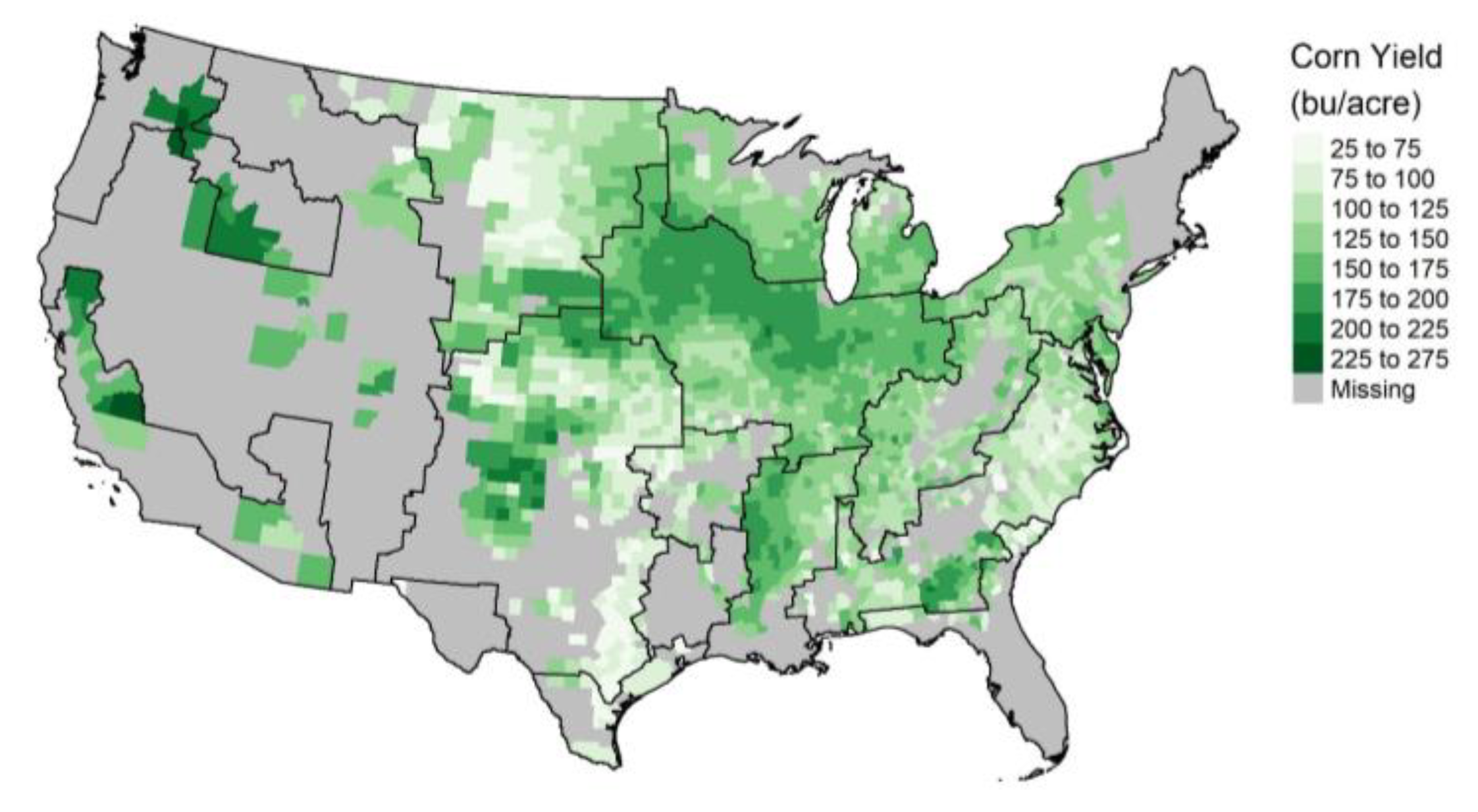
Figure 1. Farm Resource Region (FRR) boundaries and average corn yield (bushels per acre) recorded in USDA-NASS Surveys between 2008 and 2018; µpanel = 142.2 bushels/acre (9.56 tons/hectare), sdpanel = 39.4 bushels/acre (2.65 tons/hectare). FRRs as follows: (1) Heartland; (2) Northern Crescent; (3) Northern Great Plains; (4) Prairie Gateway; (5) Eastern Uplands; (6) Southern Seaboard; (7) Fruitful Rim; (8) Basin and Range; and (9) Mississippi Portal. The “missing” category refers to all counties where NASS reported no corn yields from 2008–2018.
Agriculture 13 00618 g001
Figure 2. Permutation variable importance for the (A) biophysical and (B) farmer RF resubstitution models of corn yield. The covariates appear on the y-axis and their contribution to decreased variance on the x-axis. Variables are listed in order of importance, with the most important variable being year and least important being mean temperature of the wettest quarter in panel (A), and years of experience in panel (B); see Table S1 for variable names, units, and descriptions.
Agriculture 13 00618 g002
Figure 3. Comparison of change in the 5-fold cross validation accuracy when variable groups are removed from the model. The dashed line represents the median accuracy metric for the model including all variables. The boxplots represent the range of errors observed in 50 replications of cross validation. Error metrics include the root mean square error (RMSE), the median absolute error (MAE), and the mean absolute percentage error (MAPE).
Agriculture 13 00618 g003
Figure 4. Permutation variable importance for the reduced resubstitution models of corn yield. The covariates appear on the y-axis and their contribution to decreased variance on the x-axis. Variables are listed in order of importance, with the most important variable being longitude and least important being mean temperature of the wettest quarter; see Table S1 for variable names, units, and descriptions.
Agriculture 13 00618 g004
Figure 5. Average corn yield in predicted infilled dataset in the reduced ensembles. Note: 1048 counties in light gray, are counties where n = 0 years of reported yield and were excluded from the infilling process, as per Figure 1, above. The remaining 745 counties marked in dark gray are those in which no infilling was necessary (e.g., in the Corn Belt, where NASS reports corn yield data each year).
Agriculture 13 00618 g005
Figure 6. Partial dependence plots for important variables in the reduced ensemble. Partial dependence is the dependence of the outcome on one predictor after averaging out the effects of all other predictors in the model [37]. Partial dependence plots graphically characterize the relationship between an individual predictor and the predicted values of yield. Data are visualized on a standardized scale i . e . , z μ z σ z to visualize all important covariates together. See Figure S10a–m for unstandardized relationships and all model covariates.
Agriculture 13 00618 g006
Disclaimer/Publisher’s Note: The statements, opinions and data contained in all publications are solely those of the individual author(s) and contributor(s) and not of MDPI and/or the editor(s). MDPI and/or the editor(s) disclaim responsibility for any injury to people or property resulting from any ideas, methods, instructions or products referred to in the content.