Non-Destructive Detection of Chicken Freshness Based on Electronic Nose Technology and Transfer Learning

Abstract

As a non-destructive detection method, an electronic nose can be used to assess the freshness of meats by collecting and analyzing their odor information. Deep learning can automatically extract features and uncover potential patterns in data, minimizing the influence of subjective factors such as selecting features artificially. A transfer-learning-based model was proposed for the electronic nose to detect the freshness of chicken breasts in this study. First, a 3D-printed electronic nose system is used to collect the odor data from chicken breast samples stored at 4 °C for 1–7 d. Then, three conversion to images methods are used to feed the recorded time series data into the convolutional neural network. Finally, the pre-trained AlexNet, GoogLeNet, and ResNet models are retrained in the last three layers while being compared to classic machine learning methods such as K Nearest Neighbors (KNN), Random Forest (RF), and Support Vector Machines (SVM). The final accuracy of ResNet is 99.70%, which is higher than the 94.33% correct rate of the popular machine learning model SVM. Therefore, the electronic nose combined with conversion to images shows great potential for using deep transfer learning methods for chicken freshness classification.

1. Introduction

Chicken is an important source of meat protein for humans, and consumer demand for chicken quality is increasing with the continuous improvement of living standards. Fresh chicken has a short shelf life, and consuming rotten or tainted meat might harm people’s health. A system that can rapidly assess the freshness of chicken can reduce potential food safety risks. The quality of meat can be represented by some indicators such as color, texture, pH value, tenderness, and freshness [1], with freshness being one of the most important indicators to evaluate the quality of chicken meat. An accurate, real-time, non-destructive detection and grading method for chicken freshness could better meet the market’s developing needs.

There have been two traditional methods for evaluating the freshness of chicken flesh: the first method is the combination of sensory evaluation and human experts [1]; another method is based on the physicochemical and microbiological analysis to determine pH, total volatile basic nitrogen (TVB-N), trimethylamine (TMA), and biogenic amines [2,3,4]. The first method is a time-consuming method due to the large amount of manual work required; the results of human evaluation could also be influenced by human emotions and health conditions [5]. The second method is destructive to the sample, and the process is complex and requires sophisticated instruments and professional domain knowledge [6]. Computer science-based meat freshness assessment techniques could help to alleviate some of the drawbacks mentioned above, such as making complicated judgments accurately and quickly [7]. However, they still cannot be deployed in the field due to the high cost and low efficiency [8,9,10,11,12,13]. Electronic nose technology has been applied to rapidly detect freshness due to its low cost and high efficiency [14,15]. Chemical compounds can be sensed and analyzed with the help of an electronic nose, which uses a simulated biological nasal anatomy and a specific sensor array. The gas data captured by the sensor array is processed and classified using machine learning methods. A demerit of this approach is that it necessitates feature extraction of the data. However, it is believed that feature extraction has limitations because it requires artificial selection of the extracted features, and the quality of the extracted features dramatically influences the quality of the final classification [16].

Deep learning has the advantage of being able to delve into deeper underlying laws and extract features automatically [17]. In recent years, deep learning-based classification methods have been applied to electronic nose technology to explore more efficient and effective solutions [16,18,19]. Nevertheless, how to achieve few-shot classification is also an issue that needs to be addressed because the learning process of deep networks is very complex and requires a large number of training samples. The sample collection of chicken requires a significant amount of time and workforce.

Transfer learning could be a viable solution to minor sample-based problems and is often deployed in agriculture-related applications [20,21]. However, few studies have discussed the issue of time series data processing based on the electronic nose. A method for classifying chicken freshness using the transfer learning approach was presented in this study. The original sensor response data is transformed into image data using three methods (scatter plot image, fitting curve image, and feature heat map). The last three layers of the convolution neural network, including the connected layer, SoftMax layer, and the classification output layer, are then replaced and retrained. At the same time, the former pre-trained layers in GoogLeNet, AlexNet, and ResNet models are retained to solve the chicken freshness classification problem using deep learning on small samples. Finally, the results based on the proposed model are compared to traditional machine learning models to assess the effectiveness of the proposed solution further.

2. Materials and Methods

2.1. Experimental Materials

The chicken samples used in this study were purchased in February 2022 from a local fresh poultry sale in Jiangbei New District, Nanjing. The test samples were taken from white feather chickens of the same breed slaughtered at the same time in a standard slaughter line to avoid the influence of the external humiture environment on meat quality during the slaughtering process. After slaughter, each sample was immediately removed from the breast portion of the chicken on both sides, cut evenly into equal portions, with a size of 3 cm × 3 cm × 1 cm [22], and transported to the laboratory within one hour in an insulated box, which was physically cooled using pre-chilled ice boxes to maintain the internal temperature at 4 °C. A total of 100 equal-sized experimental chicken breasts were obtained and stored in the incubator. They were then classified into three grades by numerical order, according to the chemical, texture profile, and qualitative analyses carried out by previous experts, with 1–3 d placement being classified as level 1, 4–5 d as level 2, and 6–7 d as level 3 [3].The grading criteria [23,24,25] are shown in

Table 1. Sensory grading scale for chicken.

Grade	External Quality	Internal Quality	Physical and Chemical Indicators
Level 1	The pieces are intact, free from defects, elastic, not sticky, with good skin adhesion, normal and even meat color, with the normal fresh chicken aroma	Myogenic fibers are in a relaxed state; the meat is tender and can be eaten normally.	pH value ≤ 6.0 TVB-N content ≤ 15 mg/100 g
Level 2	The pieces are relatively intact, generally elastic, slightly dry in appearance, with average flesh adhesion, dark and uneven color, and no particular odor	The chicken shrinks and becomes tough, with a slight loss of tenderness.	pH value > 6.5 TVB-N content 15~30 mg/100 g
Level 3	Pieces are fragmented, dark in color, dry, sticky, and smelly on the surface	Chicken is rotten inside and should not be eaten.	pH value > 6.7 TVB-N content > 30 mg/100 g

. The chicken was placed in a 4 °C thermostat for the number of days specified to record response data, and the corresponding level was used as the freshness label.

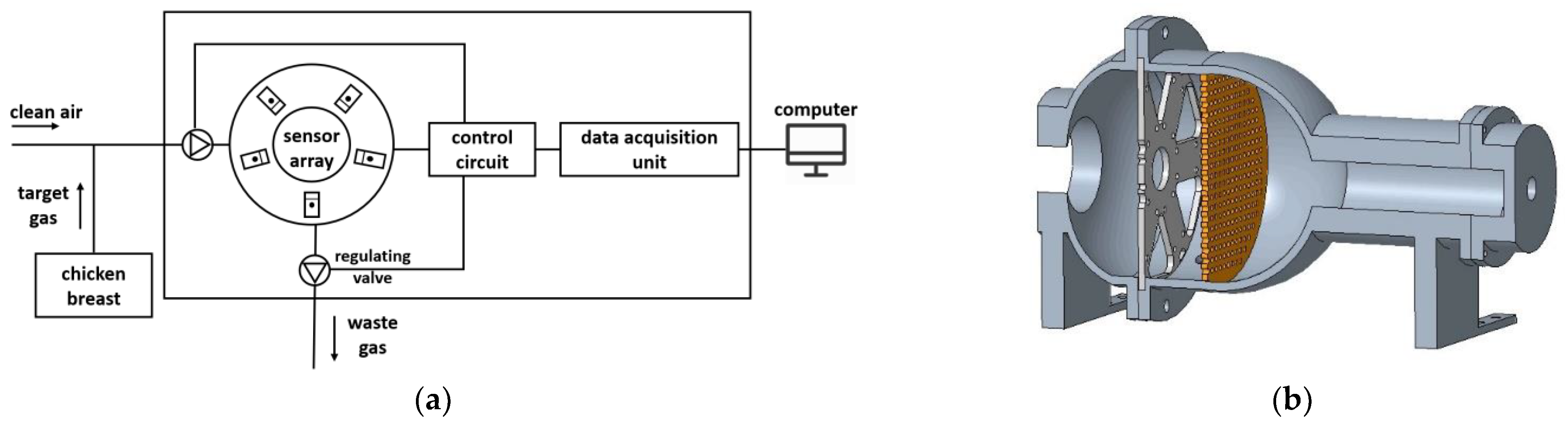
2.2. Electronic Nose Device and Collection of Odor Data

A self-developed electronic nose device was used in this study. Figure 1a shows the schematic diagram of the electronic nose system. The electronic nose system consists of a gas carrier bottle, gas piping, sensor arrays, control circuits, data acquisition units, gas control devices, such as regulating valves, and a computer. The nasal section is designed as a highly symmetrical circular tube with five built-in sensors. It contains a porous flow stabilizer to stabilize the transmitted airflow, as shown in Figure 1b. During the chicken’s storage and spoilage, various gases such as hydrogen sulfide, ammonia, and volatile organic compounds are volatilized [26,27]. According to the review, the MOS sensors initially selected for the device include TGS2600, TGS2602, TGS2620, and TGS822 from Figaro Japan and MQ135, MQ136, MQ137, and MQ138 from Zhengzhou Weisheng Company, etc. After initial comparison tests, five MOS sensors, including MQ135, MQ136, MQ137, MQ138, and TGS2602, are selected to form the sensor array, which have a fast response time and a large degree of response. The final sensor models and detection gases are shown in

Table 2. Sensor serial numbers and their detection gases.

Array Number	Detection of Gases	Model	Detection Range (‰)
Sensor 1	VOC, hydrogen sulfide, ammonia	TGS2602	0.001~0.030
Sensor 2	Hydrogen sulfide	MQ136	0.05~5.00
Sensor 3	Ammonia	MQ137	0.005~0.100
Sensor 4	Ammonia, hydrogen sulfide	MQ135	0.03~0.30
Sensor 5	Formaldehyde	MQ138	0.05~1.00

[28].

The operating temperature of the MOS sensor is around 300 °C. Before using the electronic nose device to collect gas data, the device must be preheated for 30 min. The sensors’ baseline stability affects the data quality baseline, so it is necessary to investigate the baseline stability of the sensor array. After the device has warmed up, the ES-3910 air pump and the regulating valve are switched on. The delivered dry, pure air at a constant rate of 15 L/min was then injected into the sample chamber to clean the sensor array. The response value of the sensors gradually stabilizes during the intake of air.

More than 20 measurements of the baseline response of each sensor have been made at different times of the year. It has been observed that the baseline fluctuations of the sensors are much smaller than their response to the target gas and do not interfere with the classification results.

Our team then collected gas data for the 300 samples in January 2022. The ambient room temperature was maintained at around 10 degrees Celsius. An air-drying tube was added to the transfer conduit connecting the sample chamber to the nasal cavity of the electronic nose to avoid the effect of high moisture from the chicken meat on the sensor response. For each experiment, the cut-up chicken meat was removed from the 4-degree Celsius thermostat, and the valve was adjusted to allow purified air to pass into the sample chamber. After about 5 s, the sample was placed in the sample chamber. Approximately 3 s later, the gas emitted from the chicken caused a rise in the sensor voltage value. The collection process lasts for 20 s. After the acquisition is completed and the sample is removed, the valve is adjusted, and standard air is passed in again to restore the sensor array and return the sensor response value to the baseline state. This purging process lasts for about 30 s. A total of 300 sets of electronic nose data were eventually obtained.

2.3. Computing Platforms

The software platforms used in this experiment are PyCharm 2021 (JetBrains, CZE) and Python 3.7 for machine learning algorithms and MATLAB 2020b for the neural network models.

The hardware in this study was an Intel^® Core i5-9300H CPU @ 2.40GHz, 8 G memory, and NVIDIA GeForce GTX 1650 graphics card.

2.4. Data Processing

2.4.1. Data Calibration

Following the above processes, the typical response curves recorded by the five sensors in the electronic nose are presented as a scatter plot in Figure 2.

The sensor response values were recorded at a 5 Hz sampling rate for approximately the first 20 s. To ensure the same size of data for each sample, the first 85 sample points were selected for each sensor data, i.e., a total of 85 × 5 sensors data points for each sample. Therefore, in the raw dataset, there were 300 sets of samples, that is, 100 sets in each freshness level.

As the response signal measured by the gas sensor can be affected by the external environment and produce a baseline drift, the raw data must first be corrected by Equation (1).

$$V_t=V-V_{base}$$

(1)

where V is the raw voltage data, V_base is the average value of the sensor response at pure air, and V_t is the corrected value. The raw data in the following descriptions are the calibrated voltage data.

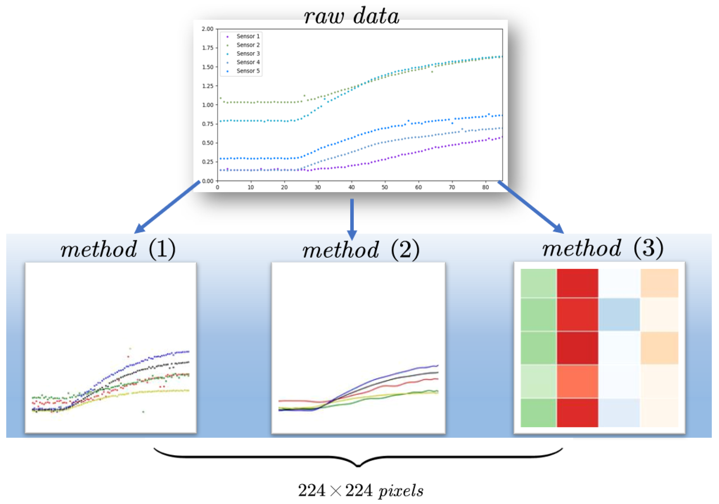
2.4.2. Input Images Preparation for Deep Learning Models

This subsection aims to convert the raw text dataset into an image dataset as the input of deep learning. Three ways are employed to transform the time series data into images that satisfy the 224 × 224 pixels image input form, which is required by deep learning models such as GoogLeNet and ResNet. These different basic ideas are raised below:

(1)

Transformation into image based on the raw discrete data;

(2)

Conversion to image based on fitted data;

(3)

Extraction of feature data from the fitted curve into image.

Based on the above ideas, the overall technical route is shown in Figure 3. It also shows the processing ideas of the machine learning methods as a comparison.

In this section, three methods are proposed to convert the electronic nose data into image data, the visual results of which are shown in Figure 4.

Method 1: Transformation of Raw Data into Input Images

Data matrix X, for a sample in the original data, is a two-dimensional sequence of the form m × n, where m is the length of the gas data and n is the number of sensors. In this study, the value of m is 85, and the value of n is 5. Matrix X can be expressed in Equation (2).

$$X={\left[\begin{array}{ccc}{x}_1^{t_0}& \cdots & x_5^{t_0}\\ \cdots & \cdots & \cdots \\ x_1^{t_0+84}& \cdots & x_5^{t_0+84}\end{array}\right]}_{85\times 5}$$

(2)

where the order of the columns represents the sensor number, and the order of the rows represents the corresponding sampling time.

The data distribution of the samples in each category X is shown in Figure 5. The distribution of data ranges varies considerably between the three categories of samples. The longitudinal range of the response value plot must be fixed in the final input image to maintain the relative positions of the curves and keep them consistent. This fixed range must clearly depict the trend of the response values for the different categories of samples simultaneously. A high range of longitudinal values for Level 1 and Level 2 chicken freshness samples will result in a compressed sample point distribution space. Setting a narrow longitudinal range will cause some of the sample points for Level 3 samples not to be displayed in their entirety in the image. The range of the longitudinal axis was set from −0.05 to 0.35, and the starting point of the longitudinal range was set to a negative value to prevent data points from being located at the edges. For the horizontal values, the maximum value is fixed at m, i.e., the horizontal range was set from 0 to 85.

To differentiate the response values of the individual sensors, each column of matrix X is configured to have the same color in the output image, and different colors are assigned for different columns.

After defining the range of horizontal and vertical values and the mapping colors corresponding to the sensor response values, the Matplotlib function in Python was used to fix the size of the generated image to 224 × 224 pixels to meet the needs of the input in the depth transfer model.

Method 2: Fitting the Curve to the Input Image

(1) Data pre-processing

The outliers in the raw data need to be removed before fitting the curve by setting a threshold at TH when the sensor response value, $V_i$, meets Equation (3).

$$|V_{i+1}-V_i|\&|V_i-V_{i-1}|>TH$$

(3)

where TH is defined by the mean of the absolute values of the differences between two adjacent points’ value in the rising phase. $TH=\frac{1}{60}{\displaystyle \sum _{i=1}^{60}|V_{i+1}-V_i|}$. The & symbol signifies that both equations satisfy the condition. For anomalous data, the treatment method substitutes the mean value of its two neighboring points with Equation (4).

$$V_i’=\frac{V_{i+1}+V_{i-1}}{2}$$

(4)

(2) Curve Fitting

After removing the outliers, the curve was fitted using a polynomial fit. The maximum number of fits was determined in the following way: the mean squared error (MSE) was calculated for the highest sub-terms of the fit at 20, 21, 22, 23, 24, and 25 by using Equation (5).

$$MSE=\frac{1}{n}{\displaystyle \sum _{i=1}^n{\left(Y_i-\widehat{Y}\right)}^2}$$

(5)

The highest power value corresponding to the lowest MSE is taken as the expression for the fitted curve. Sample fit effects are shown in Figure 6.

(3) The fitted curve is transformed into the input image

The method is similar to the steps used to transform the raw data into the input image, which is explained in Section 2.4.2, Method 1. The range parameters chosen in this step are the same as in Section 2.4.2, Method 1. Compared to Method 1, the image no longer contains anomalous data, and the sensor curve is smoother.

Method 3: Eigenvalue Mapping to Color Matrix Images

The third method differed from the previous two in the feature extraction phase. Before converting the raw data to an input image, features were extracted from part of the electronic nose data. A complete electronic nose response contains three phases: the baseline phase, the rising phase, and the recovery phase. However, the reaction between the target gas and the metal oxide semiconductor on the surface of the MOS sensor usually takes a long time to reach a stable value for data acquisition. By observing and analyzing the pre-experiment data before the formal experiments, we found that the main features of the sensor data for the different categories of samples are concentrated in the early phases of data acquisition. Thus, the first 17 s of data acquired by the electronic nose were used for subsequent feature engineering, significantly reducing the data acquisition time. In the first 17 s, only the baseline phase and part of the rising phase could be recorded, so only the response features from the recorded data could be extracted. Four features are selected: maximum response value, peak area, maximum first-order derivative, and maximum second-order derivative [29]. The four features are shown in Figure 7.

Once the feature matrix A has been extracted, it needs to be normalized to eliminate the effects of dimensionality. The normalization method chosen is maximum–minimum normalization, which is given by Equation (6).

$$a_{ij}\text{’}=\frac{a_{ij}-\underset{j}{min}{a}_{ij}}{\underset{j}{max}{a}_{ij}-\underset{j}{min}{a}_{ij}}$$

(6)

where i is the sensor number, j is the feature number, $a_{ij}$ is the result before normalization, and $a_{ij}’$ is the result after normalization.

Based on the above method, a total of 20 features can be extracted from each sample at 4 features × 5 sensors, with each feature value falling within the interval of [0,1]. The following procedure was used to turn the feature data into an image: In the first place, each feature’s color base was set, necessitating the four features to have separate color bases from one another. For the same type of feature, the feature value was set to be darker the closer it was to 1 and lighter the closer it was to 0. A blank image of 224 × 224 pixels was then divided into five equal parts vertically and four equal parts horizontally. Following the equal division, the colors corresponding to the 20 feature values of a sample were filled into the twenty squares, generating the final image data, as shown in Figure 8.

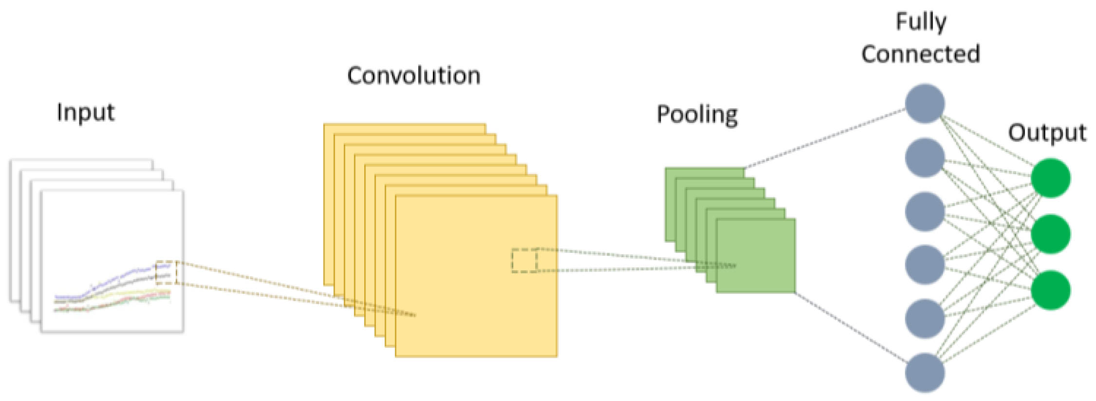
2.5. Deep Convolutional Neural Network Model Construction

As shown in Figure 9, the typical convolutional neural network (CNN) architecture consists of a convolutional layer, a pooling layer, and a fully connected layer. The convolutional layer’s main performance is extracting features from the image using kernels or filters. The pooling layer reduces overfitting by downsampling and compressing data and parameters. After several convolutional and pooling layers, the fully connected layer connects nodes in the previous layer and classifies them into different labeled categories. In this work, the three most used models in the agriculture of deep CNN, namely AlexNet, GoogLeNet, and ResNet50, are applied to classify chicken freshness. The AlexNet model uses dropout to solve the overfitting problem effectively and proposes a local response normalization layer to enhance the model’s generalization ability. In GoogLeNet, multi-scale feature fusion is achieved by optimizing the network structure and using convolutional kernels of different sizes. ResNet solves the problem of vanishing gradient and degradation in practical applications using residual connections. All these characteristics not only help to improve the accuracy but also reduce the computational time.

2.5.1. AlexNet

The AlexNet model [30] consists of five convolutional layers and three pooling layers, and three fully connected layers. The structure is very similar to the original convolutional network model, LeNet, except that AlexNet uses more convolutional layers and a wider parameter space. The network equivalent makes it possible to maximize the objective of the multi-categorical logistic regression model, using ReLu instead of the traditional Sigmoid and Tanh functions as non-linear activation functions for the neurons and proposing the Dropout method to mitigate the overfitting problem.

2.5.2. GoogLeNet

GoogLeNet is a neural network structure with only 22 layers of depth, which was used by Szegedy et al. [31] in 2014 at the 2014 Large Scale Vision Challenge (ILSVRC-2014). In this study, compared to models such as AlexNet and VGG, GoogLeNet compensates for the computational cost of building a deeper network by designing the Inception module.

The main idea of the Inception modules is to use convolutional kernels of different sizes to achieve different scales of perception so that multi-scale feature fusion can be achieved. GoogLeNet is composed of nine Inception modules, two convolutional layers, and three pooling layers. The structure is shown in Figure 10, where a 1 × 1 convolutional layer is added after the 3 × 3 pooling layer before the 3 × 3 and 5 × 5 convolutional layers to reduce the dimensionality [31].

2.5.3. ResNet50

The ResNet50 model [32] addresses the “degradation” of the network by using residual connections. Through experiments, the ResNet team found that the model’s accuracy increases and decreases as the layers of the network deepened, a phenomenon the team refers to as “degradation”. To address this problem, ResNet has proposed a residual learning framework that is easy to optimize and can improve performance as the depth of the network increases. The residual block can be performed by Equation (7).

$$x_{l+1}=\mathrm{Re}Lu\left(x_l+F\left(x_l,w_l\right)\right)$$

(7)

where $x_l$ and $x_{l+1}$ represent the input and output of the l and l + 1 residual blocks, respectively, F(x) is the residual function, and $w_l$ is the weight function of the residual block.

The residual learning module is shown in Figure 11. This study uses ResNet with a depth of 50 layers, which contains 48 convolutions, 1 average-pooling, and 1 max-pooling layer [32].

2.5.4. Transfer Learning

Training a deep CNN model of high accuracy requires a large dataset for improving its accuracy. For example, the championed models mentioned above were trained based on the ImageNet dataset, which contains over 14 million images. Such complete training involves a large amount of financial and computational resources. For the chicken freshness classification task, it is tough to meet these high-cost conditions. Luckily, this problem could be solved by transfer learning [33]. Transfer learning is based on the fact that the convolutional and pooling layers of those good deep networks gain the ability to extract features, which means they can be repurposed or transferred to another network when the target tasks are changed. Only the fully connected layer and the output layer contain some label information for classification. Therefore, this research downloads the CNN models mentioned above and integrates them with new models, with the aim of training the chicken flesh classification task with higher accuracy and shorter training time compared with CNN training from scratch.

The proposed model for the chicken freshness classification is based on importing the pre-trained weights in the initial set of layers and replacing the latter layers of each of the three architectures (AlexNet, GoogLeNet, and ResNet). As shown in Figure 12, the converted images will enter the frozen convolution layers and pooling layers for feature extraction then be classified in the last three layers (fully connected layers, SoftMax classifier layers, and classification layers). The number of neurons in the fully connected layers is all modified into three, representing that our new task has three classes instead of 1000 classes in the origin models. The bottom layers of the three origin and modified models are illustrated in Figure 13.

3. Results and Discussion

3.1. Experimental Setup

The 100 samples collected contain three classes of chicken freshness. Initially, all samples are randomly divided into the training and test sets at 7:3 training-to-test ratio. Each experiment is repeated ten times. For the traditional machine learning approach, the 20 original feature parameters extracted are subjected to principal component analysis to obtain 13 principal components (95% contribution) as model input, and three classes are used as labels; the machine learning model is then trained according to the corresponding set parameters. For the deep learning model, an initialized network parameter is set first, and this is adjusted when discussing the effect of different factors on the results. In contrast, the same initialized parameters mentioned above are used for the other parameters. The initial parameters set for machine learning and deep learning are shown in

Table 3. Initial parameters used for machine learning and deep transfer learning.

Classification Algorithms	Relevant Parameters
Support Vector Machines (SVM)	Penalty parameter c = 2.0; kernel: “RBF”;
Random Forest (RF)	Feature selection criterion: Gini Min_samples_split:5
K Nearest Neighbors (KNN)	K neighbors:5
GoogLeNet	Initial learning rate: 0.0001. MaxEpochs:3; MiniBatchSize:10; Optimization algorithm: SGDM
AlexNet
ResNet

.

3.2. Influence of the Input Pattern of the Deep Transfer Model

For the deep learning models, there are three ways to pre-process the raw data: Method 1 is to convert the scatter plot of the raw data into images, Method 2 is to convert the curve fitted plot into images, and Method 3 is to extract the features of the fitting curves and then convert them into the heatmap. Comparing the three input models, it can be seen that using different networks has a limited effect on Method 1 and Method 2. The best-performing ResNet in Method 1 only outperforms the other two models by 0.23% and 0.43%, while the best-performing AlexNet in Method 2 only outperforms the other two models by 0.67% and 0.3%. Thus, all three classical CNN networks perform well in these two Methods. This reflects the superiority of automatic feature extraction by deep learning. Because Method 2 adds a pre-processing step to remove anomalous data, the images have a smoother sensor response curve than the original scatter data and therefore have a higher classification accuracy.

For Method 3, the original data is mapped into the image data after feature extraction, making it more difficult for the CNN to find patterns in the extracted features. Therefore, there is a significant difference in the performance of the models trained by the first two Methods. In Method 3, ResNet performs better than the other two CNN algorithms. The correct rate of 96.67% was achieved, which compares favorably with the training results of the other two models. The results are shown in

Table 4. Correctness rate for different input modes.

Method	GoogLeNet	AlexNet	ResNet
Method 1	99.10%	98.90%	99.33%
Method 2	99.03%	99.70%	99.40%
Method 3	90.22%	92.91%	96.67%

, and the loss function corresponding to the best model performance for each Method is shown in Figure 14.

3.3. Comparison of Experimental Training Results

The classification results of three common machine learning algorithms (SVM, RF, and KNN) are used to compare with deep learning methods. First, the 20-dimensional features in Section 2.4.2, Method 3, were downscaled to 13 dimensions using PCA with a cumulative contribution of 95%. The data were fed into the model for training to obtain the final average correct rate and confusion matrix. Of the three machine learning methods, SVM achieved the highest classification accuracy (94.3%), as shown in

Table 5. Classification Accuracy of Machine learning.

Algorithms	SVM	RF	KNN
Accuracy	94.33%	94.01%	92.08%

and Figure 15. It can be seen from Figure 15 that machine learning models tend to make wrong verdicts when the true label is level 1 and level 2.

3.4. Effect of Training Set Size on Model Performance

The difference in the number of training samples largely determines the model’s performance. [34] All other things being equal, this section adjusts the ratio of the training and test sets for traditional machine learning algorithms and three CNN networks, and conducts three sets of experiments to divide the ratios of training and test sets as follows: 1:9, 2:8, 3:7, 4:6, 5:5, 6:4, 7:3, and 8:2. (i.e., the training sample sizes are 30, 60, 90, 120, 150, 180, 210, and 240.) As shown in Figure 16, the number of training samples increases (also stands for the proportion increases in each plot), and the correctness of the model increases accordingly. There is no significant difference between Method 1 and Method 2 for the different division ratios in the range of 180–240, while the percentage of the training set divided by Method 3 decreases, and the correctness rate decreases accordingly. The use of a 7:3 training-to-test ratio is a better choice for this study as the sample size is insufficient for a test set with too few divisions, which would also result in a poor reflection of the model’s accuracy.

3.5. Influence of Network Parameters

The hyperparameters used above were initialized uniformly based on the references. To discuss the effect of network parameters on the experimental results, this subsection looks at the training results by varying the learning rate and different optimization algorithms.

(1)

Effect of Batch Size on results

The size of the mini-batch is also an important parameter affecting the model’s accuracy. In this section, we have chosen 10, 16, 32, 64, and 128 as the batch sizes for evaluation in transformation Method 1, and the results are shown in Figure 17. The accuracy variation in the range of 10–64 of the mini-batch is controlled within 5%, with the highest accuracy of the model chosen to be 10 or 12. Therefore, increasing the batch size does not improve the model accuracy, while the accuracy drops significantly after increasing to 128. Based on the experimental results, choosing 10 as the mini-batch size allows the models to achieve better accuracy.

(2)

Effect of Batch Size on results

The learning rate determines the step size in each iteration so that the loss function converges to a minimum value. While the small learning rate leads to a slower convergence process, the large learning rate may directly cross the global optimum point. The learning rate settings of 0.001, 0.0001, and 0.0005 were chosen for comparison. As shown in

Table 6. Accuracy of the model at different learning rates.

	Learning Rate	0.001	0.0001	0.0005
GoogLeNet	Method 1	95.78%	99.10%	92.22%
	Method 2	98.89%	99.03%	96.44%
	Method 3	81.23%	90.22%	88.89%
AlexNet	Method 1	33.33%	98.90%	33.33%
	Method 2	33.33%	99.70%	33.33%
	Method 3	33.33%	92.91%	86.11%
ResNet	Method 1	97.56%	99.33%	98.89%
	Method 2	99.26%	99.40%	98.89%
	Method 3	94.78%	96.67%	96.67%

, we found that when the AlexNet learning rate was set to 0.001, the correct rate was 33.33% regardless of the method used, and this was also the case for Method 1 and Method 2, with a learning rate of 0.0005. Checking the corresponding loss function, it was found that the gradient vanished, and the value of the loss function became not a number (NaN) after around 28 iterations, as shown in Figure 18. The excessive learning rate caused the parameters to be updated too quickly, which made the model no longer valid. For GoogLeNet and ResNet, the difference in the effect of changing the learning rate of GoogLeNet on the model ranged from 0.15% to 8%. In contrast, the effect on ResNet was insignificant. However, a combined comparison of 0.0001 was still the best choice of learning rate.

(3)

Impact of different optimizers

Commonly used optimizers are SDGM (Stochastic Gradient Descent with Momentum), RMSProp (Root Mean Square Prop), and Adam (Adaptive moment estimation). Adam and RMSProp are generally faster, while SGDM gives better results. To investigate the impact of the different optimizers applied to this dataset, we selected the above three optimizers for training. The results are shown in

Table 7. Model accuracy using different optimizers.

	Optimizers	Adam	SDGM	0.0005
GoogLeNet	Method 1	91.33%	99.10%	76.22%
	Method 2	97.78%	99.03%	93.11%
	Method 3	62.67%	90.22%	45.78%
AlexNet	Method 1	98.33%	98.90%	98.44%
	Method 2	98.89%	99.70%	98.89%
	Method 3	93.33%	92.91%	84.89%
ResNet	Method 1	98.89%	99.33%	99.33%
	Method 2	99.56%	99.40%	99.56%
	Method 3	97.11%	96.67%	95.56%

, which shows that the results of the models trained with different optimizers vary significantly for different network structures. The difference between the results of AlexNet and ResNet networks when using Adam optimization and SDGM is not significant, and their classification accuracy is better than SDGM on Method3. In contrast, for GoogLeNet, the correct rate using Adam and RMSProp has a significant downward trend and is prone to gradient disappearance. Overall, for AlexNet and ResNet, the Adam and SDGM optimizers have better results. At the same time, GoogLeNet can only choose to use the SDGM optimization, and the other two methods have poor robustness of the trained models.

4. Conclusions

A self-designed electronic nose system was utilized to collect chicken flesh gas samples, and a deep transfer learning model was designed and implemented to classify the freshness of chicken in this research. The basic nasal structure was established and refined for the electronic nose part, incorporating a steady flow plate to increase airflow stability. In addition, to shorten the time to detect the gas, only the values of the baseline phase and part of the rising phase of the sensor data were recorded and used to extract the features for further analysis. A total of twenty features from the five sensors were transformed into images (Method 3) as input for deep learning and as comparison input for the classical machine learning classifier.

Concerning classification using deep learning, firstly, because the time series data acquired by the electronic nose sensor array cannot be used directly as input to the convolutional neural network, it must first be converted into picture data. Three methods were proposed to convert the sensor data matrix and compare the results of the three methods in this research. Secondly, considering the problem that manual collection of chicken sample data is time-consuming and labor-intensive, resulting in a small number of usable samples insufficient to train a CNN, transfer learning was proposed by inputting images into pre-trained networks AlexNet, GoogLeNet, and ResNet to fine-tune the models. Comparing typical machine learning models after several experiments on each network demonstrated that the deep transfer learning model has a classification accuracy of 99.7%., and the accuracy of applying the fitted data into images is the highest, followed by the original data and the feature matrix heat map. All three approaches outperformed the machine learning SVM model’s classification result of 94.33%, indicating that the proposed electronic nose chicken freshness assessment model has a better performance in identifying chicken freshness levels.

From the analysis of the experimental results, the reason why deep learning can achieve better classification results likely stems from its ability to extract features autonomously. When using machine learning to achieve classification, the researcher needs to artificially select the features and the number of features to be extracted. This requires the researcher’s experience and many trials to improve accuracy. Ultimately, the upper limit of accuracy of machine learning is affected by this factor. Deep learning is more effective in reducing this factor and has some promise for the classification of time-series data.

References

1. Li, H.; Chen, Q.; Zhao, J.; Wu, M. Nondestructive detection of total volatile basic nitrogen (TVB-N) content in pork meat by integrating hyperspectral imaging and colorimetric sensor combined with a nonlinear data fusion. LWT 2015, 63, 268–274. [Google Scholar] [CrossRef]
2. Rodtong, S.; Nawong, S.; Yongsawatdigul, J. Histamine accumulation and histamine-forming bacteria in Indian anchovy (Stolephorus indicus). Food Microbiol. 2005, 22, 475–482. [Google Scholar] [CrossRef]
3. Rukchon, C.; Nopwinyuwong, A.; Trevanich, S.; Jinkarn, T.; Suppakul, P. Development of a food spoilage indicator for monitoring freshness of skinless chicken breast. Talanta 2014, 130, 547–554. [Google Scholar] [CrossRef] [PubMed]
4. Khulal, U.; Zhao, J.; Hu, W.; Chen, Q. Intelligent evaluation of total volatile basic nitrogen (TVB-N) content in chicken meat by an improved multiple level data fusion model. Sens. Actuators B Chem. 2017, 238, 337–345. [Google Scholar] [CrossRef]
5. Korel, F.; Luzuriaga, D.; Balaban, M. Objective Quality Assessment of Raw Tilapia (Oreochromis niloticus) Fillets Using Electronic Nose and Machine Vision. J. Food Sci. 2001, 66, 1018–1024. [Google Scholar] [CrossRef]
6. Chen, Q.; Hui, Z.; Zhao, J.; Ouyang, Q. Evaluation of chicken freshness using a low-cost colorimetric sensor array with AdaBoost–OLDA classification algorithm. LWT 2014, 57, 502–507. [Google Scholar] [CrossRef]
7. Du, C.-J.; Sun, D.-W. Learning techniques used in computer vision for food quality evaluation: A review. J. Food Eng. 2006, 72, 39–55. [Google Scholar] [CrossRef]
8. Xiong, Z.; Sun, D.-W.; Pu, H.; Xie, A.; Han, Z.; Luo, M. Non-destructive prediction of thiobarbituricacid reactive substances (TBARS) value for freshness evaluation of chicken meat using hyperspectral imaging. Food Chem. 2015, 179, 175–181. [Google Scholar] [CrossRef]
9. Kandpal, L.M.; Lee, H.; Kim, M.S.; Mo, C.; Cho, B.-K. Hyperspectral Reflectance Imaging Technique for Visualization of Moisture Distribution in Cooked Chicken Breast. Sensors 2013, 13, 13289–13300. [Google Scholar] [CrossRef] [Green Version]
10. Xiong, Z.; Sun, D.-W.; Pu, H.; Gao, W.; Dai, Q. Applications of emerging imaging techniques for meat quality and safety detection and evaluation: A review. Crit. Rev. Food Sci. Nutr. 2017, 57, 755–768. [Google Scholar] [CrossRef]
11. Pérez-Palacios, T.; Antequera, T.; Durán, M.L.; Caro, A.; Rodríguez, P.G.; Palacios, R. MRI-based analysis of feeding background effect on fresh Iberian ham. Food Chem. 2011, 126, 1366–1372. [Google Scholar] [CrossRef]
12. Taheri-Garavand, A.; Fatahi, S.; Shahbazi, F.; De La Guardia, M. A nondestructive intelligent approach to real-time evaluation of chicken meat freshness based on computer vision technique. J. Food Process Eng. 2019, 42, e13039. [Google Scholar] [CrossRef]
13. Antequera, T.; Caballero, D.; Grassi, S.; Uttaro, B.; Perez-Palacios, T. Evaluation of fresh meat quality by Hyperspectral Imaging (HSI), Nuclear Magnetic Resonance (NMR) and Magnetic Resonance Imaging (MRI): A review. Meat Sci. 2021, 172, 108340. [Google Scholar] [CrossRef]
14. Tan, J.; Xu, J. Applications of electronic nose (e-nose) and electronic tongue (e-tongue) in food quality-related properties determination: A review. Artif. Intell. Agric. 2020, 4, 104–115. [Google Scholar] [CrossRef]
15. Shi, H.; Zhang, M.; Adhikari, B. Advances of electronic nose and its application in fresh foods: A review. Crit. Rev. Food Sci. Nutr. 2018, 58, 2700–2710. [Google Scholar] [CrossRef]
16. Wang, Y.; Diao, J.; Wang, Z.; Zhan, X.; Zhang, B.; Li, N.; Li, G. An optimized deep convolutional neural network for dendrobium classification based on electronic nose. Sens. Actuators A: Phys. 2020, 307, 111874. [Google Scholar] [CrossRef]
17. Liu, Q.; Hu, X.; Cheng, X.; Ye, M.; Li, F. Gas Recognition under Sensor Drift by Using Deep Learning. Int. J. Intell. Syst. 2015, 30, 907–922. [Google Scholar] [CrossRef]
18. Peng, P.; Zhao, X.; Pan, X.; Ye, W. Gas Classification Using Deep Convolutional Neural Networks. Sensors 2018, 18, 157. [Google Scholar] [CrossRef] [PubMed] [Green Version]
19. Han, L.; Yu, C.; Xiao, K.; Zhao, X. A New Method of Mixed Gas Identification Based on a Convolutional Neural Network for Time Series Classification. Sensors 2019, 19, 1960. [Google Scholar] [CrossRef] [PubMed] [Green Version]
20. Sa, I.; Ge, Z.; Dayoub, F.; Upcroft, B.; Perez, T.; McCool, C. DeepFruits: A Fruit Detection System Using Deep Neural Networks. Sensors 2016, 16, 1222. [Google Scholar] [CrossRef] [PubMed] [Green Version]
21. Ramcharan, A.; Baranowski, K.; McCloskey, P.; Ahmed, B.; Legg, J.; Hughes, D.P. Deep Learning for Image-Based Cassava Disease Detection. Front. Plant Sci. 2017, 8, 1852. [Google Scholar] [CrossRef] [Green Version]
22. Arsalane, A.; El Barbri, N.; Tabyaoui, A.; Klilou, A.; Rhofir, K.; Halimi, A. An embedded system based on DSP platform and PCA-SVM algorithms for rapid beef meat freshness prediction and identification. Comput. Electron. Agric. 2018, 152, 385–392. [Google Scholar] [CrossRef]
23. Vivek, K.; Subbarao, K.; Routray, W.; Kamini, N.; Dash, K.K. Application of Fuzzy Logic in Sensory Evaluation of Food Products: A Comprehensive Study. Food Bioprocess Technol. 2020, 13, 1–29. [Google Scholar] [CrossRef]
24. Ge, Q.; Tang, X.; Fan, Y.; Ma, L.; Jia, X.; Gu, R.; Wei, J.; Gao, Y. Effect of refrigeration temperature on texture characteristics of fresh chicken and determination of freshness index. J. Food Saf. Qual. 2018, 9, 6483–6488. [Google Scholar] [CrossRef]
25. Liu, X.; Liu, J.; Zhou, P.; Li, W.; Zhang, X.; Fu, Z. Progress and Prospects of Studies of Chilled Chicken Meat Quality and Shelf Life. Mod. Food Sci. Technol. 2017, 33, 328–340. [Google Scholar] [CrossRef]
26. Freeman, L.R.; Silverman, G.J.; Angelini, P.; Merritt, C.; Esselen, W.B. Volatiles produced by microorganisms isolated from refrigerated chicken at spoilage. Appl. Environ. Microbiol. 1976, 32, 222–231. [Google Scholar] [CrossRef] [Green Version]
27. Klein, D.; Maurer, S.; Herbert, U.; Kreyenschmidt, J.; Kaul, P. Detection of Volatile Organic Compounds Arising from Chicken Breast Filets Under Modified Atmosphere Packaging Using TD-GC/MS. Food Anal. Methods 2018, 11, 88–98. [Google Scholar] [CrossRef]
28. Zou, X.; Wang, C.; Luo, M.; Ren, Q.; Liu, Y.; Zhang, S.; Bai, Y.; Meng, J.; Zhang, W.; Su, S.W. Design of Electronic Nose Detection System for Apple Quality Grading Based on Computational Fluid Dynamics Simulation and K-Nearest Neighbor Support Vector Machine. Sensors 2022, 22, 2997. [Google Scholar] [CrossRef] [PubMed]
29. Zhang, W.; Liu, T.; Ye, L.; Ueland, M.; Forbes, S.L.; Su, S.W. A novel data pre-processing method for odour detection and identification system. Sens. Actuators A Phys. 2019, 287, 113–120. [Google Scholar] [CrossRef]
30. Krizhevsky, A.; Sutskever, I.; Hinton, G.E. Imagenet classification with deep convolutional neural networks. Commun. ACM 2017, 60, 84–90. [Google Scholar] [CrossRef] [Green Version]
31. Szegedy, C.; Liu, W.; Jia, Y.; Sermanet, P.; Reed, S.; Anguelov, D.; Erhan, D.; Vanhoucke, V.; Rabinovich, A.; Liu, W.; et al. Going deeper with convolutions. In Proceedings of the 2015 IEEE Conference on Computer Vision and Pattern Recognition (CVPR), Boston, MA, USA, 7–12 June 2015; pp. 1–9. [Google Scholar] [CrossRef] [Green Version]
32. He, K.; Zhang, X.Y.; Ren, S.; Sun, J. Deep residual learning for image recognition. In Proceedings of the 2016 IEEE Conference on Computer Vision and Pattern Recognition (CVPR), Las Vegas, NV, USA, 27–31 June 2016. [Google Scholar] [CrossRef]
33. Weiss, K.; Khoshgoftaar, T.M.; Wang, D.D. A survey of transfer learning. J. Big Data 2016, 3, 9. [Google Scholar] [CrossRef] [Green Version]
34. Dawei, W.; Limiao, D.; Jiangong, N.; Jiyue, G.; Hongfei, Z.; Zhongzhi, H. Recognition pest by image-based transfer learning. J. Sci. Food Agric. 2019, 99, 4524–4531. [Google Scholar] [CrossRef] [PubMed]
Figure 1. (a) Schematic diagram of the electronic nose system; (b) The section view of the nasal structure of the electronic nose.
Agriculture 13 00496 g001
Figure 2. Sample response curve.
Agriculture 13 00496 g002
Figure 3. General technical route.
Agriculture 13 00496 g003
Figure 4. Three methods were proposed to convert the raw text data into image data: (1) Scatter plot; (2) Fitted curve plot; (3) Heat map.
Agriculture 13 00496 g004
Figure 5. Distribution of data by category.
Agriculture 13 00496 g005
Figure 6. (a) Image of the original data; (b) Image after baseline processing and removal of abnormal data; (c) Image of the fitted curve.
Agriculture 13 00496 g006
Figure 7. Selected maximum response value, peak area, maximum first-order derivative, maximum second-order derivative.
Agriculture 13 00496 g007
Figure 8. Color mapping.
Agriculture 13 00496 g008
Figure 9. Convolutional Neural Network.
Agriculture 13 00496 g009
Figure 10. Inception structure.
Agriculture 13 00496 g010
Figure 11. Residual learning module.
Agriculture 13 00496 g011
Figure 12. Transfer learning model.
Agriculture 13 00496 g012
Figure 13. The origin models and the modified models by replacing the last three layers: (a) origin AlexNet, (b) origin GoogLeNet, (c) origin ResNet, (d) modified AlexNet, (e) modified GoogLeNet, (f) modified ResNet.
Agriculture 13 00496 g013aAgriculture 13 00496 g013b
Figure 14. Corresponding loss functions under the best results: (a) ResNet Method1, (b) AlexNet Method2, (c) ResNet Method3.
Agriculture 13 00496 g014
Figure 15. Confusion matrix of machine learning algorithm: (a) SVM, (b) RF, (c) KNN.
Agriculture 13 00496 g015
Figure 16. Correctness rates for different division ratios from 1:9 to 8:2: (a) Method 1, (b) Method 2, (c) Method 3, (d) Machine learning.
Agriculture 13 00496 g016aAgriculture 13 00496 g016b
Figure 17. Effect of batch size.
Agriculture 13 00496 g017
Figure 18. Loss curve of AlexNet with a learning rate of 0.001.
Agriculture 13 00496 g018