Crop Node Detection and Internode Length Estimation Using an Improved YOLOv5 Model

Abstract

The extraction and analysis of plant phenotypic characteristics are critical issues for many precision agriculture applications. An improved YOLOv5 model was proposed in this study for accurate node detection and internode length estimation of crops by using an end-to-end approach. In this improved YOLOv5, a feature extraction module was added in front of each detection head, and the bounding box loss function used in the original network of YOLOv5 was replaced by the SIoU bounding box loss function. The results of the experiments on three different crops (chili, eggplant, and tomato) showed that the improved YOLOv5 reached 90.5% AP (average precision) and the average detection time was 0.019 s per image. The average error of the internode length estimation was 41.3 pixels, and the relative error was 7.36%. Compared with the original YOLOv5, the improved YOLOv5 had an average error reduction of 5.84 pixels and a relative error reduction of 1.61%.

1. Introduction

Plant phenotypic characteristics refer to the measurable morphological parameters and traits of plant structures. These phenotypic characteristics are the expression of the genetic composition of the plant and the influence of the growth environment, which play a critical role in the research process for agricultural crop cultivation. The growth status can be observed and judged according to the phenotypic characteristics of crops during the growth period. Whether the current phenotypic characteristics exhibited are indeed caused by cultivation management can be determined, and different phenotypic characteristics will indicate the final harvest status of the crops [1]. Currently, the phenotypic characteristics, such as collection and analysis, still mainly depend on a manual process, which is time-consuming, easily affected by human factors, and hard to monitor over the whole process of crop growth. Over the past decade, developing automatic and accurate methods for measuring crop phenotypic traits has become a hot topic in both agronomy and computer sciences. Most studies have been conducted with the goal of using computer vision to collect accurate and diverse phenotypic data of crops and to ensure that the accuracy and processing speed can reach, or even exceed, the labor-intensive manual collections [2].

Up to now, many methods for automatic measurement of various phenotypic characteristics of fruits and vegetable crops have been studied. These characteristics include fruit size, leaf size, stem length, trunk diameter, position, etc. Computer vision-based techniques for automatically measuring the phenotypic characteristics of plants have been developed. For instance, An et al. [3] proposed a method to measure the leaf length of a rosette by detecting the leaf center and tips in a segmented leaf binary image. For estimating apple size in an orchard environment, Gongal et al. [4] used a TOF (time-of-flight) 3D camera. Two processes were used to measure the apple size in their method. In the first process, the maximal Euclidean distance between any two individual pixels in the region of apple fruit was measured as the length. The second process estimated the pixel size in the real world from the checkerboard RGBD images, and then, inferred the apple size from the pixel size by using the number of pixels.

The recent success of deep neural networks represented by the convolutional neural network (CNN) opens new directions for object detection and further morphological measurement from images [5]. Marset et al. [6] proposed a method for grapevine bud organ segmentation based on the fully convolutional neural network. Yu et al. [7] used the residual network as the backbone network and combined the feature pyramid network with the two-stage object detection algorithm Mask R-CNN for the feature extraction of strawberries. Wang et al. [8] proposed a real-time field detection model with good detection speed and detection accuracy that can be applied to the screening of invasive weed seedlings. Lottes et al. [9] proposed a crop weed classification system deployed by field robots using fully convolutional networks to segment crop seedlings and weeds in a pastoral environment to achieve automatic and precise spraying of pesticides. Measuring the morphological characteristics of plants using a LiDAR camera has also been a hot topic in recent years [10,11]. However, the cost and ease of use of LiDAR devices are not comparable to RGB cameras.

There are also specific studies on the automatic acquisition of crop node characteristics. Researchers have pointed out that the length between nodes can reflect the vigor of crop seedlings and can be used for crop seedling cultivation research. For instance, Sibomana et al. [12] found that the internode length can be used as an indicator of stress factors, such as drought and salinity. For an internode automatic measurement study, Yamamoto et al. [13] used machine learning, for the first time, for node detection in tomato seedlings and estimation of the internode length. They used SVM to classify the RGB images of tomato seedlings according to the leaves and stems, then, detected the nodes, and calculated the internode length, although the algorithm expressed low robustness and was time-consuming. Lati and Filin [14] extracted growth parameters, such as plant height, and the internode distance by using a 3D reconstruction algorithm to detect initial parasitism in potted plants. They highlighted that plant height and the first internode length could be significant early morphological indicators of an infection. However, they only tested their method in indoor conditions. Boogaard et al. [15] used the deep learning method to obtain the internode length information of cucumber plants in a greenhouse environment. They used the YOLOv1 model to detect the nodes of cucumber plants from three views in RGB images to obtain the coordinates of the nodes; then, combined those node coordinates of multiple angles to obtain the final coordinates of the nodes, finally calculating the internode length in pixels, before converting them to metric coordinates. The detection effect of their method was far superior to previously mentioned machine learning methods and was greatly improved in robustness. However, this method needs multi-view crop images. It would be impractical for crops in natural dense planting scenes, where it is difficult to capture multi-view images of a crop, and cluttered environments may cause the node detection to fail.

This study focuses on the internode length of crops, which is the distance between two consecutive nodes along the same direction on the trunk. Internode length would be significant in farming management. For example, when the internode length is found to be abnormal, farmers can make corresponding judgments and take corresponding measures to provide accurate decision-making. Our specific research objectives of this study were to:

• Develop a faster and more accurate deep neural network to detect plant nodes under natural scenarios and estimate the internode length by improving the YOLOv5 detection model with a feature extraction module and SIoU bounding box loss function.
• Compare the performance of the proposed YOLOv5 with other widely used object detectors, including the original YOLOv5, YOLOv7, and YOLOv7-tiny, and investigate the performance under different scenarios and different crop varieties.

2. Materials and Methods

2.1. Data Acquisition and Annotation

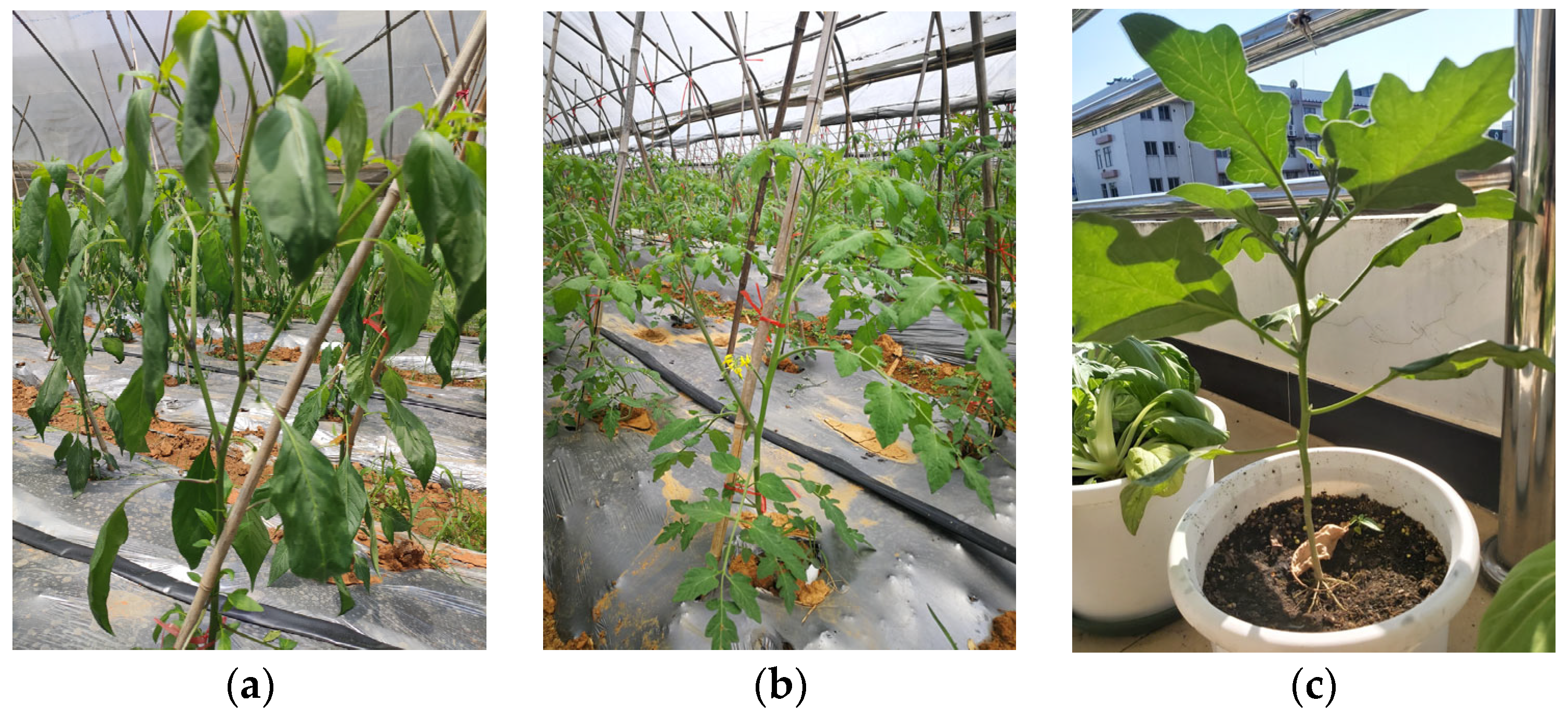
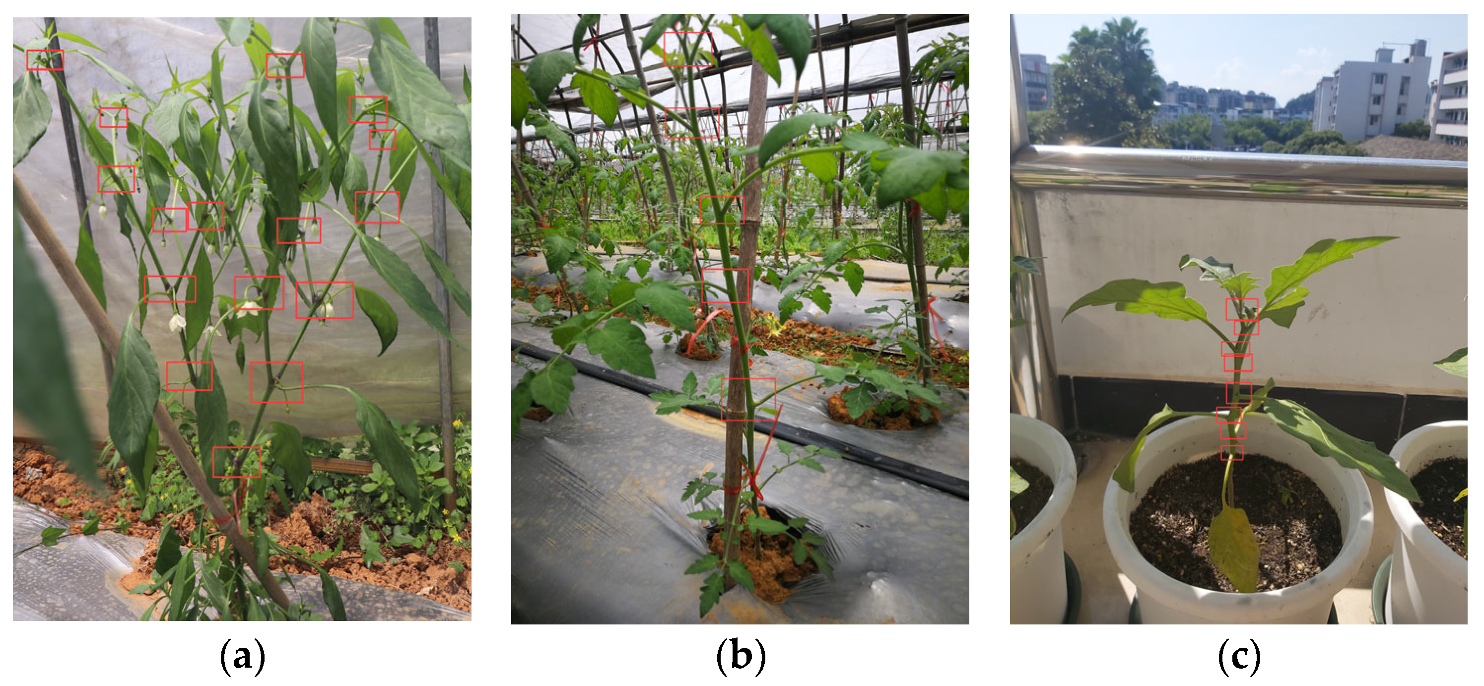
The datasets used in this study included chilies, tomatoes, and eggplants. The chilies and tomatoes were grown in a natural environment, the eggplants were cultivated in a greenhouse environment, and all plants were in a growing state. The equipment we used to capture images was the EOS R6 Mark II camera with a resolution of 3984 × 2654, the Samsung A60 phone with a resolution of 3024 × 4032, and a Redmi K20 phone with a resolution of 2976 × 3968. Images of chilies and tomatoes were captured in May 2022, at an agricultural plantation located at Yanshan town, Guilin City, Guangxi Province. Images of eggplants were captured from 15 October to 14 November 2021 at Guilin City, Guangxi Province.

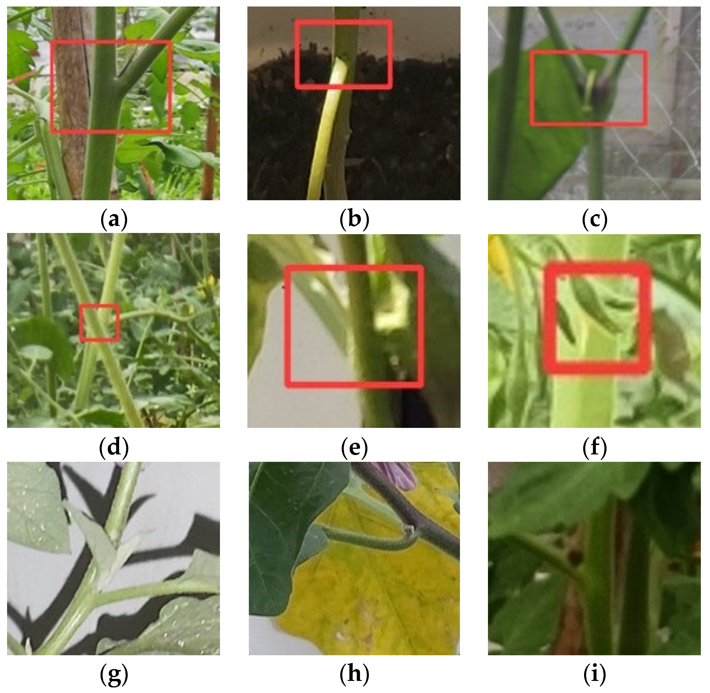
The final collected images of the chili, eggplant, and tomato plants comprised 50, 180, and 350 images, respectively. Figure 1 shows some examples. The total number of pictures of the three types of crops was 580, including 4455 nodes, with an average of 6 nodes per picture. The information for the original dataset is shown in

Table 1. Original dataset information for each crop.

Title 1	Number of Images	Total Number of Nodes	Total Number of Nodes
Chili	50	304	6
Tomato	350	2403	7
Eggplant	180	1748	10
All	580	4455	6

All: three categories of crops.

.

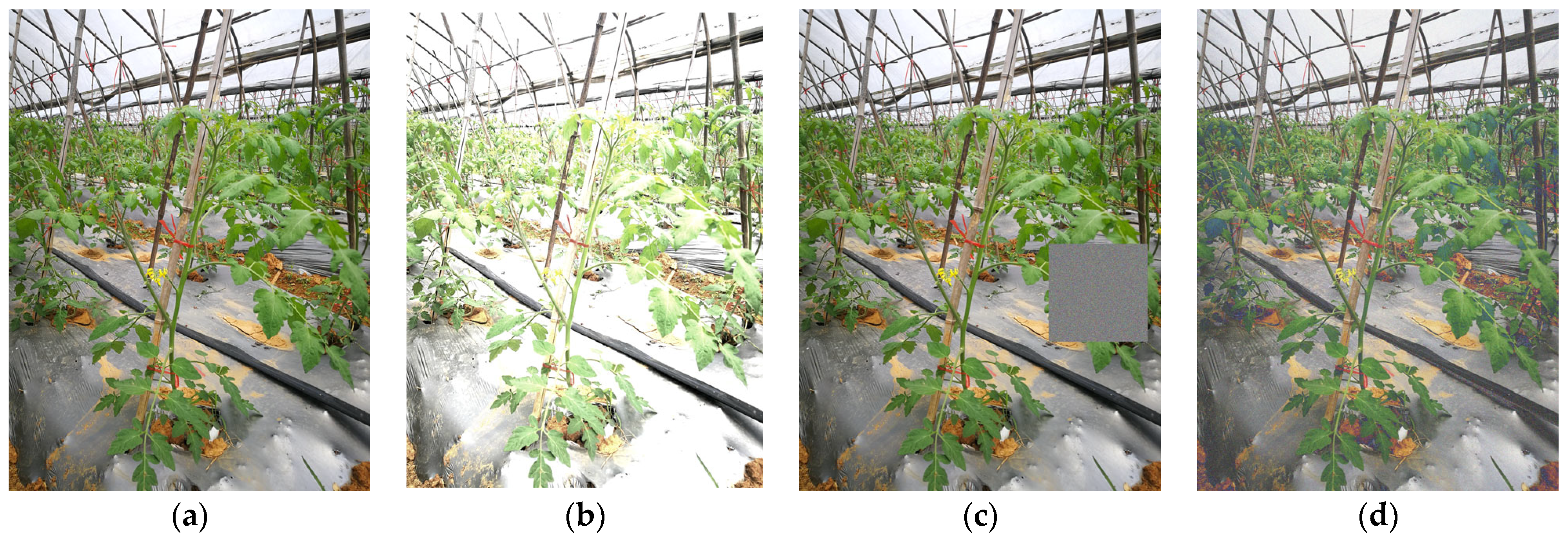
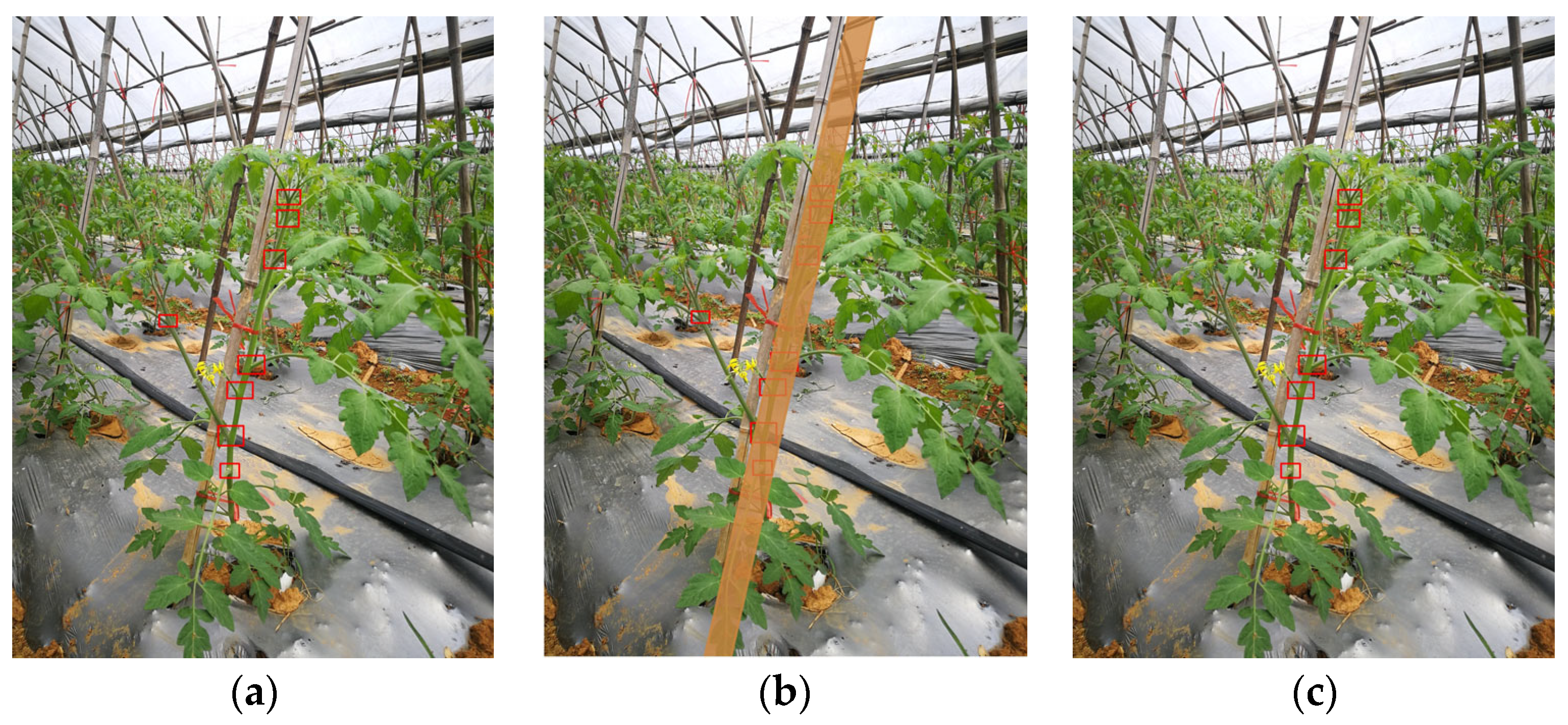
The LabelImg tool was used for labeling. In order to enhance the robustness and the average accuracy of the algorithm model, random brightness changes, random erase, and added Gaussian noise were used to augment the data. The number of images increased from 580 to 1500, while the training set and the verification set were divided according to a ratio of 8:2. Figure 2 shows some examples of different data augmentation methods.

2.2. The Overall Pipeline of the Proposed Method

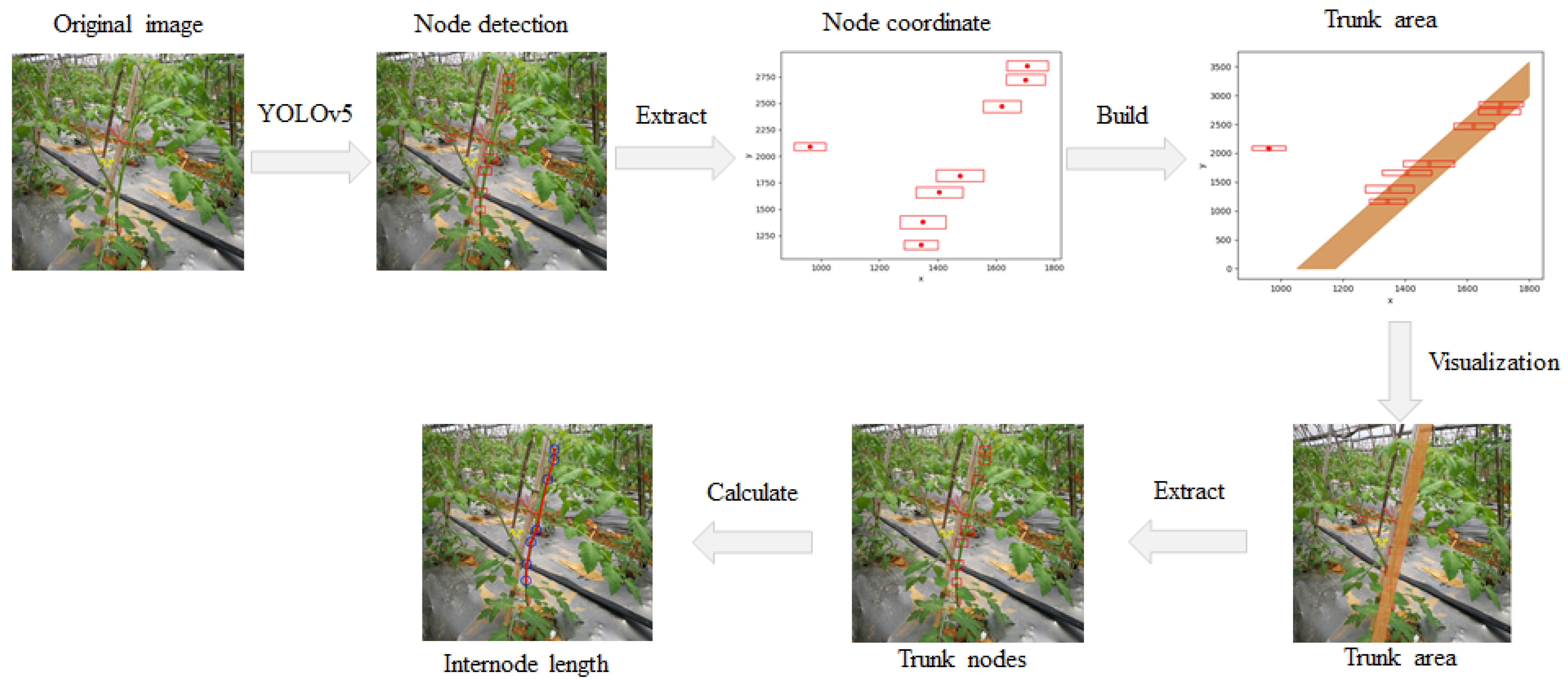
Our method was inspired by the study from Boogaard [15], and we optimized their method. Figure 3 shows the complete pipeline for our approach, which mainly includes the following three steps:

• The object detection algorithm (improved YOLOv5) is trained for node detection.
• The trunk node extraction and node order are determined.
• The internode length is estimated.

2.3. Node Detection Based on Deep Learning

The purpose of the object detection algorithm is to determine the location and category information of the object of interest in an image. The current object detection algorithm is mainly divided into two-stage detection and single-stage detection algorithms [16]. The two-stage detection algorithm first generates candidate regions, and then performs classifications and regressions on the generated candidate regions to obtain the location and category information of the object, such as the R-CNN series [17,18,19,20]. The single-stage detection algorithm directly performs regressions to obtain the detection object, such as the YOLO series [21,22,23,24,25]; SSD [26]; RetinaNet [27]; etc. Compared with the two-stage detector, the detection speed of the single-stage detector is greatly improved, while also ensuring better detection accuracy.

2.3.1. YOLOv5 Object Detection Network

The YOLOv5 detector used in this study is a relatively new version of the YOLO series algorithms, which include the early versions: YOLOv1 [21], YOLOv2 [22], and YOLOv3 [23]. YOLOv3 uses Darknet53 to extract features and has a structure similar to the feature pyramid network (FPN) [28], used for multi-scale feature fusions and multi-scale predictions. Compared with YOLOv3, the YOLOv5 algorithm mainly uses CSP Darknet53 [29] as the backbone network for feature extraction and Path Aggregation Network (PANet) [30] as the neck structure; the detection head is used by the convolutional layers for classification and bounding box regression. 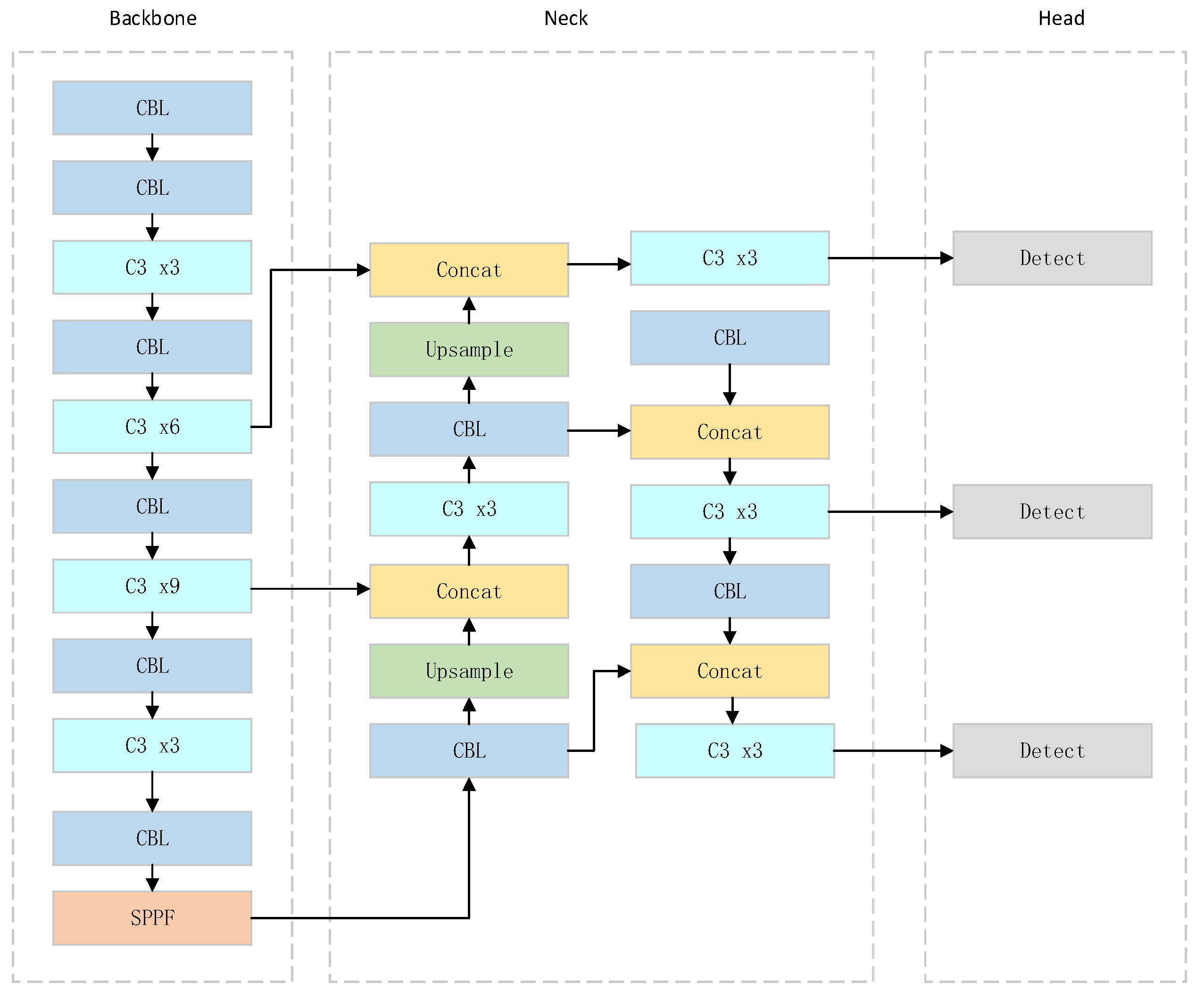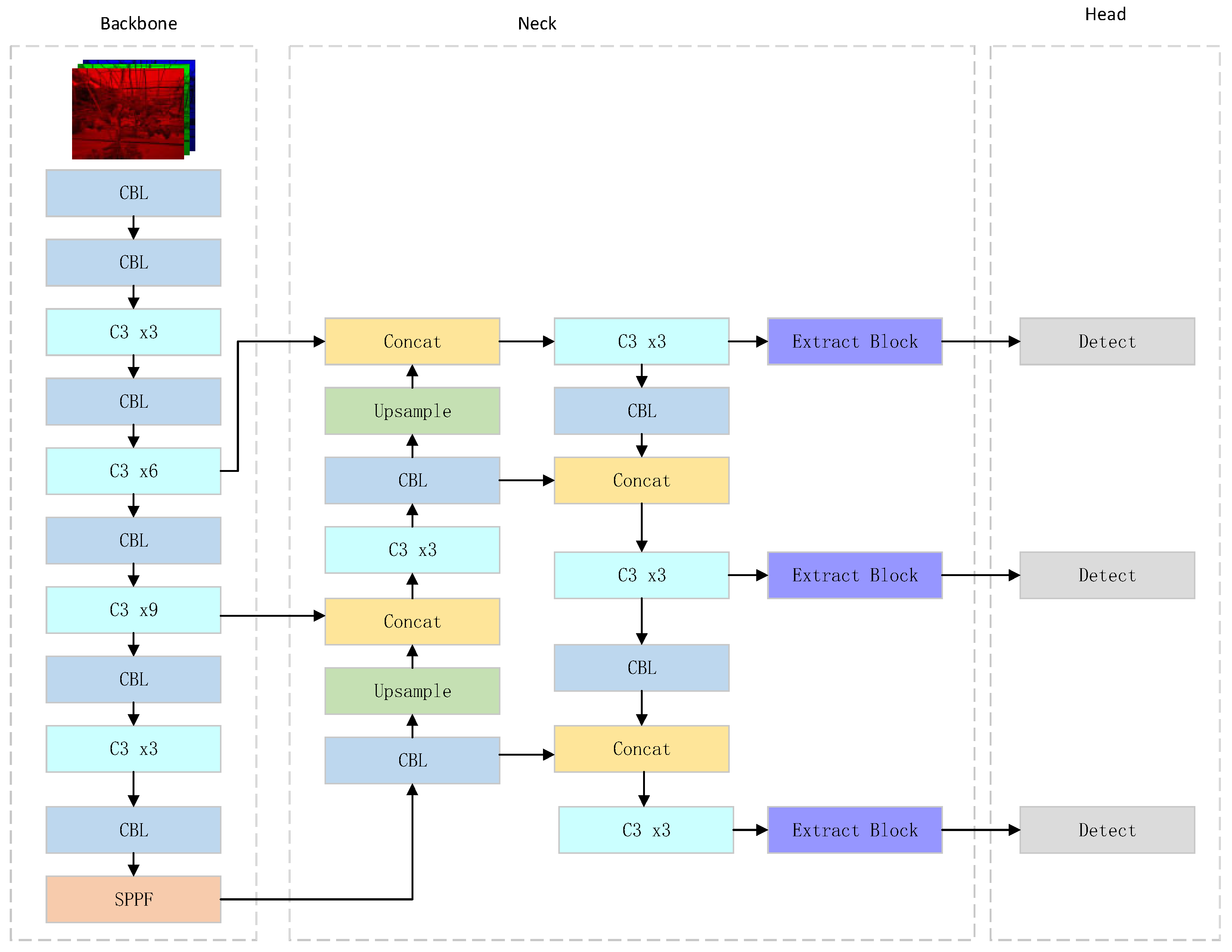Figure 4 shows the architecture of YOLOv5.

As Figure 4 shows, the YOLOv5 architecture consists of three parts: the backbone network, a neck, and a detection head. Initially, the backbone performs the CBL layer twice, then, stacks the CBL layer and C3 module continuously, before finally passing through an SPPF module. The backbone performs feature extraction on the input image and finally generates three feature maps. The input image is resized to 640 × 640, and the final output sizes are 80 × 80, 40 × 40, and 20 × 20. The neck chooses the PANet structure, and PANet adds bottom-up feature extraction on the basis of the FPN and finally merges so that the multi-scale features can be better fused. The function of the neck network is to fuse the feature maps of the three different scales generated from the backbone network, to reduce the information loss during the feature extraction process, add more context information, and output new feature maps of the three scales to obtain a better detection capability. The detection head consists of three convolutional layers that output the corresponding vectors of the feature maps of the three scales, and each vector represents the bounding box and category information of the target in the input image.

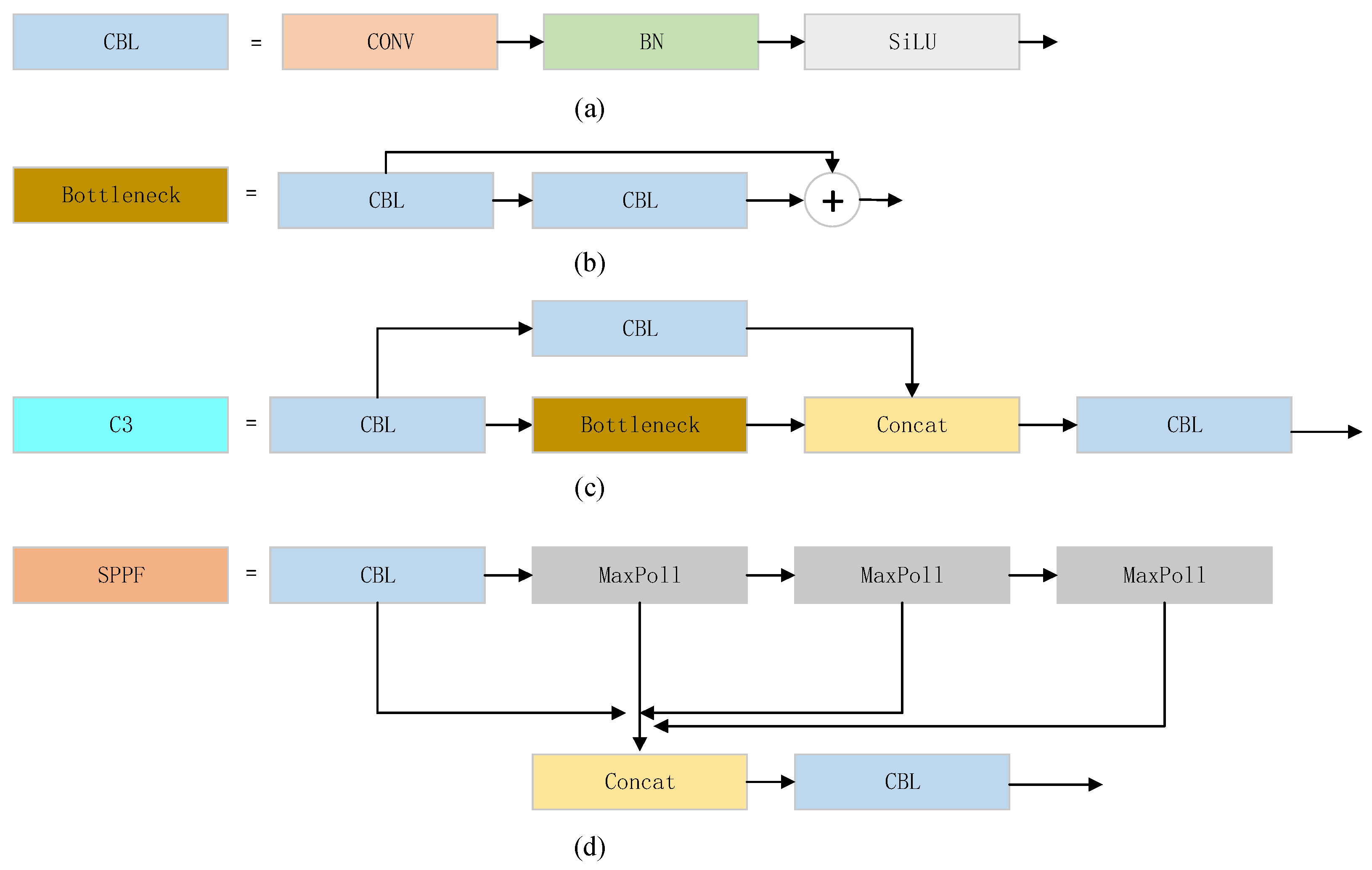
The CBL module consists of convolution, batch normalization, and a SiLU activation function, see Figure 5a. The C3 module is the key component of the network. The input of the C3 module is divided into two branches, both of which perform convolution operations, allowing the CBL module to halve the number of channels of the feature map. Then, the output feature maps of the second branch pass through the bottleneck module and the CBL layer and are residually connected by the Concat operation. Finally, through the CBL layer again, the output feature map of the module is generated, as shown in Figure 5b,c. The C3 module has a residual structure similar to ResNet [31], which is mainly used to go deeper into the network while reducing over-fitting and enhancing the function of feature extraction. SPPF is located at the last layer of the backbone, as shown in Figure 5d. SPPF uses the CBL layer to change the feature dimension, then, passes through three max-pooling layers, connects the output feature maps of the three max-pooling layers through the Concat operation, and finally obtains the output feature map through a CBL layer.

2.3.2. Improvements to the YOLOv5

This study proposes to improve the YOLOv5. A feature map extraction module is used before the detection head to enhance the feature extraction learning capabilities of the network and improve the detection accuracy of the original network. The SIoU loss [32] is used to replace the loss function of the original network to better represent the object bounding box loss, improve the detection accuracy, and increase the convergence speed of the network. The improved YOLOv5 model architecture is shown in Figure 6.

Figure 7 shows the feature extraction module with a residual structure consisting of 1 × 1 convolution, 3 × 3 convolution, and an SE (squeeze-and-excitation) [33] attention mechanism. The 1 × 1 convolution reduces the feature map dimension, reducing the parameters and calculation of the overall module; then, a 3 × 3 convolution is used for feature extraction. The residual connection is used to fuse the input features with the features after the convolution operation, guaranteeing the reuse of feature information. It finally connects to a SE attention mechanism, and the core of the SE attention mechanism is a squeeze module and an excitation module, which are used to collect global information, capture channel relationships, and improve representation capabilities.

The SE attention mechanism consists of two parts: The squeeze module and the excitation module, as shown in Figure 8. The extrusion module collects the global spatial information of the feature through the global average pooling operation; the excitation module is used to capture the channel relationship and output the feature vector by using the fully connected layer, and the ReLU and sigmoid activation functions. Then, each channel of the input feature is scaled by multiplying the feature vector with the input feature. The SE attention plays the role of emphasizing important information channels while suppressing noise, and it requires low computing resources. It can be directly added behind any module without producing a large burden of computing resources on the network.

The original YOLOv5 uses the CIOU loss [29] as the bounding box loss function, which considers the distance between the ground truth box and the predicted box, the shape, and the loss of IoU. However, this bounding box loss function does not consider the direction loss between the ground truth box and the predicted box. This study used the original bounding box loss function replaced by the SIoU loss. Compared with the CIOU loss, the direction loss is introduced, which represents the loss between the ground truth box and the predicted box more reasonably.

SioU loss consists of four costs: angle, distance, shape, and IoU. The angle cosy represents the angle difference between the ground truth box and the predicted box as a variable. Its definition is shown in Equation (2).

$$x=\frac{max\left(b_{c_y}^{gt},b_{c_y}\right)-min\left(b_{c_y}^{gt},b_{c_y}\right)}{\sqrt{{\left(b_{c_x}^{gt}-b_{c_x}\right)}^2+{\left(b_{c_y}^{gt}-b_{c_y}\right)}^2}}$$

(1)

$$\Lambda =1-2\times {\sin }^2\left(\arcsin \left(x\right)-\frac{\pi }{4}\right)$$

(2)

In Equation (2), $\left(b_{c_x}^{gt},b_{c_y}^{gt}\right)$ and $\left(b_{c_x},b_{c_y}\right)$ represent the coordinates of the center point of the ground truth box and the predicted box. Taking the angle loss as a variable of the distance loss better calculates the loss caused by the angle. The definition of distance cost is shown in Equation (3).

$$\Delta ={\displaystyle \sum }_{t=x,y}\left(1-{\mathrm{e}}^{-\gamma {\rho }_t}\right)$$

(3)

Both ${\rho }_x$ and ${\rho }_y$ measure the distance between the ground truth box and the predicted box and their definitions are shown in Equations (4) and (5). Further, Λ represents the angle cost, which integrates the angle cost into the distance loss as a variable and can express the loss more accurately.

$${\rho }_x={\left(\frac{b_{c_x}^{gt}-b_{c_x}}{c_w}\right)}^2$$

(4)

$${\rho }_y={\left(\frac{b_{c_y}^{gt}-b_{c_y}}{c_h}\right)}^2$$

(5)

$$\gamma =2-\Lambda$$

(6)

The definition of the SIoU loss is shown in Equation (7).

$$L_{box}=1-IoU+\frac{\Delta +\Omega }{2}$$

(7)

For Equation (7), $\Delta$ represents the modified distance cost, while $\Omega$ and $IoU$ represent shape cost and distance cost.

2.4. Trunk Node Extraction and Determining the Node Order

This study calculated the length between the continuous nodes on the trunk. For the chili, tomato, and eggplant plants in a growth state, most of the detected nodes are nodes on the trunk. However, some nodes of other branches were detected by the current model. We proposed a method to filter these nodes and extract the trunk nodes. The specific steps are shown in Algorithm 1.

Algorithm 1. Trunk node extraction

Input: List of bounding boxes coordinates,

Output: List of trunk node bounding boxes coordinates

Initialize trunks = []

Initialize top_point = buttom_point = (0, 0)

Get top_box, buttom_box, max_length from boxes

if top_box(x2) >= buttom_box(x2):

top_point = top_box(x2, y2)

buttom_point = buttom_box(x2, y2)

else:

top_point = top_box(x1, y2)

buttom_point = buttom_box(x1, y2)

end if

Calculate the equation of a line by top_point and buttom_point

Calculate translation line by line and max_length

Construct trunk area between two lines

for each box ∈ boxes do

if box intersect with area:

add box to trunks

end if

end for

return trunks

The results in Figure 9 show that Algorithm 1 can filter out the false detection node information that is not related to the trunk node.

To calculate the internode length, we needed to determine the order of the nodes to find the adjacent nodes. We directly sorted the trunk nodes according to their vertical coordinates from the top to the bottom in the final order. We treated the adjacent numbers as adjacent nodes, and the distance between the adjacent nodes was calculated.

2.5. Internode Length Estimation

After determining the order of the nodes, the distance between the distance nodes in the image was determined. The nodes were labeled in the determined order, the bounding box coordinates of two adjacent nodes were selected to calculate the center point coordinates, and then the pixel distance between the two nodes was calculated based on the two center point coordinates. The estimated internode length ${\widehat{S}}_{ij}$ was calculated with $i$ and node $j$. The Euclidean distance between the center coordinates of node $i$ and node $j$ on the image was calculated. ${\widehat{S}}_{ij}$ is shown in Equation (8).

$${\widehat{S}}_{ij}=\sqrt{{\left(x_i-x_j\right)}^2-{\left(y_i-y_j\right)}^2}$$

(8)

2.6. Evaluation Metrics

In this experiment, average precision (AP) and F₁ score were used as indicators to evaluate the performance of the object detection algorithms. The average precision (AP) is an important indicator to measure the accuracy of the network. When the intersection over union (IoU) of the predicted frame and the real marked frame is greater than the set threshold, the predicted frame is marked as a positive sample; otherwise, it is marked as a negative sample. True positive (TP) represents the number of positive samples that are correctly classified, and false positive (FP) represents the number of positive samples that are incorrectly classified. True negative (TN) is the number of negative samples that are correctly classified, and false negative (FN) is the number of negative samples that are incorrectly classified. The calculations of precision (P) and recall (R) are shown in Equations (9) and (10).

$$P=\frac{TP}{TP+FP}$$

(9)

$$R=\frac{TP}{TP+FN}$$

(10)

The F₁ score is another measure of precision (P) and recall (R), as shown in Equation (11).

$$F_1=\frac{2\times P\times R}{P+R}$$

(11)

The average precision (AP) is calculated by using Equation (12).

$$AP={{\displaystyle \int }}_0^{1}P\left(R\right)dR$$

(12)

The node order accuracy is calculated with Equation (13), it is the result of dividing the number of correctly numbered node predictions $N{P}_c$ and $NP$. $NP$ is the total trunk node of the prediction nodes.

$$A=\frac{N{P}_c}{NP}\times 100\%$$

(13)

The performance of the complete pipeline was evaluated by the error ($E_{ij}$) between the estimated internode length (${\widehat{S}}_{ij}$) and the ground truth internode length ($S_{ij}$), as in Equation (14).

$$E_{ij}={\widehat{S}}_{ij}-S_{ij}$$

(14)

We also calculated the relative error, as shown in Equation (15).

$$R={\displaystyle \sum }_{n=1}^N\frac{{\widehat{S}}_{ij}-S_{ij}}{S_{ij}}\times 100\%$$

(15)

In Equation (14), ${\widehat{S}}_{ij}$ and $S_{ij}$ represent the estimated length and the real length between each adjacent node, and $N$ represents the number of images.

2.7. Training the Node Detection Model

Thus, the above improved YOLOv5 was implemented and trained using the images mentioned in Section 2.1. The computer configurations used for training were as follows: the Intel Xeon Gold 6230 CPU, NVIDIA Tesla V100 GPU, and the Ubuntu 18.04 operating system. The YOLOv5 model was implemented by using the PyTorch framework with Python as the programing language. Some required libraries including CUDA, cuDNN, and OpenCV were also used.

In this study, the YOLOv5 was trained in an end-to-end manner using stochastic gradient descent (SGD). The resolution of the input image was resized to 640 × 640, the batch size was set to 32, and the training epoch was set to 100.

Table 2. The hyperparameter settings for the network training.

Hyperparameter	Value
Optimization	SGD
Initial learn rate	0.01
Momentum	0.937
Weight decay	$5\times {10}^{-4}$
Mini-batch size	32
Number of epochs	100

shows the specific settings of the network training hyperparameters. The weight file of the trained detection model was used to evaluate the performance of the model by using the verification set.

3. Results

Several experiments were conducted and tested to evaluate the performance and availability of our proposed method for crop node detection and internode length estimation based on the improved YOLOv5, using the evaluation metrics described in Section 2.6.

3.1. Node Detection

Table 3. Comparison of the results among several object detection networks.

Methods	Parameters	GFLOPs	Average Time (ms)	Precision (%)	Recall (%)	F1 Score (%)	AP (%)
YOLOv7	37.2M	103.2	7.68	92.1	85.2	88.5	90.4
YOLOv7-tiny	6.0M	13.0	3.3	87.7	72.1	79.1	81.8
YOLOv5s	7.0M	15.8	2.6	92	83	87.3	89.1
Ours	9.4M	23.1	2.96	93.1	85.1	88.9	90.5

GFLOPS: Giga floating-point operations per second.

provides details of the experimental results. The accuracy, recall, F1 score, and average precision on the validation set after training were 93.1%, 85.1%, 88.9%, and 90.5%, respectively. Compared with the original YOLOv5s, the F1 score increased by 1.6%, and the average precision increased by 1.4%, indicating that the detection ability of our proposed YOLOv5 model has been improved with an increase in parameters only by 2.4 M. After improvement, the detection time was 2.96 ms per image, thereby achieving higher performance with less computational overhead. We compared it with YOLOv7 and YOLOv7-tiny, and our improved YOLOv5 models achieved the best detection performance.

In order to observe the detection performance of the algorithm more deeply, some typical examples are shown in Figure 10 and Figure 11. Figure 10 shows our detection method results in three types of crops: chili, tomato, and eggplant. Figure 11 shows examples of the detected nodes. The first row of the image shows three correctly identified nodes. Although the appearance of the three nodes changed greatly, the network could still detect them. The second row shows some examples of false positives. Figure 11d shows that the intersection of the two branches was detected as a node. This was due to the visual difference, and this part produced image features that were similar to the node. In Figure 11 e and f, intersections were detected as nodes due to their partial occlusion by the leaves, flowers, and branches. Figure 11g–i shows three false negative examples, where these nodes were ground truth labeled data, yet were not detected by the algorithm. Thus, demonstrating that it is still difficult for node detection algorithms to detect nodes in complex backgrounds.

3.2. Determining the Node Order

We selected 10 images from each crop in the validation set, and a total of 30 images were used to determine the node order. The node order is based on the comparison between the detected trunk nodes and the ground truth trunk nodes, while the same number of nodes indicates that the node order is correct.

Table 4. Determination of the accuracy of the node order.

Crops	Methods	Ground Truth		Detect		Accuracy Number	Rate (%)
		All Node	Trunk Node	All Node	Trunk Node
Chili	YOLOv5s	62	32	62	32	32	100
	Ours	62	32	62	32	32	100
Eggplant	YOLOv5s	91	68	90	67	58	86.6
	Ours	91	68	90	69	64	92.8
Tomato	YOLOv5s	57	43	59	44	32	72.7
	Ours	57	43	61	44	42	95.5
All	YOLOv5s	210	143	211	143	122	85.3
	Ours	210	143	213	145	138	95.2

shows the results of the detected node order. Most of our methods determined the correct node order, and the accuracy rate of the node order reached 95.2%. Compared with the original YOLOv5s model, this result proved that our improved algorithm had a better detection performance.

3.3. Internode Length Estimation

The estimation of the internode length was also conducted from the above 30 images. The internode length calculated from the distance between adjacent nodes, with the label node bounding box, was used as the ground truth value. The estimated internode length calculated from the detected nodes was then compared to its ground truth.

Table 5. The Compared results on internode length estimation.

Methods	Average Error (Pixels)	Relative Error (%)
YOLOv7	33.95	7.27
YOLOv7-tiny	143.20	21.9
YOLOv5s	47.14	8.97%
Ours	41.30	7.36%

shows that YOLOv7 achieved the best estimation accuracy, while our improved YOLOv5 achieved an estimation accuracy similar to YOLOv7, however, it was faster and consumed fewer computing resources.

Table 6. Comparison of the results in the three categories of crops.

Crops	Methods	Average Error (Pixels)	Relative Error (%)
Chili	YOLOv5s	12.374	2.64%
	Ours	10.59	1.58%
Eggplant	YOLOv5s	89.16	17.86%
	Ours	66.26	13.16%
Tomato	YOLOv5s	37.43	5.40%
	Ours	50.44	7.96%
All	YOLOv5s	47.14	8.97%
	Ours	41.30	7.36%

shows the results of the method in different crops. The estimated internode length calculated by using our improved YOLOv5 achieved better performances in chili and eggplant.

4. Discussions

This study proposed a method to calculate the internode lengths. The method included a node detection algorithm, a combined trunk node extraction algorithm, and an internode length estimation.

Our improved YOLOv5 adds a feature extraction module and replaces the loss function, we have designed an ablation experiment at the node detection step and a complete pipeline. The performance of our improvement is verified by ablation experiments, and the results of the ablation experiments are shown in

Table 7. Result of ablation experiments in the node detection step.

	Precision (%)	Recall (%)	F1 Score (%)	AP (%)
Baseline	0.92	0.83	0.87303	0.891
+Extraction block	0.916	0.85	0.8822	0.904
+SIoU loss	0.931	0.851	0.88905	0.905

and

Table 8. Result of ablation experiments in the complete pipeline.

	Average Error (Pixels)	Relative Error (%)
Baseline	47.14	8.97%
+Extraction block	59.73	11.0%
+SIoU loss	41.30	7.36%

. In the node detection step, with the feature extraction module, the recall rate increased by 2%, although the accuracy decreased by 0.4%, whereas the F1 score and average precision increased by 0.9% and 1.3%, respectively. After replacing the SIoU loss, the accuracy increased by 1.1%, the recall rate increased by 2.1%, while the F1 score and the average precision increased by 1.6% and 1.4%, respectively. In the complete pipeline, when we added the feature extraction module, the average error, and relative error increased by 12.59 pixels and 2.03%, respectively, although with the SIoU loss, the average error and the relative error decreased by 5.84 pixels and 1.61%, respectively. These results indicate that our improved network can improve the performance of the network.

However, we discovered some false positive results. We assumed that the overlap of the crop organs in the natural background from a single perspective was serious. The overlapping of different branches, leaves, flowers, and branches all resulted in quite similar node characteristics, which caused the network to detect these features as nodes, leading to false positives. The current method is suitable for crop plants that grow vertically in the growth stage because the plants in this period grow upwards with fewer branches, and the leaves are not too lush, thus, the occlusion is not serious, and the nodes can generally be detected successfully.

The internode length of the trunk node is the expected calculation goal. However, the node order is hard to decide because the nodes on subbranches would also be detected Previously, Yamamoto et al. [13] estimated the internode length of tomato seedlings, and Boogaard et al. [15] measured the internode length of cucumber plants in the growth state. These plants have no branches other than the trunk. Crops such as chili and eggplant have many branches, so we designed steps to extract the trunk nodes. Yamamoto et al. [13] and Boogaard et al. [15] clustered the node coordinates using affinity propagation for determining the node order. They first obtained node clusters in different orders according to the clustering and then sorted the node according to the vertical coordinates. We used affinity propagation to obtain node clusters, although this did not obtain good results, and instead increased the complexity of the algorithm. We assumed they used the same batch of crop images taken at different time periods for detection, and the positions and numbers of nodes were not much different. The positions of the crop nodes on the images in our experiment were quite different, and the number of nodes was inconsistent, indicating that clustering using node coordinates does not achieve good results. Directly determining the node order according to the node vertical coordinates can obtain better results. Our method decides the adjacent nodes according to the vertical coordinates of a node. Assuming that the trunk is horizontal or rotated, our method is not applicable. Presently, our method is limited to vertically growing plants and growing agricultural crops because the crop branches are obvious and vertical.

Our complete pipeline had an average error of 41.3 pixels and a relative error of 7.36%. In Figure 12, we compare the estimated internode length with the ground truth internode length; the red line is the ground truth length, and the blue scatter point is our estimated length, and we also calculated the root mean square error (RMSE) of the model as 2.16 and the R-squared error as 0.997.

5. Conclusions

In this study, we proposed an improved YOLOv5-based node detection and internode length estimation method. The results indicate that the network showed improvements in node detection performance. Generally speaking, plants have many branches, and the nodes of different branches will also be detected, yet adjacent nodes cannot be determined. We extracted the trunk nodes to estimate the internode length. Our method is suitable for plants that grow vertically, most of which have not yet grown many branches. In the future, we will realize the conversion of the estimated pixel distance between nodes into the actual length and deploy it on the embedded platform, to record the length data of plants between nodes at regular intervals.